x

Commentaries from the edited collection of reprints

Gauge Theories of Gravitation

A Reader with Commentaries

Imperial College Press, London, April 2013

https://doi.org/10.1142/p781

Editors :

Milutin Blagojević

Institute of Physics, University of Belgrade

Friedrich W. Hehl

Institute of Theoretical Physics, University of Cologne, and

Department of Physics and Astronomy, University of Missouri, Columbia

Foreword  by T. W. B. Kibble, FRS

Abstract

During the last five decades, gravity, as one of the fundamental forces of nature, has been formulated as a gauge theory of the Weyl-Cartan-Yang-Mills type. The present text offers commentaries on the articles from the most prominent proponents of the theory, which are a substantial part of the above reprint volume.

In the early 1960s, the gauge idea was successfully applied to the Poincaré group of spacetime symmetries and to the related conserved energy-momentum and angular momentum currents. The resulting theory, the Poincaré gauge theory, encompasses Einstein’s general relativity as well as the teleparallel theory of gravity as subcases. The spacetime structure is enriched by Cartan’s torsion, and the new theory can accommodate fermionic matter and its spin in a perfectly natural way. This guided tour starts from special relativity and leads, in its first part, to general relativity and its gauge type extensions à la Weyl and Cartan. Subsequent stopping points are the theories of Yang-Mills and Utiyama and, as a particular vantage point, the theory of Sciama and Kibble. Later, the Poincaré gauge theory and its generalizations are explored and special topics, such as its Hamiltonian formulation and exact solutions, are studied. This guide to the literature on classical gauge theories of gravity is intended to be a stimulating introduction to the subject.

Classification of Gauge Theories of Gravity

The acronyms and symbols in the figure have the following meanings:

PG = Poincaré gauge theory (of gravity)

EC = Einstein–Cartan(–Sciama–Kibble) theory (of gravity)

GR = general relativity (Einstein’s theory of gravity)

TG = translation gauge theory (of gravity) also known as teleparallel theory (of gravity)

GR_|| = a specific TG known as teleparallel equivalent of GR (“GR teleparallel")

WG = Weyl(–Cartan) gauge theory (of gravity)

MAG = metric-affine gauge theory (of gravity)

CG = conformal gauge theory (of gravity),

AdSG = (anti-)de Sitter gauge theory (of gravity)

SuGra = supergravity (super-Poincaré gauge theory of gravity)

rectangle ${\square}\rightarrow$ class of theories, circle ${\bigcirc}\rightarrow$ definite viable theories

nonmetricity $Q=Q\diagup+\frac{1}{4}({\rm tr}\hskip 1.00006ptQ)1$, torsion $T$, curvature $R$.

Contents

Doc-Start chapter*.1 chapter*.2 chapter*.3 chapter*.4 chapter*.5 chapter*.6 part.1 chapter.1 chapter.2 chapter.3 part.2 chapter.4 chapter.5 chapter.6 chapter.7 part.3 chapter.8 chapter.9 chapter.10 chapter.11 chapter.12 part.4 chapter.13 chapter.14 chapter.15 chapter.16 chapter.17 chapter.18 chapter.19 chapter*.7

Foreword

Symmetry has always played a big role in physics. Advancing understanding has time and again revealed previously unknown symmetries. Isaac Newton abandoned the idea of a preferred origin of space, revealing the underlying translational symmetry; Albert Einstein uncovered an unexpected symmetry between time and space.

A key innovation of the twentieth century was Hermann Weyl’s invention of gauge theory, in which a global physical symmetry is replaced by a local one; the arbitrary phase in the quantum wave-function becomes a function of space and time, a change that requires the existence of the electromagnetic field. This proved to be an astonishingly fruitful idea. Today, all the components of the “standard model” of particle physics that so accurately describes our observations are gauge theories. Weyl’s “gauge principle”, that global symmetries should be promoted to local ones, applied to the standard-model symmetry group $SU(3)\times SU(2)\times U(1)$, is enough to yield the strong, weak and electromagnetic interactions.

Only gravity is missing from this model. But it too shows many of the same features. Going from special to general relativity involves replacing the rigid symmetries of the Poincaré group—translations and Lorentz transformations—by freer, spacetime dependent symmetries. So it was natural to ask whether gravity too could not be described as a gauge theory. Is it possible that starting from a theory with rigid symmetries and applying the gauge principle, we can recover the gravitational field? The answer turned out to be yes, though in a subtly different way and with an intriguing twist. Starting from special relativity and applying the gauge principle to its Poincaré-group symmetries leads most directly not precisely to Einstein’s general relativity, but to a variant, originally proposed by Élie Cartan, which instead of a pure Riemannian spacetime uses a spacetime with torsion. In general relativity, curvature is sourced by energy and momentum. In the Poincaré gauge theory, in its basic version, there is also torsion, sourced by spin.

As someone who was involved in the early stages of this development, I am astonished and intrigued by how the theory has developed over the last half century. Reading this book makes it clear how wide its ramifications have spread. Over the years, Poincaré gauge theory has been put on a much firmer mathematical base. In its simplest form, it gives predictions that are in almost all observational situations identical with those of general relativity, but in situations of extremely high density there are significant differences. These differences may be of profound importance for the physics of the very early universe and of black holes, and could one day be subject to observational test.

Moreover, Poincaré gauge theory is not necessarily the end of the story. There are several possible extensions, in which the basic symmetry group is even larger; the Poincaré group may be augmented by the inclusion of dilatations or even enlarged to the full group of affine transformations. The resulting theories, the Weyl–Cartan theory and the metric-affine gravity theory, have some very attractive features. Only time will tell whether any of these intriguing theories is correct and which of the hypothesized hidden symmetries is actually realized in nature. For anyone interested is pursuing these ideas, this book certainly provides a fascinating and very valuable resource.

London, March 2012 Professor Tom Kibble, FRS

Imperial College London

Preface

We have been both fascinated by gauge theories of gravity since the 1960s and the 1970s and have followed the subject closely through our own work. In this reprint volume with commentaries we would like to pass over our experience to the next generation of physicists. We have tried to collect the established results and thus hope to prevent double work and to focus new investigations on the real loopholes of the theory.

The aim of this reprint volume with commentaries is to introduce graduate students of theoretical physics, mathematical physics or applied mathematics, or any other interested researcher, to the field of classical gauge theories of gravity. We assume that our readers are familiar with the basic aspects of classical mechanics, classical electrodynamics, special relativity (SR), and possibly elements of general relativity (GR). Some knowledge of particle physics, group theory, and differential geometry would be helpful.

Why gauge theory of gravity? Because all the other fundamental interactions (electroweak and strong) are described successfully by gauge theories (of internal symmetries), whereas the established gravitational theory, Einstein’s GR, seems to be outside this general framework, even though, historically, the roots of gauge theory grew out of a careful analysis of GR. A full clarification of the gauge dynamics of gravity might be the last missing link to the hidden structure of a consistent unification of all the fundamental interactions at both the classical and the quantum level.

Our book is intended not just to be a simple reprint volume, but more a guide to the literature on gauge theories of gravity. The reader is expected first to study our introductory commentaries and become familiar with the basic ideas, then to read specific reprints, and after that to return again to our text, explore the additional literature, etc. The interaction is expected to be more complex than just starting with commentaries and ending with reprints. A student, guided by our commentaries, can get self-study insight into gauge theories of gravity within a relatively short period of time.

The underlying structure of gravitational gauge theory is the group of motions of the spacetime in SR, namely the Poincaré group $P(1,3)$. If one applies the gauge-theoretical ideas to $P(1,3)$, one arrives at the Poincaré gauge theory of gravity (PG). Therein, the conserved energy-momentum current of matter and the spin part of the conserved angular momentum current of matter both act as sources of gravity. The simplest PG is the Einstein–Cartan theory, a viable theory of gravity that, like GR, describes all classical experiments successfully. On the other hand, if one restricts attention to the translation subgroup of $P(1,3)$, one ends up with the class of translation gauge theories of gravity, one of which, for spinless matter, can be shown to be equivalent to GR. The developments that led to PG are presented in Part A of our book; in Part B, definite and enduring results of PG are displayed. The content of Parts A and B should be considered as a mandatory piece of the general education for all gravitational physicists, while the remaining two parts cover subjects of a more specialized nature.

Since SR is such a well-established theory, from a theoretical as well as from an experimental point of view, the gauging of $P(1,3)$ rests on a very solid basis. Nevertheless, there arise arguments as to why an extension of PG seems desirable; they are presented in Part C. As a finger exercise, we gauge the group of Poincaré plus scale transformations. Then, we extend $P(1,3)$ to the general real linear group $GL(4,R)$, thus arriving at metric-affine gauge theory of gravity (MAG). This general framework leads to a full understanding of the role of a non-vanishing gradient of the metric (nonmetricity). Several other extensions treated in Part C appear to be rather straightforward tasks.

The gauge theory of gravity, since 1961, when it first had been definitely established, has had a broad development. Therefore, in Part D we display the results on several specific aspects of the theory, like the Hamiltonian structure, equations of motion for matter, cosmological models, exact solutions, three-dimensional gravity with torsion, etc. These subjects could be starting points for research projects for our prospective readers.

Clearly, making a good choice of reprints is a very demanding task, particularly if we want to take care of the historical justice and authenticity. But we also wanted to take care of another aspect—that our collection of reprints should be a useful guide to research-oriented readers without too many historical detours. These two aspects are not always compatible, and we tried to ensure a reasonable balance between them. To what extent these attempts were successful is to be judged by our readers.

$\bullet$ Chapters of the book that can be skipped at a first reading are marked by the star symbol ^∗.

October 2012

Milutin Blagojević (Belgrade)

Friedrich W. Hehl (Cologne and Columbia, Missouri)

mb@ipb.ac.rs, hehl@thp.uni-koeln.de

List of Useful Books

Here is a chronologically ordered list of books, in which readers can find useful information on the subject of gauge theories of gravity. The selection is made by requiring at least some mentioning of the EC theory.

• V. N. Ponomariev, A. O. Barvinsky, and Yu. N. Obukhov,
  Geometrodynamical Methods and the Gauge Approach to the Theory of Gravitational Interactions (Energoatomizdat, Moscow, 1985) (in Russian). Revised edition:
  Gauge Approach and Quantization Methods in Gravity Theory (Nauka, Moscow, 2017) (in English). This edition offers a list of 3136 references on gauge theories of gravity.

• W. Thirring, A Course in Mathematical Physics 2: Classical Field Theory, 2nd ed., translated by E. M. Harrell (Springer, New York, 1986).

• E. W. Mielke, Geometrodynamics of Gauge Fields—On the Geometry of Yang–Mills and Gravitational Gauge Theories (Akademie-Verlag, Berlin, 1987). New edition:
  Geometrodynamics of Gauge Fields, 2nd. ed. (Springer, Switzerland, 2017).

• M. Göckeler and T. Schücker, Differential Geometry, Gauge Theories and Gravity (Cambridge University Press, Cambridge, 1987).

• P. Ramond, Field Theory: A Modern Primer, 2nd ed. (Addison–Wesley, Redmond City, CA, 1989).

• W. Kopczyński and A. Trautman, Spacetime and Gravitation (PWN, Warsaw; Wiley, Chichester, 1992).

• M.  Blagojević, Gravitation and Gauge Symmetries (IoP, Bristol, 2002).

• T. Ortín, Gravity and Strings (Cambridge University Press, Cambridge, 2004).

• L. Ryder, Introduction to General Relativity (Cambridge University Press, Cambridge, 2009).

x

Part A     The Rise of Gauge Theory of Gravity
up to 1961

Chapter 1     From Special to General Relativity Theory

Reprinted papers:

• A. Einstein, The foundation of the general theory of relativity (in German), Annalen der Physik 354 [IV. Folge, Band 49], 769–822 (1916). Extract from p. 769 to p. 779.

1.1 Special relativity

With the advent of special relativity theory (SR) at the beginning of the twentieth century, there emerged a unified spacetime structure for classical mechanics and classical electrodynamics, namely the Minkowski space $M_{4}$. The latter is a 4-dimensional pseudo-Euclidean space with one time coordinate, $X^{0}$, and three Cartesian spatial coordinates, $X^{1},X^{2},X^{3}$, the “pseudo” referring to the fact that the 4-dimensional metric is not positive definite, the line element rather reads

$$ds^{2}=(dX^{0})^{2}-(dX^{1})^{2}-(dX^{2})^{2}-(dX^{3})^{2}=\eta_{\mu\nu}\,dX^{\mu}\otimes dX^{\nu}\,,$$ (1.1)

with $\eta_{\mu\nu}=\text{diag}(+1,-1,-1,-1)$. The unit of time is chosen such that the speed of light is $1$. The coordinates used in (1.1) are called 4-dimensional (4d) Cartesian (or Minkowski) coordinates.

The group of motions in an $M_{4}$, which, by definition, leaves the line element (1.1) invariant, is the Poincaré group (aka inhomogeneous Lorentz group), the semi-direct product of the 4d translation group $T(4)$ and the (homogeneous) Lorentz group $SO(1,3)$. Cartan called it simply the Euclidean group of the 4d Minkowski space. The Poincaré group has four generators, $P_{\mu}$, for translations and $3+3=6$ generators, $J_{\mu\nu}=-J_{\nu\mu}$, for boosts and 3d rotations, respectively, that is, altogether $4+6=10$ generators.

If the action of a physical system in an $M_{4}$ is invariant under (rigid) Poincaré transformations, then, via the first Noether theorem, the tensors of energy-momentum density, $\mathfrak{T}_{\mu}{}^{\lambda}$, and of angular momentum density, $\mathfrak{J}_{\mu\nu}{}^{\lambda}=-\mathfrak{J}_{\nu\mu}{}^{\lambda}$, of matter are divergence-free, $\partial_{\lambda}\mathfrak{T}_{\mu}{}^{\lambda}=0$ and $\partial_{\lambda}\mathfrak{J}_{\mu\nu}{}^{\lambda}=0$, and the corresponding integrated quantities, $\int d^{3}X\,\mathfrak{T}_{\mu}{}^{0}$ and $\int d^{3}X\,\mathfrak{J}_{\mu\nu}{}^{0}$, conserved. The total angular momentum density, $\mathfrak{J}_{\mu\nu}{}^{\lambda}$, can be split into an intrinsic or spin part and an orbital part, $\mathfrak{J}_{\mu\nu}{}^{\lambda}=\mathfrak{S}_{\mu\nu}{}^{\lambda}+X_{\mu}\mathfrak{T}_{\nu}{}^{\lambda}-X_{\nu}\mathfrak{T}_{\mu}{}^{\lambda}$, with the reformulated conservation law for angular momentum, $\partial_{\lambda}\mathfrak{S}_{\mu\nu}{}^{\lambda}+\mathfrak{T}_{\nu\mu}-\mathfrak{T}_{\mu\nu}=0$. The latter version of the angular-momentum conservation law—in contrast to $\partial_{\lambda}\mathfrak{J}_{\mu\nu}{}^{\lambda}=0$—is locally defined and can be straightforwardly generalized to curved and contorted spaces. These considerations on energy-momentum and angular momentum can also be applied to point particles, whereas we concentrate here on continuously distributed fields.

For point particles the Casimir operators of P(1,3), namely $P^{2}$ and $W^{2}$, with the Pauli–Lubański 4-vector $W^{\mu}:=\frac{1}{2}\epsilon^{\mu\nu\rho\sigma}J_{\nu\rho}P_{\sigma}$ (see [4]), are at the basis of the universally valid mass-spin classification of elementary particle physics (Wigner [5]). Hence the field-theoretical notions of energy-momentum density, $\mathfrak{T}_{\mu\nu}$, and spin angular momentum density, $\mathfrak{S}_{\mu\nu}{}^{\lambda}$, correspond in particle language to mass $m$ and spin $s$, respectively.

Classical mechanics had to be modified in order to fit into the Minkowski space, see [6]. The last lingering doubts about the correctness of the new special-relativistic mechanics of the year 1905 were eventually wiped out by the first nuclear explosion in Alamogordo in 1945, which demonstrated so visibly the mass-energy equivalence as predicted by SR. In contrast, classical electrodynamics, which was an established theory since 1886, when high-frequent electromagnetic waves ($\lambda\approx$ 1 m) were discovered, had only to be reinterpreted in the framework of Minkowski geometry, since it was already intrinsically special-relativistic, see [7].

1.2 Equivalence principle and gravitation

On this harmonious spacetime picture, there fell only one shadow: In spite of several attempts, the gravitational field could not be accommodated to the Minkowski spacetime. This led Einstein [8], in 1907, to a new approach: He started from the experimentally established fact (for more recent confirmations see [9]) that the inertial mass of a particle (entering Newton’s law of motion) is equal to its gravitational mass (entering Newton’s gravitational attraction law). Thus, in a prescribed gravitational field all bodies, regardless of their masses, are equally accelerated. Accordingly, a reference frame with a conceived homogeneous gravitational field can be substituted by a uniformly accelerated reference frame. The heuristic value of this equivalence principle is that information on the behavior of accelerated matter can lead to predictions about its behavior in a gravitational field or, as Einstein [Reprint 1.1] has put it, “…we are able to ‘produce’ a gravitational field merely by changing the system of coordinates”. Let us have a closer look at Einstein’s set up.

Equipment and constructs in Einstein’s “laboratory” (see [Reprint 1.1] and [10]):
(i) A neutral point particle with mass $m$; (ii) an inertial frame $K$; (iii) an accelerated (i.e., non-inertial) frame $K^{\prime}$; (iv) a homogeneous gravitational field; and (v) light rays.

To (i): The point particle has its mass $m$ as the only attribute, it is structureless, spherically symmetric, electrically and magnetically neutral, without spin. In actual fact, in calculating the perihelion shift of a planet within the theory resulting from Einstein’s heuristic procedure, namely general relativity (GR), see below, the “point particle” could be a planet, say Jupiter for example. On the other hand, in GR a point mass does not exist; each mass has a very small, but finite Schwarzschild radius attached to it. Thus, the highly idealized nature of this concept is evident.

To (ii): In Einstein’s terminology, a frame of reference is called a “system of coordinates”. The inertial frame $K$ is spanned by the four Cartesian coordinate axes $(X^{0},X^{1},X^{2},X^{3})$ of a Minkowski spacetime, with the line element (1.1). An inertial system is a reference system in which “physics laws hold good in their simplest form”.

To (iii): The non-inertial frame $K^{\prime}$ is in uniformly accelerated translational motion with respect to $K$. It is described by four curvilinear coordinates, $x^{0},x^{1},x^{2},x^{3}$ (called by Einstein $x_{4},x_{1},x_{2},x_{3}$, respectively). Its line element, derived from (1.1) by coordinate transformation $dX^{\mu}=\frac{\partial X^{\mu}}{\partial x^{\rho}}dx^{\rho}$, reads

$$ds^{2}=g_{\mu\nu}(x^{\rho})\,dx^{\mu}\otimes dx^{\nu}\,.$$ (1.2)

Einstein referred explicitly to translational acceleration $a^{\mu}$. With such an acceleration a length parameter $\ell_{\text{tr}}:=c^{2}/a$ is connected, where $a$ is the magnitude of the 3-acceleration. For the terrestrial gravitational acceleration $g$, we have $\ell_{\text{tr}}=c^{2}/g_{\oplus}\approx 10^{16}\,{\rm m}\approx 1\,\text{light year}$, see [11]. For length dimensions, $\ell_{\text{ex}}$, of usual laboratory experiments we have $\ell_{\text{ex}}\ll\ell_{\text{tr}}$, that is, Einstein’s application of the equivalence principle, as applied to laboratories on earth, obeys this inequality.

To (iv): The concept of a homogeneous gravitational field has to be applied with care. As shown in [Reprint 1.1] and below, in Einstein’s discussion of the equivalence principle the gravitational field is represented by the (noncovariant) Christoffel symbols $\widetilde{\Gamma}_{\nu\rho}{}^{\mu}$. If, at a certain point in spacetime, their first derivatives or, synonymously, their curvature $\widetilde{R}$ can be neglected, the gravitational field can be considered to be homogeneous and the equivalence principle applied. This is restricted to laboratory sizes $d$ over which $\widetilde{\Gamma}$ does not vary significantly, namely $d\ll\widetilde{\Gamma}/\widetilde{R}$. For a critical discussion of these questions, see Schucking [12].

To (v): The light rays can be extracted from (special relativistic) vacuum electrodynamics in the geometric optics limit. Incidentally, with light rays and the paths of mass points an axiomatics of the spacetime of GR can be set up, as was pointed out by Weyl [13] and worked out explicitly by Ehlers, Pirani, and Schild (EPS) [14]. This axiomatics uses only tools of Einstein’s laboratory. The result is really a Weyl geometry (see Chapter 2) and only by an ad hoc postulate, see Audretsch et al. [15, 16], one ends up with the Riemannian space of GR.

Let us now go back to [Reprint 1.1]. By means of an epistemological discussion on two rotating bodies, Einstein arrives at the thesis that the laws of physics should be of such a nature that they are equally valid in arbitrarily moving reference frames. Einstein implements this idea with the help of the well-established law of the equality of inertial and gravitational mass. Einstein studies the motion of a force-free mass in the inertial frame $K$. It moves in a straight line with constant velocity:

$$\frac{d^{2}X^{\mu}}{ds^{2}}=0\,.$$ (1.3)

The same motion, as viewed from the accelerated frame $K^{\prime}$, can be derived by a transformation of (1.3) to curvilinear coordinates:

$$\frac{D^{2}x^{\mu}}{Ds^{2}}=\frac{d^{2}x^{\mu}}{ds^{2}}+\widetilde{\Gamma}_{\nu\rho}{}^{\mu}\frac{dx^{\nu}}{ds}\frac{dx^{\rho}}{ds}=0\>\;\text{with}\>\;\widetilde{\Gamma}_{\nu\rho}{}^{\mu}:=\frac{1}{2}g^{\mu\lambda}\left(\partial_{\nu}g_{\rho\lambda}+\partial_{\rho}g_{\nu\lambda}-\partial_{\lambda}g_{\nu\rho}\right)=\widetilde{\Gamma}_{\rho\nu}{}^{\mu}.$$ (1.4)

The massive particle accelerates with respect to the non-inertial frame $K^{\prime}$ in such a way that this acceleration is independent of its mass. But an observer in $K^{\prime}$ cannot tell whether this motion is accelerated or induced by a homogeneous gravitational field of strength $\widetilde{\Gamma}_{\nu\rho}{}^{\mu}$. In other words, the reference system $K^{\prime}$ can be alternatively considered as being at rest with respect to $K$, but a homogeneous gravitational field is present, which is described by the Christoffel symbols $\widetilde{\Gamma}_{\nu\rho}{}^{\mu}$.

Nothing has happened so far. We are still in a Minkowski space in which—as is shown in geometry—the Riemann curvature tensor belonging to the Christoffel symbols

$$\widetilde{R}_{\mu\nu\rho}{}^{\sigma}:=2\partial_{[\mu}\widetilde{\Gamma}_{\nu]\rho}{}^{\sigma}+2\widetilde{\Gamma}_{[\mu|\lambda|}{}^{\sigma}\,\widetilde{\Gamma}_{\nu]\rho}{}^{\lambda}$$ (1.5)

vanishes, that is, $\widetilde{R}_{\mu\nu\rho}{}^{\sigma}=0$. This is the ingenuity of Einstein’s approach: He considers force-free motion from two different reference frames and thereby identifies the Christoffels as describing—according to the equivalence principle—a homogeneous gravitational field. Of course, this gravitational field in Minkowski space is fictitious, it is simulated, it does not really exist, since the Riemann curvature vanishes.

The last “tool” in Einstein’s laboratory, namely light rays (“photons”), can be considered in a similar way as the mass point. For light propagation we have $ds^{2}=0$, but the geodesic line (1.4)₁ can be reparametrized with the help of a suitable affine parameter. Then, from the point of view of reference frame $K^{\prime}$, a light ray that propagates in a straight line in the inertial frame $K$ appears to be deflected in $K^{\prime}$. “…the principle of the constancy of the velocity of light in vacuo must be modified, since we easily recognize that the path of the light ray with respect to $K^{\prime}$ must in general be curvilinear”. Thus, the gravitational field deflects light.

1.3 General relativity

In order to create a real gravitational field—this is Einstein’s assumption—we must relax the rigidity of Minkwoski space and allow for Riemannian curvature, inducing in this way a “deformed” spacetime carrying non-vanishing curvature $\widetilde{R}_{\mu\nu\rho}{}^{\sigma}\neq 0$. A prerequisite for this procedure to work is the fact that the Christoffels depend at most on first derivatives, $\partial_{\lambda}g_{\mu\nu}(x)$, of the metric, $g_{\mu\nu}(x)$. These first derivatives appear even in a flat space in an accelerated frame. Only non-vanishing second derivatives tell us about real gravitational fields.

There is one more thing to be seen from (1.4). If we multiply it with a slowly varying scalar mass density, $\rho$, of dust matter, then we recognize that the Christoffels are coupled to the (symmetric) energy-momentum tensor density of the dust,

$$\rho\frac{d^{2}x^{\mu}}{ds^{2}}+\mathfrak{t}^{\nu\rho}\,\widetilde{\Gamma}_{\nu\rho}{}^{\mu}=0\qquad\text{with}\qquad\mathfrak{t}^{\nu\rho}:=\rho u^{\nu}u^{\rho}$$ (1.6)

and $u^{\nu}:=\frac{dx^{\nu}}{ds}$ as velocity of the dust. The fictitious non-tensorial force density, $\mathfrak{f}^{\mu}:=\mathfrak{t}^{\nu\rho}\,\widetilde{\Gamma}_{\nu\rho}{}^{\mu}$, as observed by Weyl [13], is somewhat analogous to the Lorentz force acting on a charged particle in electrodynamics, $\mathfrak{f}^{\mu}_{\text{Lor}}:=\mathfrak{J}^{\nu}F_{\nu}{}^{\mu}$, with $\mathfrak{J}^{\nu}=\rho_{\text{el}}u^{\nu}$ as electric current density and $F_{\nu\mu}=-F_{\mu\nu}$ as electromagnetic field strength, the difference being that here it is quadratic in $u^{\nu}$, whereas the Lorentz force is linear in it. Note also that the electromagnetic field is antisymmetric, $F_{\nu\mu}=-F_{\mu\nu}$, and the gravitational field is symmetric, $\widetilde{\Gamma}_{\nu\rho}{}^{\mu}=+\widetilde{\Gamma}_{\rho\nu}{}^{\mu}$. Thus, as a byproduct, we have identified the energy-momentum tensor density of matter as the source of gravity.

Shortly after Einstein had finalized his review article of 1916 (see [Reprint 1.1]), he came up with a very lucid representation of Maxwell’s equations in GR [18]. By picking the excitations, $\mathfrak{H}^{\mu\nu}=({\cal D},{\cal H})$, and the field strengths, $F_{\mu\nu}=(E,B)$, as field variables, the Maxwell equations in curvilinear coordinates can be expressed by means of partial derivatives alone, that is, no Christoffels are needed:

$$\partial_{\nu}\mathfrak{H}^{\mu\nu}=\mathfrak{J}^{\mu}\,,\qquad\partial_{[\lambda}F_{\mu\nu]}=0\,.$$ (1.7)

The same is true for charge conservation, $\partial_{\mu}\mathfrak{J}^{\mu}=0$. In vacuum, we have the constitutive relation

$$\mathfrak{H}^{\mu\nu}=\sqrt{\frac{\varepsilon_{0}}{\mu_{0}}}\sqrt{-\text{det}\,g_{\sigma\tau}}\,g^{\mu\lambda}g^{\nu\rho}\,F_{\lambda\rho}\,,$$ (1.8)

with $g_{\mu\nu}$ as the metric of the Riemannian spacetime of GR. The deeper reasons for such a premetric representation of Maxwell’s equations (1.7) can be found, e.g., in Schouten [19] and Post [20], see also the historical article [21]. In the formalism of exterior differential forms, these equations read as

$$dH=J\,,\qquad dF=0\,;\quad\qquad H=\sqrt{\frac{\varepsilon_{0}}{\mu_{0}}}\,^{\star}\!F\,,$$ (1.9)

with $dJ=0$. The interrelations between both systems are given by $H=\frac{1}{2}\mathfrak{H}^{\mu\nu}\epsilon_{\mu\nu\rho\sigma}dx^{\rho}\wedge dx^{\sigma}$, by $J=\frac{1}{6}\mathfrak{J}^{\mu}\epsilon_{\mu\nu\rho\sigma}dx^{\nu}\wedge dx^{\rho}\wedge dx^{\sigma}$, and by $F=\frac{1}{2}F_{\mu\nu}dx^{\mu}\wedge dx^{\nu}$, see [22].

We have described the Einsteinian approach towards Maxwell’s equations (1.7) together with Eq. (1.8) in so much detail because, as we shall see, the corresponding gauge-theoretical procedure in Chapters 3 and 4 are patterned after Einstein’s “recipe”.

Starting from such deliberations, Einstein was eventually able to integrate gravity into the classical spacetime picture; however, he had to give up Minkowski space and had to generalize the rigid Minkowski metric to a flexible pseudo-Riemannian metric. Thereby he recognized that the new metric field, $g_{\mu\nu}(x)$, has to be identified as the gravitational potential. It is the universality of gravity—all objects in physics that carry energy gravitate—that permits a geometrical interpretation of the gravitational field. In this sense, gravity has a special relation to the geometry of spacetime. It is gravity that “deforms” the rigid Minkowski space to a curved pseudo-Riemannian spacetime.

Einstein formulated his gravitational theory, the general relativity theory (GR), finally in 1916 [Reprint 1.1]. For the derivation of the field equation of gravity see his “Meaning of Relativity” [10]:

$$\widetilde{\text{R}}\text{ic}_{\mu\nu}-\frac{1}{2}g_{\mu\nu}\widetilde{R}-\Lambda g_{\mu\nu}=-\kappa\mathfrak{t}_{\mu\nu}\qquad\text{with}\qquad\>\widetilde{\text{R}}\text{ic}_{\mu\nu}:=\widetilde{R}_{\rho\mu\nu}{}^{\rho}\!,\quad\widetilde{R}:=g^{\mu\nu}\widetilde{\text{R}}\text{ic}_{\mu\nu}\,.$$ (1.10)

The cosmological constant $\Lambda$, introduced by Einstein in 1917 [23] (nowadays $\Lambda g_{\mu\nu}$ is mystifyingly called “dark energy”), and Einstein’s gravitational constant, $\kappa:=8\pi G/c^{4}$, have to be taken from experiment; $G$ is Newton’s gravitational constant.

GR has withstood all experimental test in macrophysics so far. The observed slowdown of the orbital period of the Hulse–Taylor pulsar from 1975 to 1993 is an indirect experimental proof of the existence of gravitational waves. It has firmly established GR as a valid theory in macroscopic physics.

Chapter 2     Analyzing General Relativity Theory

Reprinted papers:

• E. Cartan, On a generalization of the notion of Riemann curvature and spaces with torsion (in French), Comptes Rendus Acad. Sci. (Paris) 174, 593–595 (27 February 1922), translated by G. D. Kerlick in his Ph.D. thesis (Princeton University, 1975).

• E. Cartan, Space with a Euclidean connection, in: E. Cartan, Riemannian Geometry in an Orthogonal Frame, Lectures given at the Sorbonne 1926–27, translation from the Russian version (World Scientific, River Edge, NJ, 2001) pp. 119–132; extract.

• H. Weyl, Electron and Gravitation. I. (in German), Zeitschrift für Physik 56, 330–352 (1929), translated in: L. O’Raifeartaigh, The Dawning of Gauge Theory (Princeton University Press, Princeton, 1997) pp. 121–144.

• E. Stueckelberg, A possible new type of spin-spin interaction, Phys. Rev. 73, 808–808 (1948).

• H. Weyl, A remark on the coupling of gravitation and electron, Phys. Rev. 77, 699–701 (1950).

Modern gauge theory had its greatest success in the formulation of the standard $SU(3)\otimes SU(2)\otimes U(1)$ model of particle physics. It can be traced back to a geometric analysis of general relativity (GR) combined with the embedding of the Dirac spinor field into this framework. We can basically recognize four main developments, which, however, partly overlap and cannot always be cleanly separated:

2.1 Post-Riemannian geometries

In a paper submitted in June 1916, Hessenberg [1] introduced on purely geometrical grounds a new “orientation quasi-tensor” for the differentials of the frames (tetrads). In modern language, which largely goes back to Cartan [Reprint 2.2], this is a metric-compatible connection 1-form $\Gamma^{\alpha\beta}=\Gamma_{i}{}^{\alpha\beta}dx^{i}$ with $\Gamma^{\alpha\beta}=-\Gamma^{\beta\alpha}$. If we refer the connection coefficients to coordinates, we find as generalization of (1.4)₂

$${\Gamma}_{ij}{}^{k}=\widetilde{\Gamma}_{ij}{}^{k}+{\scriptstyle\frac{1}{2}}(T_{ij}{}^{k}-T_{j\hskip 6.0pti}{}^{k}\;+T^{k}{}_{ij})\,,$$ (2.1)

with the torsion tensor $T_{ij}{}^{k}=\Gamma_{ij}{}^{k}-\Gamma_{ji}{}^{k}$, see [1], Eqs. (97) and (100). Referred to arbitrary coframes $\vartheta^{\alpha}=e_{i}{}^{\alpha}dx^{i}$, the general definition of the torsion 2-form is [Reprint 2.2]

$$T^{\alpha}:=D\vartheta^{\alpha}=d\vartheta^{\alpha}+\Gamma_{\beta}{}^{\alpha}\wedge\vartheta^{\beta}={\scriptstyle\frac{1}{2}}e_{k}{}^{\alpha}T_{ij}{}^{k}dx^{i}\wedge dx^{j}\,.$$ (2.2)

In the case of natural (coordinate) frames, the term $d\vartheta^{\alpha}$ drops out and we are left with the antisymmetric part of the connection. Insisting that the straightest lines (“autoparallels”), following the connection $\Gamma^{\alpha\beta}$, coincide with the shortest lines (“geodesics”) of the metric $g_{ij}$, Hessenberg derived that the connection coefficients coincide with the Christoffel symbols. Independently, Levi-Civita [4], in a Riemannian space, found a geometrical interpretation for the Christoffel symbols if referred to tetrads: they describe the parallel transport of a vector and represent the Levi-Civita or Riemann connection.

At about the same time, Weyl [5] generalized the Christoffels to a “Weyl connection”:

$$\Gamma_{ij}{}^{k}=\widetilde{\Gamma}_{ij}{}^{k}+{\scriptstyle{\frac{1}{2}}}\left(Q_{i}\delta_{j}^{k}+Q_{j}\delta^{k}_{i}-Q^{k}g_{ij}\right)\quad\Big{[}\text{or}\quad\Gamma_{\alpha\beta}=\widetilde{\Gamma}_{\alpha\beta}+{\scriptstyle{\frac{1}{2}}}(g_{\alpha\beta}Q-\vartheta_{\alpha}Q_{\beta}+\vartheta_{\beta}Q_{\alpha})\Big{]}\,.$$ (2.3)

He interpreted the covector field $Q=Q_{i}dx^{i}=Q_{\alpha}\vartheta^{\alpha}$ as electromagnetic potential $A$ in an attempt to unify gravitation and electromagnetism. This Riemann–Weyl geometry becomes more transparent if we reformulate (2.3). Let us first introduce quite generally the nonmetricity of the connection $\Gamma$ by

$$Q_{ijk}:=-\stackrel{{\scriptstyle\Gamma}}{{\nabla}}_{i}\!g_{jk}\,$$ (2.4)

and the Weyl covector by $Q_{i}:=\frac{1}{4}Q_{ik}{}^{k}$ (or $Q:=\frac{1}{4}Q_{\alpha}{}^{\alpha}$). Then, (2.4) can be rewritten as $-\nabla_{i}g_{jk}=Q_{i}g_{jk}$ (or $-Dg_{\alpha\beta}=Qg_{\alpha\beta}$), where $\nabla_{i}$ is the covariant derivative with respect to the Weyl connection (2.3). In such a geometry, only the trace of the nonmetricity is non-vanishing, $Q_{\alpha\beta}=Qg_{\alpha\beta}$. Accordingly, the length is rescaled (regauged) if parallelly displaced; namely, if a vector $V$ is parallelly transported, we have $\nabla_{i}(V^{2})=Q_{i}V^{2}$ (or $DV^{2}=QV^{2}$), where $V^{2}:=g_{ij}V^{i}V^{j}$. The change of the length square of $V$ is determined by the local Weyl covector $Q$.

It was Weyl’s desire to remove all elements of an action at a distance theory from geometry. The direction of a vector in Riemannian geometry became nonintegerable, but its length remains integrable. This situation Weyl wanted to change. Weyl’s interpretation of the Weyl covector $Q$ as electromagnetic potential turned out not to be viable—basically because the electric charge has no intrinsic relation to the geometry of spacetime—but the geometry Weyl created will reappear as linked to the gauge theory of scale transformations, see Chapter 8. In Chapter 1 we mentioned the EPS-axiomatics. It starts from light rays defining a light cone. The light cone is conformally and, specifically, scale invariant. Hence there is small wonder that the EPS-axiomatics, if compatibility with the paths of mass points is searched for, ends up with a Weyl geometry and thereby provides a good physical picture of the meaning of a Weyl geometry.

2.2 Linear connection and metric

The steps to make the connection a concept that is geometrically independent a priori, have been done by Hessenberg [1], see above, by Schouten [6] (1918), by Eddington [7] (1921) (only symmetric) and, eventually, in a final and definite form, by Cartan [Reprint 2.1], [8], [Reprint 2.2]. Generalizing Levi-Civita’s interpretation in a Riemannian space, henceforth the connection $\Gamma_{\alpha}{}^{\beta}$ was employed as a tool for the parallel transport of tensors.

In the reprints we do not trace the historical development, we rather want to convey a feeling for Cartan’s motivation [Reprint 2.1] and then turn our attention directly to the fully developed concept of a linear connection as formulated in Cartan’s lectures in Paris in the academic year 1926/27 [Reprint 2.2]. Cartan calls the coframe $\omega^{i}$, the linear connection $\omega_{i}^{j}$, the torsion $\Theta^{i}=D\omega^{i}$ and the curvature $\Omega_{i}^{j}=d\omega_{i}^{j}-\omega_{i}^{k}\wedge\omega_{k}^{j}$. All these developments in geometry can be made for arbitrary dimensions $n$. We restrict ourselves here to $n=4$.

The emancipation of the connection from its domination by the metric was beautifully expressed by Einstein [9] in one of his last statements in April 1955:

…the essential achievement of general relativity, namely to overcome ‘rigid’ space (ie the inertial frame), is only indirectly connected with the introduction of a Riemannian metric. The directly relevant conceptual element is the ‘displacement field’ ($\Gamma^{\ell}_{ik}$), which  expresses the  infinitesimal displacement of vectors. It is this which replaces the parallelism of spatially arbitrarily separated vectors fixed by the inertial frame (ie the equality of corresponding components) by an infinitesimal operation. This makes it possible to construct tensors by differentiation and hence to dispense with the introduction of ‘rigid’ space (the inertial frame). In the face of this, it seems to be of secondary importance in some sense that some particular $\Gamma$ field can be deduced from a Riemannian metric…

The linear (or affine) connection $\Gamma_{\alpha}{}^{\beta}=\Gamma_{i\alpha}{}^{\beta}dx^{i}$ has, in four dimensions, $4\times 4^{2}=64$ independent components. It defines a covariant exterior derivative, $D$. With the coframe $\vartheta^{\alpha}$, we can define, see (2.2), the torsion $T^{\alpha}:=D\vartheta^{\alpha}$ ($6\times 4=24$ independent components) and the curvature

$$R_{\alpha}{}^{\beta}=d\Gamma_{\alpha}{}^{\beta}-\Gamma_{a}{}^{\gamma}\wedge\Gamma_{\gamma}{}^{\beta}\qquad\text{($6\times 4^{2}=96$ independent components)}\,.$$ (2.5)

Its contraction, $\text{Ric}_{\alpha}:=e_{\beta}\lrcorner R_{\alpha}{}^{\beta}$, is called the Ricci 1-form.

If, at the same time, besides the connection $\Gamma_{\alpha}{}^{\beta}$, a metric is specified—we call this a metric-affine framework—we can raise one index $\Gamma^{\alpha\beta}:=g^{\alpha\gamma}\Gamma_{\gamma}{}^{\beta}$. Then one can determine the difference between the connection and its Levi-Civita part by the distortion 1-form $N_{\alpha\beta}$:

$$\Gamma_{\alpha}{}^{\beta}=\widetilde{\Gamma}_{\alpha}{}^{\beta}+N_{\alpha}{}^{\beta}\,,\qquad\text{with}\quad T^{\alpha}=N_{\beta}{}^{\alpha}\wedge\vartheta^{\beta}\,,\quad Q_{\alpha\beta}=N_{\alpha\beta}+N_{\beta\alpha}\,.$$ (2.6)

Written in coordinates, the connections of (2.1) and (2.3) generalize to

$${\Gamma}_{ij}{}^{k}=\widetilde{\Gamma}_{ij}{}^{k}+{\scriptstyle\frac{1}{2}}(T_{ij}{}^{k}-T_{j\hskip 6.0pti}{}^{k}\;+T^{k}{}_{ij})+{\scriptstyle\frac{1}{2}}(Q_{ij}{}^{k}+Q_{j\hskip 6.0pti}{}^{k}\;-Q^{k}{}_{ij})\,;$$ (2.7)

for details see Schouten [10] and Ref. [11], Sec.3.10.

In the special case that the nonmetricity vanishes, $Q_{\alpha\beta}=0$, we have a Riemann–Cartan space (RC space) or, in Cartan’s words, a space with an Euclidean connection (also named metric-compatible connection), see Eq. (2.1). This is what is discussed in [Reprint 2.2]. Then, we can choose the coframe orthonormal and the connection 1-form becomes antisymmetric:

$$\Gamma_{\alpha\beta}=-\Gamma_{\beta\alpha}=\widetilde{\Gamma}_{\alpha\beta}-{\scriptstyle\frac{1}{2}}\left[e_{\alpha}\lrcorner T_{\beta}-e_{\beta}\lrcorner T_{\alpha}-(e_{\alpha}\lrcorner e_{\beta}\lrcorner T_{\gamma})\vartheta^{\gamma}\right]=\widetilde{\Gamma}_{\alpha\beta}-K_{\alpha\beta}\,,$$ (2.8)

with the contortion 1-form $K_{\alpha\beta}=-K_{\beta\alpha}$ and $T^{\alpha}=K^{\alpha}{}_{\beta}\wedge\vartheta^{\beta}$. In four dimensions, the torsion still has 24 independent components, but the number of independent components of the curvature reduces to 36 independent components. In a Riemannian space only 20 of them are left over.

Incidentally, if the curvature vanishes, $R_{\alpha}{}^{\beta}=0$, we call such a geometry teleparallelism, since directions can be transported far away (in Greek “far”: tele) in an integrable fashion (like in Euclidean geometry). Such geometries were developed by Weitzenböck [12, 13] and by Cartan [8, 14, 15] and were used as a framework for a unified theory of gravity by Einstein [16, 17]. In the last reference we find a very transparent review; for the history see Sauer [18]. Two years later, Einstein gave up his theory because it did not encompass the Coulomb potential. The letter of Salzer in 1938, see [19], in which problems of the theory were pointed out explicitly, may be considered as closing this first period of teleparallelism. This geometrical framework was resurrected around the 1960s as pure gravitational theory (second period of teleparallelism) by Møller and collaborators [20, 21], and by others. This teleparallelism will be described in Chapter 6.

The developments in metric-affine geometry turned out to be important for gauge theories generally, and for gauge theories of gravitation in particular, one should compare the books of Schrödinger [22] and Einstein [23], Appendix II. Other generalizations of Riemannian geometry exist. Finsler, for example, generalized the Riemann metric from a quadratic to a quartic form, see Rund [24] and Asanov [25]. However, the corresponding Finsler geometries will not play a role in our further considerations, since they do not encompass as a “decent” limit the geometry of Minkowski space of special relativity. For nonlinear or higher order connections and other geometries, see Schouten [10].

2.3 Skeleton of the Einstein–Cartan theory of gravity

In 1909, the brothers Cosserat [30] generalized the 3-dimensional classical continuum of elasticity and fluid dynamics by additionally attaching at each material point a new director field (spin degrees of freedom). In this way, besides the classical force stress tensor $\mathfrak{t}_{ab}$, which becomes asymmetric, $\rightarrow\;\mathfrak{T}_{ab}$, a new spin moment stress (or torque) tensor, $\mathfrak{S}_{ab}{}^{c}=-\mathfrak{S}_{ba}{}^{c}$, emerges as response to the generalized kinematics.

Cartan, apparently having the Cosserat continuum in the back of his mind, see the acknowledgement in [Reprint 2.1], analyzed GR from 1922 to 1924 [Reprint 2.1], [8]. He accepted Einstein’s method of arriving at a gravitational theory. “Basically,” he argued [8], page 26,

I have borrowed from Einstein the idea that an observer falling freely in a gravitational field and carrying a frame of reference undergoing a translation, should find, in his neighbourhood, the same laws of physics as if the frame were motionless and the gravitational field were absent: the motion of such an observer satisfies the principle of inertia.

Note that frame of reference and observer always refer to a (co)frame, possibly orthonormal. Thus, in Cartan’s “laboratory”, as compared to Einstein’s lab, not only is the point mass phased out by a Cosserat continuum, but Einstein’s coordinate systems $K$ and $K^{\prime}$ are substituted by two coframes, $\vartheta^{\alpha}$ and $\vartheta^{\alpha^{\prime}}$. Whereas the procedure of applying the equivalence principle remains the same, the objects considered have changed. Einstein’s procedure is upheld but applied to more general objects, in particular the spin of matter is included and Einstein’s coordinate “mollusk” is substituted by local reference frames, $\vartheta^{\alpha^{\prime}}$.

Cartan found the skeleton of a slight generalization of GR, which “resides” in an RC-spacetime and has the energy-momentum and the spin currents of matter as sources. The field equations were explicitly worked out much later by Sciama and Kibble in 1960/61 [Reprints 4.1, 4.2]. At the same time, Cartan’s work brought underway the development of fiber bundles that was eventually put on a consistent formal basis around the 1950s by the investigations of Ehresmann and others.

Whereas Cartan’s geometrical theory of the linear connection stood the test of time, his theory in physics, a slight generalization of GR in an RC-space (metric-compatible connection), ran afoul. Guided by a 3-dimensional visualization, he assumed ad hoc (and inconsistently) that in four dimensions the energy-momentum tensor of matter also has to be divergence-free: $D\mathfrak{T}_{\alpha}=0$. However, as later shown by Sciama and Kibble, see [Reprints 4.1, 4.2], in a consistent general-relativistic theory on the right-hand-side of the divergence, Lorentz-type forces have to emerge for consistency, see also Chapter 5.

With Cartan’s ad hoc constraint, $D\mathfrak{T}_{\alpha}=0$—this was first observed by Trautman, see the foreword in [8]—the theory became degenerate and Cartan left it alone, never coming back to it nor mentioning it again, as far as we are aware. For this reason, we speak of his gravitational theory (“Einstein–Cartan theory”, as it was called by Trautman) as a skeleton that Cartan passed over to us.

2.4 Dirac field and $U(1)$-gauge invariance

In the meantime, the description of matter had become more refined. In 1922, de Broglie introduced the wave function, $\Psi(x,t)$, for describing matter, in particular for the electron. The non-relativistic equation of motion was found in 1926 by Schrödinger. Not much later, Pauli discovered the non-relativistics equation for matter with spin $\frac{1}{2}$ (Pauli’s 2-component spinors) and, in 1928, Dirac discovered the special-relativistic one (Dirac’s 4-component spinors).

The Dirac electron carries spin $\frac{1}{2}$. Whereas Cartan had to use Cosserat matter in order to mimick matter with spin, now one could use a Dirac wave function, thereby automatically including spin. Using such tools—Weyl used 2-component parity-odd “Weyl” spinors, but this is not really decisive—Weyl achieved a breakthrough in 1929 [Reprint 2.3]; however, not in gravity, but rather in what was later called $U(1)$-gauge theory. The history around this fundamental paper of Weyl is explained by O’Raifeartaigh [32], see also the related papers by Fock and Iwanenko [34, 35].

Like Cartan, Weyl introduced coframe and Lorentz connection as gravitational field variables, but restricted the connection to be Riemannian. In special relativity—we follow here the presentation in [36]—the wave function, $\Psi$, of an electron, for example, is only determined up to an arbitrary phase $\phi$:

$$\Psi\longrightarrow e^{i\phi}\Psi\,,\qquad\phi=\text{const.}$$ (2.9)

The set of all phase transformations builds up the 1-dimensional Abelian Lie group, $U(1)$, of unitary transformations. If one substitutes, according to (2.9), the wave function in the Dirac equation by a phase transformed wave function, no observables will change; they are invariant under rigid, that is, constant phase transformations. In particular, this is true for the Dirac Lagrangian and the Dirac action. According to Noether, a symmetry of a Lagrangian implies a conservation law: In the $U(1)$ case it is the conservation of electric charge.

In 1929, Weyl revitalized his old gauge idea of 1918: Is it not against the spirit of field theory to implement a rigid phase transformation (2.9) at once all over spacetime? Should we not postulate a $U(1)$ invariance under a spacetime dependent change of the phase instead:

$$\Psi\longrightarrow e^{i\phi(x)}\Psi\,,\qquad\phi=\phi(x)\,?$$ (2.10)

If so, the original invariance of the observables is lost under the new soft (local) transformations. In order to kill the invariance violating terms, one has to introduce a compensating potential one-form $A$ with values in the Lie algebra of $U(1)$, which transforms under the soft transformations in a suitable form. This couples $A$ in a well-determined way to the wave function of the electron and to the conserved Dirac current, and, if one insists that the $U(1)$-potential $A$ has its own physical degrees of freedom, then the gauge field strength $F:=dA$ is non-vanishing and the coupled Dirac Lagrangian has to be amended with a kinetic term quadratic in $F$. In this way, one can reconstruct the whole classical Dirac–Maxwell theory from the naked Dirac equation together with the postulate of soft phase invariance. Because of Weyl’s original terminology, one still talks about $U(1)$-gauge invariance and not about $U(1)$-phase invariance, which it really is. Thus, the electromagnetic potential is an appendage to the Dirac field and not related to length recalibration as Weyl originally thought.

After the dust has settled, we can recognize that gravity is not really indispensible in this discussion. “…the curvature is used only to motivate the locality of the phase transformation and the latter may remain local even when the curvature vanishes…”, as was stated correctly by O’Raifeartaigh [32], page 118. In this sense one may disregard the whole gravitational set-up in this connection. However, historically Weyl found the $U(1)$-gauge this way, and Fock and Ivanenko also addressed the question of spin 1/2 matter in a general-relativistic framework. Moreover, gravity is omnipresent. Still, it is certainly true that one can already formulate $U(1)$-gauge invariance in the framework of special relativity. In modern descriptions of gauge theories, their general relativistic aspect is usually glossed over.

We have included the prophetic note of Stueckelberg [Reprint 2.4] since it shows how close Stueckelberg was to interrelating the spin of the nucleon to a possible torsion of spacetime. He stressed, in particular, the non-collinearity of velocity and momentum of a Dirac field as essential for spin and torsion. The note of Weyl [Reprint 2.5] is an addendum of Weyl to his 1929 paper [Reprint 2.3]. In the latter paper he only varied the frame and assumed a Riemannian structure. But now, following Einstein (1925) [37], he varied additionally the Lorentz connection independently (“mixed” variational principle, nowadays usually [and incorrectly] called the Palatini principle) and compared the result with the one of 1929. Additional spin-square terms emerge that have to be subtracted out, provided one wants to recover the 1929 result. Weyl’s decisive words are: “Thus by the influence of matter a slight discordance between affine [that is, Lorentz] connection and metric is created”. In Chapter 4 we will recover this general feature.

Chapter 3     A Fresh Start by Yang–Mills and Utiyama

Reprinted papers:

• C. N. Yang and R. Mills, Conservation of isotopic spin and isotopic gauge invariance, Phys. Rev.  96, 191–195 (1954).

• R. Utiyama, Invariant theoretical interpretation of interactions, Phys. Rev.  101, 1597–1607 (1956).

• J. J. Sakurai, Theory of strong interactions, Ann. Phys. (New York) 11, 1–48 (1960); extract, pp. 6–40.

• S. L. Glashow and M. Gell-Mann, Gauge theories of vector particles, Ann. Phys. (New York) 15, 437–460 (1961); extract, footnote 4 on p. 448.

• R. Feynman, F. B. Morinigo and W. G. Wagner, Feynman Lectures on Gravitation, Lectures given 1962/63, B. Hatfield (ed.) (Addison–Wesley, Reading, Massachusetts, 1995); extract, pp. 113–115.

The first complete and transparent formulation of the gauge principle for internal groups was given by Weyl [Reprint 2.3]. He started with the rigid $U(1)$ invariance of the Dirac Lagrangian and the related conserved electric current. Then, by assuming the invariance under local $U(1)$ transformations, he introduced the electromagnetic potential with definite interaction properties. In Weyl’s words,

…the electromagnetic field is a necessary accompanying phenomenon, not of gravitation, but of the material wave-field represented by $\Psi$.

Later, Yang & Mills [Reprint 3.1], starting from the conserved iso(topic)spin current, applied a similar construction to $SU(2)$ isospin rotations, whereas Utiyama [Reprint 3.2] extended these considerations to include all semi-simple Lie groups and thus also the Lorentz group. In this chapter, we will restrict ourselves to internal groups; we will come back to Utiyama and the Lorentz group in the next chapter.

3.1 Electrons and atoms

Whenever experimentalists open a new window to a hitherto unseen field of phenomena, theoreticians exploit this new insight. Maxwell’s electrodynamic theory (1864), combined with the discovery of the electron (1897), a carrier of the elementary electric charge, played an important role in the development of special-relativistic mechanics, and special relativity (SR, 1905) generally. The classical theory of the motion of an electron within SR was subsequently tested successfully by experiments.

Non-relativistic quantum mechanics (1925), on the other hand, can be understood as a result of the knowledge of the constitution of atoms. This was achieved mainly by analyzing their spectral data, found in very precise optical experiments. In turn, the merging of non-relativistic quantum mechanics with SR was then a question of consistency; Dirac’s relativistic wave equation for the electron (1928) was the answer [1]. In Chapter 2 we saw how the Dirac equation, in the hands of Weyl, see [Reprint 2.3], “post”​dicted the electromagnetic potential, $A$, as an entity coupled to the conserved electric current, $J$. This was the birth of the $U(1)$-gauge field theory of electromagnetism (1929).

3.2 Protons and neutrons, the conserved isospin current

The discovery of the neutron (1932) heralded a new epoch in physics that ultimately led to the decoding of the constitution of the atomic nuclei and to the new notion of an iso(topic) spin current.

In 1932, Heisenberg [2], in order to formulate a Hamiltonian of an atomic nucleus, chose for each particle in the nucleus three position coordinates, $x,y,z$, its spin, $\sigma$, in $z$-direction, and a fifth quantum number, $\rho$, that is $+1$ for a neutron and $-1$ for a proton. This $\rho$-spin, later transmuted into the isotopic spin of Wigner [3] that is nowadays simply called isospin, $I$. It acts in an internal 3d space and has the same mathematical properties as the Lorentz spin, that is, it obeys an $SU(2)$ algebra; the corresponding generators (Pauli matrices) are called $\tau_{1},\tau_{2},\tau_{3}$. Then, if one attributes the $\rho$-spin $1$ to the nucleon (the isopin $1/2$), it can have the $\rho$-spin components $+1$ for the neutron and $-1$ for the proton (and the corresponding isospin components $+1/2$ and $-1/2$).

This was the key for deciphering the atomic nucleus, see the historical article of Rasche [4]. The $\rho$-spin of Heisenberg, within half a decade, evolved into the modern concept of an isospin current such that Kemmer [5] could transfer the notion of the isospin from nuclear physics to elementary particle physics: he interpreted the hypothetical $\pi$-mesons, namely the $\pi^{+}$ and the $\pi^{-}$ of Yukawa (1935) and the neutral $\pi^{0}$, introduced by himself and others, as an isospin triplet. The isospin $1$ can have the three directions $+1,0,$ and $-1$ for $\pi^{+},\pi^{0},$ and $\pi^{-}$, respectively. Needless to say, these isospin attributes of the nucleon and the pion were later experimentally confirmed (and the different pions found!).

3.3 Weyl–Yang–Mills and the structure of a gauge theory

In 1954, Yang and Mills [Reprint 3.1] extended Weyl’s idea in a profound way. Starting from the isospin invariance of strong interactions, associated to the (approximate) isospin conservation law, they generalized Weyl’s concept of gauge invariance from the simple $U(1)$ gauge group of electrodynamics to the presumed nonabelian flavor gauge group $SU(2)_{\rm f}$ of the strong interaction. In Fig. 3.1 we display a schematic description of this procedure.

Figure 3.1: The structure of a gauge theory à la Yang–Mills is depicted in this diagram, which is adapted from Mills [6], see also [7]. Let us quote some of Mills’ statements on gauge theories: “The gauge principle, which might also be described as a principle of local symmetry, is a statement about the invariance properties of physical laws. It requires that every continuous symmetry be a local symmetry…”; “The idea at the core of gauge theory…is the local symmetry principle: Every continuous symmetry of nature is a local symmetry.” The history of gauge theory has been traced back to its beginnings by O’Raifeartaigh [8], who also gave a compact review of its formalism [9, 10], a textbook presentation is given by Frampton [11].

Utiyama [Reprint 3.2] further generalized the Yang–Mills formalism by demonstrating that it can be applied to an arbitrary semi-simple Lie group, including the Lorentz group $SO(1,3)$. He considered the latter group as essential in GR. We will come back to this topic below.

An inspiring analysis of the theory of the strong interaction based on the Yang–Mills approach was given by Sakurai [13]. He spelled out the central ideas of the gauge procedure, and in particular stressed the importance of the conserved currents. In [Reprint 3.3], we extracted those ideas and, in particular, how he thought they may find application to a gauge approach to gravity. Sakurai already recognized that energy-momentum conservation of matter must play a leading role for gravity and that the gravitational field, being itself gravitationally charged, can interact with itself (thus yielding a nonlinear gravitational theory). Subsequent developments in particle physics showed that the Yang–Mills extension of Weyl’s treatment of electrodynamics was a major step in the formulation of a reliable dynamical scheme for describing electroweak and strong interactions of elementary particles [11].

The essential element of the Weyl–Yang–Mills gauge approach is the compensating field. For a theory of matter fields $\Psi$, invariant under an internal symmetry described by a semi-simple Lie group with generators $T_{a}$, implying a conserved current, the symmetry is localized by introducing the compensating field ${A}:=A_{\mu}{}^{a}T_{a}dx^{\mu}$ by means of the minimal coupling prescription of the matter field to the new gauge interaction:

$$d\Psi\longrightarrow{\buildrel A\over{D}}\Psi:=(d+A)\Psi\,,\quad L_{\rm mat}(\Psi,d\Psi)\longrightarrow L_{\rm mat}(\Psi,{\buildrel A\over{D}}\Psi)\,.$$ (3.1)

Yang–Mills named the gauge potential $B$ in order to distinguish it from the electromagnetic potential $A$. The one-form $A$ turns out to have the mathematical meaning of a Lie-algebra valued connection. It acts on the components of the fields, $\Psi$, with respect to some reference frame, indicating that it can be properly represented as the connection of a frame bundle, which is associated to the symmetry group.

The connection, $A$, is made to a true dynamical variable by adding a suitable kinetic term, $V$, to the minimally coupled matter Lagrangian. This supplementary term has to be gauge invariant, such that the gauge invariance of the action is kept. Gauge invariance of $V$ is obtained by constructing $V$ in terms of the field strength $F={\buildrel A\over{D}}A=dA+A\wedge A$, that is, $V=V(F)$. Hence, the gauge Lagrangian $V$, as in Maxwell’s theory, is assumed to depend only on $F$, not, however, on its derivatives $dF,\,d\,{}^{\star}\!d\,F,\dots$ Therefore, the (inhomogeneous) Yang–Mills field equation will be of second order in the gauge potential, $A$, and its general form is

$${{\buildrel A\over{D}}H=dH+A\wedge H=I}\,,\qquad\text{with}\qquad H=-{{\partial V}/{\partial F}}\,,\quad I={{\partial L_{\rm mat}}/{\partial A}}\,.$$ (3.2)

The homogeneous Yang–Mills equation is

$${{\buildrel A\over{D}F}=0}\,,$$ (3.3)

a Bianchi type identity following from the definition of the field strength, $F={\buildrel A\over{D}}A$. The Yang–Mills field equations are analogs of the inhomogeneous and the homogeneous Maxwell equations $dH=J$ and $dF=0$, respectively, see Chapter 1, Eq. (1.9).

By construction, the gauge potential in the Lagrangian couples to the conserved current one started with, and the original conservation law, in case of a non-Abelian symmetry, eventually gets modified and is only gauge covariantly conserved, $dI=0\;\longrightarrow\;{\buildrel A\over{D}}I=0$. The physical reason for this modification is that the gauge potential, $A$, itself contributes a piece to the current, that is, the gauge field (in the non-Abelian case) is charged. For instance, the Yang–Mills gauge potential carries isospin, since the $SU(2)$-group is non-Abelian, whereas the electromagnetic potential, being $U(1)$-valued and Abelian, is electrically neutral. We read off the isospin current of the gauge field ${\buildrel A\over{I}}$ from (3.2) as

$${\buildrel A\over{I}}:=-A\wedge H\,,\qquad\text{with}\qquad\check{I}:=I+{\buildrel A\over{I}}\,\qquad\text{and}\qquad d\check{I}\cong 0\,.$$ (3.4)

The non gauge-covariant isospin complex, $\check{I}$, is “weakly” conserved if the field equation (3.2) is fulfilled. To draw the moral from this consideration: in a crime story you are cherchez la femme, in the gauge story you are urged to search for the conserved current.

In order to make the (inhomogeneous) Yang–Mills equation quasi-linear, that is, linear in the second derivatives of $A$—a physical requirement, patterned after Maxwell’s theory, in order to end up with a wave type of equation—the gauge Lagrangian, $V$, must depend on $F$ no more than quadratically. Accordingly, $H$ must be linear in $F$, namely $H=\alpha\,{}^{\star}\!F$, with $\alpha$ as a coupling constant. The Hodge star, ^⋆, is required in order to make $H$ a differential form with twist. Then the Yang–Mills equation finally reads

$${\buildrel A\over{D}}\,{}^{\star}\!F=d\,{}^{\star}\!F-\alpha^{-1}\,{\buildrel A\over{I}}=\alpha^{-1}\,I\,\qquad\text{with}\qquad{\buildrel A\over{I}}:=-\alpha\,A\wedge\,{}^{\star}\!F\,,$$ (3.5)

compare [Reprint 3.1], Eq. (12)₁. Later, Mills [14] also discussed a nonlinear, Born–Infeld type “constitutive” relation between $H$ and $F$. But this didn’t prove to be useful. Moreover, we recognize that gauge theories of internal symmetries, $U(1),SU(2),SU(3),...$, do not influence the geometric structure of spacetime.

In contrast to Weyl’s approach, the Yang–Mills generalization thereof was introduced without recourse to the gravitational field. On the other hand, Utiyama demonstrated that the application of the Yang–Mills formalism to the Lorentz group, combined with some additional assumptions, leads to the gravitational dynamics that coincides with GR. This was a strong indication that the gauge principle lies at the root of all the fundamental interactions, including gravity. The same point of view was emphasized at an early stage in [Reprints 3.4, 3.5]. Returning to Weyl’s opinion on the relation between gauge invariance and GR, one can now better interpret its hidden meaning: GR motivates the locality of symmetry transformations in electrodynamics because it is also a kind of gauge theory.

The achievements of Yang, Mills and Utiyama elevated Weyl’s conception of gauge invariance to an advanced level, opening, among other things, a new perspective for a comprehensive understanding of gravity as a gauge theory, the perspective that was realized by Sciama and Kibble in the early 1960s and to which we will turn to in the subsequent chapter.

x

Part B     Poincaré Gauge Theory

Chapter 4     Einstein–Cartan(–Sciama–Kibble) Theory
as a Viable Gravitational Theory

Reprinted papers:

• D. W. Sciama, On the analogy between charge and spin in general relativity, in: Recent Developments in General Relativity, Festschrift for Infeld (Pergamon Press, Oxford; PWN, Warsaw, 1962) 415–439 (preprint issued in 1960, cited by Kibble as Ref. [5]).

• T. W. B. Kibble, Lorentz invariance and the gravitational field, J. Math. Phys. 2, 212–221 (1961) (manuscript received on 19 August 1960).

• P. von der Heyde, The equivalence principle in the $U_{4}$ theory of gravitation, Nuovo Cim. Lett. 14, 250–252 (1975).

• Wei-Tou Ni, Searches for the role of spin and polarization in gravity, Rep. Prog. Phys. 73, 056901 (2010) [24 pages] extract.

• A. Trautman, The Einstein–Cartan theory, in: J.-P. Françoise et al. (eds.), Encyclopedia of Mathematical Physics, vol. 2 (Elsevier, Oxford, 2006) pp. 189–195.

4.1 Utiyama’s ansatz

So far we demonstrated how one can “derive” a new interaction via the gauge principle. The Weyl procedure for the phase group $U(1)$ (see Chapter 2) and the analogous Yang–Mills procedure for the isospin group $SU(2)$ (see Chapter 3) started from the conserved electric current and the (approximately) conserved isospin current, respectively. They set the stage for a further generalization, enacted by Utiyama in [Reprint 3.2], to all semi-simple Lie groups, such as $SU(3)$. At the same time he attacked the gauging of the Lorentz group $SO(1,3)$, also being semi-simple, since, after all, the Lorentz group acts at a given point of spacetime and as such it can be treated similarly to the internal groups $U(1),SU(2),SU(3),...$.

In this way, Utiyama supposedly derived general relativity. However, the problematic character of his derivation is apparent. First of all, he had to introduce, in an ad hoc way, tetrads, $e_{i}{}^{\alpha}$ (or coframes, $\vartheta^{\alpha}=e_{i}{}^{\alpha}dx^{i}$), first holonomic (natural) ones, and later anholonomic (arbitrary) ones (when he relaxed his condition, [Reprint 3.2], Eq. (4.5)). Secondly, he had to assume the connection $\Gamma_{i}{}^{\alpha\beta}$ of spacetime to be Riemannian, without any real convincing argument (see his footnote 7, in which he decreed the tensor $B$ to vanish).

But thirdly, and perhaps the strongest reason, the current linked to the (homogeneous) Lorentz group is the angular momentum current, $\mathfrak{J}_{ij}{}^{k}=-\mathfrak{J}_{ji}{}^{k}$, which is conserved, $\partial_{k}\mathfrak{J}_{ij}{}^{k}=0$. However, according to Newton (1687), gravity is coupled to the mass of a body. In special relativity (1905) mass is no longer a conserved quantity and we have to turn to, as a substitute for the mass, the symmetric energy-momentum current, $\mathfrak{t}_{i}{}^{k}$, which is conserved, $\partial_{k}\mathfrak{t}_{i}{}^{k}=0$. Accordingly, Einstein (1915) took, in general relativity, the energy-momentum current, $\mathfrak{t}_{i}{}^{k}$, as the source of gravity, see Eqs.(1.6) and (1.10)₁, and not the angular momentum current. Hence, Utiyama was not on the right track. Interestingly enough, in numerous publications even today, the Lorentz group is incorrectly thought of as a gauge group of GR; usually the conserved current coupled to it is not even noticed.

In order to get a clear idea of the foundations of gravitational gauge theory in general and Einstein–Cartan (EC) theory in particular, we find it helpful to have a closer look at Kibble’s laboratory and compare it with Einstein’s laboratory.

4.2 Equipment and constructs in Kibble’s “laboratory”

This section is based on [Reprints 4.1, 4.2, 4.3].

(i): An unquantized Dirac spinor (fermionic field with mass $m$ and spin $s=\hbar/2$); (ii) an inertial frame, $\vartheta^{\alpha}=\delta^{\alpha}_{i}dx^{i}$; (iii) a translational and rotational accelerated frame, $\vartheta^{\alpha^{\prime}}$; (iv) homogeneous gravitational fields; and (v) light rays.

To (i): Of course, it is perfectly possible that a theory has a broader domain of application than that encompassed by the tools and constructs in setting up the theory. Nevertheless, let us recall Einstein’s use of the mass point in his laboratory. It is hard to imagine that this discussion also covers the Colella–Overhauser–Werner (COW) experiment [1], a neutron interferometric experiment in a gravitational field. The neutron is a fermion with spin 1/2. In the COW-experiment the neutron is thermal and, in this energy range, it can be considered as elementary and thus obeys the Dirac equation in an external gravitational field. In a non-relativistic approximation and neglecting its spin, the neutron obeys the stationary Schrödinger equation in the external homogeneous Newtonian gravitational field. If one solves this equation, the experimentally observed gravitational phase shift is described successfully. Corresponding experiments subsequently performed with atomic interferometers turned out to be much more accurate [5].

Consequently, in order to cover this new experience, nowadays it is evident that we should allow a fermionic matter field first quantized in a gauge-theoretical gravitational laboratory. In 1961, more than 10 years prior to the COW-experiment, Sciama and Kibble had already taken this decisive step, following the lead of Fock, Ivanenko and Weyl (1929). Still, many authors of textbooks on gravitation and general relativity, even in 2012, simply don’t talk about the COW-experiment of 1975 and apply, as always, the equivalence principle to mass points alone! This is a new principle of inertia. Check your favorite textbook on gravity!

In parallel to the development of the gauge theory of gravity, the coupling of the Dirac field to gravity, and particularly to the tetrad field, was studied by numerous authors. We only mention the thorough investigations of Oliveira & Tiomno [6], Fischbach et al. [7] and the systematic approach à la Kibble in [8]; very informative reviews were given by Kiefer and Weber [9] and, more recently, by Obukhov et al. [10].

One could try to start with the simpler scalar field instead, but this is not typical for matter. The building blocks of matter are fermions. Here we treat the Dirac field as classical, which is sufficient in order to account for the COW-experiment. Since Kibble’s laboratory is much more adapted for treating fermionic matter fields than Einstein’s lab, it is more trustworthy for treating microphysical questions, even before quantization!

Looking back historically, Cartan successfully mimicked in 1922/23, in his original approach (see Chapter 2), the energy-momentum and the spin of the Dirac field (1928) by a 3d Cosserat medium (1909) carrying force stress and spin moment (torque) stress. In this way he was led to the notion of a linear connection including a torsion piece. We recognize how closely classical continuum physics, differential geometry and first quantized fermionic field theory are interwoven in the context of general-relativistic considerations, see [11].

To (ii): In this “gauge” laboratory, an inertial frame is formally and physically distinct from the concept in the Einstein laboratory. The inertial frame is described by four linearly independent (co)vectors (tetrads), which can be chosen, before the gauge procedure is applied, to be orthonormal rigidly all over the Minkowski space. It is called a coframe, $\vartheta^{\alpha}=\delta_{i}^{\alpha}dx^{i}$ (here $\delta_{i}^{\alpha}$ is the Kronecker symbol). In Einstein’s laboratory we have four coordinates, here we have a coframe consisting of four covectors (or one-forms). This is a real difference to the Einstein laboratory. Here we introduce orthonormal coframes, since we need them to refer the spinors to. This corresponds to Weyl’s procedure of 1929, see our schematic comparison of the Einstein laboratory with the Kibble laboratory in Fig.4.1. In the first three entries we compare the situation in both laboratories in a rigid (global) inertial frame. Since the definition of the inertial frame of Kibble’s lab is a generalization of the one in Einstein’s lab, the application of the equivalence principle is expected to imply different consequences.

To (iii): We now study the effect of acceleration, see the fourth entry in Fig.4.1. The new coframe is in uniformly accelerated translational and rotational motion with respect to the old one. From a rigid global frame we went over to numerous local frames. As a consequence, in the equations of motion inertial forces are induced, see the fifth entry. Related to these inertial forces, geometrical objects emerge that obey certain constraints, see the seventh entry. In the Einstein laboratory the accelerated coordinate system has only four translational degrees of freedom; in the Kibble laboratory, and also in Sciama’s procedure, we have six additional Lorentz degrees of freedom. The way we set up the laboratory anticipated the resulting gravitational theory. Einstein only had point masses and light rays, here we have fermionic matter fields and light rays. And the definition of Dirac fields requires coframes in the accelerated situation.

$\begin{array}[]{|c|c|c|}\hline\cr\hrule\cr\hrule\cr\hrule\cr\hrule\cr\vspace{-10pt}\hfil&&\\ &\text{\bf Einstein's laboratory}&\text{\bf Kibble's laboratory}\\ \hline\cr\vspace{-10pt}\hfil&&\\ \begin{array}[c]{c}\text{elementary}\\ \text{object in SR}\end{array}&\begin{array}[c]{c}\text{mass point }m\\ \text{with velocity $u^{i}$}\end{array}&\begin{array}[c]{c}\text{Dirac spinor }\Psi(x)\text{ of mass $m$}\\ \text{(with 4 components)}\end{array}\\ \hline\cr\begin{array}[c]{c}\text{inertial frame}\\ \text{(IF)}\end{array}&\begin{array}[c]{c}\text{Cart.\ coo.\ system }x^{i}\\ ds^{2}\ {\buildrel*\over{=}}\ o_{ij}dx^{i}dx^{j}\end{array}&\begin{array}[c]{c}\text{holonomic orthon.\ frame}\\ e_{\alpha}\ {\buildrel*\over{=}}\ \delta_{\alpha}^{i}\,\partial_{i},\quad e_{\alpha}\!\cdot e_{\beta}=o_{\alpha\beta}\end{array}\\ \hline\cr\begin{array}[c]{c}\text{force-free}\\ \text{motion in IF}\end{array}&\dot{u}^{i}\ {\buildrel*\over{=}}\ 0&(i\gamma^{i}\partial_{i}-m)\Psi\ {\buildrel*\over{=}}\ 0\\ \hline\cr\begin{array}[c]{c}\text{non-inertial}\\ \text{frame (NIF)}\end{array}&\begin{array}[c]{c}\text{curvilinear}\\ \text{coord.\ system }x^{i}\end{array}&\begin{array}[c]{c}\text{anholon.\ orthon.}\\ \text{frame }e_{\alpha}=e^{i}{}_{\alpha}\,\partial_{i}\text{ or}\\ \hbox{\rm coframe}\ \vartheta^{\alpha}=e_{i}{}^{\alpha}dx^{i}\end{array}\\ \hline\cr\begin{array}[c]{c}\text{force-free}\\ \text{motion in NIF}\end{array}&{\dot{u}}{}^{i}+u^{j}u^{k}{\widetilde{\Gamma}_{jk}{}^{i}}=0&\begin{array}[c]{c}\left[i\gamma^{\alpha}{e^{i}{}_{\alpha}}(\partial_{i}+{\Gamma_{i}})-m\right]\!\Psi=0\\ \Gamma_{i}:=\frac{i}{4}\,\Gamma_{i}{}^{\beta\gamma}\rho_{\beta\gamma}\quad{\rm Lorentz}\end{array}\\ \hline\cr\begin{array}[c]{c}\text{non-inertial}\\ \text{geom.\ objects}\end{array}&\begin{array}[c]{c}{\widetilde{\Gamma}_{ij}{}^{k}}\\ 40\end{array}&\begin{array}[c]{c}{e_{\alpha}}\text{ or }{\vartheta^{\alpha}},\ \ \ \ {\Gamma^{\alpha\beta}}=-\Gamma^{\beta\alpha}\\ 16\ \ \ +\ \ \ \ 24\end{array}\\ \hline\cr\begin{array}[c]{c}\text{constraints}\\ \text{in SR}\end{array}&\begin{array}[c]{c}{\widetilde{R}}iem(\partial\widetilde{\Gamma},\widetilde{\Gamma})=0\\ 20\end{array}&\begin{array}[c]{c}T\!or(\partial e,e,\Gamma)\!=0,Riem(\partial\Gamma,\Gamma)\!=\!0\\ 24\ \ \ \ \ \ \ +\ \ \ \ 36\end{array}\\ \hline\cr\text{global IF}&g_{ij}\ {\buildrel*\over{=}}\ o_{ij}\,,\ \widetilde{\Gamma}_{ij}{}^{k}\ {\buildrel*\over{=}}\ 0&\left(e_{i}{}^{\alpha},\ \Gamma_{i}{}^{\alpha\beta}\right)\ {\buildrel*\over{=}}\ \left(\delta^{\alpha}_{i},0\right)\\ \vspace{-10pt}\hfil&&\\ \hline\cr\hrule\cr\hrule\cr\hrule\cr\hrule\cr\vspace{-10pt}\hfil&&\\ \begin{array}[]{c}\text{archetypal}\\ \text{experiment}\end{array}&\begin{array}[]{c}\text{apple in grav.\ field}\\ \text{(Newton)}\end{array}&\begin{array}[]{c}\text{neutron in grav.\ field}\\ \text{(COW)}\end{array}\\ \hline\cr\vspace{-10pt}\hfil&&\\ \begin{array}[c]{c}\text{switch on}\\ \text{gravity}\end{array}&\begin{array}[c]{c}{{\widetilde{R}}iem}\neq 0\\ \text{Riemann spacetime}\end{array}&\begin{array}[c]{c}{T\!or}\neq 0,\ \ {Riem}\neq 0\\ \text{Riemann-Cartan spacetime}\end{array}\\ \hline\cr\begin{array}[c]{c}\hbox{\rm local IF}\\ \hbox{\rm`Einstein elev.'}\end{array}&g_{ij}|_{P}\ {\buildrel*\over{=}}\ o_{ij}\,,\ \widetilde{\Gamma}_{ij}{}^{k}|_{P}\ {\buildrel*\over{=}}\ 0&(e_{i}{}^{\alpha},\ \Gamma^{\alpha\beta}_{i})|_{P}\ {\buildrel*\over{=}}\ (\delta^{\alpha}_{i},0)\\ \hline\cr\vspace{-10pt}\hfil&&\\ \text{field equations}&\begin{array}[c]{c}{\widetilde{R}}ic\!-\!\frac{1}{2}tr({\widetilde{R}}ic)\sim mass\\ \\ \text{\bf GR}\end{array}&\begin{array}[c]{c}\;\,Ric-\frac{1}{2}tr(Ric)\sim mass\\ T\!or+2\ tr(T\!or)\sim spin\\ \text{\bf EC}\end{array}\\ \hline\cr\hrule\cr\hrule\cr\hrule\cr\hrule\cr\end{array}$

Figure 4.1: Comparing Einstein’s and Kibble’s laboratories (adapted from [11]). One should compare this figure with the discussion in [Reprint 4.3 ].

In Newton’s gravitational theory gravito-magnetism doesn’t exist. Within GR, Mashhoon [12], for example, discussed gravito-electromagnetism thoroughly by using tetrads, including their rotational degrees of freedom, even though tetrads are not provided as fundamental structures in Einstein’s laboratory. It seems that only in this way can one treat gravito-magnetism appropriately. The rotational acceleration has—in analogy to the translational acceleration—an acceleration length related to it, namely $\ell_{\text{rot}}:=c^{2}/\Omega$; for an Earth-bound laboratory this is $\ell_{\text{rot}\,\oplus}=c^{2}/\Omega_{\oplus}\approx 28$ AU. For conventional experiments with a typical length of $\lambda\ll\ell_{\text{rot}\,\oplus}$, locality is still granted. The rotational acceleration is exploited in deriving the gravitational Larmor theorem, as Mashhoon has shown. To quote Mashhoon [13]:

The gravitational Larmor theorem [analogy between gravito-magnetism and rotation] is essentially Einstein’s principle of equivalence formulated within the GEM [gravito-electromagnetic] framework. Einstein’s heuristic principle of equivalence traditionally refers to the Einstein ‘elevator’ and its translational acceleration in connection with the gravitoelectric field of the source. However, it follows from the gravitational Larmor theorem that a rotation of the elevator is generally necessary as well in order to take due account of the gravitomagnetic field of the source.

Rotation is described in GR by the Riemannian connection $\widetilde{\Gamma}^{\alpha\beta}$, that is, in GR the nonlocal ad hoc constraint of vanishing torsion is required, $d\vartheta^{\alpha}+\vartheta^{\beta}\wedge\widetilde{\Gamma}_{\beta}{}^{\alpha}=0$, whereas in Kibble’s lab no such constraint is allowed to exist and locality be upheld, see [Reprint 4.3]. Hence, in EC, gravitomagnetism also picks up an additional intrinsic, spin-dependent part.

To (iv): Now apply the equivalence principle. We leave Minkowski space and switch on gravity by relaxing the constraints formulated earlier. We get local frames that do not fit together as in a Minkowski space: they pick up non-integrable relative translations and relative rotations described by torsion and curvature, respectively. We have here homogeneous gravito-electric and gravito-magnetic fields, namely $\vartheta^{\alpha}$ and $\Gamma^{\alpha\beta}$, see the overview in Fig.4.1.

To (v): The light rays can be extracted from (special relativistic) vacuum electrodynamics in the geometric optics limit. The connection does not couple to the electromagnetic field; in this respect, there is no difference when compared to Einstein’s lab.

The spinor field of the neutron is (on shell) described by an irreducible representation of the Poincaré group with finite mass $m$ and spin $s=1/2$. Again, as in Einstein’s laboratory, matter—here the $\Psi(x)$—has a mass $m$ attached to it, but, additionally, we have a spin $s$. The neutron obeys in an inertial frame the force-free Dirac equation

$$(i\gamma^{i}\partial_{i}-m)\Psi\ {\buildrel*\over{=}}\ 0$$ (4.1)

and in a non-inertial frame in flat Minkowski space (“simulated gravity”)

$$\left[i\gamma^{\alpha}e^{i}{}_{\alpha}(\partial_{i}+\Gamma_{i})-m\right]\!\Psi=0\,,\qquad\!\Gamma_{i}:={\frac{i}{4}}\,\Gamma_{i}{}^{\beta\gamma}\rho_{\beta\gamma}\,.$$ (4.2)

These two equations correspond, in Einstein’s lab, to Eqs. (1.3) and (1.4), respectively, compare the scheme in Figure 4.1. Eq. (4.2) corresponds to the ‘inverse’ COW-experiment: Bonse and Wroblewski [15] accelerated their neutron interferometer horizontally and found that the interference pattern looks the same as if the interferometer is put in a gravitational field. This is exactly like in the Einstein lab: we mimic a gravitational field by a suitable acceleration. For a more detailed discussion of Mashhoon’s spin-rotation coupling [16] and the non-relativistic limit of (4.2), see [17] and the literature cited there.

4.3 Field equations of Sciama and Kibble

Our first two reprints respond to Utiyama’s enigma in two different ways, yet they still come to the same conclusion. Sciama [Reprint 4.1], as Utiyama, wanted to gauge the Lorentz group. He stressed “…the analogy between charge and spin in general relativity”, that is, the analogy between the groups $U(1)$ and $SO(1,3)$. Sciama took general relativity for granted, as it was formulated by Weyl (1929) in terms of tetrads. On top of the Riemannian manifold of GR, the Lorentz group was gauged similarly to the $U(1)$. By using the mixed variational principle of Weyl [Reprint 2.5], like Einstein in 1925, he was led to a Riemann–Cartan spacetime with torsion $T_{ij}{}^{\alpha}$, and the deviation from general relativity is measured by the torsion of spacetime or, alternatively, by the spin of matter.

On the other hand, Kibble [Reprint 4.2]—and this appears more satisfactorily—started from scratch in a Minkowski spacetime and gauged the Poincaré (inhomogeneous Lorentz) group $P(1,3)$, the semidirect product of the translation group $T(4)$ and the (homogeneous) Lorentz group $SO(1,3)$, namely $P(1,3)=T(4)\!\;{\hbox to0.0pt{$\supset$\hss}\times}\;\!SO(1,3)$. This is logical since, in a gravity-free universe, we have the Minkwoski spacetime of special relativity with the Poincaré group as group of motions. The translation subgroup is linked to the conserved “mass-energy” current, $\mathfrak{T}_{i}{}^{k}$, as it is to be expected from GR. Hence, what Sciama assumed as background, ordinary Einstein gravity, is supplied in Kibble’s approach via the translation group, a point to which we will come back later in the teleparallelism theory of gravity, and the Lorentz group supplies the “Sciama effect”.

The emerging field equations of gravity (1961), taking the curvature scalar of the Riemann–Cartan spacetime as simplest Lagrangian, are in Sciama’s as well as Kibble’s approach, see also the review [18],

$${\rm Ric}_{ij}-{\scriptstyle\frac{1}{2}}g_{ij}{\rm Ric}_{k}{}^{k}+\Lambda g_{ij} = \kappa\,\mathfrak{T}_{ij}\,,$$ (4.3)

$$T_{ij}{}^{k}-\delta_{i}^{k}T_{j\ell}{}^{\ell}+\delta_{j}^{k}T_{i\ell}{}^{\ell} = \kappa\,\mathfrak{S}_{ij}{}^{k}\,.$$ (4.4)

The indices $i,j,...$ are (holonomic) coordinate indices running from 0 to 3. Formulated in terms of exterior calculus [$\,{}^{\star}$ = Hodge star, $\eta_{\alpha}={}^{\star}\vartheta_{a},\,\eta_{\alpha\beta}={}^{\star}(\vartheta_{a}\wedge\vartheta_{\beta}),\,\eta_{\alpha\beta\gamma}={}^{\star}(\vartheta_{a}\wedge\vartheta_{\beta}\wedge\vartheta_{\gamma})$], they are due to Trautman, see [Reprint 4.5]:

$${\scriptstyle\frac{1}{2}}\eta_{\alpha\beta\gamma}\wedge R^{\beta\gamma}-\Lambda\eta_{\alpha} = \kappa\,\mathfrak{T}_{\alpha}\hskip 7.0pt=\kappa\frac{\delta L_{\rm mat}}{\delta\vartheta^{\alpha}}\,,$$ (4.5)

$${\scriptstyle\frac{1}{2}}\eta_{\alpha\beta\gamma}\wedge T^{\gamma} = \kappa\,\mathfrak{S}_{\alpha\beta}=\kappa\frac{\delta L_{\rm mat}}{\delta\Gamma^{\alpha\beta}}\,.$$ (4.6)

Here the indices $\alpha,\beta,...$ are (anholonomic) frame indices also running from 0 to 3.

Let us stress that on the right-hand-side of the first field equation (4.3) or (4.5), respectively, we have the canonical (Noether) energy-momentum current, $\mathfrak{T}$, of the matter field, which is asymmetric in general. Instead, on the right-hand-side of Einstein’s field equation (1.10) we have the metric (Hilbert) energy-momentum current, $\mathfrak{t}_{ij}\sim\delta L_{\text{mat}}/\delta g^{ij}$, which is symmetric by definition. For their relationship à la Belinfante–Rosenfeld, see [18, 19, 20]. The Maxwell equations also retain their form (1.7) in EC-theory, since the canonical energy-momentum tensor of the electromagnetic field (in exterior calculus with $A$ treated as an 1-form) is automatically symmetric and identical to the metric-energy-momentum tensor, see [21]. The Maxwell field, since it is massless, carries no spin but rather only helicity, that is, spin projected in its propagation direction. And in EC helicity does not produce torsion, see [22, 23]; there is no direct coupling between light and torsion.

The initial value problem is related to the existence and uniqueness of the solution of a given partial differential equation, for a set of consistently chosen initial data. For the EC-theory in interaction with the classical Dirac field (with values in the set of real numbers), Choquet-Bruhat [24], see also [25], showed that the EC field equations can be reduced to a system of quasi-diagonal, quasi-linear, hyperbolic second order partial differential equations for the unknown fields (the tetrad field and the Dirac field). Using the well-known existence theorems, she concluded that the initial value problem is well defined. The result was later confirmed by Bleecker [26], based on a different mathematical technique.

Sciama judges this theory in 1979 as follows (private communication):

The idea that spin gives rise to torsion should not be regarded as an ad hoc modification of general relativity. On the contrary, it has a deep group theoretical and geometric basis. If history had been reversed and the spin of the electron discovered before 1915, I have little doubt that Einstein would have wanted to include torsion in his original formulation of general relativity. On the other hand, the numerical differences which arise are normally very small, so that the advantages of including torsion are entirely theoretical.

4.4 Critical density

As pointed out by Sciama, the torsion effects in EC-theory are minute. It turns out that, besides the Einsteinian gravitational field, we additionally have a very weak spin-spin contact interaction that is proportional to the gravitational constant, which is measurable in principle, compare Ni [Reprint 4.4] and O’Connell [29, 30, 31]. For a particle of mass $m$ and reduced Compton wave length $\lambda_{\text{Co}}:=\hbar/mc$ ($\hbar$ = reduced Planck constant, $c$ = speed of light), there exists in EC-theory a critical density and, equivalently, a critical radius

$$\rho_{\text{EC}}\sim m/(\lambda_{\text{Co}}\ell_{\text{P$\ell$}}^{2})\,\qquad\text{and}\qquad r_{\text{EC}}\sim(\lambda_{\text{Co}}\ell_{\text{P$\ell$}}^{2})^{1/3}\,,$$ (4.7)

respectively ($\ell_{\text{P$\ell$}}$ = Planck length), see [Reprint 4.5] and [18]. For a nucleon we have $\rho_{\text{EC}}\approx 10^{54}\,$g/cm³ and $r_{\text{EC}}\approx 10^{-26}\,$cm. Whereas those densities are extremely high from a usual lab perspective or even from the point of view of a neutron star ($\approx 10^{16}\,$g/cm³), in cosmology they are standard. It may be sufficient to recall that inflation is believed to set in around the Planck density of $10^{93}\,$g/cm³.

At densities higher than $\rho_{\text{EC}}$, EC-theory is expected to overtake GR. There is no reason why GR should survive under those conditions, since, as we have seen, for fermions the gauge-theoretical framework is much more trustworthy. Some cosmological models of EC-theory will be discussed in Chapter 15.

4.5 Ashtekar’s variables

The idea of a complex extension of GR aims to simplify the canonical structure of GR and to tailor it for quantization. As a simple starting point for this approach, one can take the EC-action without matter, in which the basic Lagrangian variables are, as discussed above, the tetrad field $e_{i}{}^{\alpha}$ and the Lorentz connection $\Gamma_{i}{}^{\alpha\beta}=-\Gamma_{i}{}^{\beta\alpha}$ [32, 33, 34]. One should note that, in fact, this formulation of EC coincides with GR in vacuum, and only in vacuum. In the next step, the complex extension of the theory is defined by imposing the condition of self-duality on the complex Lorentz connection. In the related canonical formalism, the basic phase-space variables are the (complex) tetrad field and the (complex) Lorentz connection, suitably restricted to the 3d spatial subspace of spacetime. The canonical analysis indeed leads to simple polynomial constraints, but the accompanying reality conditions make the whole structure rather involved.

To examine this approach in the presence of matter, Ashtekar et al. [35] investigated how the inclusion of the Dirac matter field, $\Psi$, fits into this scheme. They concluded that the resulting interacting theory does not lead to any inconsistencies. However, as a byproduct of their analysis, they found that torsion does not vanish. This is no surprise if one recalls that they work tacitly in the framework of the complexified EC-theory with a self-dual connection. However, instead of simply accepting this result as a natural outcome of their formalism, the authors artificially changed the original action by adding a term quartic in $\Psi$—the spin-spin contact term discussed above, see [Reprint 2.5]—and returned to the Riemannian formalism with vanishing torsion. Much earlier, Tseytlin [36] had pointed out that in certain situations in quantizing gravity torsion is unavoidable.

In the meantime, Mielke [37] had introduced the Ashtekar variables in a very transparent form. Eventually, it became clear that the EC framework is the most natural habitat for the Ashtekar variables, see Bojowald and Das [38] and Schücker [39]; even the inclusion of effective torsion-square terms by means of adding the curvature pseudoscalar of the RC-spacetime to the action is considered seriously, see the discussion in [40] and the references given there.

Looking back, we recognize that since 1961, GR has a real competitor, namely EC, which is a viable gravitational theory. In extreme situations in cosmology, for example, it is certainly worthwhile looking for distinguishing features between EC and GR, see Chapter 15.

Chapter 5     General Structure of Poincaré Gauge Theory
(Including Quadratic Lagrangians)

Reprinted papers:

• F. W. Hehl, J. Nitsch, and P. von der Heyde, Gravitation and Poincaré gauge field theory with quadratic Lagrangian, in: A. Held (ed.), General Relativity and Gravitation—One Hundred Years after the Birth of Albert Einstein (Plenum, New York, 1980) pp. 329–355.

• K. Hayashi and T. Shirafuji, Gravity from Poincaré gauge theory of fundamental interactions, Prog. Theor. Phys. 61, 866–882 (1980); extract, pp. 866–877.

• P. Baekler, F. W. Hehl, and J. M. Nester, Poincaré gauge theory of gravity: Friedman cosmology with even and odd parity modes. Analytic part, Phys. Rev. D 83, 024001 (2010); extract, pp. 1–9, 21–23 [arXiv:1009.5112v2].

5.1 Riemann–Cartan (RC) spacetime as the arena for PG.

In the last chapter we saw that, according to Kibble’s gauging of the Poincaré group, translation type potentials, $\vartheta^{\alpha}=e_{i}{}^{\alpha}dx^{i}$, and Lorentz potentials, $\Gamma^{\alpha\beta}=\Gamma_{i}{}^{\alpha\beta}dx^{i}$, show up, which transform suitably under local Poincaré transformations. Subsequent to the application of the gauge procedure, after the dust has settled, we recognized that the Minkowski space reconstituted itself as a new RC-space with non-vanishing torsion, $T^{\alpha}=D\vartheta^{\alpha}=\frac{1}{2}T_{ij}{}^{\alpha}dx^{i}\wedge dx^{j}$, and non-vanishing curvature, $R^{\alpha\beta}=d\Gamma^{\alpha\beta}-\Gamma^{\alpha}{}_{\gamma}\wedge\Gamma^{\gamma\beta}=\frac{1}{2}R_{ij}{}^{\alpha\beta}dx^{i}\wedge dx^{j}$; it is still Minkowskian in the “small”, such that an Einstein type elevator exists locally with $(\vartheta^{\alpha}\stackrel{{\scriptstyle*}}{{=}}\delta^{\alpha}_{i}dx^{i},\,\Gamma^{\alpha\beta}\stackrel{{\scriptstyle*}}{{=}}0)$. As we saw in the last chapter, see [Reprint 4.3] and [1, 2, 3, 4], these normal frames play a similar role in RC-geometry as the Riemannian normal coordinates in Riemannian geometry. Torsion and curvature fulfill the first and the second Bianchi identities $DT^{\alpha}=\vartheta^{\beta}\wedge R_{\beta}{}^{\alpha}$ and $DR^{\alpha\beta}=0$, respectively. In this way, a new geometry of spacetime came to life that needs to be studied in its own right.

Under the local Lorentz group, the torsion, $T^{\alpha}$, with its 24 independent components, can be irreducibly decomposed into three pieces: tensor, vector, and axial vector, see [Reprints 5.1, 5.2, 5.3] for details:

$${}^{(1)}\!T^{\alpha}\rightarrow\text{tensor (16)},\hskip 10.0pt^{(2)}\!T^{\alpha}\rightarrow\text{vector (4)}\sim{\cal V},\hskip 10.0pt^{(3)}\!T^{\alpha}\rightarrow\text{axial vector (4)}\sim{\cal A}\,.$$

The 1-forms, ${\cal V}:=e_{\alpha}\lrcorner T^{\alpha}$ and ${\cal A}:={}^{\star}(\vartheta_{\alpha}\wedge T^{\alpha})$, are very convenient (index free) representations of the vector and the axial vector pieces. Clearly, $T^{\alpha}={}^{(1)}\!T^{\alpha}{}+{}^{(2)}\!T^{\alpha}+{}^{(3)}\!T^{\alpha}$.

For the curvature, with its 36 independent components, for details see [Reprints 5.2, 5.3] and [5], the situation is a bit more complicated; it decomposes into six irreducible pieces:

$${}^{(1)}\!R^{\alpha\beta} \rightarrow\text{Weyl (10)}, [^{(2)}\!R^{\alpha\beta}] \rightarrow\text{Paircom (9)}, [^{(3)}\!R^{\alpha\beta}] \rightarrow\text{Pscalar (1)}\sim X,$$

$${}^{(4)}\!R^{\alpha\beta} \rightarrow\text{Ricsymf (9)}, [^{(5)}\!R^{\alpha\beta}] \rightarrow\text{Ricanti (6)}, {}^{(6)}\!R^{\alpha\beta} \rightarrow\text{Scalar (1)}\sim R.$$

We put those three pieces in brackets $[\hskip 4.0pt]$ that vanish together with the torsion in case a pure Riemann space is considered. The piece ${}^{(1)}\!R^{\alpha\beta}$ with 10 independent components corresponds to the generalized Weyl tensor. In three dimensions its role is taken over by the Cotton 2-form, $C_{\alpha}:=DL_{\alpha}$, with $L_{\alpha}:=\text{Ric}_{\alpha}-\frac{1}{4}\vartheta_{\alpha}R$, see [6]. In components, the scalar curvature is defined by $R:=R_{\beta\alpha}{}^{\alpha\beta}$ and the pseudoscalar by $X:=\frac{1}{4!}\eta_{\alpha\beta\gamma\delta}R^{[\alpha\beta\gamma\delta]}$, that is, $X$ depends only on the totally antisymmetric piece of the curvature. Again, $R^{\alpha\beta}=\sum_{I=1}^{6}{{}^{(I)}\!R^{\alpha\beta}}$. These two decompositions already give us a certain feeling for the structures emerging in RC-geometry.

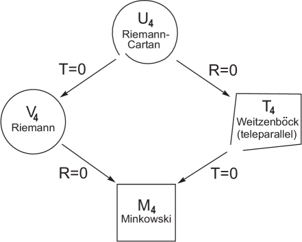
Figure 5.1: Riemann–Cartan (RC) space and its subcases. Torsion is denoted by $T$ and curvature by $R$.

5.2 Matter fields in the RC-arena

We consider matter fields $\Psi(x)$, typically a Dirac field, as “moving” in the RC-arena; see Chapter 4 and the [Reprints 5.1, 5.2, 5.3]. Their Lagrangian is assumed to couple minimally to the geometry: $L_{\text{mat}}=L_{\text{mat}}(g_{\alpha\beta},\vartheta^{\alpha},D\Psi)$. If their action, $\int L_{\text{mat}}$, is invariant under local Poincaré transformations, their canonical (Noether) currents of energy-momentum, $\mathfrak{T}_{\alpha}$, and spin angular momentum, $\mathfrak{S}_{\alpha\beta}$, arise as coupled to coframe and Lorentz connection, respectively. They fulfill the Noether identities

$$D\mathfrak{T}_{\alpha}=(e_{\alpha}\lrcorner T^{\beta})\wedge\mathfrak{T}_{\beta}+(e_{\alpha}\lrcorner R^{\beta\gamma})\wedge\mathfrak{S}_{\beta\gamma}\,,\qquad{D}\mathfrak{S}_{\alpha\beta}-\vartheta_{[\alpha}\wedge\mathfrak{T}_{\beta]}=0\,.$$ (5.1)

In flat spacetime, these are the conservation laws of energy-momentum and angular momentum.

Gauge potentials, $A$, of internal symmetries, because of the required internal gauge invariance, couple only to the coframe with their symmetric current, $\mathfrak{t}_{\alpha}\sim\delta L_{A}/\delta\vartheta^{\alpha}$. There is no direct coupling to torsion. Only in the case of a symmetry breakdown may the situation possibly change.

5.3 The two field equations of PG

The gravitational potentials are the orthonormal coframe, $\vartheta^{\alpha}$, and the Lorentz connection, $\Gamma^{\alpha\beta}$. Then the total Lagrangian reads:

$$L_{{\rm total}}=V(g_{\alpha\beta}\,,{\vartheta}^{\alpha}\,,{T^{\alpha}}\,,{R^{{\alpha}{\beta}}})\!+\!L_{{\rm matter}}(g_{\alpha\beta}\,,{\vartheta}^{\alpha}\,,{\Psi}\,,\stackrel{{\scriptstyle\Gamma}}{{D}}{\Psi})\,.$$ (5.2)

Define the translation and the Lorentz excitations (field momenta):

$${H_{\alpha}}=-\frac{{\partial}V}{{\partial}{T^{\alpha}}}\,,\qquad{H_{{\alpha}{\beta}}}=-\frac{{\partial}V}{{\partial}{R^{{\alpha}{\beta}}}}\,.$$ (5.3)

Then the Lagrange–Noether machinery yields the field equations [Reprint 5.1], [8]:

$$DH_{\alpha}-t_{\alpha}\hskip 6.0pt = {\mathfrak{T}_{\alpha}}\qquad\>\;\qquad\hskip 1.0pt(\text{{\sl First} = 1st field eq.\ of gravity by }{\delta}/{\delta}{\vartheta}^{\alpha})\,,$$

$$D{H_{{\alpha}{\beta}}}-s_{{\alpha}{\beta}} = \mathfrak{S}_{{\alpha}{\beta}}\qquad\qquad(\text{{\sl Second} = 2nd field eq.\ of gravity by }{\delta}/{\delta}{\Gamma}^{{\alpha}{\beta}})\,,$$

$$\frac{\delta L}{\delta\Psi} = 0\quad\qquad\hskip 1.0pt\qquad\;(\text{{\sl Matter} = matter field eq.\ by }{\delta/\delta\Psi})\,.$$

The energy-momentum, $t_{\alpha}:=\partial V/\partial\vartheta^{\alpha}$, and the spin, $s_{\alpha\beta}:=\partial V/\partial\Gamma^{\alpha\beta}$, of the gravitational gauge fields turn out to be

$$t_{\alpha}=e_{\alpha}\lrcorner V+(e_{\alpha}\lrcorner{T^{\beta}})\wedge{H_{\beta}}+(e_{\alpha}\lrcorner{R^{{\beta}{\gamma}}})\wedge{H_{{\beta}{\gamma}}}\,,\qquad s_{\alpha\beta}=-\vartheta_{[\alpha}\wedge H_{\beta]}\,.$$ (5.4)

These currents are gauge covariant three-forms, and they tell us about the energy and the spin “transported” by the gravitational gauge potentials $\vartheta^{\alpha}$ and $\Gamma^{\alpha\beta}$ themselves. Their existence is an expression of the universality of gravity.

Suppose—for a moment—that the gauge Lagrangian, $V$, does not depend on torsion, $T^{\alpha}$; then $H_{\alpha}=0$ and First collapses to $-t_{\alpha}=\mathfrak{T}_{\alpha}$; this is where the Einstein equation of GR is encapsulated. But now back to the general case.

Like in the Maxwell and the Yang–Mills theories, the gauge Lagrangian should be algebraic in $T^{\alpha}$ and $R^{\alpha\beta}$. Then we find second order partial differential equations (PDEs). Moreover, they should be quadratic in order to induce quasi-linearity of the PDEs, that is, linearity in the highest derivatives, here the second derivatives; as a consequence wave type field equations emerge. These two natural assumptions are very far-reaching. They are fulfilled in the theories of the strong and the electroweak interactions, and we will assume them here, too.

5.4 Gauge field theories of Abelian and non-Abelian groups compared

The Maxwell–Dirac theory as a $U(1)$ gauge field theory is Abelian. However, since the group $SU(2)$ is noncommutative, that is non-Abelian, the Yang–Mills theory is a nonlinear theory and its gauge current, ${\stackrel{{\scriptstyle A}}{{{I}}}}=-A\wedge H$, even though it is not gauge covariant, carries its own isospin, see Eq. (3.4).

The Poincaré group is also non-Abelian. Hence PG shares numerous properties with the Yang–Mills theory. The gauge currents carry their own charge and the theories become nonlinear. We would like to display the field equations (inhomogeneous and homogeneous ones) and the “constitutive relations” of the three theories mentioned:

Maxw: $$dH ={J}, dF =0, H =Y_{0}\,^{\star}\!F.$$

YM: $$\stackrel{{\scriptstyle A}}{{D}}{H} ={I}, \stackrel{{\scriptstyle A}}{{D}}{F} =0, H =\alpha_{0}\,^{\star}\!F.$$

PG1: $$\stackrel{{\scriptstyle\Gamma}}{{D}}H_{\alpha}-{t_{\alpha}} =\mathfrak{T}_{\alpha}, \stackrel{{\scriptstyle\Gamma}}{{D}}T^{\alpha} =R_{\beta}{}^{\alpha}\wedge\vartheta^{\beta}, H_{\alpha} =H_{\alpha}(T^{\gamma},R^{\delta\varepsilon});$$

PG2: $$\stackrel{{\scriptstyle\Gamma}}{{D}}H_{\alpha\beta}-{s_{\alpha\beta}} =\mathfrak{S}_{\alpha\beta}, \stackrel{{\scriptstyle\Gamma}}{{D}}R^{\alpha\beta} =0, H_{\alpha\beta} =H_{\alpha\beta}(T^{\gamma},R^{\delta\varepsilon}).$$

PG1 refers to the field equation related to translations and PG2 to the Lorentz rotations. The semi-direct product structure of $P(1,3)$ is reflected in the first Bianchi identity $DT^{\alpha}=\vartheta^{\beta}\wedge R_{\beta}{}^{\alpha}$ in the term $R_{\beta}{}^{\alpha}\wedge\vartheta^{\beta}$, mixing the Lorentz field strength with the translational potential; moreover, in First and Second the gauge currents $t_{\alpha}$ and $s_{\alpha\beta}$ contain mixing terms.

As in the Maxwell or in the Yang–Mills case, the field equations of the PG are second order PDEs in the potentials. If both $H_{\alpha}$ and $H_{\alpha\beta}$ are nonvanishing, they contain $\partial\vartheta$ and $\partial\Gamma$, respectively, as their leading derivative terms. We substitute them in the field equations and find (lhs = left-hand-side):

$$\text{lhs-{\sl First}}(\partial^{2}\vartheta,\partial\vartheta,\partial\Gamma,\vartheta,\Gamma) \sim \mathfrak{T}\,,$$ (5.5)

$$\vspace{5pt}\text{lhs-{\sl Second}}(\partial^{2}\Gamma,\partial\Gamma,\partial\vartheta,\Gamma,\vartheta) \sim \mathfrak{S}\,.$$ (5.6)

The initial value problem for (5.5) and (5.6) is related to the existence and uniqueness of the solution of a given partial differential equation for a set of consistently chosen initial data. In PG, with Lagrangians quadratic in the field strengths, the field equations are, as we saw, second order PDEs for the field variables. The integration of these equations consists of two separate steps: first, one defines the initial conditions as the set of constrained equations for the initial data (the values of fields and their first time derivatives on a 3d space-like hypersurface); and second, one solves the problem of temporal evolution for both the physical variables and the initial constraints. These considerations can be generalized to include matter fields.

Dimakis [10] analyzed, similar to Choquet-Bruhat and Bleecker in the EC case (see Chapter 4), the general parity preserving 10-parameter PG Lagrangian in vacuum. He found that the initial value problem is well-defined provided the parameters satisfy certain conditions. The physical meaning of these conditions is related to the existence of massive modes of the Lorentz connection $\Gamma^{\alpha\beta}$. The proof relies on the study of the field equations, the structure equations and the Bianchi identities, in combination with suitably chosen gauge conditions. A corresponding Hamiltonian analysis is discussed in Chapter 13.

A caveat should be stated before leaving this subsection. The gravitational gauge variables are the orthonormal coframe, $\vartheta^{\alpha}$, and the Lorentz connection, $\Gamma^{\alpha\beta}$. The Lagrangian, the field equations and the initial value problem are all stated in terms of these variables. To substitute the connection into the gauge Lagrangian according to $\Gamma^{\alpha\beta}=\widetilde{\Gamma}^{\alpha\beta}-K^{\alpha\beta}$, see Eq.(2.8), changes the order of the field equations and ruins the whole gauge structure. If one then takes derivatives of the torsion into the gauge Lagrangian, as done by Carroll and Field [11], then one finds something, but this has nothing to do with a gauge theory of gravity or with interpreting the torsion as the translational gauge field strength. Such an act of violence deprives the torsion of its native geometrical character.

A consistent change of gravitational field variables can be executed on the level of the Lagrangian by introducing suitable constraints via a Lagrange multiplier method, see [5], Sec. 5.8.

5.5 Einstein–Cartan theory as a degenerate Poincaré gauge theory

We restricted ourselves to gauge Lagrangians that are (i) algebraic and (ii) quadratic in torsion $T^{\alpha}$ and curvature $R^{\alpha\beta}$. Thus, the “constitutive relations” $H_{\alpha}=H_{\alpha}(T^{\gamma},R^{\delta\varepsilon})$ and $H_{\alpha\beta}=H_{\alpha\beta}(T^{\gamma},R^{\delta\varepsilon})$ are linear in these variables; for a specific example, see [Reprint 5.1], Eqs. (5.1) and (5.2). Accordingly, investigations into the most general linear constitutive equations are required in order to check which possibilities exist for a consistent PG.

However, we first want to look into two possible degenerate cases. If the translational excitation vanishes, $H_{\alpha}=0$, then the two gauge field equations read

$$-e_{\alpha}\lrcorner V-(e_{\alpha}\lrcorner{R^{{\beta}{\gamma}}})\wedge{H_{{\beta}{\gamma}}} = \mathfrak{T}_{\alpha}\,,$$ (5.7)

$$D{H_{{\alpha}{\beta}}} = \mathfrak{S}_{{\alpha}{\beta}}\,.$$ (5.8)

The simplest subcase of this class of models, namely $H_{\alpha\beta}=\frac{1}{\kappa}\eta_{\alpha\beta}=\frac{1}{\kappa}\,^{\star}(\vartheta_{\alpha}\wedge\vartheta_{\beta})$, leads back to the EC field equations (4.5) and (4.6). The degenerate character of this system becomes obvious if we look at the structure of the field equations:

$$\text{lhs-{\sl First}${}_{\rm EC}$}(\partial\Gamma,\Gamma,\vartheta) \sim \mathfrak{T}\,,$$ (5.9)

$$\vspace{5pt}\text{lhs-{\sl Second}${}_{\rm EC}$}(\partial\vartheta,\vartheta,\Gamma) \sim \mathfrak{S}\,.$$ (5.10)

In each variable one derivative order is lost when compared to (5.5) and (5.6), and the rotational field strength is proportional to the translational current and vice versa.

5.6 Translational gauge theory (TG) as another degenerate PG

A second degenerate case occurs when the Lorentz excitation vanishes, $H_{\alpha\beta}=0$ [Reprint 5.1]. Then, the gravitational Lagrangian does not depend on the curvature, $R^{\alpha\beta}$, and we can read off the corresponding field equations from First and Second. They turn out likewise to be independent of $R^{\alpha\beta}$. Accordingly, the field equations cannot control $R^{\alpha\beta}$. This is unsatisfactory from a physical point of view and cannot be tolerated. Thus, in order to formulate a well-defined theory, we require by hand the vanishing of the curvature, $R^{\alpha\beta}=0$.

For this purpose, we add to the curvature-free Lagrangian a Lagrange multiplier term, $-\frac{1}{2\varrho}\Lambda_{\alpha\beta}\wedge R^{\alpha\beta}$, and we find three field equations. The third one is the teleparallelism condition, $R^{\alpha\beta}=0$, that is, the spacetime now obeys a Weitzenböck geometry, see Fig. 5.1. If we then substitute $R^{\alpha\beta}=0$ into the first field equation, all terms containing the Lagrange multiplier vanish. In this way, we find [8]:

$$DH_{\alpha}-e_{\alpha}\lrcorner V+(e_{\alpha}\lrcorner T^{\beta})\wedge H_{\beta} = \mathfrak{T}_{\alpha}\,,$$ (5.11)

$${\frac{1}{2\varrho}}D\Lambda_{\alpha\beta}+\vartheta_{[\alpha}\wedge H_{\beta]} = \mathfrak{S}_{\alpha\beta}\,.$$ (5.12)

Eq. (5.12) only plays a subsidary role. It only determines the Lagrange multiplier two-form $\Lambda_{\alpha\beta}$. This is of no further interest since $\Lambda_{\alpha\beta}$ doesn’t occur in (5.11). Note that our method reintroduced the Lorentz excitation via the backdoor: $H_{\alpha\beta}=\frac{1}{2\varrho}\Lambda_{\alpha\beta}$. If we choose a global reference frame in which $\Gamma^{\alpha\beta}$ vanishes—this is always possible in a Weitzenböck spacetime—the left-hand-side of (5.11) depends only on the variables $(\partial^{2}\vartheta,\partial\vartheta,\vartheta)$; it is apparently the gauge field equation of the translation group. Note that the explicit form of the torsion-square Lagrangian has not been used so far. We will come back to its analysis in Chapter 6.

5.7 Most general quadratic PG Lagrangian with even and odd parity terms

Instead of following the detailed history of this expression, we refer to [Reprint 5.3], where this most general quadratic Lagrangian is discussed. The terms involved were already found by Obukhov et al. [12]. However, they dropped the parity violating pieces without further discussion. The complete Lagrangian was revived and applied to cosmology in [Reprint 5.3]. Diakonov et al. [13], in the course of quantum field theoretical considerations of gravity, investigated torsion and curvature-dependent Lagrangians in an RC-spacetime. One piece of their Lagrangian coincides with the quadratic one of [Reprint 5.3]. This was shown in detail by Baekler and Hehl [14]. For reference purposes, we display the most general quadratic Lagrangian, see [14], Eq. (56):

$$V = \,\frac{1}{2\kappa}\left[\,(\,a_{0}R+{b_{0}}X\phantom{\frac{1}{2}}-2\Lambda_{0})\,\eta\right.$$ (5.14)

$$\hskip 13.0pt\left.+\frac{a_{2}}{3}{\cal V}\wedge{}^{\star\!}{\cal V}-\frac{a_{3}}{3}{{\cal A}\wedge{}^{\star\!\!\!}{\cal A}}-\frac{2{\sigma}_{2}}{3}{{\cal V}\wedge{}^{\star\!\!\!}{\cal A}}+a_{1}{}^{(1)}T^{\alpha}\wedge{}^{\star(1)}T_{\alpha}\right]$$

$$-\frac{1}{2\varrho}\left[\Big{(}\frac{w_{6}}{12}R^{2}-\frac{w_{3}}{12}{X^{2}}+\frac{\mu_{3}}{12}RX\Big{)}\,\eta+w_{4}{}^{(4)}\!R^{\alpha\beta}\wedge{}^{\star(4)}\!R_{\alpha\beta}\right.$$

$$\left.+{}^{(2)}\!R^{\alpha\beta}\wedge\Big{(}w_{2}{}^{\star(2)}\!R_{\alpha\beta}+\mu_{2}{}^{(4)}\!R_{\alpha\beta}\Big{)}+{}^{(5)}\!R^{\alpha\beta}\wedge\Big{(}w_{5}{}^{\star(5)}\!R_{\alpha\beta}+\mu_{4}{}^{(5)}\!R_{\alpha\beta}\Big{)}\right].$$

The first two lines represent weak gravity, with the gravitational constant $\kappa$, the last two lines strong gravity with the dimensionless strong gravity constant $\varrho$. The parity odd pieces are those with the constants $b_{0},\sigma_{2};\mu_{2},\mu_{3},\mu_{4}$. In a Riemann space (where $X=0$), only two terms of the first line and two terms in the third line survive. All these four terms are parity even, that is, only torsion brings parity odd pieces into the gravitational Lagrangian. A Lagrangian with the first two terms $\sim\,a_{0}R+{b_{0}}X$ was first discussed by Hojman et al. [15].

It will be a task in the future to single out of this set of Lagranians (5.14) the physically acceptable one. Quite early, Blagojević and Nikolić [16] and Blagojević and Vasilić [Reprint 13.1] investigated the parity even quadratic Lagrangian and its consistent Hamiltonian prepresentation. More recently, progress in this direction for Lagrangians carrying parity odd pieces has been achieved, inter alia, by Yo & Nester [17] and in [18] and [Reprint 5.3] with theoretical methods, and by Li et al. [19, 20] mainly with numerical methods. Lately, Adak [21] coupled a Dirac electron non-minimally to the weak part of the Lagrangian (5.14).

5.8 Issues of interpretation

The analogies between PG and gauge theories of internal groups are very deep, and the name Poincaré gauge theory (of gravity; PG) seems justified to us. It is clear that the translation group is fairly unique in that it mediates between neighboring points in spacetime, quite in contrast to internal groups, which act at one point alone. Accordingly, it is not so surprising that the coframe, $\vartheta^{\alpha}$, as translational type potential does not have the inhomogeneous transformation law traditionally obeyed by potentials. Still, it couples decently to the translational current, the energy-momentum current $\mathfrak{T}^{\alpha}$, as a potential is supposed to do.

In spite of the undeniable success of the Sciama–Kibble approach, see Obukhov [23] and [24, 25], there have been different opinions regarding the question of whether and in what sense gravitation is a gauge theory. A precise mathematical analysis of the gauge content of PG reveals certain structural differences with respect to the Yang–Mills theories. The most difficult piece in this analysis is certainly the interpretation of local translations, which act not only on the fields, but also on the spacetime points. Trautman [26] defines a gauge theory as “any physical theory of a dynamical variable which, at the classical level, may be identified with a connection on a principal bundle”. Then, he continues with the statement: “In this sense, gravitation is a gauge theory …”. We should note in passing that many authors do not care about the conserved currents that we put at center stage of our considerations in formulating the gauge procedure.

Looking at the literature on the gauge structure of gravity, see Chapter 6 and [27], one can find convincing arguments that the Poincaré gauge approach, supported by the improved interpretation of its gauge structure, defines a consistent framework for studying gravitational dynamics in the realm of the RC-geometry of spacetime.

5.9 On torsion singularities

The early work on torsion singularities, see [28] and references given therein, can be epitomized by the title of Trautman’s article, “Spin and torsion may avert gravitational singularities”. But the singularities treated so far are only singularities of the metric induced by torsion-square pieces. Real torsion singularities, basically independent of the metric, were first studied by Nester and Isenberg [29]. Later, a number of papers appeared on torsion singulaities [30], but up to now the general situation is still somewhat opaque to us. More work seems necessary.

This chapter was devoted to the basic aspects of the Poincaré gauge approach to gravity. One degenerate case, EC-theory, was already treated in the last chapter; another one, the translational gauge theory, will be discussed in Chapter 6. Physical predictions of PG are presented in some detail in Chapters 13 to 16.

Chapter 6     Translational Gauge Theory

Reprinted papers:

• G. D. Kerlick, Spin and torsion in general relativity: foundations, and implications for astrophysics and cosmology, Ph.D. thesis (Princeton University, Princeton, NJ, January 1975); extract, pp. 39–49.

• J. M. Nester, Gravity, torsion and gauge theory, in: H. C. Lee (ed.), An Introduction to Kaluza–Klein Theories (World Scientific, Singapore, 1984), pp. 83–115; extract, pp. 89–92.

• Y. Itin, Energy-momentum current for coframe gravity, Class. Quantum Grav. 19, 173–189 (2002); extract, pp. 175–181, 189.

The general geometric arena of Poincaré gauge theory, the Riemann–Cartan space, $U_{4}$, may be restricted a priori by imposing certain conditions on the curvature and/or the torsion. Thus, Einstein’s GR is defined in a Riemannian space, $V_{4}$, obtained from a $U_{4}$ by the requirement of vanishing torsion, whereas a complementary limit, the Weitzenböck or teleparallel space, $T_{4}$, is defined by the requirement of vanishing curvature (Fig. 5.1). The vanishing of curvature means that parallel transport is path independent (if some topological restrictions are adopted), hence we have a space with absolute (or tele)parallelism.

The mathematical analysis of the teleparallel geometry started with Weitzenböck (1923) and Cartan (1923/24), but it was Einstein (1928) who introduced this geometry into physics, in an (unsuccessful) attempt to unify gravitation and electromagnetism. The first period of teleparallelism was closely connected to unified field theory, and it lasted for about 10 years [1, 2]. In the 1960s, Møller and others revived the idea of teleparallelism as a dualistic field theory by moving its interpretation to a different stage: it became the geometric basis for a new, teleparallel theory of gravity interacting with matter, which turned out to be a possible alternative to GR [Reprint 5.1]. This represents the second (and still ongoing) period of the teleparallelism; for a textbook presentation, see Blagojević [3] and Ortín [4]. In this chapter, we focus our attention on this new interpretation of teleparallelism and its relation to the translation gauge theory of gravity (TG). Such a relation in regard to Møller’s tetrad theory of gravitation was established in [5].

The general form of the field equation for TG is given in Eq. (5.11) and was first derived in [Reprint 5.1], Eq. (6.10). A modern and concise presentation of the main results of TG, all explicitly calculated, is given in [Reprint 6.3], see also [6].

6.1 Gauging the translations

In the early 1960s, gauge theories of spacetime symmetries were developed starting with the Poincaré group, $P(1,3)$, as the group of rigid symmetries of a matter Lagrangian in Minkowski spacetime, $M_{4}$. While the gauge structure of the Lorentz sector $SO(1,3)$ of $P(1,3)$ is essentially the same as in Yang–Mills theories, the situation with translations $T(4)$ is rather different.

Motivated by the usual Yang–Mills formalism, Kibble [Reprint 4.2] treats translations as follows. At a point with coordinates $x=(x^{\mu})$, he defines the covariant derivative by adding the usual compensating field term to the partial derivative, $\nabla_{\mu}:=\partial_{\mu}+A_{\mu}{{}^{\nu}}P_{\nu}$, see also [7]. Then, using $P_{\nu}=-\partial_{\nu}$, he obtains $\nabla_{\mu}=h_{\mu}{{}^{\nu}}\partial_{\nu}$, with

$$h_{\mu}{{}^{\nu}}:=\delta_{\mu}^{\nu}-A_{\mu}{{}^{\nu}}\,.$$ (6.1)

Further analysis of the geometric meaning of $h_{\mu}{{}^{\nu}}$ leads to a consistent change of the notation $h_{\mu}{{}^{\nu}}\to h_{i}{{}^{\nu}}$, where $i$ is a local Lorentz index and $h_{i}=h_{i}{{}^{\nu}}\partial_{\nu}$ is the set of four orthonormal vectors, the tetrad. Equation (6.1) provides a link between the geometric and gauge content of local translations, but, nevertheless, the relation between general coordinate transformations and local translations remains somewhat unclear. Some aspects of this important issue are discussed in [Reprints 6.1, 6.2].

The action of the group $T(4)$ on the points of spacetime and the physical fields can be described as follows: (i) $T(4)$ moves a point at $x$ to the new position $x^{\prime}=x+\xi$ (the action on the base space); (ii) for every $x$, $T(4)$ acts on a field $\phi(x)$ by changing its form, $\phi(x)\to\phi^{\prime}(x)=\phi(x)-\xi^{\rho}\partial_{\rho}\phi(x)$ (the action on a fiber). It is the first action by which gauge theories of spacetime symmetries differ from the Yang–Mills theories [8]. This difference is often expressed by saying that the tetrad field is not the compensating field of the Yang–Mills type, but its precise mathematical description can be given in the fiber bundle formalism [9]. In the words of Dass [10], “the correct treatment of gauged translations should be in terms of translational connections and not general coordinate transformations on the base manifold”. A treatment of this kind was proposed by Cho [11], but, insisting on the local Lorentz invariance of the resulting theory, he ended up not with a genuine translational gauge theory but with the standard GR. Using the same approach, Dass was able to recognize the objects that are to be identified with the (invertible) tetrad fields. In [12], the authors use the technique of nonlinear realizations to discuss gauge theories of spacetime symmetries containing translations. Applying this approach, they are able to identify the tetrad field as a piece of the general nonlinear connection. Equation (6.1) represents a simplified version of this identification.

6.2 The embedding technique

The condition of vanishing curvature in an RC-spacetime can be imposed by using the method of Lagrange multipliers, see [13], Sec. 5.9, which implies that the Lorentz connection is trivial, but not necessarily zero. On the other hand, in the gauge theory of $T(4)$, we have an identically vanishing Lorentz connection. Is the first approach to TG in any way superior to the second one? Obukhov and Pereira [14] studied a similar embedding of TG in metric-affine gravity and noted that the first approach leaves more freedom in the choice of a convenient reference frame. In particular, they used this freedom to simplify the construction of some specific classical solutions. Similar conclusions were derived from the study of conserved charges in TG embedded in Poincaré gauge theory [15]. Using a trivial but non-vanishing connection, the authors were able to find the conservation laws not only for energy-momentum but also for angular momentum.

6.3 Observational predictions

In the realm of an RC-geometry, the teleparallel theory is characterized by the trivial Lorentz connection, so that the corresponding gauge structure corresponds to the translational gauge theory, with torsion as the only non-vanishing field strength. Demanding parity invariance, the standard Lagrangian of the theory is given as a sum of the squares of three irreducible parts of the torsion. The physical interpretation of TG is based on the following observations, see [Reprint 5.1] and [16, 17].

(a) There is a one-parameter family of teleparallel Lagrangians, $L_{\rm T}^{(\lambda)}$, defined by a single coupling constant, $\lambda$,

$$L_{\rm T}^{(\lambda)}=L_{\rm HE}+\lambda\,{\rm(axial~{}torsion)}^{2}\,+\,{\rm divergence}\,,$$ (6.2)

which is empirically equivalent to GR in linear approximation. Moreover, the Schwarzschild solution is also a solution of the one-parameter teleparallel theory, whereas all the observational differences with respect to GR stem from the term proportional to $\lambda$.

(b) For $\lambda=0$, $L_{\rm T}^{(\lambda)}$ reduces, up to a divergence, to the Hilbert–Einstein Lagrangian and becomes invariant under local Lorentz transformations. The resulting theory is usually called the teleparallel equivalent of GR (GR_∥) and is equivalent to GR for scalar, Maxwell and classical fluid matter. For spinor matter the Lorentz group needs to be gauged additionally and consequently, one should turn to PG generally, or to EC specifically.

Observable differences between TG and GR can be found by studying the motion of test objects in these theories (Chapter 14). For an interesting analysis and the geometric interpretation of some simple gravitational effects in terms of the torsion field, see [18].

6.4 Is the time evolution of torsion determined?

For some time, the one-parameter teleparallel theory has been a promising alternative to GR. However, analyzing this theory, Kopczyński [19] found a hidden gauge symmetry, which led him to the conclusion that the torsion evolution is not completely determined by the field equations (together with initial data). He argued that, since the torsion should be a measurable quantity, the theory is internally inconsistent. Later, Nester [20] improved the arguments of Kopczyński; the evolution problem was stated more precisely and bound to certain very special solutions. This conclusion has been further verified by Cheng et al. [21], who recognized the importance of nonlinear constraint effects for the dynamical structure of the theory. Investigating the initial-value problem, Hecht et al. [22] found that in vacuum the only consistent choice of the teleparallel Lagrangian corresponds to GR_∥. However, the coupling of a Dirac field in GR_∥ is not consistent [3, 14]. In order to improve this situation, Andrade et al. [23] suggested that the trivial Lorentz connection should be replaced by the Riemannian one, but this modification ignores the fact that each geometry has its own fundamental connection, which, in our opinion, should be an intrinsic part of the gauge approach to gravity.

The teleparallel geometry of GR_∥ was used to formulate a pure tensorial proof of the positivity of energy for Einstein’s theory [24], and to give a transparent description of Ashtekar’s complex variables [25]. Thus, GR_∥ is an extremely useful reformulation of the standard GR. However, when one studies the gravitational interaction of the Dirac field, one arrives at inconsistencies. Namely, the “main” field equation, obtained by varying the Lagrangian with respect to the tetrad field, implies that the antisymmetric part of the dynamic energy-momentum tensor vanishes, which is not true for the Dirac field. Problems of this kind were to be expected, since the Lorentz part of $P(1,3)$, which is important for spinors, was not gauged.

Thus, according to our present understanding, the only consistent version of the teleparallel theory is GR_∥ in interaction with scalar field, with Maxwell and nonabelian Yang–Mills fields, and also with classical fluid matter. Excluding the nonabelian Yang–Mills fields, one can think of GR_∥ as an effective theory of the macroscopic gravitational phenomena, equivalent to GR. However, all the problematic features of the teleparallel theory become irrelevant by turning, as one should, to the full Poincaré gauge theory.

Chapter 7     Fallacies About Torsion

Reprinted papers:

• B. Gogala, Torsion and related concepts: an introductory overview, International Journal of Theoretical Physics 19, 573–586 (1980); extract, pp. 573–583, 586

R. P. Feynman: It ain’t that simple. You got to look at things physically, see! You got these particles, and they attract each other, see. They bounce photons off each other, they get closer, and they go round each other, see! It’s a kind of screwing motion (illustrative gesture). The situation gets real complicated. You got to try to think of it physically. You can’t describe all this by just one word: TOISION.

B. S. DeWitt: Are there any questions?

(All rise and speak simultaneously)

Extract from the play presented at the concluding dinner of [1].

In the year 1962, during the general relativity conference in Warsaw [1], Ivanenko spoke on the importance of torsion in gauge theories of gravitation. Feynman interrupted him twice and asked him about the meaning of the concept of torsion. Ivanenko’s answer was not very specific. In particular, he linked torsion to Lorentz transformations, disregarding its character as a translational field strength. This was perhaps excusable since the 1961 paper by Kibble [Reprint 4.2] was probably not known at the conference. Anyway, the after dinner play probably expressed Feynman’s mood about torsion appropriately; see, however, his recognition [Reprint 3.5] in 1962/63 of the translation group as fundamental to gravity.

Of course, since the advent of Kibble’s paper in 1961 the mood should have changed. In fact, it did, but not to the extent we would have expected. There are still numerous critical statements in the literature about the torsion of spacetime that do not stand up to a closer examination. Let us quote some examples.

7.1 Wishful thinking of Landau–Lifshitz (1962)

Does the torsion really vanish? The authors of [3] consider on p. 279 a vector field $A_{i}$ that is the gradient of a scalar field. Starting with the correct formula,

$$D_{i}A_{k}-D_{k}A_{i}=\left({\mit\Gamma}^{\ell}_{ik}-{\mit\Gamma}^{\ell}_{ki}\right)A_{\ell}\,,\qquad A_{i}:=\partial_{i}\phi\,,$$ (7.1)

they continue on p. 280: “In a cartesian coordinate system the covariant derivative reduces to the ordinary derivative, and therefore the left side of our equation becomes zero. But since $D_{i}A_{k}-D_{k}A_{i}$ is a tensor, then being zero in one system it must also be zero in any coordinate system. Thus, we find that…” ${\mit\Gamma}^{i}_{k\ell}={\mit\Gamma}^{i}_{\ell k}$, which means that the torsion tensor has to vanish.

Can one really find a coordinate system in which $\nabla_{i}=\partial_{i}$ and, consequently, ${\mit\Gamma}^{i}_{k\ell}=0$ (at a given point of spacetime)? On the same page, there is the well-known formula for transforming ${\mit\Gamma}$ from one coordinate system to another. Using this formula, one finds that by a suitable coordinate transformation, one can make only the symmetric piece of $\,{\mit\Gamma}$ vanish. Note that this result is not valid for frame transformations, see Eq. (7.4). Therefore, if the original ${\mit\Gamma}$ is assumed to be asymmetric, one cannot prove that there is a coordinate system in which ${\mit\Gamma}=0$, and thus one cannot prove that ${\mit\Gamma}$ is symmetric, that is, that the torsion vanishes.

Nonmetricity. Of similar quality is the argument on p. 281 in regard to the vanishing of $D_{\ell}g_{ij}$. Namely, the authors start by stating that “the relation $DA_{i}=g_{ik}DA^{k}$ is valid for the vector $DA_{i}$, as for any other vector”. But $DA_{i}$ is not a vector, as is clear from the component form of the above equation:

$$D_{\ell}A_{i}=g_{ik}D_{\ell}A^{k}\,.$$ (7.2)

Comparing this relation with the general formula (given on the same page),

$$D_{\ell}A_{i}=D_{\ell}(g_{ik}A^{k})=(D_{\ell}g_{ik})A^{k}+g_{ik}D_{\ell}A^{k}\,,$$ (7.3)

one concludes that Eq. (7.2) is based on the assumption $D_{\ell}g_{ik}=0$, which is exactly what the authors intend to prove. Thus, the proof that $D_{\ell}g_{ik}=0$ is derived by assuming implicitly that $D_{\ell}g_{ik}=0$! Logically, as in the proof with the torsion, this is circular reasoning and thus incorrect; it is in both cases a petitio principii.

7.2 Misner–Thorne–Wheeler (1973): Vanishing torsion by
drawing

In the index of Misner, Thorne and Wheeler (MTW) [4] there is an entry, “Torsion not present in affine connection if equivalence principle is valid, 250”. If one turns to page 250, the first thing one observes is that the figure under the heading “ ‘Symmetry’ of covariant differentiation” is incorrectly drawn. Thus, MTW display an incorrect drawing and use it for their reasoning on torsion. Contrary to what they state, torsion survives the equivalence principle untouched, as had been earlier discussed by Sciama [Reprint 4.1].

Gogala [Reprint 7.1] corrected MTW’s figure, see also Nester [5], Fig. 1, and Gronwald and Hehl [6], Fig. 4. In the corrected figure, an additional translation shows up, induced by the torsion, thus invalidating the proof of MTW.

7.3 Ohanian & Ruffini (1994): Cracked parallelograms and
genuine spin

A cracked parallelogram doesn’t destroy local Euclidicity. Ohanian and Ruffini claim that the Einstein–Cartan theory is defective, see [7], pp. 311 and 312:

If $\,\Gamma^{\beta}{}_{\nu\mu}$ were not symmetric, the parallelogram would fail to close. This would mean that the geometry of the curved spacetime differs from a flat geometry even on a small scale—the curved spacetime would not be approximated locally by a flat spacetime.

Let us look at the geometrical facts. Locally, a Riemann–Cartan (RC) space looks Euclidean, since for any single point, $P$, there exist coordinates, $x^{i}$, and an orthonormal coframe, $\vartheta^{\alpha}$, such that

$$\left\{\begin{array}[]{rcl}\vartheta^{\alpha}&=&\,\delta^{\alpha}_{i}dx^{i}\\ \Gamma_{\alpha}{}^{\beta}&=&\,0\end{array}\right\}\quad{\rm at}\,\,\,P\,,$$ (7.4)

where $\Gamma_{\alpha}{}^{\beta}$ are the connection 1-forms referred to the coframe $\vartheta^{\alpha}$, see Hartley [8] for details. Eq. (7.4) represents, in an RC-space, the anholonomic analogue of the (holonomic) Riemannian normal coordinates of a Riemannian space.

Equation (7.4) disproves the Ohanian and Ruffini statement right away. In (7.4) it is clearly displayed that the RC geometry is Euclidean in the infinitesimal, and this was even one of the guiding principles of Cartan for generalizing the Minkowski spacetime and his reason to call the emerging connection of an RC-space an “Euclidean connection”.

“Genuine” spin. In a footnote on page 312 we read inter alia:

Cartan’s modification of Einstein’s theory attempts to take the spin density of elementary particles as the source of torsion. But this introduces ambiguities because we do not know the ‘genuine’ spin content of elementary particles—for instance, we do not know the internal structures of quarks, and we are therefore unable to say whether their ostensible spin $\hbar/2$ is genuine spin, or a combination of spin and orbital angular momentum of the constituents (if any) within the quarks…

Let us turn a bit closer to gravitational experiments. In the COW-experiment, discussed in Chapter 4, a coherent neutron wave moves in a gravitational field. It is an experimental fact that the neutron has spin $\hbar/2$, as discussed in detail by Alexandrov [9], for example. Of course it is not known how much orbital and how much intrinsic angular momentum of the three quarks contribute to the spin $\hbar/2$ of the neutron. But this doesn’t affect the validity of the Dirac equation for the neutron, which is non-minimally coupled to the electromagnetic and gravitational fields because of its composed nature. In the low energy regime, realized in the COW-interferometer, the non-relativistic Schrödinger–Pauli equation, approximating the Dirac equation, is all we need. In PG in general and in EC particularly, the source of the second field equation of gravity is the canonical spin that can be calculated according to the Noether procedure from the Dirac field. As long as the neutron obeys a Dirac equation, the qualms of Ohanian and Ruffini are irrelevant. We search for the canonical spin, not for a mysterious “genuine” spin, perhaps hidden deep inside matter.

According to present day wisdom, matter is built up from quarks and leptons. No substructures have been found so far. According to the mass-spin classification of the Poincaré group and the experimental information of lepton and hadron collisions etc., leptons and quarks turn out to be fermions with spin 1/2 (obeying the Pauli principle). As long as we accept the (local) Poincaré group as a decisive structure for describing elementary particles, there can be no doubt what spin really is (Wigner 1939). Abandoning the Poincaré group would also result in an overhaul of the (locally valid) special relativity theory.

7.4 Kleinert & Shabanov (1998): Scalar particles and
autoparallels

Kleinert and Shabanov [10] postulate that a scalar particle moves in a Riemann–Cartan space along an autoparallel. However, the equations of motion cannot be postulated freely; rather, they have to be determined from the energy-momentum and the angular momentum laws of the underlying theory. It turns out that a scalar particle can only “feel” the Riemannian metric of spacetime, it is totally insensitive to a possibly existent torsion (and nonmetricity) of spacetime, see Chapter 14, conclusion (i) and the proof given there. Torsion can only be detected by using test bodies composed of elementary particles with nonvanishing intrinsic spin.

7.5 Carroll (2004): Torsion not distinguished from other
tensor fields

Carroll [11] argues on p. 190 of his book as follows:

As a final alternative to general relativity, we should mention the possibility that the connection really is not derived from the metric, but in fact has an independent existence as a fundamental field… We could drop the demand that the connection be torsion-free, in which case the torsion tensor could lead to additional propagating degrees of freedom. The basic reason why such theories do not receive much attention is simply because the torsion is itself a tensor; there is nothing to distinguish it from other, nongravitational tensor fields. Thus, we do not really lose any generality by considering theories of torsion-free connections (which lead to GR) plus any number of tensor fields, which we can name what we like. Similar considerations apply when we consider dropping the requirement of metric compatibility—any connection can be written as a metric-compatible connection plus a tensorial correction, so any such theory is equivalent to GR plus extra tensor fields, which wouldn’t really deserve to be called an “alternative to general relativity”.

(i) This opinion is often expressed by particle physicists who have a somewhat relaxed relation towards differential geometry. The torsion tensor is not any tensor, but a particular tensor related to the translation group. A torsion tensor cracks infinitesimal parallelograms. A parallelogram is deeply related to the geometry of a manifold carrying a linear connection. The closure failure of a parallelogram can only be created by a distinctive geometrical quantity, namely the torsion tensor, and not by any other tensor. This fact alone makes Carroll’s argument defective.

Needless to say that the incorrect drawing of MTW reemerges in Carroll [11] on page 122. So much for a proper geometric understanding of torsion and about independent thinking.

(ii) Another, more formal way of saying the same thing is that torsion affects the Bianchi identities. Namely, if we differentiate torsion, $T^{\alpha}$, and curvature, $R_{\alpha}{}^{\beta}$, we find straightforwardly the first and the second Bianchi identities, respectively:

$$DT^{\alpha}=R_{\beta}{}^{\alpha}\wedge\vartheta^{\beta}\,,\qquad DR_{\alpha}{}^{\beta}=0\,.$$ (7.5)

We can recognize how closely torsion and curvature are interrelated. It is apparent that torsion as well as curvature are notions linked to the process of parallel displacement on a manifold and are, as such, of a very particular nature. Moreover, as we saw already in Chapter 5, the torsion is the field strength belonging to one particular group, namely the translation group.

(iii) As Sciama [Reprint 4.1] has shown, an independent Lorentz connection couples to the spin current of a matter field in a similar way as the coframe couples to the energy-momentum current of matter. By splitting off the Levi-Civita part from the Lorentz connection, one deprives the spin current of matter from the potential it couples to. The splitting technique advised by Carroll ruins the whole gauge structure. Minimal coupling would lose its heuristic power.

(iv) In the paper by Carroll and Field [12], it is vividly shown to what odd consequences the philosophy of “torsion is like any other tensor field” leads: In order to make torsion propagating, they introduce derivatives of the torsion into their Lagrangian, in contrast to the doctrine of gauge theory. One should rather take a torsion-square Lagrangian, as we have demonstrated in Chapter 5.

7.6 Weinberg (2005): “Is there any physical principle …?”

Weinberg [13] wrote an article about “Einstein’s mistakes”. In a response, Becker [14] argued that for “generalizing general relativity” one should allow torsion and teleparallelism. Weinberg’s response [15] was as follows:

I may be missing the point of Robert Becker’s remarks, but I have never understood what is so important physically about the possibility of torsion in differential geometry. The difference between an affine connection with torsion and the usual torsion-free Christoffel symbol is just a tensor, and of course general relativity in itself does not constrain the tensors that might be added to any dynamical theory. What difference does it make whether one says that a theory has torsion, or that the affine connection is the Christoffel symbol but happens to be accompanied in the equations of the theory by a certain tensor? The first alternative may offer the opportunity of a different geometrical interpretation of the theory, but it is still the same theory.

How should one know, in GR, which tensor field to add to the Christoffel symbol, if one is not aware of the (geometric) minimal coupling procedure of PG?

Weinberg’s statement has already been answered by one of us, see [15]. We argued, as we do here, that torsion is related to the translation group and that it is, in fact, the translational gauge field strength. Moreover, we pointed out the existence of a new spin-spin contact interaction in the EC-theory and that torsion could be measured by the precession of the spin of elementary particles.

Weinberg’s answer was:

Sorry, I still don’t get it. Is there any physical principle, such as a principle of invariance, that would require the Christoffel symbol to be accompanied by some specific additional tensor? Or that would forbid it? And if there is such a principle, does it have any other testable consequences?

The physical principle Weinberg is looking for is translational gauge invariance, see Chapters 4 and 5. And the testable consequences are related to the new spin-spin contact interaction and to the precession of elementary particle spins in torsion fields.

7.7 Mao–Tegmark–Guth–Cabi (2007): Gravity Probe B and torsion

Mao, Tegmark, Guth, and Cabi [16] claim that torsion can be measured by means of the Gravity Probe B experiment. This is incorrect since the sensitive pieces of this gyroscope experiment, the rotating quartz balls, don’t carry uncompensated elementary particle spin, see also Ni [Reprint 4.4]. If the balls were made of polarized elementary particle spins, that is, if one had a nuclear gyroscope, see Simpson [17], as they were constructed for inertial platforms, then the gyroscope would be sensitive to torsion. As mentioned in the last point regarding Kleinert et al., an equation of motion in a general relativistic type of field theory has to be derived from the energy-momentum and angular momentum laws, see [Reprints 14.1, 14.2]. Then, it turns out that measuring torsion requires elementary spin, there is no other way. Orbital angular momentum is not a substitute for spin.

Would you use an electrically and magnetically neutral test particle for tracing possible electromagnetic fields? By the same token: Would you use a macroscopically rotating quartz ball of Gravity Probe B for tracing a possible torsion field?

Anyway, March et al. [18] continued the Mao et al. program, in particular they made “…use of the autoparallel trajectories, which in general differ from geodesics when torsion is present”. As we pointed out above, autoparallels have nothing to do with the motion of matter directly: if the matter is spinless, it moves along the Riemannian geodesics, if it carries spin, then the motion is not universal but depends on the initial orientation of its spin, for example, and an autoparallel cannot control its motion.

March et al. are aware of our objections and discuss them, but eventually they conclude that the Mao et al. framework “is adequate for the description of torsion around macroscopic massive bodies in the Solar System, such as planets, being the intrinsic spin negligible when averaged over such bodies”. No reason is given in favor of this adequacy.

7.8 Torsion in string theory?

Quite some time ago it was noticed by Scherk and Schwarz [19] that the low-energy effective string theory can be elegantly reformulated in geometrical terms by using a non-Riemannian connection. The graviton field, the dilaton field and the antisymmetric tensor field (2-form $B$), which represent the massless modes of the closed string, then give rise to a geometry with torsion and nonmetricity. In particular, the 3-form field $H=dB$ is often interpreted as torsion in this picture, see also Vasilić [20], who explained the relation between $dB$ and Cartan’s torsion. Later this idea was extended to interpret the dilaton field as the potential for the (Weyl) nonmetricity, see [21, 22, 23], for example. Looking for the definition of torsion in Polchinski’s book [24], we find in his glossary on page 514:

torsion a term applied in various 3-form field strengths, so called because they appear in covariant derivatives in combination with the Christoffel connection.

Thus, the notion of torsion in string theory is often used in an unorthodox and confusing way and should not be mixed up with Cartan’s torsion of 1922.

7.9 Torsion and electromagnetism?

In the past, there have been numerous failed attempts to relate the torsion of spacetime to electromagnetism, see the reviews of Tonnelat [25] and Goenner [26]. These failures can be well understood nowadays: As we have seen in Chapters 5 and 6, torsion is irresolvably tied to the translation group. Thus, torsion has nothing to do with internal (unitary) symmetry groups such as $U(1)$ (electromagnetism), $SU(2)$ (weak interaction) or $SU(3)$ (strong interaction). Still, again and again people make new attempts, see, for instance, Evans [27] and Poplawski [28]. It has been shown explicitly [29] that Evan’s theory is untenable.

x

Part C     Extending the Gauge Group of Gravity

Chapter 8     Poincaré Group Plus Scale Transformations:
Weyl–Cartan Gauge Theory of Gravity

Reprinted papers:

• W. Kopczyński, J. D. McCrea, and F. W. Hehl, The Weyl group and its currents, Phys. Lett. A 128, 313–317 (1988).

• J. M. Charap and W. Tait, A gauge theory of the Weyl group, Proc. Roy. Soc. Lond. A 340, 249–262 (1974).

• H. T. Nieh, A spontaneously broken conformal gauge theory of gravitation, Phys. Lett. A 88, 388–390 (1982).

In his reconsiderations of the foundations of geometry [1], Weyl started from the fundamental property of Euclidean geometry that the square of the distance between any two points is a quadratic form of their relative coordinates: ${\mit\Delta}s^{2}=g_{\mu\nu}{\mit\Delta}x^{\mu}{\mit\Delta}x^{\nu}$. However, by restricting our attention to the points that are infinitesimaly close to each other, with $ds^{2}=g_{\mu\nu}dx^{\mu}dx^{\nu}$, we enter the domain of Riemannian geometry. Inspired by Einstein’s general relativity, Weyl came to the conclusion that “…Riemann’s geometry goes only half-way towards attaining the ideal of a pure infinitesimal geometry … Riemann assumes that it is possible to compare the lengths of two line elements at different points of space, too" ([1], p. 102). Thus, the transition to $ds^{2}$ is only a first step to a truly “infinitesimal" geometry; the second step, the one that remained unrealized in Riemannian geometry, consists of allowing a non-Euclidean “recalibration" of spacetime, in which the measure of length will not remain fixed under a parallel transport [1, 2, 3, 4].

8.1 Weyl geometry

For a vector, $V$, with the measure of length $V^{2}=g_{\mu\nu}V^{\mu}V^{\nu}$, Weyl’s new calibration is defined by the semi-metric condition

$$DV^{2}=V^{2}\varphi\quad{\Leftrightarrow}\quad Dg_{\mu\nu}=\varphi g_{\mu\nu}\,,$$ (8.1a)

where $$D=dx^{\mu}D_{\mu} {\mit\Gamma} \varphi=\varphi_{\mu}dx^{\mu} V^{2} {\mit\Gamma}$$ is the exterior covariant derivative with respect to a new connection , and is a differential 1-form independent of . Assuming the connection to be symmetric implies

$${\mit\Gamma}^{\mu}{}_{\nu\rho}=\bar{\mit\Gamma}^{\mu}{}_{\nu\rho}-\frac{1}{2}\left(\delta^{\mu}_{\nu}\varphi_{\rho}+\delta^{\mu}_{\rho}\varphi_{\nu}-g_{\nu\rho}\varphi^{\mu}\right)\,,$$ (8.1b)

where $\bar{\mit\Gamma}^{\mu}{}_{\nu\rho}=\{\stackrel{{\scriptstyle\mu}}{{{}_{\nu\rho}}}\}$ is the Riemannian connection. The space defined by the metric, $g$, and the torsionless, symmetric connection, ${\mit\Gamma}$, is known as the Weyl space, $W_{4}$. In contrast to the Riemann space, $V_{4}$, the $W_{4}$ is characterized by a nonvanishing nonmetricity tensor, $Q_{\rho\mu\nu}:=-D_{\rho}g_{\mu\nu}$. More precisely, if we decompose $Q_{\rho\mu\nu}$ into a traceless and a trace part, $Q_{\rho\mu\nu}=Q\diagup_{\rho\mu\nu}+Q_{\rho}g_{\mu\nu}$, with $Q_{\rho}=\frac{1}{4}Q_{\rho\mu}{{}^{\mu}}$, the only piece that remains in a $W_{4}$ is the trace 1-form ${\rm tr}\hskip 1.00006ptQ=Q_{\rho}dx^{\rho}$ [5].

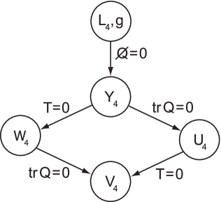
Figure 8.1: Weyl–Cartan geometry, $Y_{4}$, is the subclass of the metric-affine geometry $(L_{4},g)$, characterized by $Q\diagup=0$. Subcases are Weyl geometry, $W_{4}$, Riemann–Cartan geometry, $U_{4}$, and Riemann geometry, $V_{4}$.

By dropping the assumption that ${\mit\Gamma}$ is symmetric, one arrives at a more general result: the connection is again of the general form (8.1b), but now $\bar{\mit\Gamma}$ becomes a Riemann–Cartan connection, the general solution of the metricity condition, $\bar{D}g_{\mu\nu}=0$. Thus, ${\mit\Gamma}$ is a non-metric connection with torsion, which defines a Weyl–Cartan space, $Y_{4}$, or Weyl space with torsion [5, 6]. When compared to a $U_{4}$, a Weyl–Cartan spacetime incorporates recalibration of scale as a new kind of gauge symmetry. The new structure of spacetime can be thought of as a consistent extension of the $U_{4}$ by local scale invariance [7]. Weyl geometry is a special case of the metric-affine geometry, with the characteristic property $Q\diagup=0$ (Fig. 8.1). Accordingly, metric-affine geometry can be considered as a more satisfying realization of Weyl’s “infinitesimal" geometry, as already recognized by Einstein (see Chapter 9).

8.2 On the physical interpretation

Weyl formulated his results on the foundations of geometry in 1918, only two years after Einstein published his final version of GR. Relying on these post-Riemannian ideas, he tried to construct a unified field theory of gravity and electromagnetism, the only two known fundamental interactions at the time, by identifying $\varphi_{\mu}$ with the electromagnetic potential $A_{\mu}$. The construction was soon recognized as being unable to accommodate well-known properties of the electromagnetic interaction, since the Weyl potential, $\varphi_{\mu}$, is not coupled to the electric, but in fact to the dilatation current of matter, see [2, 5] and [Reprint 8.1]. Eleven years later, in his seminal paper [Reprint 2.3], Weyl succeeded in resurrecting and firmly establishing the gauge principle by deriving the electromagnetic interaction of the Dirac field from the gauging of the group $U(1)$. After that, Weyl’s 1918 attempts were almost forgotten, in spite of their deeply founded geometric content.

However, the situation changed in the late 1960s, when experimental results on deep inelastic electron-nucleon scattering focused physicists’ attention on theories that have no intrinsic scale (“Bjorken scaling"). Localization of the scale symmetry brings us back to the old Weyl theory that now doesn’t describe the electromagnetic, but rather a gravitational interaction of locally scale-invariant matter, originating from the dilatation current.

8.3 Weyl gauge theory

In the gauge approach to gravity, the central role belongs to matter and its rigid symmetries, and the geometric structure emerges in the process of localizing these symmetries. In [Reprint 8.2], Charap and Tait generalized the work of Kibble [Reprint 4.2] as a simple extension of the Poincaré group, the semi-direct product of $P(1,3)$ with the group of dilatations, denoted here as $W(1,3)$ and usually called the Weyl group.

The gauge procedure starts with a matter action integral, $I_{M}=\int{\cal L}_{M}(\phi,\partial_{i}\phi)d^{4}x$, in locally Minkowskian spacetime, which is invariant under the infinitesimal rigid Weyl transformations of the spacetime points, $\delta x^{\mu}=\varepsilon^{\mu}+\omega^{\mu}{{}_{\nu}}x^{\nu}+\rho x^{\mu}=:\xi^{\mu}$, the matter fields, $\phi$, and their partial derivatives, $\partial_{i}\phi$. These transformations are expressed in terms of 11 infinitesimal real parameters: 10 parameters $(\varepsilon^{\mu},\omega^{\mu\nu})$ define Poincaré transformations, and 1 parameter, $\rho$, defines dilatations. For a large class of theories, dilatations act on the fields according to $\delta\phi=w\rho\phi$, where the canonical values of the weight, $w$, are $-1$ for bosons and $-3/2$ for fermions. The Weyl generators satisfy the Lie algebra $w(1,3)$, a semidirect sum of the Poincaré algebra, $p(1,3)$, and the abelian algebra of dilatations, $d(1,3)$. The invariance of $I_{M}$ under Weyl transformations implies that the corresponding Noether currents are conserved: $\partial_{\mu}T^{\mu}{{}_{\rho}}=0$, $\partial_{\mu}M^{\mu}{}_{\nu\rho}=0$ and $\partial_{\mu}{\mit\Upsilon}^{\mu}=0$, where $T^{\mu}{{}_{\rho}}$, $M^{\mu}{}_{\nu\rho}=(x_{\nu}T^{\mu}{}_{\rho}-x_{\rho}T^{\mu}{}_{\nu})+S^{\mu}{}_{\nu\rho}$ and ${\mit\Upsilon}^{\mu}=x^{\nu}T^{\mu}{{}_{\nu}}+{\mit\Delta}^{\mu}$ are the energy-momentum tensor, angular momentum tensor and the dilatation vector, respectively [Reprint 8.1].

Let us now assume that the constant parameters are replaced by some functions of spacetime points. Then, one can choose a new set of independent parameters as $\xi^{\mu},\omega^{ij},\rho$, which simplifies the interpretation of the $\xi^{\mu}$ transformations as coordinate transformations. Since the symmetry is localized, the invariance of $I_{M}$ is lost, but it can be restored in two steps. First, we introduce the covariant derivative

$$D_{k}\phi=h_{k}{{}^{\mu}}(\partial_{\mu}+A_{\mu})\phi\,,\qquad A_{\mu}:=\frac{1}{2}A^{ij}{{}_{\mu}}\Sigma_{ij}+B_{\mu}{\mit\Delta}\,,$$ (8.2)

where $\Sigma,{\mit\Delta}$ are matrix representations of the generators in $so(1,3)\oplus d(1,3)$, and $h_{k}{{}^{\mu}},A^{ij}{{}_{\mu}}$ and $B_{\mu}$ are the compensating fields (or gauge potentials), introduced to ensure the needed transformation law for $D_{k}\phi$. Then, the final gauge invariant action is defined by introducing the new Lagrangian (density) $\tilde{\cal L}_{M}=b{\cal L}_{M}(\phi,D_{k}\phi)$, with $b=[\det(h_{i}{{}^{\mu}})]^{-1}$. The complete Weyl gauge theory is defined by the Lagrangian ${\tilde{\cal L}}=\tilde{\cal L}_{M}+{\tilde{\cal L}}_{G}$, where ${\tilde{\cal L}}_{G}$ is at most quadratic in the gauge field strengths.

The gravitational field equations are obtained by varying ${\tilde{\cal L}}$ with respect to the gauge fields. In these equations, the matter contribution is represented by the sources

$$\mathfrak{T}_{i}{{}^{\mu}}=-\frac{\delta\tilde{\cal L}_{M}}{\delta b^{i}{{}_{\mu}}}\,,\qquad\mathfrak{S}^{\mu}{}_{ij}=-\frac{\delta\tilde{\cal L}_{M}}{\delta A^{ij}{{}_{\mu}}}\,,\qquad{\mit\Delta}^{\mu}=-\frac{\delta\tilde{\cal L}_{M}}{\delta B_{\mu}}\,,$$ (8.3)

which are often called the dynamical currents. The form of the connection (8.2) implies that $\mathfrak{S}^{\mu}{}_{ij}$ and ${\mit\Delta}^{\mu}$ are the internal pieces of the corresponding Noether currents, as noted in [Reprint 8.2] and [9]. Essential dynamical features of the theory are incorporated into the covariant conservation laws of dynamical currents.

Geometric interpretation of the Weyl gauge theory of gravity (WG) leads to the Weyl geometry of spacetime, with $B_{\mu}=-\frac{1}{2}\varphi_{\mu}$.

8.4 On the terminology

In the literature on Weyl and conformal symmetries, the terminology is sometimes confusing. Here are several short remarks on this issue [3, 6, 10].

– Dilatations act on both the spacetime points and the fields: $\delta x^{\mu}=\rho x^{\mu}$, $\delta\phi=w\rho\phi$, $\delta g_{\mu\nu}=2\rho g_{\mu\nu}$, etc.

– Weyl rescalings act only on the fields, they look like dilatations with $\delta x^{\mu}=0$.

– Conformal transformations consist of Weyl transformations plus special conformal transformations (Chapter 10). However, the term conformal (transformations, rescalings) is often used as a synonym for Weyl (transformations, rescalings).

8.5 WG dynamics

When the dilatation gauge potential, $B_{\mu}$, is a gradient, the dilatation field strength, ${\cal F}_{\mu\nu}:=\partial_{\mu}B_{\nu}-\partial_{\nu}B_{\mu}$, vanishes and Weyl–Cartan spacetime reduces to a $U_{4}$ [7]₁. There is a large body of literature discussing scale-invariant gravity in $V_{4}$ or $U_{4}$ [10, 11], but here our attention is focused only on genuine WG theory.

The general gravitational action in WG has the form $I_{G}=\int d^{4}x\sqrt{-g}{\cal L}_{G}$, where ${\cal L}_{G}$ has to be a scalar of weight $-4$. Consequently, the scalar curvature and the square of torsion are not allowed to appear in ${\cal L}_{G}$, since $w(R)=w(T^{2})=-2$. Charap and Tait [Reprint 8.2] chose ${\cal L}_{G}$ to be quadratic in $R$ (Weyl scalar curvature) and ${\cal F}_{\mu\nu}$. However, if one introduces an additional scalar field, $\varphi$, of weight $-1$, usually called the dilaton, $\varphi^{2}R$ can be a regular part of ${\cal L}_{G}$. A typical Lagrangian of this type, including a matter contribution, reads

$${\cal L}=\omega\varphi^{2}R+\frac{1}{2}g^{\mu\nu}D_{\mu}\varphi D_{\nu}\varphi-\frac{1}{4}{\cal F}_{\mu\nu}{\cal F}^{\mu\nu}+\tilde{\cal L}_{M}\,,$$ (8.4)

where $\omega$ is a constant and $D_{\mu}\varphi=(\partial_{\mu}-B_{\mu})\varphi$. Clearly, one can also add various terms of the type $R^{2}$, $\varphi^{2}T^{2}$ and $\varphi^{4}$ [12]. While the scalar field in the scalar–tensor theory [10]₂ is used to realize Mach’s principle, here it has a different role: to ensure spontaneous breaking of scale invariance. Omote [13] treated (8.4) as a possible generalization of Einstein’s GR. In the context of cosmology, he related $\varphi$ to a variable effective gravitational constant, see also Aguilar and Romero [14]. Dirac [15] tried to revive Weyl’s unified field theory by assuming that the physical world is characterized by two very distinct scales, atomic and gravitational ones, described by two different gauges of the theory (8.4). Various aspects of this physically misleading model were further discussed in [16]. Kasuya [9] presented a full Lagrangian treatment of the theory (8.4), including the derivation of the generalized conservation laws. It is an intriguing aspect of WG that $B_{\mu}$ does not couple to the Dirac field [17].

A common feature of the gauge theories of electroweak and strong interactions is that their dimensional coupling constants and masses are produced in the process of spontaneous symmetry breaking. Based on this observation, Nieh [Reprint 8.3] constructed a theory of gravity in Weyl–Cartan spacetime, with the following properties: (i) in one of the Weyl gauges, the theory is explicitly unitary, and (ii) it is consistent with all classical gravitational phenomena encoded in the Schwarzschild metric. The model is defined by the Lagrangian

$${\cal L}=-\alpha\varphi^{2}\hat{R}+\beta{\hat{R}}^{2}+\frac{1}{2}g^{\mu\nu}D_{\mu}\varphi D_{\nu}\varphi-\frac{1}{4}{\cal F}_{\mu\nu}{\cal F}^{\mu\nu}+{\cal L}^{\prime}\,,$$ (8.5)

where $\alpha,\beta$ are constant parameters, $\hat{R}$ is the scalar curvature of $U_{4}$ (not $Y_{4}$) and ${\cal L}^{\prime}$ stands for other invariant contributions, including matter. The properties (i) and (ii) follow from the hypothesis that local scale invariance is spontaneously broken so that $\alpha\!<\!\!\varphi\!\!>^{2}=1/16\pi G$. After the symmetry is broken, the $\varphi$ and $B_{\mu}$ modes combine into a massive vector field, the conformon, with mass proportional to the Planck mass. However, since $B_{\mu}$ does not couple to the Dirac field, the physical interpretation of the conformon remains unclear. Drechsler [18] investigated the generation of masses by explicitly breaking the scale invariance.

A fundamental problem of WG theory is the question of its low energy limit: in realistic models, the masses are not zero, and the scale symmetry is broken. In practice, the most suitable approach to this problem is based on the mechanism of spontaneous symmetry breaking, since it obeys important quantum consistency requirements. However, one should not ignore the other options [19, 20]. Quantum properties of WG, as well as its cosmological applications (Chapter 15), are not yet a closed story.

Chapter 9     From the Poincaré to the Affine Group:
Metric–Affine Gravity

Reprinted papers:

• F. W. Hehl, G. D. Kerlick, and P. von der Heyde, On a new metric affine theory of gravitation, Phys. Lett. B 63, 446–448 (1976).

• Y. Ne’eman, Gravitational interaction of hadrons: Band-spinor representations of $GL(n,R)$, Proc. Nat. Acad. Sci. (USA) 74, 4157–4159 (1977).

• E. A. Lord, The metric-affine gravitational theory as the gauge theory of the affine group, Phys. Lett. A 65, 1–4 (1978).

• F. W. Hehl, J. D. McCrea, E. W. Mielke, and Y. Ne’eman, Progress in metric-affine gauge theories of gravity with local scale invariance, Foundations of Physics 19, 1075–1100 (1989).

• Y. Ne’eman and Dj. Šijački, $\overline{SL}(4,R)$ world spinors and gravity, Phys. Lett. B 157, 275–279 (1985).

On 31 June 1918, Albert Einstein wrote in a letter to Hermann Weyl [1]:

If it did not suit Thy way to give objective meaning to the congruency of infinitesimal rigid bodies, so that when they are at a distance from one another it cannot be said whether or not they were congruent: why didst Thou Inscrutable One not then decline leaving this property to the angle (or to the similarity)? If two infinitely small, originally congruent bodies $K$, $K^{\prime}$ are no longer able to be brought into congruence after $K^{\prime}$ has made a round-trip through the space, why should the similarity between $K$ and $K^{\prime}$ remain intact during this round trip? So it does seem more natural that the transformation from $K^{\prime}$ relative to $K$ is, more generally, an affine one. But because the Lord had noticed already before the development of theoretical physics that He cannot do justice to the opinions of man, He simply does as He sees fit.

Here we recognize again, as in Chapter 2, that Einstein stressed the importance of an independent “affine” connection. If we leave Riemannian geometry with its notion of congruence for infinitely small rigid bodies, then there is no reason to stop at a Weyl geometry (see the previous chapter) with the remaining notion of similarity—this is the essence of Einstein’s argument—but rather one should then immediately turn to an affine geometry. Presumably in 1918, when this letter was written, he wanted to show to what far-fetched geometries one is led in following Weyl’s path. Later, however, the connection played an independent role in most of his unified field theories.

Quite frequently it is stated in the literature that in PG the connection is an independent variable. However, only its antisymmetric part, the Lorentz connection $\Gamma^{\alpha\beta}=-\Gamma^{\beta\alpha}=\Gamma^{[\alpha\beta]}$ is actually independent, which represents the metric-compatible subclass of a general linear connection. In the previous chapter on WG (Weyl gauge theory of gravity) the trace of the connection $\Gamma_{\gamma}{}^{\gamma}$ was set free, coupling to the (intrinsic part of the) dilation current, and in this chapter the shear part of the connection $\Gamma^{(\alpha\beta)}-\frac{1}{4}g^{\alpha\beta}\Gamma_{\gamma}{}^{\gamma}$ is additionally liberated, eventually yielding a really independent linear connection, $\Gamma_{\alpha}{}^{\beta}$, with $\Gamma^{\alpha\beta}=\Gamma^{[\alpha\beta]}+\frac{1}{4}g^{\alpha\beta}\Gamma_{\gamma}{}^{\gamma}+\left(\Gamma^{(\alpha\beta)}-\frac{1}{4}g^{\alpha\beta}\Gamma_{\gamma}{}^{\gamma}\right)$. And this connection 1-form $\Gamma_{\alpha}{}^{\beta}$ couples to the hypothetical (intrinsic part of the) hypermomentum current 3-form $\Delta^{\alpha}{}_{\beta}$ according to $\Delta^{\alpha}{}_{\beta}=\delta L_{\text{mat}}/\delta\Gamma_{\alpha}{}^{\beta}$.

We suggest you now read [Reprints 9.1, 9.2] for an outline of MAG (metric-affine gravity) and [Reprint 9.3] for its gauge-theoretical underpinning. All three papers are written in the formalism of tensor calculus. This should give you the basic idea of this approach. In [Reprint 9.4], the MAG framework is then displayed in terms of the calculus of exterior differential forms; for the core references of MAG, see [6].

Let us look at some details of the fundamental ingredients of MAG. First we turn to the geometry of spacetime.

9.1 Coframe

Suppose that spacetime is a 4d continuum in which we can distinguish one time and three space dimensions. At each point, $P$, we can span the local cotangent space by means of four covectors, the coframe $\vartheta^{\alpha}=e_{i}{}^{\alpha}dx^{i}$. Here $\alpha,\beta,\dots=0,1,2,3$ are frame and $i,j,\dots=0,1,2,3$ coordinate indices and $dx^{i}$ provides a basis for the coordinate coframe. This specification of spacetime is the bare minimum that one needs for applications to classical physics.

9.2 Linear connection

In order to be able to formulate physical laws, we need a tool to express, for instance, that a certain field is constant. If the field is a scalar, $\phi$, there is no problem, the gradient, $\partial_{i}\phi$, if equated to zero, will do the job. However, if the field is a vector or, more generally, a world spinor [9, 10] or an arbitrary tensor field, $\Psi$, we need a law that specifies the parallel transfer of $\psi$ from one point, $P$, to a neighboring point, $P^{\prime}$. This law can be implemented by means of a linear connection, $\Gamma_{\alpha}{}^{\beta}=\Gamma_{i\alpha}{}^{\beta}dx^{i}$ (“affinity”). The field $\Gamma_{\alpha}{}^{\beta}(x)$, with its 64 independent components, has to be prescribed before the parallel transport of a world spinor or a tensor field, $\Psi$, can be performed and, associated with it, a covariant derivative be defined (whose vanishing would imply that the field is constant). The linear connection, $\Gamma_{\alpha}{}^{\beta}(x)$, shortly after the advent of general relativity, was recognized as a fundamental ingredient of spacetime physics, see Chapter 2 and [11], for instance. The law of parallel transport embodies the inertial properties of matter.

If one interprets coframe, $\vartheta^{\alpha}(x)$, and connection, $\Gamma_{\alpha}{}^{\beta}(x)$, as gravitational potentials, then this framework for spacetime developed so far can be reconstructed as gauge theory of the affine group, $A(4,R)=T(4)\!\;{\hbox to0.0pt{$\supset$\hss}\times}\;\!GL(4,R)$, that is, of the semidirect product of the translation group, $T(4)$, with the general linear group, $GL(4,R)$.

9.3 Metric

Experience tells us that there must be more structure on the spacetime manifold. Locally at least, we are able to measure time and space intervals and angles. A pseudo-Riemannian (or Lorentzian) metric $g_{ij}=g_{ji}$ is sufficient for accommodating these measurement procedures. If $g_{\alpha\beta}$ denotes the components of the metric with respect to the coframe, we have $g_{ij}=e_{i}{}^{\alpha}e_{j}{}^{\beta}g_{\alpha\beta}$.

Accordingly, the coframe $\vartheta^{\alpha}(x)$, the linear connection $\Gamma_{\alpha}{}^{\beta}(x)$, and the metric $g_{\alpha\beta}(x)$ control the geometry of spacetime. The metric determines the distances and angles and the coframe serves as translational gauge potential, whereas the connection provides the guidance field for matter, reflecting its inertial properties, and it is the $GL(4,R)$ gauge potential. Similar to an RC-spacetime, in a metric-affine spacetime normal frames can be found, as is shown by Hartley [16], allowing us access to the equivalence principle; for more recent developments see Nester [17] and Giglio and Rodrigues [18].

By covariant differentiation of the potentials $\vartheta^{\alpha},\Gamma_{\alpha}{}^{\beta}$, and $g_{\alpha\beta}$, we can derive the field strengths torsion, $T^{\alpha}=D\vartheta^{\alpha}$, curvature, $R_{\alpha}{}^{\beta}=``D"\Gamma_{\alpha}{}^{\beta}$, and nonmetricity, $Q_{\alpha\beta}=-Dg_{\alpha\beta}$, respectively. The irreducible decompositions of torsion and curvature become finer as soon as a metric is introduced. The torsion $T^{\alpha}$, for instance, decomposes in a 4d space with linear connection into a tensor and a vector part according to $24=20+4$. As soon as a metric is introduced, we can define an axial vector piece $\sim g_{\alpha\beta}\,\vartheta^{\alpha}\wedge T^{\beta}$ yielding the finer decomposition of $24=16+4+4$.

Let us now switch over to the matter side. In the sense of the equivalence principle, we assume minimal coupling of the matter Lagrangian to the metric-affine geometry.

9.4 Energy-momentum currents (canonical [Noether]
and metric [Hilbert]).

We define the translational currents $\mathfrak{T}_{\alpha}:=\delta L_{\text{mat}}/\delta\vartheta^{\alpha}$ and $\mathfrak{t}^{\alpha\beta}:=\delta L_{\text{mat}}/\delta g_{\alpha\beta}$. The first one, $\mathfrak{T}_{\alpha}$, turns out to be (on shell) identical to the canonical (Noether) energy-momentum current and the second one, $\mathfrak{t}^{\alpha\beta}$, is the metric (Hilbert) energy-momentum, which is symmetric by definition. In this framework, similar to that already in PG, both the canonical (in general asymmetric) and the metric energy-momentum currents find their appropriate places. All the wishy-washy talk about the Belinfante–Rosenfeld procedure finds an abrupt end here by the explicit definition of two different types of energy-momentum currents.

The translational Noether identity in a metric-affine space is displayed in [Reprint 9.4], Eq.(40). We want to alert you to a rewriting of this formula if the connection is split into its Riemannian part, $\widetilde{\Gamma}_{\alpha}{}^{\beta}$, and the post-Riemannian part, the distortion 1-form $N_{\alpha\beta}:=\Gamma_{\alpha\beta}-\widetilde{N}_{\alpha\beta}$. Obukhov, see [19], then found for the translational Noether identity the remarkable relation

$$\widetilde{D}\left[\mathfrak{T}_{\alpha}+{\Delta^{\beta\gamma}}\left(e_{\alpha}\rfloor{N_{\beta\gamma}}\right)\right]+{\Delta^{\beta\gamma}}\!\wedge\!\left(\widetilde{\!\pounds}_{e_{\alpha}}{N_{\beta\gamma}}\right)={\mathfrak{S}^{\beta\gamma}}\!\wedge\!\left(e_{\alpha}\rfloor{\widetilde{{R}}}_{{\gamma\beta}}\right)\,.$$ (9.1)

Here $\widetilde{\pounds}_{v}\Psi:=v\lrcorner\widetilde{D}\Psi+\widetilde{D}\left(v\lrcorner\Psi\right)$ is the gauge covariant Lie derivative. On the right-hand-side we have the Mathisson–Papapetrou force of GR. For matter without hypermomentum, $\Delta^{\beta\gamma}=0$, this formula of MAG collapses immediately to the general-relativistic expression $\widetilde{D}\mathfrak{T}_{\alpha}=0$. Accordingly, test matter without hypermomentum moves along Riemannian geodesics. Alternatively, if we put the distortion to zero, $N_{\beta\gamma}=0$, we find the Mathisson–Papapetrou equation of GR. These results illustrate that GR is incorporated “kinematically” in MAG in a reasonable way, even before we discuss possible gravitational Lagrangians.

9.5 Hypermomentum current

Generalizing the definition of the spin angular momentum current, see Eq. (4.6), we decree for the (intrinsic part of the) hypermomentum current, $\Delta^{\alpha}{}_{\beta}:=\delta L_{\text{mat}}/\delta\Gamma_{\alpha}{}^{\beta}$ [20]. The “intrinsic” requires an explanation. Hypermomentum, like angular momentum, consists of an orbital and an intrinsic part. Heuristically, we can say that in special relativity in Cartesian coordinates (hence the star above the equality sign), the total hypermomentum would read $\Upsilon^{\alpha}{}_{\beta}:\!\!\!\ {\buildrel*\over{=}}\ \Delta^{\alpha}{}_{\beta}+x^{\alpha}\mathfrak{T}_{\beta}$ and its Noether identity $d\,\Upsilon^{\alpha}{}_{\beta}\ {\buildrel*\over{=}}\ g_{\beta\gamma}\mathfrak{t}^{\alpha\gamma}$. We substitute $\Upsilon^{\alpha}{}_{\beta}$ into the Noether identity, differentiate, recall $dx^{\alpha}\ {\buildrel*\over{=}}\ \vartheta^{\alpha}$ and apply the energy-momentum law, $d\,\mathfrak{T}_{\alpha}\!\ {\buildrel*\over{=}}\ 0$. Embedding the result in a metric-affine space, we arrive at an incarnation of the Belinfante–Rosenfeld procedure, the hypermomentum law (for an exact derivation see [8]):

$$D\Delta^{\alpha}{}_{\beta}+\vartheta^{\alpha}\wedge\mathfrak{T}_{\beta}=g_{\beta\gamma}\mathfrak{t}^{\alpha\gamma}\,.$$ (9.2)

An orbital part of the hypermomentum does not exist in a metric-affine space, only its intrinsic part, $\Delta^{\alpha}{}_{\beta}$, shows up. Accordingly, in future we will ordinarily just drop the adjective “intrinsic”.

The antisymmetric part of (9.2) is the angular momentum law and its trace the dilation law (see Chapter 8 for the dilation current, $\Delta:=\Delta^{\gamma}{}_{\gamma}$). The tracefree current, ${\not\!\!\Delta}^{\alpha}{}_{\beta}:=\Delta^{\alpha}{}_{\beta}-\frac{1}{4}\,\delta_{\alpha}^{\beta}\Delta$, carries $SL(4,R)$ charges. Its antisymmetric piece, ${\not\!\!\Delta}_{[\alpha\beta]}=:\mathfrak{S}_{\alpha\beta}$, transports the $SO(1,3)$ (Lorentz) charges and its symmetric piece, ${\not\!\!\Delta}_{(\alpha\beta)}$, the (intrinsic part of the) shear charges $SL(4,R)/SO(1,3)$.

This shear current, ${\not\!\!\Delta}_{(\alpha\beta)}$, is a structure beyond the Lorentz group with its spin current. In [Reprint 9.4] it is sketched, see [8] for details, how the shear current should be related to Regge trajectories that represent spin 2 excitations of hadrons with the same internal quantum numbers. This is made plausible by the result of Dothan, Gell-Mann, and Ne’eman [21], that the dynamical group $SL(3,R)$ can be used for describing Regge trajectories; for the most recent data on Regge trajectories see [22]. The $SL(3,R)$ of [21] we then imbed into the $SL(4,R)$ of the hypermomentum current, see [23]. It should be well understood: The $SL(4,R)$ we talk about is not an internal group, but rather an external group affecting spacetime directly. If the hypothesis of the shear current and its relation to Regge trajectories is correct, then we have here a possible link between strong interaction and geometry.

9.6 Hyperfluid

Since in (non-supersymmetric) field theory the matter fields act via the tensor-valued energy-momentum and hypermomentum 3-form currents $\mathfrak{T}_{\alpha}$ and $\Delta^{\alpha}{}_{\beta}$, respectively, on the geometry of spacetime, they can be approximated by a suitable classical fluid. Obukhov and Tresguerres [24] formulated a corresponding model of a hyperfluid, patterned after the Weyssenhoff spin fluid [25]. If the fluid has the velocity $u$, then the flow 3-form is ${\cal U}:=u\lrcorner\eta$, with $\eta$ as the volume 4-form, and the currents can be represented as $\mathfrak{T}_{\alpha}={\tt T}_{\alpha}\,{\cal U}$ and $\Delta^{\alpha}{}_{\beta}={\tt D}^{\alpha}{}_{\beta}\,{\cal U}$, with the energy-momentum density ${\tt T}_{\alpha}$ and the hypermomentum density ${\tt D}^{\alpha}{}_{\beta}$ (for “dust” in GR we have $\mathfrak{T}_{\alpha}=\rho u_{\alpha}\,{\cal U}$ and $\Delta^{\alpha}{}_{\beta}=0$). Such a hyperfluid can be taken as source for the gravitational field equations of MAG.

9.7 Fermionic matter and worldspinors

Matter fields, $\Psi$, in MAG are either (bosonic) tensor fields (scalar, vectors, tensors) or the (fermionic) infinite component “worldspinors” of Ne’eman, that is, half-integer representations of the (covering group of the) ${SL}(4,R)$. Thus, the ${SL}(4,R)$ takes the place of the conventional $SO(1,3)$. These representations are infinite towers of particles lying along Regge type trajectories, see [8]. Many of these structures still lie in the dark, however, some progress was reported by Šijački [26].

Accordingly, if one admits symmetric pieces of the linear connection for the description of spacetime geometry, in other words, if one goes beyond the Lorentz connection, then a new type of matter enters the scene. And for fermions these are the worldspinors of Ne’eman.

We know that the Casimir operators of the Poincaré group, mass-square and spin-square, are instrumental for the classification of matter. By the same token, it is important to know the Casimirs of the ${SL}(4,R)$, see [27, 28, 29]. Furthermore, a suitable Inönü–Wigner contraction of the ${SL}(4,R)$ can yield useful information for this group, as shown by Salom and Šijački [30].

Having discussed the metric-affine geometry of spacetime and the material currents of energy-momentum and hypermomentum producing gravity, we can now turn to a formulation of the field equations.

9.8 Gravitational field equations of MAG

As shown in [Reprint 9.4], Eq. (53), we can set up an action for gravity interacting with minimally coupled matter. The gravitational Lagrangian is, à la Yang–Mills, algebraic in the gravitational field strengths nonmetricity $Q_{\alpha\beta}$, torsion $T^{\alpha}$, and curvature $R_{\alpha}{}^{\beta}$. The explicit form is left open for the time being. The action principle yields the matter field equation [Reprint 9.4], Eq. (54) and the three gravitational field equations in (55), for details see [8], Sec.5.5. As we already mentioned above, we can drop either the zeroth or the first field equation, provided the second one is fulfilled. This whole framework of an $A(4,R)$ gauge theory plus the assumption of a metric is called MAG.

In order to arrive at wave type equations for the potentials $(g_{\alpha\beta},\vartheta^{\alpha},\Gamma_{\alpha}{}^{\beta})$, we again have to choose the gauge Lagrangian in a Yang–Mills pattern as being quadratic in $(Q_{\alpha\beta},T^{\alpha},R_{\alpha}{}^{\beta})$. For this purpose, we extend the Lagrangian in Eq. (5.13) by terms containing $Q_{\alpha\beta}$ and $R_{(\alpha\beta)}$. For an explicit form with only parity even pieces, see [31, 32] and references given there. If one additionally requires local conformal invariance, the linear curvature piece is excluded. As soon as a specific gauge Lagrangian $V(g_{\alpha\beta},\vartheta^{\alpha},Q_{\alpha\beta},T^{\alpha},R_{\alpha}{}^{\beta})$ has been chosen, we can determine the excitations by sheer partial differentiation, $M^{\alpha\beta}=-2\partial V/\partial Q_{\alpha\beta}$, $H_{\alpha}=-\partial V/\partial T^{\alpha}$, $H^{\alpha}{}_{\beta}=\partial V/\partial R_{\alpha}{}^{\beta}$, and can substitute the results into the field equations, that is, no extra variations must be executed.

In this quadratic MAG framework, GR (possibly in its teleparallel version) is the simplest case. The next case is the Einstein–Cartan theory, a viable gravitational theory, then the Poincaré gauge theory with propagation metric and Lorentz connection follows, and eventually we reach the full metric-affine theory. Exact solutions of quadratic MAG will also be discussed in Chapters 15 and 16.

Presently MAG is an appropriate and consistent framework for the formulation of 4d gravitational gauge theories. So far it has not yet been successful in singling out the one correct classical gauge theory of gravity other than the Einstein–Cartan theory. However, we expect that the exact nature of the interrelationships between connection and metric on the one side and between hypermomentum and energy-momentum on the other side will be decisive for the further development of gravitational theory. Symmetry breaking mechanisms are favored by most authors who want to develop MAG further, see Lord and Goswami [33], Tresguerres and Mielke [34], Kirsch and Boulanger [35] and Mielke [36].

Chapter 10     Conformal Gauge Theory of Gravity

Reprinted papers:

• D. J. Gross and J. Wess, Scale invariance, conformal invariance, and the high-energy behavior of scattering amplitudes, Phys. Rev. D 2, 753–764 (1970); extract, pp. 753–756.

• E. A. Lord and P. Goswami, Gauging the conformal group, Pramana – J. Phys. 25, 635–640 (1985).

The 15-parameter group of conformal transformations in $M_{4}$, denoted as $C(1,3)$, is the group of transformations that preserve the light-cone structure. The infinitesimal action of the conformal group on the points in $M_{4}$, $x^{\prime}{}^{\mu}=x^{\mu}+\xi^{\mu}$, is given by

$$\xi^{\mu}=\varepsilon^{\mu}+\omega^{\mu}{{}_{\nu}}x^{\nu}+\rho x^{\mu}+c^{\mu}x^{2}-2x^{\mu}c\cdot x\,,$$ (10.1)

where the parameters $\varepsilon^{\mu}\!,\,\omega^{\mu\nu}\!\!=\!\!-\omega^{\nu\mu}\!,\,\rho$ and $c^{\mu}$ correspond to translations, Lorentz transformations, scale and special conformal transformations, respectively; see [1, 2] and [Reprint 8.1]. Locally, $C(1,3)$ is isomorphic to $SO(2,4)$, but the realization of $SO(2,4)$ on $M_{4}$ is nonlinear. By noting that $c^{\mu}x^{2}-2x^{\mu}c\cdot x=(c^{\mu}x^{\nu}-c^{\nu}x^{\mu})x_{\nu}-(c\cdot x)x^{\mu}$, one can interpret special conformal transformation as a combination of local Lorentz and scale transformations.

Poincaré and Weyl gauge theories are based on the respective symmetry groups $P(1,3)$ and $W(1,3)$, which are not simple, and consequently, their action integrals are defined in terms of several independent invariant contributions. If one wishes to extend PG or WG to a gauge theory of a simple group, the most natural choice is the conformal group. However, such an extension involves new complications, stemming from the fact that $SO(2,4)$ is realized nonlinearly on $M_{4}$ and, therefore, the standard gauge procedure in the manner of Kibble needs a suitable generalization.

10.1 Conformal versus Weyl gauge invariance

From a group-theoretical point of view, one does not expect any specific relation between the dilatation and conformal invariance. However, for a large class of physically important theories in $M_{4}$, it was found that the dilatation and special conformal Noether currents can be expressed in terms of a single object, an improved energy-momentum tensor, see [2, 3, 4] and [Reprint 8.1]. Then, by calculating the divergences of these currents, one finds that dilatation invariance implies conformal invariance. The result is based on certain assumptions about the structure of Lagrangian field theories in $M_{4}$ [Reprint 10.1], see also [2, 3, 5]. Interesting analyses of these assumptions can be found in [6].

In a gauge approach to the conformal group, Agnese and Calvini [7] extended Kibble’s method to the case of a general Lie group of spacetime symmetries, and then applied the result to construct the conformal gauge theory of gravity (CG). Looking at the gauge transformations of matter fields, they noted that these transformations can be expressed in terms of only 11 local parameters, since the special conformal transformations can be absorbed into the Lorentz and scale transformations, see above. Furthermore, they concluded that only $11$ gauge potentials are needed to construct the covariant derivative, thereby reducing CG effectively to WG, see also Mansouri [8]. However, the essential role of gauge potentials is to compensate the appearance of “extra" terms in the gauge transformation of $\partial_{k}\phi$, and since these contain derivatives of all 15 gauge parameters, the number of needed gauge potentials is not $11$ but $15$ [9]. Thus, in general, CG cannot be reduced to a WG.

10.2 Gauging the conformal group

General principles underlying the gauging of spacetime symmetry groups, including those that act nonlinearly upon spacetime, have been clearly discussed by Harnad and Pettitt [10]₁. Their approach is based on the following assumptions: (a1) the symmetry group, $G$, can be realized by its action on spacetime, (b1) there exists a subgroup $H$ of $G$ (interpreted as an internal group), which is represented by its action on the vector space of field components, and (c1) the field components transform under the combined action of $G$ upon spacetime and $H$ upon the field components in the standard manner (in agreement with the method of induced representations). These principles concisely express the essential features of Kibble’s approach to PG. However, when Harnad and Pettitt examined the particular case of the conformal group, they needed to employ an extra concept, the concept of second order frames [10]₂.

In [Reprint 10.2], Lord and Goswami improved the approach of Harnad and Pettitt by staying closer to the spirit of Kibble’s method. Namely, they succeeded in formulating the conformal gauge theory without using the concept of second order frames, see also [11]. In the Harnad–Pettitt terminology: (a2) Lord and Goswani start with the Lie group $G=C(1,3)$, which acts on spacetime points in acoordance with (10.1); then, (b2) the group $H$ is chosen to be the subgroup of $C(1,3)$ that leaves the point $x_{0}=0$ invariant [the little group of $x_{0}$, generated by $\Sigma_{ij}$ (Lorentz rotations), ${\mit\Delta}$ (dilatations) and $\kappa_{i}$ (special conformal transformations)], while matter fields belong to a finite-dimensional, linear representation of $H$; finally, (c2) the matter fields transform under $C(1,3)$ as

$$\delta_{0}\phi=-\xi^{\mu}\partial_{\mu}\phi+\delta_{0}^{H}\phi\,,$$ (10.2)

where $\delta_{0}\phi:=\phi^{\prime}(x)-\phi(x)$ is the form variation of $\phi$ and $\delta_{0}^{H}\phi$ describes the linear action of $H$ on $\phi$. Now, using a straightforward generalization of Kibble’s procedure, one finds the following form of the covariant derivative:

$$D_{k}\phi=e_{k}{{}^{\mu}}(\partial_{\mu}+A_{\mu})\phi\,,\qquad A_{\mu}:=\frac{1}{2}A^{ij}{{}_{\mu}}\Sigma_{ij}+B_{\mu}{\mit\Delta}+C^{i}{{}_{\mu}}\kappa_{i}\,.$$ (10.3)

Here, $A_{\mu}$ is the compensating field with values in the Lie algebra of $H$ and $e_{i}{{}^{\mu}}$ is the inverse of the tetrad field, $e^{i}{{}_{\mu}}$. Representations of the conformal algebra are discussed in detail by Mack and Salam [5]. In particular, in a finite-dimensional irreducible representation of the Lorentz algebra, ${\mit\Delta}$ is the unit matrix and $\kappa_{i}=0$.

The action of the gauged conformal group on $\phi$, given by (10.2), can be interpreted as a combination of general coordinate transformations with internal $H$ transformations, but $A_{\mu}$ does not transform as the connection of $H$. The nature of $A_{\mu}$ can be better understood by going to the $so(2,4)$ form of the Lie algebra. Indeed, by introducing ${\cal A}_{\mu}=A_{\mu}+e_{\mu}$, where $e_{\mu}:=e^{i}{{}_{\mu}}\pi_{i}$ and $\pi_{i}$ is the matrix representation of the translational generator in $so(2,4)$, one finds that $A_{\mu}$ and $e_{\mu}$ together constitute the $so(2,4)$ connection ${\cal A}_{\mu}$. An obvious choice for the Lagrangian of the gauge fields ${\cal L}_{G}$ is the square of curvature for the connection ${\cal A}_{\mu}$.

Having found the complete Lagrangian ${\cal L}={\tilde{\cal L}}_{M}+{\cal L}_{G}$, one can now derive the gravitational field equations. In addition to the sources associated to WG ($\mathfrak{T}_{i}{{}^{\mu}},\mathfrak{S}^{\mu}{}_{ij}$, and ${\mit\Delta}^{\mu}$), here we have one more source: the internal special conformal current $K_{i}{{}^{\mu}}:=-\partial{\tilde{\cal L}}_{M}/\partial C^{i}{{}_{\mu}}$.

10.3 From conformal to Weyl-invariant gravity

Being unsatisfied with the mechanism by which the diffeomorphism invariance emerges in different gauge treatments of gravity, Ivanov and Niederle [12] proposed a new approach, in which (i) the group of diffeomorphisms Diff (R⁴) of spacetime is introduced from the very beginning and, moreover, (ii) there is a group $H$, an “internal” symmetry group, which acts on the tangent space attached to each point of spacetime. The matter fields transform under representations of $H$, which may be either linear or nonlinear. The full group of invariance of the gauged theory is the semidirect product $\hbox{Diff\,(R${}^{4}$)}\;{\hbox to0.0pt{$\supset$\hss}\times}\;{\tilde{H}}$, where ${\tilde{H}}$ is the gauged version of $H$. In this approach, the gauge group ${\tilde{H}}$ must be spontaneously broken in order to have an acceptable physical interpretation. Although the assumption (i) might look like a weak point in this approach, since Diff (R⁴) is not derived but introduced in an ad hoc manner, it leads to a description of gravity which may be very useful for analyzing its gauge structure.

When $H$ is the conformal group, the resulting gauge theory is based on the full invariance group $\hbox{Diff\,(R${}^{4}$)}\;{\hbox to0.0pt{$\supset$\hss}\times}\;{\tilde{C}}(1,3)$, with the gauge potentials associated to the generators of $C(1,3)$ ($P,M,D$ and $K$). In particular, the gauge field associated to $P$ is $e^{i}{{}_{\mu}}$, but its interpretation is defined in the process of spontaneous symmetry breaking of ${\tilde{C}}$. After introducing the general setting, Ivanov and Niederle focused their attention on the gravitational action,

$$I_{G}=\int d^{4}x\varepsilon^{\mu\nu\rho\lambda}\varepsilon^{ijk\ell}R_{ij\mu\nu}(M)R_{k\ell\rho\lambda}(M)\,,$$ (10.4)

which was proposed by Kaku et al. [13] in the gauge approach based on $H=SO(2,4)$. The goal of the authors was to show, first, that the action is invariant under the special conformal gauge transformations if one adopts the restriction $R^{i}{}_{\mu\nu}(P)=0$ and, second, that it reduces to Weyl-invariant gravity upon elimination of the non-dynamical connection associated to $K$. The final Lagrangian is found to have the form (10.4) with $R_{ij\mu\nu}$ replaced by the conformal Weyl tensor $C_{ij\mu\nu}$; since here the $B_{\mu}$-dependent terms cancel, the effective geometry becomes Riemannian. Ivanov and Niederle found a loophole in these arguments. Relying on a detailed analysis of the nonlinear realizations of $C(1,3)$, they showed that the full consistency of the formalism can be restored by employing a proper mechanism for the spontaneous breaking of the gauge group ${\tilde{C}}$.

10.4 CG via nonlinear coset realizations

The gauge approach to the conformal group proposed by Julve et al. [14] is based on the nonlinear realizations on coset spaces, which are the most general realizations keeping the action of a subgroup linear. In this formalism, one starts with a spacetime symmetry group, $G$, and its subgroup, $H$, and constructs the coset space, $G/H$, as the set of equivalence classes $[g]$ of elements in $G$ ($g\sim g^{\prime}$ iff $g^{\prime}=gh$). A precise description of the mathematical structure needed is based on the concept of a principal fiber bundle. In their approach to CG, Julve et al. [14] start with $G:=C(1,3)$, and $H$ can be either $SO(1,3)$ or $SO(1,3)\otimes D(4)$; in both cases $H$ is represented linearly on the space of matter fields. The nonlinear action of $C(1,3)$ on the base space $B:=G/H$ is defined as follows. For each $x$ in $B$, we choose a representative group element $\sigma(x)$ over $x$ (such that $[\sigma(x)]=x$); then, since $C(1,3)$ moves $\sigma(x)$ to a $\sigma(x^{\prime})$, we have $g\sigma(x)=\sigma(x^{\prime})h$, where $x^{\prime}=x^{\prime}(g,x)$ and $h=h(g,x)$.

For $H=SO(1,3)\otimes D(4)$, the coset is parametrized by $\gamma=\exp(x^{\mu}P_{\mu})\exp(y^{\mu}K_{\mu})$ and the nonlinear connection on the group algebra (${\mit\Gamma}$) is given in terms of the linear one ($\bar{\mit\Gamma}$) as

$${\mit\Gamma}=\sigma^{-1}(d+\bar{\mit\Gamma})\sigma=\frac{1}{2}\bar{A}^{ij}\Sigma_{ij}+\bar{B}{\mit\Delta}+e^{i}P_{i}+C^{i}\kappa_{i}\,.$$ (10.5)

The transformation law of ${\mit\Gamma}$ implies that only the components $\bar{A}$ and $\bar{B}$ (in the algebra of $H$) behave as true connections, whereas $e^{i}$ and $C^{i}$ transform as tensors with respect to $H$. This result contains one of the main achievements of the nonlinear formalism: the translational piece $e^{i}$ of the nonlinear connection can be naturally identified as the tetrad field. The transformation law of matter fields implies $D\phi=(d+\frac{1}{2}\bar{A}^{ij}\Sigma_{ij}+\bar{B}{\mit\Delta})\phi$.

Adopting the invariance under the exchange $P\leftrightarrow K$ in the coset space parametrization (PK invariance), Julve et al. [14] proposed an action for the nonlinear conformal gravity, which is linear in curvature:

$$I_{G}=\int e^{i}\wedge C^{j}\wedge{{}^{\star}}R_{ij}({\mit\Gamma})\,.$$ (10.6)

This action describes CG in the absence of matter. By assuming that the torsion vanishes, one can show that this theory can be reduced to a WG without torsion. The PK symmetry plays a key role in the proposed formulation of CG, but the inclusion of a matter sector respecting PK symmetry is rather problematic. Thus, the physical content of the proposed nonlinear interaction scheme needs to be examined in more detail.

Like Weyl gravity, conformal gravity may be considered a tool to test the effects of gravity and probe the structure of spacetime at very small distances. However, neither scale nor conformal symmetries are exact symmetries of the physical world, they are rather broken symmetries. The breaking of symmetry in CG has been studied in the literature, particularly with respect to the application in supergravity, but much less than in WG. For a general discussion of the dynamical symmetry breaking in gravity, the reader can consult [15].

Chapter 11     (Anti-)de Sitter Gauge Theory of Gravity^∗

Reprinted papers:

• S. W. MacDowell and F. Mansouri, Unified geometric theory of gravity and supergravity, Phys. Rev. Lett. 38, 739–742 (1977).

• K. S. Stelle and P. C. West, Spontaneously broken de Sitter symmetry and the gravitational holonomy group, Phys. Rev. D 21, 1466–1488 (1980); extract, pp. 1466–1474, 1488.

• E. A. Lord, Gauge theory of a group of diffeomorphisms. II. The conformal and de Sitter group, J. Math. Phys. 27, 3051–3054 (1986).

The special role of translations in Poincaré gauge theory motivates us to examine another, closely related, gauge theory, based on the de Sitter (or anti-de Sitter) group. This group is semisimple; all its generators are treated on the same footing, and in the limit, when the dimensional parameter $\ell$ tends to infinity, it goes over into the Poincaré group.

The de Sitter space is a maximally symmetric Riemannian space with nonvanishing curvature [1]. Two possible signs of the scalar curvature correspond to two different versions of this space, known as anti-de Sitter (AdS) and de Sitter (dS) space. The AdS (or dS) space can be represented by a hypersphere, $H_{4}(\gamma)$, embedded in the 5d Minkowski space, $M_{5}$, with metric components $\eta_{ab}:=(1,-1,-1,-1,\gamma)$, where $\gamma=1$ (or $-1$)  $(a,b=0,1,2,3,5)$. The isometry groups of the AdS and dS spaces are $G=SO(2,3)$ and $SO(1,4)$, respectively. The corresponding generators, $M_{ab}$, obey the Lorentz type commutation rules. By introducing $\Pi_{i}:=M_{i5}/\ell$ $(i,j=0,1,2,3)$, the (A)dS Lie algebra can be rewritten as

$$[M_{ij},M_{kl}]=\eta_{jk}M_{il}-\eta_{ik}M_{jl}-(k\leftrightarrow l)\,,$$

$$[M_{ij},\Pi_{k}]=\eta_{jk}\Pi_{i}-\eta_{ik}\Pi_{j}\,,\qquad[\Pi_{i},\Pi_{j}]=-\frac{\gamma}{\ell^{2}}M_{ij}\,.$$ (11.1)

In the limit $\ell\to\infty$, this algebra goes over into the Poincaré form [2]. Thus, the Poincaré generators $M_{ij}$ and $P_{k}$ can be thought of as stemming from the single object $M_{ab}$ in $M_{5}$.

11.1 AdS gauge theory

In their study of the AdS gauge theory, MacDowell and Mansouri [Reprint 11.1] rely on the well-known structure of the Yang–Mills gauge theory on the spacetime manifold, with local coordinates $x^{\mu}$ $(\mu=0,1,2,3)$. They start (a) by introducing the gauge potential, ${\cal A}_{\mu}$, as an “internal" AdS connection, with values in $so(2,3)$, which transforms according to the usual Yang–Mills rule. Moreover, they assume that (b) matter fields and ${\cal A}_{\mu}$ transform covariantly under the action of infinitesimal diffeomorphisms. In the matrix representation of the AdS algebra (11.1), we have ${\cal A}_{\mu}=A_{\mu}+B_{\mu}$, where $A_{\mu}=\frac{1}{2}A^{ij}{{}_{\mu}}\Sigma_{ij}$ is the Lorentz and $B_{\mu}:=\ell A^{i5}{{}_{\mu}}\pi_{i}$ the “translational" piece of ${\cal A}_{\mu}$. The corresponding AdS field strength, ${\cal F}$, a 2-form with values in $so(2,3)$, reads:

$${\cal F}=T^{i}\pi_{i}+\frac{1}{2}\left(R^{ij}+\frac{1}{\ell^{2}}B^{i}\wedge B^{j}\right)\Sigma_{ij}\,.$$ (11.2)

Here, $T^{i}:=dB^{i}+A^{i}{{}_{m}}\wedge B^{m}$ and $R^{ij}:=dA^{ij}+A^{i}{{}_{k}}\wedge A^{kj}$ resemble the torsion and curvature of PG. We are now ready to formulate the central question of the present approach [3]:

• Can one interpret $B^{i}=B^{i}{{}_{\mu}}dx^{\mu}$ as the tetrad field?

At this stage such an interpretation would not be $SO(2,3)$ covariant, and, therefore, it cannot be accepted as long as one treats $SO(2,3)$ as an exact symmetry.

The action integral is assumed to be quadratic in the field strength ${\cal F}^{ab}$ (2-form),

$$I^{(1)}_{G}=\int{\cal F}^{ab}\wedge{\cal F}^{cd}Q_{abcd}\,,$$ (11.3)

where $Q$ is a suitable tensor. If $Q$ is the Cartan metric of $so(2,3)$, $Q_{abcd}\sim\eta_{ac}\eta_{bd}-\eta_{bc}\eta_{ad}$, the action is trivial as a topological invariant (the Pontryagin index). Since the only remaining $SO(2,3)$ tensor is the totally antisymmetric object $\varepsilon_{abcde}$, MacDowell and Mansouri make a somewhat unexpected choice: (c) $Q_{abcd}=\varepsilon_{abcd5}$. This choice explicitly breaks the initial $SO(2,3)$ gauge symmetry down to its Lorentz subgroup $SO(1,3)$. As a consequence, one can now consistently interpret the “translational" gauge potential, $B^{i}$, as the tetrad field, the Lorentz piece $A^{ij}$ of the AdS connection becomes a true Lorentz connection and the field strength in (11.3) reduces to its $so(1,3)$ projection ${\cal F}^{ij}=R^{ij}+\frac{1}{\ell^{2}}b^{i}\wedge b^{j}$.

Now, inserting ${\cal F}^{ij}$ in the action (11.3), one can rewrite it as a sum of three terms: the first term is the Gauss–Bonnet topological invariant and can be classically ignored, the second one is the EC action and the last term is a cosmological term. In the limit $\ell\to\infty$, the cosmological term disappears and we are left solely with the EC theory (without matter). Local Lorentz invariance implies $D\phi=(d+A)\phi$, which defines the gravitational coupling of matter. The source of the gravitational field is the multiplet containing the energy-momentum and spin currents of PG. In particular, extending $SO(2,3)$ to its supersymmetric version, one can treat matter as part of the resulting supergravity theory [Reprint 11.1].

11.2 Spontaneous symmetry breaking

Similar ideas are discussed by Stelle and West in [Reprint 11.2] and [4]. However, these authors consider spontaneous symmetry breaking of $SO(2,3)$ to $SO(1,3)$ as an essential step in establishing a consistent geometric interpretation of the theory. A simple realization of this idea is achieved by using the following modification of the MacDowell–Mansouri action:

$$I^{(2)}_{G}=\int{\cal F}^{ab}\wedge{\cal F}^{cd}\varepsilon_{abcde}y^{e}/\ell+\lambda(y_{a}y^{a}-\ell^{2})\,,$$ (11.4)

where $y^{a}$ is an additional $SO(2,3)$ vector field, and $\lambda$ is a Lagrange multiplier. In contrast to (11.3), this action is $SO(2,3)$ gauge invariant. However, since the new field $y^{a}$ is constrained by the condition $y_{a}y^{a}=\ell^{2}$, the gauge symmetry is spontaneously broken. Thus, for instance, in the gauge $y^{i}=0$, one finds $y^{5}=\ell$, and the action (11.4) reduces directly to the MacDowell–Mansouri form. In this special gauge, one can identify $B^{i}$ as the tetrad field and $A^{ij}$ as the Lorentz connection. But what happens in other gauges?

Using the concept of the Goldstone field and the theory of nonlinear realizations, Stelle and West are able to properly identify the gravitational variables in a gauge invariant manner, see also Leclerc [5]. In this framework, Ikeda and Fukuyama [6] propose an AdS invariant action for the fermionic matter, so that, when the symmetry breaks down to $SO(1,3)$, it reduces to the usual Weyl or Majorana action. One should note that the physical interpretation of the vector field $y^{a}$ is rather obscure, so the Stelle–West mechanism of symmetry breaking is physically not quite realistic. In order to improve this feature, Randono [7] suggests replacing $y^{a}$ by an order parameter of a fermion condensate. The condensate is implemented via Lagrange multipliers, with a hope that this quasi-dynamical mechanism can be extended to a fully dynamical regime.

In order to properly identify the geometric variables in the dS gauge theory, Tseytlin [8] uses a nonlinear realization of $SO(1,4)$, based on the spontaneous symmetry breaking pathern $SO(1,4)\to SO(1,3)$. After that, he defines the complete dynamics of the gauge fields in interaction with the AdS matter current $J^{a}$ by the Yang–Mills type Lagrangian:

$${\cal L}={\cal L}_{G}+{\cal L}_{I}\,,\qquad{\cal L}_{G}=\frac{1}{4f}{\cal F}^{ab}\wedge\hskip 2.0pt{}^{\star}{\cal F}_{ab}\,,\qquad{\cal L}_{I}=-\frac{1}{2}\hskip 2.0pt{}^{\star}J^{a}\wedge A_{a}\,,$$ (11.5)

where $\hskip 2.0pt{}^{\star}$  is the Hodge dual and $f$ is a coupling constant. By expressing the AdS curvature ${\cal F}$ in the 4d form (11.2), one obtains ${\cal L}_{G}\sim R+\Lambda+R^{2}+T^{2}$, whereas ${\cal L}_{I}$ takes the form $A\,\times\,$(spin current) + $B\,\times\,$(energy-momentum current). Tseytlin studied in detail both classical and quantum properties of this gauge theory, but he was not able to conclude that it can be regarded as a serious candidate for a viable theory of gravity.

Ideas of this type, based on a nonlinear realization technique but from a different point of view, have been also studied by Chang and Mansouri [9] and Tresguerres [10].

11.3 A new gauge prescription

Following closely the spirit of Kibble’s approach to PG, Lord [Reprint 11.3], see also [11], gives a transparent formulation of the (A)dS gauge kinematics, but in an unusual, “inverse" order. Namely, he starts from the final gauge structure, defined by the following assumptions: (i) the set of matter fields, $\phi$, belongs to a linear representation of the subgroup $H=SO(1,3)$ of $G=SO(1,4)$, (ii) the gauge potential, ${\cal A}_{\mu}$, is an “internal" connection associated to $G$, and (iii) the set of gauge transformations is defined by the action of diffeomorphisms on spacetime and the local action of $H$ (not $G$!) on $\phi$ and ${\cal A}_{\mu}$:

$$\delta_{0}\phi=-\xi^{\rho}\partial_{\rho}\phi+\omega\phi\,,\qquad\omega\in so(1,3)\,,$$

$$\delta_{0}{\cal A}_{\mu}=-(\partial_{\mu}\xi^{\rho}){\cal A}_{\rho}-\xi^{\rho}\partial_{\rho}{\cal A}_{\mu}-\partial_{\mu}\omega-[{\cal A}_{\mu},\omega]\,.$$ (11.6)

From these transformations one concludes that the $so(1,3)$ piece $A_{\mu}$ of ${\cal A}_{\mu}$ is the connection of $H$, and the transformation law for $B^{i}{{}_{\mu}}$ allows us to identify it as the tetrad field. Moreover, the covariant derivative of $\phi$ has the form $D_{\mu}\phi=(\partial_{\mu}+A_{\mu})\phi$.

The assumption (iii) is of central importance in Lord’s approach. It tells us that only the subgroup $SO(1,3)$ is gauged in the Yang–Mills sense, while the effect of “translations" is included in diffeomorphisms. Whereas MacDowell and Mansouri break the $SO(2,3)$ gauge symmetry in the last step, during the construction of their action, Lord does the same thing at the very beginning, in his assumption (iii). Quite oppositely, in the gauge approach of Stelle and West [Reprint 11.2] or Teseytlin [8], it is not the Lorentz subgroup but the whole AdS group that is gauged “internally". However, in order to find true geometric variables, these authors also break the AdS symmetry, but spontaneously. Ivanov and Niederle [12] have the same understanding of the gauge kinematics as Lord, but, at the same time, they find it necessary to employ the mechanism of spontaneous symmetry breaking.

Attempts to treat gravity directly as the (A)dS gauge field seem to be inappropriate, since the standard geometric interpretation needs a suitable symmetry breaking. For that reason, many authors base their considerations on an explicit symmetry breaking mechanism, or take the limit $\ell\to\infty$, see for instance [Reprint 11.1] and Refs. [3, 13, 14, 15, 16]. However, the experience that we have with spontaneous symmetry breaking at the quantum level indicates that this mechanism of symmetry breaking is the most suitable one.

11.4 Geometric interpretation

Since the (A)dS curvature can be expressed as in (11.2), one is tempted to conclude that the (A)dS gauge theory is, in fact, geometrically equivalent to PG. However, one also has a feeling that something of the original (A)dS symmetry must have remained imprinted in the specific form of the action. This “something" can be given a precise mathematical description in the context of Cartan geometry, as shown by Wise [17]. Cartan geometry is an extension of Riemannian geometry, obtained by generalizing the concept of tangent space. In the specific example of the AdS gauge theory, Cartan geometry can be locally described as follows. At each point of the spacetime manifold ${\cal M}_{4}$, we attach a copy of the symmetric space $SO(2,3)/SO(1,3)$ (the AdS space, an example of Klein geometry). Then the Cartan connection on ${\cal M}_{4}$ is defined as an $so(2,3)$ valued 1-form ${\cal A}=A+B$, where $A$ is in the Lorentz and $B$ in the “translational" piece of $so(2,3)$. Thus, the Cartan connection defines the parallel transport of the AdS space along a path in ${\cal M}_{4}$.

If physical observations convinced us that $SO(1,4)$ is the true symmetry of our world, replacing special relativity with its dS version would be the next logical step [18].

Chapter 12     From the Square Root of Translations
to the Super Poincaré Group

Reprinted papers:

• S. Deser and B. Zumino, Consistent supergravity, Phys. Lett. B 62, 335–337 (1976).

• A. H. Chamseddine and P. C. West, Supergravity as a gauge theory of supersymmetry, Nucl. Phys. B 129, 39–44 (1977).

• P. Townsend, Cosmological constant in supergravity, Phys. Rev. D 15, 2802–2804 (1977).

• J. Isenberg, J. M. Nester, and R. Skinner, Massive spin 3/2 field coupled to gravity, in: GR8 – Abstracts of Contributed Papers, 8th International Conference on General Relativity and Gravitation, August 7–12, 1977, University of Waterloo, Waterloo, Ontario, Canada, p. 196.

In his recollections of the early days of supergravity, van Nieuwenhuizen writes [1]:

In Paris, Dan [Freedman] had also met Sergio Ferrara, who was an expert in rigid supersymmetry, and who had suggested to construct a theory of local supersymmetry, and he joined us from CERN. …

So, how should we start? The basic property of rigid supersymmetry was (and is) that the commutator of two supersymmetry transformations gives a translation, $\{Q_{\alpha},Q_{\beta}\}=\gamma^{\mu}{}_{\alpha\beta}P_{\mu}$, so upon making supersymmetry local, we would expect to obtain a local translation. Now the concept of local translations looked to us very much like a general coordinate transformation, so we expected that a theory of local supersymmetry would necessarily contain gravity, and this explains the name supergravity …

Supergravity was proposed in 1976, see [2] and [Reprint 12.1], as a result of attempts to gauge supersymmetry, a rigid symmetry that unites bosons with fermions. By this gauging procedure, the existence of gravity is automatically implied [3, 4]. Since supergravity plays a vital role in our understanding of the unification beyond the Standard model, it is worthwhile to clarify the role of the gauge-field-theoretic conception of gravity, such as the Poincaré or AdS gauge theory, in the supergravity approach.

As we will see in [Reprints 12.1–12.4], the Einstein–Cartan theory is always visible, and its importance for supergravity is apparent. Still, some of the important developments have been based on the traditional, Einstein formulation of gravity, with an underlying Riemannian geometry of spacetime.

In this chapter, we focus our attention mainly on Poincaré and AdS supergravities.

12.1 Superalgebra

The local structure of supersymmetry is defined by its superalgebra, which involves both commutation and anticommutation rules. The simple Poincaré supersymmetry is defined by ordinary Poincaré transformations and proper supersymmetry (SS) transformations, with the corresponding generators $(M_{ij},P_{i},Q_{\alpha})$, where $Q_{\alpha}$ is a Majorana spinor (which ensures a correct balance between bosons and fermions). The same set of generators also defines the simple AdS supersymmetry, but with a different superalgebra: it consists of the usual AdS algebra, given in Eq. (11.1), plus the relations involving $Q_{\alpha}$:

$$[Q_{\alpha},\Pi_{i}]=\frac{i}{2}\lambda(\gamma_{i})_{\alpha}{{}^{\beta}}Q_{\beta}\,,\qquad[Q_{\alpha},M_{ij}]=(\sigma_{ij})_{\alpha}{{}^{\beta}}Q_{\beta}\,,$$

$$\{Q_{\alpha},Q_{\beta}\}=-(\gamma^{i}C)_{\alpha\beta}\Pi_{i}+i\lambda(\sigma^{ij}C)_{\alpha\beta}M_{ij}\,,$$ (12.1)

where $\lambda:=1/\ell$, curly brackets stand for the anticommutators, $C$ is the charge conjugation matrix and $\bigl{(}\sigma_{ij},\frac{1}{2}i\lambda\gamma_{k}\bigr{)}$ is a matrix representation of $(M_{ij},\Pi_{k})$. In the limit $\lambda\to 0$, the AdS superalgebra reduces to the simple super-Poincaré form. According to the Coleman–Mandula theorem, it is the presence of anticommuting spinorial generators that ensures the existence of a nontrivial extension of the bosonic Poincaré algebra [5].

12.2 EC supergravity

The simplest way to introduce supergravity is to combine Einstein–Cartan (EC) theory with the Rarita–Schwinger action for the massless spin $3/2$ field. The construction is based on the fact that the simplest irreducible representation of the $N=1$ super-Poincaré algebra on massless states is the supergravity multiplet $(2,3/2)$, describing a boson of spin $2$ (graviton) and a fermion of spin $3/2$ (gravitino) [3, 4]. Deser and Zumino [Reprint 12.1] introduced the EC supergravity via the Lagrangian

$${\cal L}_{1}=-\frac{1}{2}eR+\frac{i}{2}\varepsilon^{\mu\nu\lambda\rho}\bar{\psi}_{\mu}\gamma_{5}\gamma_{\nu}D_{\lambda}\psi_{\rho}\,.$$ (12.2)

Here, $e$ is the determinant of the tetrad field $e^{m}{{}_{\mu}}$, $D_{\lambda}=\partial_{\lambda}+\frac{1}{2}\omega^{mn}{{}_{\mu}}\sigma_{mn}$ is the covariant derivative, $\omega^{mn}{{}_{\mu}}$ is the Lorentz connection, $R$ is the scalar curvature in Riemann–Cartan spacetime, $\psi_{\mu}=(\psi_{\mu\alpha})$ is a Majorana vector-spinor, an anticommuting field (as required by supersymmetry) minimally coupled to gravity, $\gamma_{\mu}=e^{m}{{}_{\mu}}\gamma_{m}$ ($\gamma_{m}$ are Dirac matrices) and units are chosen so that $8\pi G/c^{2}=1$. Besides being locally Poincaré invariant, the Lagrangian ${\cal L}_{1}$ is also invariant under the local SS transformations:

$$\delta e^{m}{{}_{\mu}}=i\bar{\epsilon}\gamma^{m}\psi_{\mu}\,,\qquad\delta\psi_{\mu}=-2D_{\mu}\epsilon\,,$$ (12.3a)

$$\delta\omega^{mn}{{}_{\mu}}=B^{mn}{{}_{\mu}}-\frac{1}{2}e^{m}{{}_{\mu}}B^{kn}{{}_{k}}+\frac{1}{2}e^{n}{{}_{\mu}}B^{km}{{}_{k}}\,,$$ (12.3b)

where $B^{\mu\nu}{{}_{k}}:=i\varepsilon^{\mu\nu\lambda\rho}\bar{\epsilon}\gamma_{5}\gamma_{k}D_{\lambda}\psi_{\rho}$ and the parameter $\epsilon=(\epsilon_{\alpha})$ is a Majorana spinor.

Further insight into the structure of the local SS transformations is obtained by exploring the form of their commutators. Freedman and Nieuwenhuizen [6] showed that, up to terms proportional to the field equations, the commutator of two SS transformations is a super-Poincaré transformation. By adding a suitable set of auxiliary fields, one can have an algebra that closes off-shell [7, 8]. With auxiliary fields, the transformation rules of the gauge fields are independent of the field equations, which simplifies the construction of supergravity theories at both classical and quantum level [3, 7, 8].

The EC supergravity is often referred to as the first order form of supergravity, since the Lorentz connection, $\omega^{mn}{{}_{\mu}}$, is an independent variable. Following Kibble [Reprint 4.2], one can express $\omega^{mn}{{}_{\mu}}$ as a sum of its Riemannian piece $\widetilde{\omega}^{mn}{{}_{\mu}}$ and the contortion $K^{mn}{{}_{\mu}}$. When this formula is used in the Lagrangian (12.2) and the transformation laws (12.3a), one obtains the so-called second order form of supergravity. In this process, the EC Lagrangian ${\cal L}_{1}\equiv{\cal L}_{1}(e,\omega,\psi)$ goes over into a sum of its Riemannian counterpart ${\cal L}_{1}(e,\widetilde{\omega},\psi)$ and an additional, spin-spin contact interaction term. The second order supergravity was originally introduced by Freedman et al. in their original paper [2]. They started from the non-supersymmetric Lagrangian ${\cal L}_{1}(e,\widetilde{\omega},\psi)$ in Riemannian spacetime, and used a rather complicated procedure to find the missing spin-squared terms that are characteristic for the deviation of GR from EC [Reprints 2.5, 4.2]. Thus, the EC supergravity with its Lorentz connection is best suited to express the geometric content of the simple supergravity.

In a more systematic approach, Chamseddine and West [Reprint 12.2] constructed the simple supergravity as a gauge theory of the super-Poincaré group. Starting with the super-Poincaré gauge potential, $\omega_{\mu}:=e^{m}{{}_{\mu}}P_{m}+\frac{1}{2}\omega^{mn}{{}_{\mu}}M_{mn}+\bar{\psi}^{\alpha}{{}_{\mu}}Q_{\alpha}$, and the corresponding field strength, ${\cal F}_{\mu\nu}:=\partial_{\mu}\omega_{\nu}-\partial_{\nu}\omega_{\mu}+[\omega_{\mu},\omega_{\nu}]$, they constructed a Lagrangian that is linear in the components of ${\cal F}_{\mu\nu}$. The resulting theory is shown to be equivalent to both the second order and the first order supergravity.

The simple EC supergravity has a well posed initial value problem [9].

12.3 Supergravity in 11 dimensions

Supersymmetry places an upper limit of $d=11$ to the dimension of spacetime; at the same time, $d=11$ is the minimum needed to accommodate the gauge group of the Standard model [10]. Cremer et al. [11] realized that the EC supergravity in $d=11$ takes a remarkably simple form. In the early 1980s, there was a hope that this theory might provide the elusive super-unified theory. Although further developments shifted the focus first to superstrings (1984) and then to $M$–theory (1995), the 11d supergravity remained an important element in all of these developments [10].

12.4 Supergravity with propagating Lorentz connection

The simple dynamical structure of the EC supergravity allows a transition to the second order formulation, where the Lorentz connection is not an independent variable. On the other hand, in the general PG theory, quadratic in the field strengths, the Lorentz connection cannot be algebraically eliminated: it remains a trully independent, propagating degree of freedom.

An important step towards a supersymmetric formulation of the general PG theory was made by Breitenlohner [7], who introduced a (non-minimal) set of fields containing the connection $\omega_{\mu}=(e^{m}{{}_{\mu}},\omega^{mn}{{}_{\mu}},\psi^{\alpha}_{\mu})$ and two suplementary multiplets, $\chi=(\chi^{m}{{}_{\beta}},\chi^{mn}{{}_{\beta}},\phi^{\alpha}{{}_{\beta}})$ and $D=(D^{m},D^{mn},D^{\alpha})$, on which the local super-Poincaré algebra closes off shell.

Nishino [12] used Breitenlohner’s fields and their transformation laws to construct a supersymmetric extension of the quadratic PG theory. He showed that the requirement of local SS invariance eliminates three “mass terms" of the Lorentz connection, thereby reducing the complete supersymmetric PG Lagrangian to the form [13]

$${\cal L}_{\rm SPG}=-\frac{1}{2}eR(\widetilde{\omega})+(R^{2}{\rm~{}terms})+({\rm supersymmetrizing~{}terms})\,.$$ (12.4)

Then, demanding that the theory be free of ghosts, in accordance with the perturbative analysis around $M_{4}$ [14], Nishino found that $R^{2}$ sector is not compatible with supersymmetry. In other words, the combined requirements of supersymmetry and unitarity, with $M_{4}$ as a background, do not allow the Lorentz connection to become a propagating field, so that the only possible PG supergravity is the EC supergravity, see also Dematteis [13].

Is this statement a kind of a “no-go" theorem for PG supergravity? Such a conclusion would be premature, since the above arguments are not decisive. In particular, we don’t know how the change of background from $M_{4}$ to (A)dS might influence the perturbative analysis of [14], or what possible effects of parity violating terms in Eq. (5.13) are. Moreover, we don’t know whether a PG supergravity can be consistently formulated in higher dimensions and/or for $N>1$.

12.5 Teleparallel supergravity

In the teleparallel limit of PG, defined by $R^{ij}{}_{\mu\nu}(\omega)=0$, the relation $\omega^{ij}{{}_{\mu}}=\widetilde{\omega}^{ij}{{}_{\mu}}+K^{ij}{{}_{\mu}}$ implies that the Riemannian scalar curvature, $R(\tilde{\omega})$, is given as a sum of three specific torsion-square terms (up to a divergence). That result represents a basis for an equivalent, teleparallel formulation of GR, known as the teleparallel equivalent of GR (GR_∥). Applying an analogous procedure to the second order supergravity, Nishino [15] concluded that this theory, too, can be equivalently represented in the teleparallel spacetime, $T_{4}$, see also Nieuwenhuizen [3], subsection 1.5, and Salgado et al. [16]. The resulting action contains the gravitino term with a vanishing Lorentz connection, as one expects in $T_{4}$, plus three terms quadratic in the supercovariant torsion $R^{i}{}_{\mu\nu}=\partial_{\mu}e^{i}{{}_{\nu}}-\partial_{\nu}e^{i}{{}_{\mu}}-\frac{1}{2}\bar{\psi}_{\mu}\gamma^{i}\psi_{\nu}$.

Although, in general, the interaction of gravity with spinors in $T_{4}$ is not consistent, the supersymmetric GR_∥ is consistent; this is easily seen from its equivalence with the EC supergravity. Previous analysis of the general PG supergravity [12, 13] implies that any other teleparallel theory of gravity, except for GR_∥, cannot be supersymmetrized.

12.6 AdS supergravity

AdS supergravity is a simple generalization of Poincaré supergravity, based on the super-AdS group. MacDowell and Mansouri [Reprint 11.1] introduced AdS supergravity using a close analogy with Yang–Mills gauge theories, see also [17, 18, 19] and Chapter 11. Starting from the gauge potential 1-form, $\omega^{A}=(e^{i},\omega^{ij},\psi^{\alpha})$, they introduced the corresponding field strength 2-form, ${\cal F}^{A}=({\cal F}^{i},{\cal F}^{ij},{\cal F}^{\alpha})$. Then, the Lagrangian is chosen to have the form ${\cal L}_{2}={\cal F}^{ij}\wedge{\cal F}^{mn}\varepsilon_{ijmn}+\bar{\cal F}^{\alpha}(\gamma_{5})_{\alpha\beta}{\cal F}^{\beta}$, where $\bar{\cal F}^{\alpha}$ is the Dirac conjugate of ${\cal F}^{\alpha}$. After a lengthy calculation and up to surface terms, one finds

$${\cal L}_{2}=-\frac{1}{2}e(R+2\Lambda)+\frac{i}{2}\varepsilon^{\mu\nu\lambda\rho}\bar{\psi}_{\mu}\gamma_{5}\gamma_{\nu}D_{\lambda}\psi_{\rho}+e\lambda\bar{\psi}_{\mu}\sigma^{\mu\nu}\psi_{\nu}\,,$$ (12.5)

where $R=R(\omega)$ is the curvature scalar of PG, $\Lambda=-6\lambda^{2}$ is the effective cosmological constant (real $\lambda$ corresponds to the AdS algebra) and the last term is a gravitino mass term. In the limit $\lambda\to 0$, this action reduces to the standard EC supergravity (12.2).

The Lagrangian (12.5) was first written down by Townsend [Reprint 12.3], using a more intuitive and technically simpler (but less systematic) construction. His approach is based on the observation that a nonzero cosmological constant implies a constant curvature of spacetime, the symmetry properties of which are described by the (A)dS group rather than the Poincaré group. Consequently, the inclusion of a cosmological constant can be naturally realized by introducing a modified covariant derivative, ${\cal D}_{\mu}=D_{\mu}+e^{m}{{}_{\mu}}(\frac{1}{2}i\lambda\gamma_{m})$, which is appropriate to the AdS group; indeed, ${\cal D}_{\mu}$ is an $SO(2,3)$ covariant derivative, with $\omega^{mn}{{}_{\mu}}$ and $e^{m}{{}_{\mu}}$ playing the role of gauge potentials [20]. A consistent incorporation of ${\cal D}_{\mu}$ in the standard EC supergravity theory defined by (12.2) and (12.3) implies the following modifications: (i) the replacement $D_{\mu}\to{\cal D}_{\mu}$ in the gravitino action produces the gravitino mass term and, at the same time, the scalar curvature, $R$, is converted into the corresponding AdS expression, $R+2\Lambda$; (ii) the same replacement in the transformation laws (12.3) produces symmetry transformations of the new theory (12.5).

A particularly simple derivation of the AdS supergravity was given by Isenberg et al. in [Reprint 12.4], using the formalism of differential forms. Starting with a massive spin 3/2 field minimally coupled to EC gravity with a cosmological constant, they found that for a specific relation between the coupling constants, the theory becomes invariant under local SS transformations, identical to those found by Townsend [Reprint 12.3].

The MacDowell–Mansouri action explicitly breaks AdS invariance. Stelle and West [Reprint 11.2] developed an approach based on the mechanism of spontaneous symmetry breaking, which represents a reliable basis for a consistent geometric interpretation of the AdS gravity. An interesting extension of the Stelle–West formalism to AdS supergravity has been proposed by Salgado et al. [21].

12.7 dS supergravity

Although there are serious arguments against the existence of a consistent dS supergravity, the fact that we may be living in a dS Universe could be a sufficient reason to reconsider this subject in a more constructive manner [22].

Many important aspects of supergravity (conformal supergravity, superspace, quantum properties, supersymmetry breaking, phenomenology etc., see [3, 4]) lay beyond the scope of the present exposition. Regarding our basic subject, one can conclude that the idea of supergravity fits quite naturally in the gauge-field-theoretic framework of the EC theory—the simplest version of PG with an underlying Riemann–Cartan geometry of spacetime—more naturally than in Riemannian GR. In the presence of a cosmological constant, the EC theory is replaced by its AdS counterpart. The existence of a physically acceptable quadratic PG supergravity is still an open issue.

x

Part D     Specific Subjects of Metric-Affine Gravity
and Poincaré Gauge Theory

Chapter 13     Hamiltonian Structure

Reprinted papers:

• M. Blagojević and M. Vasilić, Asymptotic symmetry and conserved quantities in the Poincaré gauge theory of gravity, Class. Quantum Grav. 5, 1241–1257 (1988).

• H. Chen, J. M. Nester, and H.-J. Yo, Acausal PGT modes and the nonlinear constraint effect, Acta Physica Polonica B 29, 961–970 (1998).

• J. M. Nester, A covariant Hamiltonian for gravity theories, Mod. Phys. Lett. A 6, 2655–2661 (1991).

Gauge theories are characterized by the existence of non-physical dynamical variables, so that their dynamical structure can be naturally analyzed within the Hamiltonian formalism for constrained dynamical systems [1]. Such an approach leads to a clear description of physical degrees of freedom, gauge symmetries and conservation laws. The related classical structure has had an important influence on the foundation of both the canonical and the path-integral methods of quantization.

Although the pioneering steps in exploring the constrained Hamiltonian systems were done by Rosenfeld in 1930, a systematic investigation of the subject began 20 years later with the work of Dirac, Bergmann and others [2]. Soon after that, this approach was applied to GR, leading to the Dirac–ADM formulation of Einstein’s gravity [3]. In this chapter, we discuss the extension of the Hamiltonian formalism to gauge theories of gravity, which brings a new quality to our understanding of gravitational dynamics.

13.1 Hamiltonian and constraints

Investigations of the canonical dynamics of gauge theories of gravity started with the simplest PG version, the EC theory [4]. Although EC may seem a natural generalization of GR, it is a degenerate case from the gauge-field-theoretic point of view. The full physical content of PG can be understood only by considering the general Lagrangian, which is at most quadratic in the field strengths.

Blagojević and Nikolić [5] started to examine the canonical structure of the general (parity preserving) PG theory using Dirac’s Hamiltonian approach. Due to the fact that the torsion and curvature tensors are defined as the antisymmetric derivatives of the tetrad and connection fields, $\theta^{i}{{}_{\mu}}$ and $\omega^{ij}{{}_{\mu}}$, respectively, they do not involve the velocities $\partial_{0}\theta^{i}{{}_{0}}$ and $\partial_{0}\omega^{ij}{{}_{0}}$. As a consequence, the corresponding canonical momenta vanish, and we have 10 primary constraints which are always present, independently of the values of parameters in the Lagrangian (the sure primary constraints). Up to a divergence term, the canonical Hamiltonian density is found to be linear in unphysical variables $\theta^{i}{{}_{0}}$ and $\omega^{ij}{{}_{0}}$,

$${\cal H}_{c}=\theta^{i}{{}_{0}}{\cal H}_{i}-\frac{1}{2}\omega^{ij}{{}_{0}}{\cal H}_{ij}\,.$$ (13.1)

By using the relation $\theta^{i}{{}_{0}}{\cal H}_{i}=N{\cal H}_{\perp}+N^{\alpha}{\cal H}_{\alpha}$, where $N$ and $N^{\alpha}$ are lapse and shift functions, respectively, ${\cal H}_{c}$ takes the generalized Dirac–ADM form, thereby revealing a simple relation between the gauge and geometric aspects of the theory.

If the parameters in the PG Lagrangian take on certain critical values, we have an additional set of constraints, the primary if-constraints. By introducing a compact description of the relations between various critical parameter combinations and the corresponding if-constraints, one can identify all possible if-constraints, primary and secondary, and verify the consistency of the resulting canonical structure [5].

The standard Hamiltonian formalism was used to analyze the teleparallel version of PG [6], but its application to gauge theories of gravity more general than PG has been limited to some specific cases [7].

13.2 Conserved charges

If a function, $F(q,p)$, on the phase space vanishes on the subspace defined by constraints, we say that $F$ is weakly vanishing, $F\approx 0$. A phase-space variable, $R(q,p)$, is said to be first class if it has weakly vanishing Poisson brackets with all constraints in the theory, $\{R,\phi_{A}\}\approx 0$, otherwise, it is second class. The property of being first class or second class is essential for the dynamical interpretation of constraints. Dirac believed that all first class constraints generate unphysical (gauge) transformations of dynamical variables, but he was unable to prove it. The status of Dirac’s conjecture was resolved by Castellani [8], who formulated a precise algorithm for constructing the generators of all gauge symmetries of the canonical equations of motion. This procedure was used in [9] to construct the canonical gauge generator of the general PG theory, thereby establishing a basis for the study of conservation laws.

The choice of boundary (or asymptotic) conditions in a gravitational theory defines the asymptotic configuration of spacetime. The symmetries of this configuration (asymptotic symmetries) are closely related to the conservation laws. When spacetime has a boundary, careful analysis reveals the need for the presence of a certain surface term, $S$, in the canonical gauge generator, $G$. Regge and Teitelboim [10] obtained this term by demanding that the correct generator has well-defined functional derivatives, since it acts on dynamical variables via the Poisson bracket operation. The conserved charges are naturally defined as the values of the improved generator, $\widetilde{G}:=G+S$, but since $G\approx 0$, they are determined solely by $S$. Blagojević and Vasilić [Reprint 13.1] applied this approach to analyze the conservation laws in the general PG theory. Assuming that spacetime is asymptotically Minkowskian, which implies that the asymptotic symmetry is the rigid Poincaré symmetry, they found the related conserved charges, energy-momentum and angular momentum, as the values of the surface terms associated with the improved generators for translations and Lorentz rotations.

The same method was used to obtain the conserved charges in the teleparallel version of PG for geometries which are asymptotically either flat or of constant curvature [11].

13.3 Nonlinear constraint effects

Since the general (parity preserving) PG theory is defined by 10 parameters in the Lagrangian, it is both a theoretical and observational challenge to find out which values of parameters are allowed in a viable gravitational theory. Focusing on the theoretical side of the problem, a number of authors have developed certain tests, based on the standard physical requirements. Let us mention just a few of them: (a) in the weak-field approximation, the theory should have well-behaved “massive" propagating modes (no tachions and no ghosts); moreover, (b) it should have a well-posed initial value problem [12]; and (c) energies of all solutions should be positive [13]. All these requirements imply certain restrictions on the parameters of PG. However, almost all of the existing tests, except for (c), are directly or indirectly based on the linear approximation scheme, and (c) is of a limited practical value.

The canonical analysis of the teleparallel theory [6] revealed certain difficulties related to the nonlinear nature of the constraints: the number and/or type of the constraints may be different in different regions of phase space and, similarly, constraints of the linear theory may turn into equations of motion in the nonlinear regime. Motivated by these unusual effects, Chen, Nester and Yo [Reprint 13.2] proposed a new test of viability, based on the following requirement.

• The Hamiltonian structure of the full, nonlinear theory should remain the same after linearization.

In other words, a good theory should not change the number and/or the type of constraints in the linearization process. An analysis of the general PG theory shows that there are apparently only two good propagating torsion modes, the scalar and the pseudoscalar modes, with $J^{P}=0^{+},0^{-}$ [14].

Dynamical stability of a theory under linearization is a powerful consistency test, which may be applied to every theory of gravity. Of course, in the end, every version of the theory that passes the test must be confronted with observations. Such a procedure recently led to the formulation of convincing cosmological models with torsion (see Chapter 15 and [Reprint 5.3]).

13.4 Covariant Hamiltonian formalism

The standard Hamiltonian formalism, based on the concept of physical state at one instant of time, is not manifestly covariant, as it singles out a specific time coordinate, $t$. Dirac [15] made an interesting attempt to understand how covariance fits into this formalism: in analogy with the evolution produced by the usual Hamiltonian, the generator of time translations, he also considered dynamical evolutions related to spatial translations or Lorentz rotations. The very existence of these different forms of Hamiltonian dynamics is an expression of its internal covariance.

An elegant, explicitly covariant canonical formalism was proposed and developed by Nester [Reprint 13.3] and collaborators [16, 17, 18]. Expressed in terms of tensor calculus, the idea was to introduce the covariant momentum variables, $\pi^{\mu}$, corresponding to the generalized “velocities", $\partial_{\mu}\phi$, of a field, $\phi$. Instead of using tensor calculus, Nester’s approach is based on the compact technique of differential forms. His formalism is particularly suited for studying general gravitational gauge theories, such as PG or MAG, with Lagrangians which are, at most, quadratic in gauge field strengths. To be specific, let us consider the simpler case of PG. One starts with the generic first order form of the Lagrangian,

$${\cal L}:=T^{\alpha}\wedge\tau_{\alpha}+R^{\alpha\beta}\wedge\rho_{\alpha\beta}-V(\tau,\rho,\theta)\,,$$ (13.2)

in which not only the gravitational potentials $\theta^{\alpha}$ and $\omega^{\alpha\beta}$ (1-forms), but also the corresponding field momenta $\tau_{\alpha}$ and $\rho_{\alpha\beta}$ (2-forms), are independent dynamical variables. After that, using the field-theoretic analogue of the classical mechanics relation, $Ldt=(p\dot{q}-H)dt$, one can introduce a timelike vector field, $\xi$, and define the Hamiltonian 3-form, ${\cal H}(\xi)$, on the spatial hypersurface, $\Sigma$, of spacetime. In conformity with Dirac’s old ideas, these considerations can be generalized by allowing $\xi$ to be either timelike or spacelike, whereupon ${\cal H}(\xi)$ becomes the generalized Hamiltonian, associated to the dynamical evolution along $\xi$.

The Hamiltonian density ${\cal H}(\xi)$ contains a boundary term $dB$, but the requirement that ${\cal H}(\xi)$ generates the correct equations of motion allows a freedom in the choice of $B$. Following the ideas of Regge and Teitelboim [10], the proper form of $B$ is determined by the requirement that the functional derivatives of $H(\xi)=\int_{\Sigma}{\cal H}(\xi)$ are well-defined. The verification of this criterion is closely related to the form of asymptotic conditions. If $\xi$ is asymptotically a Killing vector, the related conserved charge is naturally identified as the on-shell value of $H(\xi)$. As it turns out, this value of $H(\xi)$ reduces to the boundary integral, so that the corresponding conserved charge is determined as $E[\xi]=\int_{\partial\Sigma}B(\xi)$.

The construction of the correct boundary term for specific boundary conditions can be a rather involved task. However, it is much more difficult to find a unique expression for $B$ that is compatible with a number of different boundary conditions. Ideally, we would like to have a universal expression for $B$ which holds for all (physically acceptable) boundary conditions. Nester [Reprint 13.3] started a search for an ideal $B$ in the context of PG by proposing an expression compatible with solutions having either flat or constant curvature asymptotic behavior. Later modifications of this boundary term were intended to make it valid for more general theories and boundary conditions, and also to improve its covariance properties [16, 17, 18]. In particular, the symplectic structure of $B(\xi)$ turned out to be an important criterion in the search for the best description of the conserved charges. In order to properly define the boundary term, it is necessary to choose a reference dynamical configuration that is most naturally linked to the minimal value of the conserved charge. Let us denote the difference between any variable, $X$, and its reference value, $\bar{X}$, by ${\mit\Delta}X=X-\bar{X}$. If the fields are held fixed at $\partial\Sigma$, the improved boundary term for PG takes the form

$$B(\xi)=(\xi\hbox{\vrule height=0.0pt,width=4.0pt,depth=0.3pt\vrule height=7.0pt,width=0.3pt,depth=0.3pt\vrule height=0.0pt,width=2.0pt,depth=0.0pt}\hskip 0.8pt\theta^{\alpha}){\mit\Delta}\tau_{\alpha}+{\mit\Delta}\theta^{\alpha}\wedge(\xi\hbox{\vrule height=0.0pt,width=4.0pt,depth=0.3pt\vrule height=7.0pt,width=0.3pt,depth=0.3pt\vrule height=0.0pt,width=2.0pt,depth=0.0pt}\hskip 0.8pt\bar{\tau}_{\alpha})+(\widetilde{D}_{\beta}\xi^{\alpha}){\mit\Delta}\rho_{\alpha}{{}^{\beta}}+{\mit\Delta}\omega^{\alpha}{{}_{\beta}}\wedge(\xi\hbox{\vrule height=0.0pt,width=4.0pt,depth=0.3pt\vrule height=7.0pt,width=0.3pt,depth=0.3pt\vrule height=0.0pt,width=2.0pt,depth=0.0pt}\hskip 0.8pt\bar{\rho}_{\alpha}{{}^{\beta}})\,,$$ (13.3)

where $\widetilde{D}\xi^{\alpha}:=D\xi^{\alpha}+\xi\hbox{\vrule height=0.0pt,width=4.0pt,depth=0.3pt\vrule height=7.0pt,width=0.3pt,depth=0.3pt\vrule height=0.0pt,width=2.0pt,depth=0.0pt}\hskip 0.8ptT^{\alpha}$. Adding the piece $-\Delta g_{\mu\nu}(\xi\hbox{\vrule height=0.0pt,width=4.0pt,depth=0.3pt\vrule height=7.0pt,width=0.3pt,depth=0.3pt\vrule height=0.0pt,width=2.0pt,depth=0.0pt}\hskip 0.8pt\bar{\pi}^{\mu\nu})$ yields the boundary term for MAG [17]. The presence of bars on some terms in $B(\xi)$ reflects the specific choice of variables that are held fixed at the boundary. Based on the experience with GR, it turns out that the choice that is best suited for most applications is to fix the tetrad field and the momentum conjugate to the Lorentz connection, which amounts to dropping the bar on $\rho$ and putting it on $\widetilde{D}\xi$ [20].

There are many specific applications of the canonical formalism in gauge theories of gravity, including black hole thermodynamics, the positive energy proof, stability of exact solutions, conserved charges in small regions etc. All these applications have a simple goal: to identify a single gauge theory of gravity, including a specific choice of its parameters, which might be a viable gravitational theory, compatible with our present understanding of the other fundamental interactions. An important advance in this direction may be achieved by the testing of dynamical stability under linearization.

Chapter 14     Equations of Motion for Matter^∗

Reprinted papers:

• P. B. Yasskin and W. R. Stoeger, Propagation equations for test bodies with spin and rotation in theories of gravity with torsion, Phys. Rev. D 21, 2081–2094 (1980).

• D. Puetzfeld and Yu. N. Obukhov, Probing non-Riemannian spacetime geometry, Phys. Lett. A 372, 6711–6716 (2008).

The motion of macroscopic bodies in a gravitational theory is, in general, a fairly involved problem. An important simplification occurs when one of the bodies is sufficiently small, so that its own gravitational field can be neglected. Such an object is usually called a test body (or test particle). The motion of a test body in a given gravitational field is a powerful tool for exploring the underlying geometric structure of spacetime.

In the Lagrangian formulation, the dynamical evolution of a system consisting of matter and gravity is determined by the Euler–Lagrange equations; however, these equations are not completely independent from each other. In GR, for instance, the gravitational equations imply that the covariant divergence of the matter energy-momentum tensor vanishes. The meaning of this relation was clearly expressed by Einstein [1]: “…the field equations of gravitation contain four conditions which govern the course of material phenomena. They give the equations of material phenomena completely, if the latter is capable of being characterized by four differential equations independent of one another." Thus, for some simple material systems, these four conditions are equivalent to the equations of motion in GR, but in general, they do not contain the complete information of the matter dynamics. Nevertheless, the covariant conservation laws represent a basis for a general approach to the dynamics of matter, known as the multipole approximation scheme [2].

In this chapter, we discuss how the motion of test particles can be used to probe the non-Riemannian structure of spacetime, predicted by gauge theories of gravity. The results obtained are of more than theoretical interest only.

14.1 The motion of test bodies in PG

The idea that the motion of test bodies is determined by the covariant conservation laws, well-known from the multipole formalisms in GR [2], was first applied to Poincaré gauge theory (PG) by Hehl [3] and Trautman [4]. In PG, with a Riemann–Cartan (RC) geometry of spacetime, the gravitational variables are the tetrad field, $\theta^{k}{{}_{\alpha}}$, and the Lorentz connection, ${\mit\Gamma}^{i}{}_{j\alpha}$, and matter currents are the energy-momentum and the spin tensor densities: $\mathfrak{T}_{k}{{}^{\alpha}}:={\delta{\tilde{\cal L}}_{M}}/{\delta\theta^{k}{{}_{\alpha}}}$, and $\mathfrak{S}_{i}{}^{j\alpha}:=-{\delta{\tilde{\cal L}}_{M}}/{\delta{\mit\Gamma}^{i}{{}_{j}}{{}_{\alpha}}}$, defined by the matter Lagrangian density, ${\tilde{\cal L}}_{M}$. In the Hehl–Trautman approach, matter is provisionally assumed to have the Weyssenhoff fluid form [5], which yields a simple dependence of the motion of a test particle with internal spin on the torsion of spacetime, see (14.4).

Exploring the motion of test particles in PG, Yasskin and Stoeger [Reprint 14.1], see also [6], developed an appropriate generalization of the classical multipole formalisms [2], based on the covariant conservation laws

$$\partial_{\beta}\mathfrak{T}^{\alpha\beta}=\left(K_{\beta\gamma}{{}^{\alpha}}-\hbox{$\genfrac{\{}{\}}{0.0pt}{}{\alpha}{\beta\gamma}$}\right)\mathfrak{T}^{\beta\gamma}-\mathfrak{S}^{\beta\gamma\delta}R_{\beta\gamma}{{}^{\alpha}}_{\delta}\,,$$ (14.1a)

$$\partial_{\gamma}\mathfrak{S}^{\alpha\beta\gamma}=\mathfrak{T}^{[\alpha\beta]}+2{\mit\Gamma}^{[\alpha}{}_{\gamma\delta}\mathfrak{S}^{\beta]\gamma\delta}\,,$$ (14.1b)

where $K_{\beta\gamma}{{}^{\alpha}}$ is the contortion, $\genfrac{\{}{\}}{0.0pt}{}{\alpha}{\beta\gamma}$ the Christoffel symbol and $R_{\beta\gamma\alpha\delta}$ the RC curvature. Now, consider a localized test particle with internal spin, whose motion sweeps a world tube, ${\cal W}$, in spacetime, covered by local coordinates $x^{\mu}$, with $x^{0}=t$. Inside ${\cal W}$, choose a timelike world line $x^{\mu}=X^{\mu}(t)$, an analog of the center-of-mass world line. Let $\Sigma(t)$ be a spatial section of ${\cal W}$ at a time $t$; next, assume that the matter currents vanish on the boundary $\partial\Sigma(t)$ and that the geometric objects on $\Sigma(t)$ may be expanded around $X(t)$ as power series in $\delta x^{\alpha}=x^{\alpha}-X^{\alpha}(t)$, with $\delta x^{0}=0$. Then, using the condensed notation $\int F:=\int_{\Sigma(t)}d^{3}xF(x)$, define the $n$-th integrated moments of $\mathfrak{T}^{\alpha\beta}$ and $\mathfrak{S}^{\alpha\beta\gamma}$ for $n\geq 0$:

$${\bar{T}}{}^{{\delta_{1}\cdots\delta_{n}}\alpha\beta}=\int\delta x^{\delta_{1}}\cdots\delta x^{\delta_{n}}\mathfrak{T}^{\alpha\beta}\,,\qquad{\bar{S}}{}^{\delta_{1}\cdots\delta_{n}\alpha\beta\gamma}=\int\delta x^{\delta_{1}}\cdots\delta x^{\delta_{n}}\mathfrak{S}^{\alpha\beta\gamma}\,.$$ (14.2)

Some of the moments have specific names: $P^{\alpha}:={\bar{T}}{}^{\alpha 0}$ is the total energy-momentum, $L^{\delta\alpha}:={\bar{T}}{}^{[\delta\alpha]0}$ is the orbital and $S^{\alpha\beta}:={\bar{S}}{}^{\alpha\beta 0}$ the spin angular momentum.

The integration of equations (14.1) over $\Sigma(t)$ yields the set of propagation equations, which describe how the integrated moments change in time. The restriction to the $n=0$ sector is called the single-pole approximation, the inclusion of $n=1$ terms yields the pole-dipole approximation etc. The central result of [Reprint 14.1] reads as follows: if only the moments ${\bar{T}}{}^{\alpha\beta},{\bar{T}}{}^{\delta\alpha\beta}$ and ${\bar{S}}{}^{\alpha\beta\gamma}$ are different from zero, then the complete set of propagation equations consists, first, of the relations

$${\widetilde{D}}_{u}{\cal P}^{\alpha}=L^{\beta\gamma}{\widetilde{R}}_{\gamma\beta}{{}^{\alpha}}_{\delta}u^{\delta}+S^{\beta\gamma}R_{\gamma\beta}{{}^{\alpha}}_{\delta}u^{\delta}+K_{\beta\gamma}{{}^{\alpha}}D_{u}S^{\beta\gamma}+\rho^{\delta}{{}_{\epsilon}}{\bar{S}}{}^{\beta\gamma\epsilon}\nabla^{\alpha}K_{\gamma\beta\delta}\,,\quad\qquad$$ (14.3a)

$${\widetilde{D}}_{u}L^{\alpha\beta}+D_{u}S^{\alpha\beta}=-u^{[\alpha}{\cal P}^{\beta]}+K_{\gamma\delta}{}^{[\alpha}\rho^{\beta]}{{}_{\epsilon}}{\bar{S}}{}^{\gamma\delta\epsilon}+2K^{[\alpha}{}_{\gamma\delta}{\bar{S}}{}^{\beta]\gamma\epsilon}\rho^{\delta}{{}_{\epsilon}}\,,$$ (14.3b)

where ${\widetilde{D}}_{u}$ ($D_{u}$) is the Riemann (RC) covariant derivative along $u^{\alpha}:=dX^{\alpha}/dt$, ${\widetilde{R}}_{\alpha\beta\gamma\delta}$ is the Riemann curvature, ${\cal P}^{\alpha}:=P^{\alpha}+2\hbox{$\genfrac{\{}{\}}{0.0pt}{}{\alpha}{\beta\gamma}$}(u^{\beta}L^{\gamma 0}-\rho^{\beta}{{}_{\delta}}{\bar{S}}{}^{\gamma 0\delta})$, and $\rho^{\beta}{{}_{\alpha}}:=\partial_{\alpha}\delta x^{\beta}$ is the projector on $\Sigma(t)$. Second, it contains three additional relations, given by Eqs. (55)–(57) of [Reprint 14.1]. Together, they define the motion of a pole-dipole test particle in PG.

14.2 Discussion

The results found are of decisive relevance for gravitational experiments. Indeed, as one can see from the propagation equations, it is only the integrated spin current, ${\bar{S}}{}^{\alpha\beta\gamma}$, that couples to objects of RC geometry, whereas the integrated orbital angular momentum, $L^{\alpha\beta}$, couples to purely Riemannian objects. As a consequence,

• torsion can only be detected by using test bodies composed of elementary particles with nonvanishing intrinsic spin, so that ${\bar{S}}{}^{\alpha\beta\gamma}\neq 0$.

Thus, experiments with test bodies made of macroscopically spinless matter (${\bar{S}}{}^{\alpha\beta\gamma}=0$), like Gravity Probe-B, are not suitable for detecting torsion, in contrast to some claims occurring in the literature, see for instance [7] and our discussion in Chapter 7, Fallacy 7. For macroscopically spinless test bodies or in Riemannian spacetime, Eqs. (14.3) reduce to the Papapetrou–Mathisson form [2].

The propagation equations in the single-pole approximation are, see Nomura et al. [8],

$${\widetilde{D}}_{u}P^{\alpha}=S^{\beta\gamma}R_{\gamma\beta}{{}^{\alpha}}_{\delta}u^{\delta}+K_{\beta\gamma}{{}^{\alpha}}P^{\beta}u^{\gamma}\,,\qquad D_{u}S^{\alpha\beta}=P^{[\alpha}u^{\beta]}\,,$$ (14.4)

where the integrated moments take the Weyssenhoff fluid form: ${\bar{T}}{}^{\alpha\beta}=P^{\alpha}u^{\beta}$ and ${\bar{S}}{}^{\alpha\beta\gamma}=S^{\alpha\beta}u^{\gamma}$. These equations coincide with those found by Hehl and Trautman [3, 4].

By adopting the supplementary condition $S^{\alpha\beta}u_{\beta}=0$, the spin vector of the particle $S^{\mu}\sim\varepsilon^{\mu\nu\lambda\rho}u_{\nu}S_{\lambda\rho}$ is shown to be Fermi–Walker transported along the world line with respect to the RC connection, with $S^{\mu}S_{\mu}$ as a constant of motion [4, 8]. This result, although theoretically attractive, is not quite convincing. Namely, for matter made out of Dirac particles, the spin tensor density, $\mathfrak{S}^{\alpha\beta\gamma}$, is completely antisymmetric, so the adopted supplementary condition combined with $S^{\alpha\beta}={\bar{S}}{}^{\alpha\beta\gamma}u_{\gamma}$ yields $S^{\alpha\beta}=0$. Thus, in the single-pole approximation, the spin of a Dirac test particle vanishes, whereupon the first propagation equation reduces to the geodesic equation. The same conclusion has been reached by Vasilić and Vojinović [9]. To understand this result, note that the spin current enters the covariant conservation laws together with the orbital angular momentum current, which implies $J^{\alpha\beta}=L^{\alpha\beta}+S^{\alpha\beta}$. Hence, in the lowest nontrivial approximation we should keep both $L^{\alpha\beta}$ and $S^{\alpha\beta}$, whereas if we neglect $L^{\alpha\beta}$ we should also neglect $S^{\alpha\beta}$. More details on the motion of a Dirac test particle will be given later.

The multipole formalism is, in general, dynamically incomplete (the number of equations of motion is less than the number of integrated moments) and it needs additional information on the internal dynamics of a body. This information is usually given in terms of the so-called supplementary conditions, which may have a decisive influence on the dynamics and should be selected with the utmost care, see [Reprint 14.1] and [10, 11].

14.3 Test bodies in MAG

Puetzfeld and Obukhov, in [Reprint 14.2] and [11, 12], extended the multipole formalism from PG to metric-affine gravity (MAG), discussed in Chapter 9. The gauge group of MAG is the general affine group, a semidirect product of the translation group $T(4)$ and the general linear group $GL(4,R)$. The gravitational potentials are the tetrad field $\theta^{i}{{}_{\alpha}}$, the linear connection ${\mit\Gamma}_{i}{{}^{j}}_{\alpha}$ and, in addition to these, the metric $g_{ij}$. The corresponding field strengths are the torsion, the curvature and the nonmetricity $Q_{kij}:=-D_{k}g_{ij}$; and matter sources are the canonical energy-momentum $\mathfrak{T}_{i}{{}^{\alpha}}:={\delta{\tilde{\cal L}}_{M}}/{\delta\theta^{i}{{}_{\alpha}}}$, the intrinsic hypermomentum ${\mit\Delta}^{i}{{}_{j}}{{}^{\alpha}}:={\delta{\tilde{\cal L}}_{M}}/{\delta{\mit\Gamma}_{i}{{}^{j}}_{\alpha}}$ and the metric energy-momentum $\mathfrak{t}^{ij}:=2{\delta{\tilde{\cal L}}_{M}}/{\delta g_{ij}}$. The hypermomentum refers to matter whose internal degrees of freedom (microstructure) are described not only by the intrinsic spin, but also by the intrinsic dilatation and shear currents.

Affine gauge invariance implies the existence of the differential conservation laws, which are then used to derive the propagation equations for the integrated multipole moments of the matter currents. In the pole-dipole approximation, the propagation of the integrated moments is described by Eqs. (17)–(21) in [Reprint 14.2]. Looking at these equations, it becomes clear that only the (intrinsic) hypermomentum current, ${\mit\Delta}^{i}{{}_{j}}{{}^{\alpha}}$, couples to the non-Riemannian variables of spacetime. This is confirmed by Eq. (9.1), which has been derived without any approximation. Accordingly,

• only test particles composed from matter with microstructure, so that $\bar{\mit\Delta}^{i}{{}_{j}}{{}^{\alpha}}\neq 0$, can be used to detect the torsion and/or the nonmetricity of spacetime.

This conclusion confirms and generalizes the results found earlier in the context of PG, and it applies to all special cases belonging to the framework of MAG. Moreover, it sheds new light on the current space experiments: with a test body made out of matter without macroscopic hypermomentum ($\bar{\mit\Delta}^{i}{{}_{j}}{{}^{\alpha}}=0$), one cannot detect the non-Riemannian structure of spacetime, the torsion or the nonmetricity [11].

14.4 Semiclassical approximation

Since a deterministic propagation of the multipole moments requires, in general, a set of supplementary conditions, one is motivated to look for a realistic form of these conditions in the semiclassical dynamics of localized particles.

In the semiclassical (WKB) approximation, a massive Dirac particle in a background RC-geometry is represented by a stable and spatially localized wave packet. If $\ell$ is the dimension of the wave packet, $\lambda$ the typical wave length and $L$ the distance over which the gravitational fields vary considerably, then we must have $\lambda\ll\ell\ll L$. In the work of Audretsch [13], each component of the wave packet is represented in the WKB form $\Psi(x)=\exp[iS(x)/\hbar]\sum_{n}(-i\hbar)^{n}\Psi_{n}(x)$, where the phase $S(x)$ is assumed to be real; then, this expansion is inserted into the Dirac equation and the coefficients of different powers of $\hbar$ are set to zero. Audretsch introduced the timelike vector $p_{\alpha}:=-\partial_{\alpha}S=mu_{\alpha}$, where $u_{\alpha}$ is the unit vector orthogonal to the surface of constant phase $S(x)$ and the spin vector is $S^{\alpha}\sim\varepsilon^{\alpha\beta\gamma\sigma}u_{\beta}(\bar{\Psi}\sigma_{\gamma\delta}\Psi)$. In the limit $\hbar\to 0$, he obtained the following results:

• the Dirac particle propagates along the geodesic line, $\nabla_{u}u^{\alpha}=0$;

• the spin precession equation is $\nabla_{u}S^{\mu}=-3\varepsilon^{\mu\alpha\beta\gamma}S_{\alpha}{\cal A}_{\beta}u_{\gamma}$,

where ${\cal A}_{\alpha}$ is the axial vector part of the torsion. The influence of torsion on the particle trajectory appears in the next order in $\hbar$.

Since $\ell\neq 0$, the WKB approximation in the classical limit $\hbar\to 0$ also contains higher multipole moments. In the single-pole limit $\ell\to 0$, the terms proportional to $\lambda$ must also be dropped, and the spin of the single-pole Dirac particle vanishes [9]. This result is in agreement with the multipole analysis of [8], as we discussed above.

The same result for the spin precession has been found earlier by Hayashi and Shirafuji [14], but in the context of a teleparallel geometry. Rumpf [15] was the first who obtained, by a purely algebraic method, (an operator analog of) the formula (b) in the full RC geometry, see also [16]. Bagrov et al. [17] noted that the derivation of the classical equations for the Dirac particle, where only one quantum state is involved, is not quite adequate. Applying the WKB-type approach with complex phase $S(x)$, they constructed the set of the so-called quasiclassical trajectory-coherent states and used them to derive the classical results (a) and (b) by a suitable quantum-mechanical averaging procedure. Seitz [18] derived the equations of motion in an RC-spacetime for a Proca (massive vector) field. Nomura et al. [19] analyzed the spin precession of massive particles with arbitrary spin $s$, see also Hayashi et al. [20]. Their results can be effectively described in the multipole formalism by the formula ${\bar{S}}{}^{\mu\nu\rho}=S^{\mu\nu}u^{\rho}+(1/s)u^{[\mu}S^{\nu]\rho}$. For $s=1/2$, this formula reproduces the result (b) for the spin precession. On the other hand, the conclusion that the orbital angular momentum, $L_{\mu\nu}$, of the wave packet can be ignored [19] seems to be questionable, as it follows from our earlier discussion. Nitsch and Hehl [21] used formula (b) to calculate the value of the spin precession in a specific teleparallel background configuration. General aspects of the matter dynamics in an RC background have been discussed by Shapiro [22].

Ne’eman and Hehl [23] analyzed the motion of test-matter in MAG. They used exact solutions, with torsion and nonmetricity as background, and analyzed the energy-momentum law Eq. (9.1). As test object they considered an infinite component world spinor (a “Regge trajectory”) that is massive and has spin 2 type excitations. They argued that nonmetricity is felt by quadrupole excitations of the world spinor (a $\Delta s=2$ transition along the Regge trajectory), whereas torsion, as shown above, is noticed by a precessional motion.

In the context of gauge theories of gravity, the strength of the multipole approach is most clearly seen in its convincing ability to predict which types of experiments might be used to detect possible non-Riemannian structures of spacetime. In principle, such experiments could prove or disprove a particular version of the gauge theory of gravity. In future investigations, one should, in particular, try to identify physically sound supplementary conditions, the form of which would reflect a realistic internal structure of a test body, and to find an appropriate choice of representative worldline of the body.

Chapter 15     Cosmological Models

Reprinted papers:

• M. Tsamparlis, Cosmological principle and torsion, Phys. Lett. A 75, 27–28 (1979).

• A. V. Minkevich, Generalised cosmological Friedmann equations without gravitational singularity, Phys. Lett. A 80, 232–234 (1980).

• K.-F. Shie, J. M. Nester, and H.-J. Yo, Torsion cosmology and the accelerating universe, Phys. Rev. D 78, 023522 (2008) [16 pages].

Dynamical aspects of geometry play a crucial role in our attempts to understand the structure of the universe as a whole. Since Einstein’s theory was completed in 1916, a vast amount of theoretical work in cosmology has been carried out in the context of GR. The theoretical efforts combined with an ever-growing body of the observational data led to what is nowadays called the $\Lambda$CDM cosmological model, a modern extension of the Big Bang cosmology [1]. Although $\Lambda$CDM provides a remarkably successful description of cosmological phenomena, its basic ingredients, such as dark matter and dark energy, are rather mysterious objects, inferred to exist only through their presumed gravitational effects. Such a situation represents a great challenge to our present understanding of the fundamental physical laws. As a response to this challenge, various alternative gravitational models were developed, such as Modified Newtonian Dynamics (MOND), Tensor-Vector-Scalar gravity (TeVeS), $f(R)$ gravity, nonlocal gravity etc. In this chapter, we study cosmological aspects of the gauge approach to gravity, with an underlying non-Riemannian geometry of spacetime [3].

15.1 Can spin prevent gravitational singularities?

The singularity theorems of Penrose, Hawking and others [2] demonstrated that under very general conditions, solutions of GR inevitably develop singularities. The first applications of gauge theories of gravity to cosmology started in the context of the EC theory in the early 1970s, with the hope that spin and torsion may prevent the gravitational singularities. The first non-singular cosmological models were constructed by Kopczyński, Trautman and others, based on polarized spinning matter in spatially homogeneous geometries. Kerlick [4] and Hehl et al. [5] gave a rather general analysis of these models, relying on the following observations: (a1) the first EC field equation can be recast in the pseudo-Einsteinian form, with an effective energy-momentum tensor, $t^{\rm eff}_{\mu\nu}$, that differs from the GR expression by spin-squared terms; (a2) the matter with spin is described by an approximate classical model, the Weyssenhoff fluid; (a3) the energy condition of the singularity theorems can be extended to the EC theory by applying it to $t^{\rm eff}_{\mu\nu}$. The spin-squared terms lead to a violation of the energy condition for sufficiently high spin density. In particular, for the “dust" of neutrons, the corresponding critical energy density is $\bar{\rho}\approx 10^{54}$ g  cm^-3, see (4.7). This mechanism allows us to properly understand the prevention of singularities in the EC theory.

15.2 Weyssenhoff fluid

In most of the EC cosmological models, matter with spin is described classically as the Weyssenhoff fluid, a classical model which approximately represents the microscopic matter with spin at macroscopic scales. In the phenomenological approach, the energy-momentum and spin tensors for such a fluid are postulated as [5, 6]

$$\mathfrak{T}^{\mu}{}_{\nu}:=u^{\mu}P_{\nu}-p\left(\delta^{\mu}_{\nu}-u^{\mu}u_{\nu}\right)\,,\qquad\mathfrak{S}^{\mu}{}_{\nu\rho}:=u^{\mu}S_{\nu\rho}\,,\qquad u^{\mu}S_{\mu\nu}=0\,,$$ (15.1)

with the momentum $P_{\mu}$ and the spin $S_{\mu\nu}=-S_{\nu\mu}$, whereas $p$ is the pressure of the fluid. Taking these expressions as sources of the EC field equations might raise doubts upon their adequacy to properly describe gauge aspects of the theory. However, Obukhov and Korotky [6] dispelled these doubts by constructing a Lagrangian theory of the Weyssenhoff fluid minimally coupled to gravity. Beside being consistent, the Weyssenhoff fluid is also expected to be a realistic approximation of the quantum matter with spin. However, the semiclassical behavior of the Dirac field, see, for instance, Bäuerle and Haneveld [7], shows a notable difference with respect to the Weyssenhoff fluid, which indicates that one needs a better understanding of this correspondence.

15.3 Cosmological principle

The cornerstone of modern cosmology is the cosmological principle, the hypothesis that the universe is spatially homogeneous and isotropic [1]. One should stress that the cosmological principle is not exact, it holds only on large, cosmological scales. In GR, this principle is formulated by demanding that spatial sections of spacetime are maximally symmetric spaces, with six Killing vectors, $\xi$. In Riemann–Cartan spacetime, it is not only the metric, but also the connection that has to be form-invariant:

$$\pounds_{\xi}\,g_{\mu\nu}=0\,,\qquad\pounds_{\xi}\,{\mit\Gamma}^{\mu}{}_{\nu\rho}=0\,,$$ (15.2a)

see Tsamparlis [Reprint 15.1]. Consequently, the metric is of the Robertson–Walker form and, moreover, the only nonvanishing components of the torsion are

$$T_{abc}=f(t)\varepsilon_{abc}\quad\textrm{and}\quad T^{a}{}_{b0}=g(t)\delta^{a}_{b}\qquad(a,b,c=1,2,3)\,.$$ (15.2b)

When these conditions are imposed on the Weyssenhoff fluid, it follows that the spin tensor, $S_{\mu\nu}$, must vanish. Thus, the cosmological principle is not compatible with the Weyssenhoff fluid model, see [Reprint 15.1] and [8]. One can, however, interpret the cosmological principle as being related to spacetime averaged field equations [4, 5]. Indeed, for matter with randomly oriented (elementary or semiclassical) spins, the averaged field equations contain only spin-squared terms, which conform with the cosmological principle.

15.4 EC–Friedmann cosmology

Inflation is an idea motivated by some unsatisfactory aspects of the Big Bang theory [1]. The inflationary era is supposed to occur in the early universe, at extremely high energy density; moreover, it is characterized by a highly accelerated expansion followed by a smooth transition to the standard Big Bang regime. One of the first attempts to understand inflation as a spin-dominated effect in the EC theory was by Gasperini [9]. He started with a homogeneous, isotropic and spatially flat ($k=0$) universe, filled with a Weyssenhoff fluid. Applying the spacetime averaging [4, 5], Gasperini found the generalized Friedmann equations for the scale factor $a(t)$:

$$\left(\frac{\dot{a}}{a}\right)^{2}=\frac{8}{3}\pi G(\rho-2\pi Gs^{2})\,,\qquad\frac{\ddot{a}}{a}=-\frac{4}{3}\pi G(\rho+3p-8\pi Gs^{2})\,,$$ (15.3)

where $s^{2}$ is the average spin-squared contribution, which acts as an effective cosmological constant. He showed that: (b1) large $s^{2}$ terms may prevent the initial singularity and (b2) a physically interesting inflationary scenario can be achieved by an extreme fine tuning of the equation of state parameter $w$, defined by $p=w\rho$.

Dark energy is a hypothetical form of energy, introduced solely to account for the present day accelerated expansion of our universe [1]. In an attempt to understand this phenomenon without introducing any exotic matter, Capozziello et al. [10] studied an EC model based on a totally antisymmetric torsion, $f(t)$. The torsion square gives rise to a constant term, $f_{0}^{2}$, in the energy density, which plays the role of a cosmological constant. As a consequence, an accelerated expansion is obtained for $\rho+3p-2f_{0}^{2}<0$. The model is consistent with the observational data for $f_{0}^{2}\sim 10^{-30}$ g  cm^-3.

Although the universe is approximately isotropic nowadays, the level of anisotropy could have been much larger in an early epoch. Demianski et al. [11] studied this possibility in the context of an EC cosmological model.

15.5 General PG cosmology

In an early work, Minkevich [Reprint 15.2] investigated the singularity structure of the general (parity preserving) PG theory. Assuming a homogeneous and isotropic model with spinless matter and vanishing axial torsion, he derived a generalized Friedmann equation. With certain restrictions on the free parameters, he found that the energy density has a maximal value, $\rho_{\rm max}$, which prevents the singularity of the metric; however, at $\rho=\rho_{\rm max}$, the torsion becomes singular. For $\rho\ll\rho_{\rm max}$, the Friedmann equation goes over into the GR form.

Goenner and Müller-Hoissen [8] offer a comprehensive survey of the homogeneous and isotropic cosmological models in PG. Here are some of their general conclusions: (c1) for a large class of physically interesting solutions, metric is free of singularities but torsion is not; (c2) in some cases, temporal development of torsion is not determined by the field equations; and (c3) at some critical values of parameters, the solutions change drastically.

Wang and Wu [12] proposed an inflationary model based on a Lagrangian with curvature terms only. The universe is assumed to be homogeneous, isotropic, spatially flat and without any matter. By a suitable choice of the parameters and initial data, one can ensure a power-law inflation with a realistic growth of the scale factor, $\ln(a_{f}/a_{i})>60$. After the end of inflation, the universe may enter into an oscillating regime, but the ability of this regime to provide a reheating process remains unclear.

The general, parity preserving PG Lagrangian contains nine independent coupling constants, which makes the analysis of its physical content a rather complicated task. Investigations of the nonlinear constraint effects (Chapter 13) show that there are apparently only two good dynamical torsion modes, the scalar ($J^{P}=0^{+}$) and the pseudoscalar ($J^{P}=0^{-}$), which uniquely define physically acceptable PG Lagrangians. Since these modes are effectively the same ones that appear in homogeneous and isotropic cosmological models, see (15.2b), it is quite natural to examine their physical content in cosmology. Shie et al. [Reprint 15.3] focus their attention on exploring the idea that the dynamical torsion might account for the present-day accelerated expansion of the universe. In GR, this phenomenon is usually interpreted in terms of the concept of dark energy [1]. Shie et al. base their investigation on the simple Lagrangian for the scalar torsion mode, which can be effectively written in the form

$${\cal L}_{\text{G}}=\frac{1}{2\kappa}\left(a_{0}\,^{\star}R+\frac{1}{3}a_{2}{\cal V}\wedge\,^{\star}{\cal V}\right)-\frac{1}{24\varrho}w_{6}R^{2}\eta\,,$$ (15.4)

where ${\cal V}$ is the irreducible vector piece of the torsion, see Eq. (5.13) in Chapter 5. A detailed, analytic and numerical analysis of the field equations shows that the spin $0^{+}$ mode, a “phantom" field that does not couple to any known type of matter, is able to produce a damped expansion rate which oscillates. The expansion is slowing down on the average, but a suitable choice of the parameters and initial data can account for an accelerating expansion at present time, with a realistic value of the Hubble parameter. Further extensions of this work can be found in [13, 14].

Imposing suitable restrictions on the parameters of a homogeneous and isotropic PG model, Minkevich et al. [15] found that, asymptotically, the presence of the axial torsion induces an effective cosmological constant. In order to achieve the required value of the related energy density, with $\Omega_{\Lambda}\approx 0.7$, the only free parameter is essentially fine tuned. This scenario, the outline of which resembles the mechanism described in [10], can hardly compete with the advanced dynamical approach of Shie et al. [Reprint 15.3].

15.6 WG and MAG cosmologies

To clarify the role of scale invariance in the very early universe, Kao [16] studied a Weyl gauge theory with an underlying Weyl–Cartan geometry of spacetime. The model is based on a Lagrangian that contains a dilaton field, $\phi$, with the $\lambda\phi^{4}$ self-interaction term. Assuming that the Weyl vector is a pure gauge, $\varphi_{\mu}=\partial_{\mu}\ln\phi$, one can fix the gauge by $\phi=v$ so that $\varphi_{\mu}=0$. Although these simplifications lead to a locally Riemannian geometry, the original Weylian structure modifies the equations for the cosmological scale factor, $a(t)$, by an induced cosmological constant term, $\Lambda\sim\lambda v^{2}$. The realistic inflationary era is described by a suitable adjustment of $\Lambda$, but the model cannot be extended to the present-day epoch.

The Weyl–Cartan cosmology is often treated as a particular case of MAG. The matter component of MAG is described as hyperfluid, a suitable generalization of the spin fluid of PG. Hyperfluid is a continuous medium carrying the energy-momentum and hypermomentum charges, in accordance with the gauge structure of MAG [17]. The hypermomentum current, ${\mit\Delta}_{\alpha\beta}$ (3-form), which couples to the linear connection, can be decomposed to the sum of the spin current, $S_{\alpha\beta}$, the dilatational current, ${\mit\Delta}$, and the shear current, ${\mit\Delta}\diagup_{\alpha\beta}$.

A large number of independent parameters in the general MAG Lagrangian makes the choice of an acceptable version of this theory a rather complex problem. By analyzing vacuum solutions for a class of MAG Lagrangians, Obukhov et al. [18] were led to a simple cosmological model, based on the gravitational Lagrangian with Hilbert–Einstein plus two quadratic non-Riemannian terms. They constrained their analysis to the case in which ${\mit\Delta}_{\alpha\beta}$ contains only a trace part ${\mit\Delta}$, which couples to the dilatational (Weyl) piece of the affine connection. Using the Robertson–Walker line element, they found that purely dilatational fluid does not prevent the formation of cosmological singularity. Puetzfeld and Chen [19] modified this model by adding a cosmological constant term. They explored the possibility of replacing the dark energy (cosmological constant) with a dynamical effect of the non-Riemannian geometry. However, the results do not favor the vanishing cosmological constant. In a similar model, Babourova and Frolov [20] predicted the absence of the gravitational singularity and showed that the dilatational fluid might play the role of dark matter. In [21], one can find a short review of the work of Minkevich and his collaborators on the problem of gravitational singularity in PG and MAG.

Cosmology has become an active research area, in which dynamical features of various gauge theories of gravity can be successfully tested. These theories, in turn, might lead to a more natural interpretation of the cosmological data. In this interplay, general dynamical principles, such as the stability of the canonical structure under linearization, are expected to play an indispensable role in our quest for the final theory of gravity.

Chapter 16     Exact Solutions

Reprinted papers:

• P. Baekler, A spherically symmetric vacuum solution of the quadratic Poincaré gauge field theory of gravitation with Newtonian and confinement potentials, Phys. Lett. B 99, 329–332 (1981). This solution was first made public in [1].

• J. D. McCrea, P. Baekler, and M. Gürses, A Kerr-like solution of the Poincaré gauge field equations, Nuovo Cim. B 99, 171–177 (1987).

• A. García, A. Macías, D. Puetzfeld, and J. Socorro, Plane fronted waves in metric affine gravity, Phys. Rev. D 62, 044021 (2000) [7 pages] [gr-qc/0005038].

• T. Dereli, M. Önder, J. Schray, R. W. Tucker, and C. Wang, Non-Riemannian gravity and the Einstein–Proca system, Class. Quant. Grav. 13, L103–L109 (1996) [arXiv:gr-qc/9604039].

We know from general relativity (GR) that the exact solutions of the Einstein field equation are essential for the physical interpretation of GR. The interior and exterior Schwarzschild solution (1916), the Friedman solution for an expanding cosmos (1922), the Brinkmann plane-fronted gravitational wave with parallel rays (pp waves) (1925), the inhomogeneous Lemaître–Tolman–Bondi (LTB) solution (1933) and the exterior Kerr solution (1963) are perhaps the most prominent examples. They lead, respectively, to a description of the dynamics of the planetary system and that of black holes (Schwarzschild and Kerr), an understanding of an expanding homogeneous or inhomogeneous cosmos (Friedman and LTB), see Sec.15, and a theory of gravitational waves (Brinkmann). We don’t refer to the original papers, but rather to Stephani et al. [2], where all these solutions of the Einstein field equation can be found, and to Krasiński [3], who spearheaded the revival of inhomogeneous cosmological models in the framework of GR. Since, in a nonlinear theory such as GR or PG, the superposition principle is not valid, these and other specific exact solutions are of paramount importance.

This is equally valid for gauge theories of gravity. However, we have to distinguish two cases. (i) If only weak gravity of the Newton–Einstein type is active, such as in the Einstein–Cartan theory (EC) and in teleparallel gravity (TG), then we know the domain of applicability of those theories: It is basically the same one as in GR, namely for billiard balls, planets, stars, galaxies…; however, EC is expected to be applicable at higher matter densities than at those allowed within GR. (ii) If strong gravity of the Yang–Mills type sets in, such as in the quadratic Poincaré gauge theory (qPG), then the domain of applicability is unclear. This should not be forgotten. It is certainly not on the level of billiard balls and stars. It could be in the early cosmos, it could be in the microscopic domain (“micro deSitter spacetime with torsion”, see [4]). As we will see below, an intriguing result of strong gravity is the emergence of a cosmological constant in exact solution, even when the (“naked”) cosmological constant in the Lagrangian is absent; this also shows up in the cosmological models, see Chapter 15. By finding new exact solutions and studying them in detail, we can hope to make progress in the question on the domain of applicability of qPG.

Unless one introduces additional fields, say scalar or Dirac fields, see the kinky torsion solution to be mentioned below, the basic message has been so far that one starts with an exact GR solution and then generates a Schwarzschild with torsion, Friedman with torsion, pp torsion waves and Kerr with torsion, usually also including electric charge. This sounds simpler than it really is. Already in a Riemann–Cartan space the multicomponent objects torsion, with 24, and curvature, with 36 independent components, require extensive algebraic manipulations; in metric-affine space, nonmetricity (40 components) and strain curvature (60 components) additionally enter the scene. Without an effective computer algebra system hardly any progress can be made. We are familiar with Reduce [5, 6] and its Excalc package and have found numerous solutions by using it, see [7], but other systems, like Maple or Mathematica, are also suitable. A good overview of the different systems can be found in Grabmeier et al. [8].

As mentioned, to nearly all essential exact solutions of GR corresponding exact solutions carrying torsion have been constructed: to the Kerr solution of GR, for example, a Kerr solution with torsion of a quadratic PG was found, see [Reprint 16.2]. An exception is the LTB-solution, where further investigations seem appropriate. Most solutions are similar to their Einsteinian siblings, but a few non-Einsteinian solutions, like the Yilmaz–Rosen metric with torsion, see below, have been found. Moreover, field equations resulting from parity odd Lagrangian have only recently been invesitigated. It could be that this line of research brings more non-Einsteinian solutions to light.

Exact cosmological solutions, like a Friedman universe with propagating Lorentz connection, can be found in Chapter 15.

16.1 Mass and electric charge: the Baekler–Lee solution
in qPG

For a gauge Lagrangian $\sim\frac{1}{\kappa}T^{2}+\frac{1}{\varrho}R^{2}$, that is, one with a strong gravity piece (our conventions are those used in Eq. (5.13)), Baekler [Reprint 16.1] and Lee [9] found a spherically symmetric solution with mass $M$ and electric charge $Q$. In Schwarzschild coordinates $(t,r,\theta,\phi)$, the orthonormal coframe and the metric read

$$\vartheta^{\hat{t}} = \frac{1}{2}\,\left[(\Phi+1)dt+(1-{1}/{\Phi})dr\right]\,,$$

$$\vartheta^{\hat{r}} = \frac{1}{2}\,\left[(\Phi-1)dt+(1+{1}/{\Phi})dr\right]\,,\quad\vartheta^{\hat{\theta}}=rd\theta\,,\quad\vartheta^{\hat{\varphi}}=r\sin\theta\,d\varphi$$ (16.1)

and

$$ds^{2}=-\Phi dt^{2}+\frac{1}{\Phi}dr^{2}+r^{2}(d\theta^{2}+\sin^{2}\theta\,d\varphi^{2})\,,\quad\text{with}\quad\Phi:=1-\frac{2\kappa(Mr-Q^{2})}{r^{2}}+\frac{\varrho}{2\kappa}r^{2}\,,$$ (16.2)

respectively. In the Reissner–Nordström function, $\Phi$, the “cosmological term”, $\frac{\varrho}{2\kappa}r^{2}$, is induced by the Yang–Mills type curvature square piece in the Lagrangian, a strong gravity piece. If we additionally had a “naked” cosmological constant, $\Lambda_{0}$, we could shift its value by a suitable choice of the strong gravity coupling constant, $\varrho$. In other words, we can create an effective cosmological constant by strong gravity! This is a characteristic phenomenon in qPG.

Torsion and curvature and the electromagnetic field strength of the Baekler–Lee solution are given by ($\vartheta^{\alpha\beta}:=\vartheta^{\alpha}\wedge\vartheta^{\beta}$),

$$T^{\hat{t}} = T^{\hat{r}}=\kappa\frac{Mr-{\bf 2}Q^{2}}{r^{3}}\;\vartheta^{{\hat{t}}{\hat{r}}}\,,$$

$$T^{\hat{\theta}} = \kappa\frac{Mr-Q^{2}}{r^{3}}\;\left(\vartheta^{{\hat{t}}{\hat{\theta}}}-\vartheta^{{\hat{r}}{\hat{\theta}}}\right)\,,\quad T^{\hat{\varphi}}=\kappa\frac{Mr-Q^{2}}{r^{3}}\;\left(\vartheta^{{\hat{t}}{\hat{\varphi}}}-\vartheta^{{\hat{r}}{\hat{\varphi}}}\right)\,,$$ (16.3)

and

$$R^{\alpha\beta}=\frac{\varrho}{2\kappa}\left[\vartheta^{\alpha\beta}+\kappa\frac{Mr-Q^{2}}{r^{2}}\;{}^{(4)}{\mathfrak{r}}^{\alpha\beta}\right],\qquad F=\frac{2Q}{r^{2}}\,\vartheta^{{\hat{t}}{\hat{r}}}\,\,,$$ (16.4)

respectively, where

$${}^{(4)}\mathfrak{r}^{{\hat{t}}{\hat{\theta}}}={}^{(4)}\mathfrak{r}^{{\hat{r}}{\hat{\theta}}}:=\vartheta^{{\hat{t}}{\hat{\theta}}}-\vartheta^{{\hat{r}}{\hat{\theta}}}\,,\quad{}^{(4)}\mathfrak{r}^{{\hat{t}}{\hat{\varphi}}}={}^{(4)}\mathfrak{r}^{{\hat{r}}{\hat{\varphi}}}:=\vartheta^{{\hat{t}}{\hat{\varphi}}}-\vartheta^{{\hat{r}}{\hat{\varphi}}}\,,$$ (16.5)

carry the symmetries of a tracefree symmetric Ricci piece (Ricsymf) of the curvature 2-form, see Chapter 4. We don’t display the solution in its original coframe but in a suitably rotated coframe [10], such that the torsion 2-form (16.3) has a “Coulombic” look without extra factors.

First of all, the solution shows that the Maxwell vacuum equations in the form of (1.9), with $J=0$, couple decently into PG. In exterior calculus it looks as if the Coulomb field was superimposed to the Schwarzschild type solution. The Coulomb field and the torsion, together with the curvature, coexist peacefully. The Maxwell equations do not need an additional “twist” in order to couple decently. After this remark we drop the charge for simplicity, $Q=0$, and look at the characteristic features of this solution.

We have a Schwarzschild metric with propagating Lorentz connection:

$$\Phi=1-2\kappa\frac{M}{r}+\frac{\varrho}{2\kappa}r^{2},\qquad T^{\alpha}\sim\kappa\frac{M}{r^{2}},\qquad R^{\alpha\beta}\sim\frac{\varrho}{2}\Big{(}\frac{1}{\kappa}\underbrace{\,{}^{(6)}\!R^{\alpha\beta}}_{\text{const}}+\frac{M}{r}\underbrace{\,{}^{(4)}\mathfrak{r}^{\alpha\beta}}_{\text{const}}\Big{)};$$ (16.6)

“constant”, under the curvature scalar and Ricsymf type terms, means constant with respect to the coframe chosen. (i) The metric carries the conventional weak gravity piece plus an effective cosmological constant proportional to the strong gravity constant. (ii) The torsion, in perfect harmony with its character as translational field strength, carries the translational “charge”, $M$, in a Coulombic way, that is, $T$ is proportional to $\frac{1}{r^{2}}$, with the weak gravitational constant as the reciprocal of the gravito-electric constant. (iii) The RC curvature is proportional to the strong gravity constant; it is a space of constant RC curvature scalar superimposed by a $\frac{M}{r}$ piece in the Ricsymf sector.

If, in the solution, one performs the limit of vanishing strong gravity, $\varrho\rightarrow 0$, one recovers the Schwarzschild solution in TG, see Baekler [12]. In this way one recognizes that TG can be recovered from qPG in the limit of vanishing $\varrho$.

There have been other spherically symmetric solutions of qPG, found by Benn et al. [13] and by Baekler [14], for example; for a list of such solutions up to 1989, see Obukhov et al. [15]. Accordingly, it is clear that there is no Birkhoff theorem valid in PG. Nevertheless, there seem to be some differences between the solutions: The Baekler–Lee solution can be extended to a Kerr solution with propagating Lorentz connection; seemingly this is not possible for the Benn et al. [13] solution. A systematic investigation into all spherically symmetric solutions is desirable.

16.2 Additional charges: Kerr and NUT for PG, dilation and shear charge for MAG

After the Schwarzschild solution with propagating Lorentz connection had been found for a $\sim\frac{1}{\kappa}T^{2}+\frac{1}{\varrho}R^{2}$ Lagrangian, the goal was quite clear. What about a Kerr type solution for axial symmetry? Shouldn’t there be such a solution? In the reprint by McCrea, Baekler and Gürses [Reprint 16.2], you can find the positive answer. By using a solution generating method developed by Baekler and Gürses, they found a Kerr solution with propagating Lorentz connection for the same $\sim\frac{1}{\kappa}T^{2}+\frac{1}{\varrho}R^{2}$ Lagrangian as was used above. Slightly later, an electric charge and a NUT parameter were added and the results collected in the article by Baekler et al. [16].

But the story continues: In MAG, one has, besides mass and spin, the dilation and the shear charges. A breakthrough came from Tresguerres. After some finger exercises with $(1+2)d$ gravity, Tresguerres [17, 18] found for a fairly general qMAG Lagrangian the first static spherically symmetric solutions with shear charges. Tucker and Wang [19], for a Lagrangian composed of the linear Einstein–Cartan type curvature piece and the square of Weyl’s segmential curvature, $R^{\alpha}{}_{\alpha}=2dQ$, constructed a solution with dilation, or, as they call it, with “Weyl charge”, see also Ho et al. [20].

Subsequently, a solution for a fairly general Lagrangian with mass, dilation, and shear charges was found [21] by using the so-called triplet ansatz: the torsion covector ${\cal V}\,(=e_{\alpha}\hbox{\vrule height=0.0pt,width=4.0pt,depth=0.3pt\vrule height=7.0pt,width=0.3pt,depth=0.3pt\vrule height=0.0pt,width=2.0pt,depth=0.0pt}\hskip 0.8ptT^{\alpha})$, the Weyl covector $Q\,(=\frac{1}{4}Q_{\alpha}{}^{\alpha})$ and the shear covector $\Lambda\,(=\vartheta^{\alpha}e^{\beta}\hbox{\vrule height=0.0pt,width=4.0pt,depth=0.3pt\vrule height=7.0pt,width=0.3pt,depth=0.3pt\vrule height=0.0pt,width=2.0pt,depth=0.0pt}\hskip 0.8pt{\not Q}_{\alpha\beta})$ are assumed to be proportional; later a Kerr parameter was added by Vlachysnsky et al. [22]. A unified view on this approach was provided by Obukhov et al. [23]. Later, the triplet ansatz was understood within a more general setup [24]. It has to be understood that for finding such solutions the constants in front of the different pieces of the qMAG Lagrangian have to be suitably constrained.

16.3 Plane waves with propagating linear connection

In the framework of a qPG with linear curvature term, torsion square pieces and the curvature square piece à la Yang–Mills $R^{\alpha\beta}\wedge{}^{\star}\!R_{\alpha\beta}$, Adamowicz [25] constructed pp-waves with propagating Lorentz connection, see also Babourova et al. [26]. As had been shown by García et al. [Reprint 16.3], this scheme, by using the triplet ansatz, can be extended straightforwardly to MAG, see also King and Vassiliev [27]. Later, Obukhov [28, 29] and Pasic and Vassiliev [30] went appreciably beyond the triplet ansatz and found numerous new pp-wave and other solutions.

16.4 Reviews of exact solutions

The exact solutions found so far are widely scattered in the literature. There are two main review articles: in PG, up to 1989, as aleardy mentioned, there is the review of Obukhov et al. [15], one should also compare Obukhov [31]; for MAG, up to 1998, the exact solutions were collected by Hehl and Macías [32]. A new review seems to be overdue.

Let us mention some more recent developments, which we order more or less chronologically. We have solutions of the PG and TG, see [33, 34], then those of MAG [35, 36, 37, 24, 38] and of TG [39]. A torsion monopole configuration [40] has been constructed recently; however, it is not known whether it is an exact solution of any field equation. This is reminiscent to the “pointlike torsion vortex” searched for in [41].

16.5 Interaction with neutrino, Dirac, scalar, Proca, and
Kalb–Ramond fields

Quite a number of exact solutions have been constructed for the field equations of MAG (or PG or EC) with external sources. At first, in the framework of EC, neutrino fields were addressed by Griffiths [42] and Dereli and Tucker [43] and Dirac fields by Dimakis and Müller-Hoissen [44] and Seitz [45]. Subsequently, for EC and qPG, exact solutions were found for the Dirac field by Baekler et al. [46].

It is tempting to look for the coupling of a massless scalar field (“Higgs field”). This has been done by Baekler et al. [47]. They found, for a qPG Lagrangian coupled to the scalar field, a “kinky torsion” solution, that is, the torsion has a topologically nontrivial behavior.

Eventually, for MAG Lagrangians, the Proca field also came under investigation. Obukhov and Vlachynsky [48] and Dereli et al. [Reprint 16.4] have shown how one can construct a wide class of such solutions, see also [49]; Scipioni et al. [50] have deepend this insight. Recently, for EC, the Kalb–Ramond field has been addressed by Farfán et al. [51].

16.6 Non-Einsteinian metrics: Yilmaz–Rosen metric in PG

So far, we have been talking mostly of solutions in which the metrics look like those in GR. Here we want to provide an example that shows that we are only at the beginning of exploring the solution manifold of PG and MAG.

Yilmaz [52], in a scalar gravitational theory, started from the vacuum field equation $\left[\Box+f(x)\right]\Phi(x)=0$ and Rosen [53], in the framework of a bimetric theory, from a similar equation. We are not interested in their respective gravitational theories. We just note that both of them ended up with the Yilmaz–Rosen metric

$$ds^{2}=-e^{-2\kappa M/r}dt^{2}+e^{2\kappa M/r}\left[dr^{2}+r^{2}\left(d{\theta}^{2}+{\sin}{\theta}^{2}d{\phi}^{2}\right)\right]\,$$ (16.7)

as an exact solution of their respective field equation; in (16.7) we use isotropic coordinates. In a tetrad model of gravity, Kaniel and Itin [54] took the coframe $\vartheta^{\alpha}$ as the gravitational potential. Similar to Yilmaz and Rosen, they postulated the field equation $\left[\Box+f(x)\right]\vartheta^{\alpha}=0$. As has been shown in Muench et al. [55], the tracefree part of this wave type equation, $\left[\Box-\frac{1}{4}e_{\beta}\lrcorner(\Box\vartheta^{\beta})\right]\vartheta^{\alpha}=0$, has the Yilmaz–Rosen metric as an exact solution. We stress that the Yilmaz–Rosen metric has a beautiful structure and that it can approximate the Schwarzschild metric very well. However, it is not an exact solution of Einstein’s field equation.

Recently, Baekler proposed [56] to take the Yilmaz–Rosen metric (16.7) as an ansatz in the search for a new spherically symmetric solution of PG. As an ansatz for the torsion he chose

$$T^{\alpha}=-\frac{f\kappa M}{r^{2}}\,e^{\kappa M/r}\left(\begin{matrix}-{\vartheta}^{01}\cr-{\vartheta}^{01}\cr{\vartheta}^{02}-{\vartheta}^{12}\cr{\vartheta}^{03}-{\vartheta}^{13}\end{matrix}\right)\,,$$ (16.8)

with an arbitrary dimensionless parameter $f$. By extensive use of computer algebra, Baekler has shown [56] that the metric (16.7) and the torsion (16.8) solve the field equations belonging to the purely quadratic PG Lagrangian

$${\cal L}=-\frac{a_{3}}{6\kappa}{\cal A}\wedge{}^{\star}\!{\cal A}-\frac{1}{2\varrho}\left(w_{2}\,^{(2)}\!R^{\alpha\beta}\wedge{}^{\star(2)}\!R_{\alpha\beta}+w_{3}\,^{(3)}\!R^{\alpha\beta}\wedge{}^{\star(3)}\!R_{\alpha\beta}\right)\,.$$ (16.9)

For this solution, we have ${\cal A}=0$ and ${}^{(2)}\!R^{\alpha\beta}={}^{(3)}\!R^{\alpha\beta}=0$; all other irreducible components of torsion and curvature, respectively, are non-vanishing. Whether this solution has a reasonable physical interpretation remains to be shown. This example illustrates that PG and, by implication, MAG have a rich structure that encompasses the non-Einsteinian Yilmaz–Rosen metric, together with a propagating Lorentz connection, see [57].

Chapter 17     Poincaré Gauge Theory in Three Dimensions

Reprinted papers:

• E. W. Mielke and P. Baekler, Topological gauge model of gravity with torsion, Phys. Lett. A 156, 399–403 (1991).

• M. Blagojević and B. Cvetković, Black hole entropy in 3D gravity with torsion, Class. Quantum Grav. 23, 4781–4795 (2006).

Faced with enormous difficulties to properly understand fundamental dynamical properties of gravity, such as the nature of classical singularities and the problem of quantization, one is naturally led to consider technically simplified models with the same conceptual features. An important and useful model of this type is 3d gravity. The model is also motivated by some physical problems in 4d field theory which, under certain conditions, reduce effectively to a 3d theory. Work on 3d gravity was initiated by Staruszkiewicz in 1963 [1], and in the last three decades the subject has become an active research area, with a number of outstanding results [2].

Following a widely spread belief that general relativity (GR) is the most reliable approach to the gravitational phenomena, the analysis of 3d gravity has mostly been carried out in the realm of Riemannian geometry. However, there is a more general conception of gravity based on Poincaré gauge theory (PG) with an underlying Riemann–Cartan (RC) geometry of spacetime, in which both the curvature and the torsion characterize the gravitational dynamics (Chapter 5). The application of these ideas to 3d gravity started in the early 1990s. Going beyond the Riemannian structure of spacetime was a step that significantly advanced our understanding of the interplay between geometry and the gravitational dynamics.

17.1 Topological 3d gravity with torsion

General gravitational dynamics of PG is defined by Lagrangians which are, at most, quadratic in the field strengths. Omitting the quadratic terms, Mielke and Baekler (MB) [Reprint 17.1] introduced a topological model for 3d gravity with torsion, defined by the Lagrangian

$$L_{\rm MB}=2a\theta^{i}\wedge R_{i}-\frac{1}{3}\Lambda\varepsilon_{ijk}\theta^{i}\wedge\theta^{j}\wedge\theta^{k}+\alpha_{3}L_{\rm CS}(\omega)+\alpha_{4}\theta^{i}\wedge T_{i}+L_{\rm M}\,,$$ (17.1)

see also [3]. We use the following notation: $\theta^{i}$ is the triad field and $\omega^{i}:=-\frac{1}{2}\varepsilon_{ijk}\omega^{jk}$ is the Lie dual of the Lorentz connection $\omega^{ij}$ (1-forms), $T^{i}$ is the torsion and $R^{i}$ the Lie dual of the curvature $R^{ij}$ (2-forms), $L_{\rm{CS}}(\omega)=\omega^{i}d\omega_{i}+\frac{1}{3}\varepsilon_{ijk}\omega^{i}\wedge\omega^{j}\wedge\omega^{k}$ is is the Chern–Simons (CS) Lagrangian for $\omega^{i}$, the fourth term is a torsion counterpart of the first one, $a=1/16\pi G$ and $\Lambda,\alpha_{3},\alpha_{4}$ are coupling constants and $L_{\rm M}$ is a matter Lagrangian. The MB model is a PG generalization of topologically massive gravity, an extension of GR with a CS term [4].

In 3d, the Weyl curvature vanishes, the curvature is equivalent to the Ricci 1-form and the conformal properties of spacetime are described by the Cotton 2-form $C^{i}=DL^{i}$, where $L^{i}:=(\text{Ric})^{i}-R\theta^{i}/4$. By varying $L_{\rm MB}$ with respect to $\theta^{i}$ and $\omega^{i}$, one obtains the gravitational field equations with sources $\mathfrak{T}_{i}:=-\delta L_{M}/\delta\theta^{i}$ and $\mathfrak{S}_{i}:=-\delta L_{M}/\delta\omega^{i}$, the energy-momentum and spin currents of matter. Interesting relations between the Bianchi identities, the Noether identities and the field equations are discussed by Baekler et al. [3].

In the absence of matter, dynamical properties of the system are determined by the vacuum field equations. For ${\mit\Delta}:=\alpha_{3}\alpha_{4}-a^{2}\neq 0$, these equations read:

$$2T_{i}=p\,\varepsilon_{ijk}\theta^{j}\wedge\theta^{k}\,,\qquad 2R_{i}=q\,\varepsilon_{ijk}\theta^{j}\wedge\theta^{k}\,,$$ (17.2)

where $p:=(\alpha_{3}\Lambda+\alpha_{4}a)/{\mit\Delta}$, $q:=-(\alpha_{4}^{2}+a\Lambda)/{\mit\Delta}$. Using the PG formula $\omega^{i}=\widetilde{\omega}^{i}+K^{i}$, where $\widetilde{\omega}^{i}$ is the Riemannian connection and $K^{i}$ the contortion, one can show that the Riemannian piece of the curvature reads: $R_{i}(\widetilde{\omega})=-\Lambda_{\rm eff}\,\varepsilon_{ijk}\theta^{j}\wedge\theta^{k}$, where $\Lambda_{\rm eff}:=q-p^{2}/4$ is the effective cosmological constant. Thus, the metric of any vacuum solution is, at least locally, maximally symmetric: for $\Lambda_{\rm eff}<0$ ($>0$ or $=0$), it has an anti-de Sitter (de Sitter or Minkowski) form.

For an extension of the MB model to metric-affine gravity, see [5].

17.2 Black hole with torsion

Any vacuum solution of the MB model can be constructed as follows [6]: (i) for a given value of $\Lambda_{\rm eff}$, determine the vacuum metric, (ii) given the metric, choose the triad field orthonormal so that $g=\eta_{ij}\tilde{\theta}^{i}\otimes\tilde{\theta}^{j}$, and (iii) find $\omega^{i}$ from the first vacuum field equation. When the effective cosmological constant is negative, $\Lambda_{\rm eff}=-1/\ell^{2}$, the above procedure can be applied to the Bañados–Teitelboim–Zanelli (BTZ) black hole metric [7]. In the Schwarzschild-like coordinates $x^{\mu}=(t,r,\varphi)$, the BTZ metric is defined in terms of the lapse and shift functions, $N^{2}=-8Gm+{r^{2}}/{\ell^{2}}+{16G^{2}J^{2}}/{r^{2}}$ and $N_{\varphi}={4GJ}/{r^{2}}$, where $m$ and $J$ are the integration parameters. Then, the steps (ii) and (iii) imply

$$\theta^{i}=\tilde{\theta}^{i}\,,\qquad\omega^{i}=\widetilde{\omega}^{i}+\frac{1}{2}p\theta^{i}\,.$$ (17.3)

The pair ($\theta^{i},\omega^{i})$ defines the BTZ black hole with torsion, first found by García et al. [8], and then by Blagojević and Vasilić [6] and Mielke and Rincón Maggiolo [9]. The conserved charges of the black hole, energy and angular momentum take the form [8, 10]:

$$E=m+\frac{\alpha_{3}}{a}\left(\frac{pm}{2}-\frac{J}{\ell^{2}}\right)\,,\qquad M=J+\frac{\alpha_{3}}{a}\left(\frac{pJ}{2}-m\right)\,.$$ (17.4)

In the limit $\alpha_{3}=0$, they reduce to the GR expressions.

In Riemann–Cartan geometry, we call $\xi$ a Killing vector if it generates a transformation that leaves both the triad field and the connection form-invariant [8]. Whereas the black hole has only two Killing vectors, $\partial/\partial t$ and $\partial/\partial\varphi$, there is a solution with a maximal number of six Killing vectors, called the AdS solution (AdS₃). It can be formally obtained from the black hole by the substitution $J=0$, $2m=-1$. Although AdS₃ and the black hole are locally isometric, they are globally distinct. The fact that the AdS₃ metric satisfies the vacuum field equations (17.2) was noticed already in [Reprint 17.1] and [3].

17.3 Exact solutions

Analyzing the vacuum field equations, García et al. [8] constructed a solution with conformally flat metric and arbitrary $\Lambda_{\rm eff}$. For $\Lambda_{\rm eff}=0$, the solution reduces to the PG counterpart of Cartan’s spiral 3d staircase, originally introduced in 1922.

In [11, 12], exact solutions of the general field equations are investigated in the case of matter with vanishing spin current. Thus, when matter is represented by an electromagnetic wave, Obukhov [11] found the plane-fronted gravitational wave as a solution. For the ideal fluid as a source, he constructed a circularly symmetric solution and an anisotropic cosmological solution. Furthermore, the form of the exact solutions found in [12], based on the self-dual Maxwell field as a source, is shown to be strongly influenced by the values of classical central charges.

17.4 Asymptotic dynamics

The dynamical content of a field theory is determined not only by the field equations, but also by the asymptotic conditions; the related symmetry properties are encoded in the concept of asymptotic symmetry. For $\Lambda_{\rm eff}<0$, one defines the AdS asymptotic symmetry by the following requirements [13]: (a) the asymptotic configurations include the black hole solutions, (b) they are invariant under the action of the AdS group $SO(2,2)$, and (c) asymptotic symmetries have well-defined canonical generators.

Relying on the requirements (a) and (b), Blagojević and Cvetković [14] found the AdS asymptotic behavior of the basic dynamical variables $\theta^{i}$ and $\omega^{i}$ in the MB model. The asymptotic symmetry is best understood by analyzing the Poisson bracket algebra of the canonical generators, which are found to be well-defined objects, in accordance with (c). When expressed in terms of the Fourier modes, $L_{n}^{\pm}$, of the generators, the canonical algebra takes the form of two independent Virasoro algebras with classical central charges:

$$\{L^{\pm}_{n},L^{\pm}_{m}\}=-i(n-m)L^{\pm}_{n+m}-\frac{c^{\pm}}{12}\,in^{3}\delta_{n,-m}\,,\qquad c^{\pm}:=\frac{3\ell}{2G}+24\pi\alpha_{3}\left(\frac{p\ell}{2}\pm 1\right).$$ (17.5)

In the limit $\alpha_{3}=0$, the central charges, $c^{\pm}$, take the Brown–Henneaux form [13].

The asymptotic symmetry (17.5) is locally isomorphic to the 2d conformal group. Although the MB theory has no local degrees of freedom, its asymptotic symmetry is associated with a nontrivial boundary dynamics, in accordance with the AdS/CFT (anti-de Sitter/conformal field theory) correspondence. Klemm and Tagliabue [15] discussed general features of this correspondence, assuming that the boundary geometry is Riemannian; in particular, they found the form of the boundary energy-momentum current and the associated CFT anomalies. For the specific case of the teleparallel 3d gravity with torsion ($p=0$), the boundary dynamics can be represented by a Liouville theory [16].

17.5 Black hole entropy depends on torsion

In our attempts to properly understand the basic features of the gravitational dynamics, black holes are often used as an arena for testing new ideas. In order to clarify the role of torsion in the black hole thermodynamics, Blagojević and Cvetković [Reprint 17.2] investigated the grand canonical partition function of the Euclidean MB model. Assuming that spacetime also has a boundary at the horizon, they found, in the semiclassical approximation, the following expression for the black hole entropy:

$$S=\frac{2\pi r_{+}}{4G}+4\pi^{2}\alpha_{3}\left(pr_{+}-2\frac{r_{-}}{\ell}\right)\,,$$ (17.6)

where $(r_{\pm})^{2}=4Gm\ell^{2}\bigl{(}1\pm\sqrt{1-J^{2}/m^{2}\ell^{2}}\;\bigr{)}$ are the zeros of $N^{2}$. Quite remarkably, this result shows that torsion has a direct influence on the quantum properties of gravity. The black hole entropy counts the microstates associated with a given classical black hole configuration. For $\alpha_{3}=0$, the entropy reduces to the first term, which reproduces the Bekenstein–Hawking “area" law [2], known from GR. In the second term, the first piece, proportional to $pr_{+}$, is the contribution of the torsion degrees of freedom at the outer horizon, $r_{+}$, while the second piece is due to the degrees of freedom at the “inner" horizon, $r_{-}$. The result (17.6) for $S$ is confirmed by an alternative calculation, based on the expressions for the central charges, $c^{\pm}$, and Cardy’s formula for the asymptotic density of states of a boundary CFT [17].

The formula for entropy in 3d gravity with torsion is in agreement with the first law of black hole thermodynamics: $T\delta S=\delta E-\Omega\delta M$, where $T$ is the temperature and $\Omega$ the angular velocity of the black hole [Reprint 17.2].

17.6 Chern–Simons formulation

In 3d, an important aspect of GR with a cosmological constant is that it can be represented as an ordinary gauge theory, the CS theory based on the internal gauge group $SO(2,2)$, locally isomorphic to $SL(2,R)\times SL(2,R)$, see Witten [18]. This property has an important role in our understanding of quantum gravity, too. In order to extend these considerations to the MB model, Blagojević and Vasilić [6] introduced two sets of $SL(2,R)$ gauge fields, $A^{i\pm}=\omega^{i}+\mu^{\pm}\theta^{i}$ with real parameters $\mu^{\pm}=-p/2\pm 1/\ell~{}$, and proved the identity

$$\kappa^{+}L_{\rm CS}(A^{+})-\kappa^{-}L_{\rm CS}(A^{-})\equiv L_{MB}+a\,d(\theta^{i}\omega_{i})\,,$$ (17.7)

where $\kappa^{\pm}=c^{\pm}/48\pi$. Thus, up to an exact differential, the MB Lagrangian can be represented as a difference of two independent $SL(2,R)$ CS Lagrangians. The CS vacuum field equations, $F^{i}(A^{\pm})=0$, where $F^{i}(A)=dA^{i}+\varepsilon^{i}{}_{jk}A^{j}A^{k}$ is an $SL(2,R)$ field strength, imply that the theory does not have bulk degrees of freedom. For a generalization of the CS formulation to the conformal and metric-affine gravity, see Horn and Witten and Cacciatori et al. [19].

As observed by Giacomini et al. [20], and also by Mielke and Rincón Maggiolo [21], the CS formulation does not have a unique geometric and gravitational content. Indeed, using $A^{i\pm}=\widetilde{\omega}^{i}\pm\theta^{i}/\ell$, one arrives at Riemannian 3d gravity, while the field redefinition $\widetilde{\omega}^{i}=\omega^{i}-(p/2)\theta^{i}$ leads to 3d gravity with torsion. These considerations shed a new light on the form of the black hole solution (17.3). Santamaría et al. [22] discussed a special point in the space of parameters, at which one of the central charges vanishes. With a suitably chosen regularization, the MB model reduces to a single CS component (chiral gravity).

17.7 Supergravity

An important theoretical test of the geometric idea of torsion is its compatibility with supersymmetry. Achucarro and Townsend [18] constructed an AdS supergravity theory in 3d, with $N=m+n$ gravitini, by supersymmetrizing each copy of the $SL(2,R)$ subgroup of $SO(2,2)$. The construction is based on the CS formulation with the Riemannian identification, $A^{i\pm}=\widetilde{\omega}^{i}\pm\theta^{i}/\ell$, in the bosonic sector of the theory. Giacomini et al. [20] generalized the construction by applying the field redefinition of the connection, as defined above, which “reloads" the supersymmetric version of 3d gravity with torsion, possessing $N=m+n$ gravitini.

The asymptotic structure of the $N=1+1$ supergravity was investigated in [23]. Extending the usual AdS asymptotic conditions to the fermionic sector, the authors found that the asymptotic canonical algebra is represented by two independent super-Virasoro algebras with central charges. As a consequence, the zero-energy black hole and the AdS solution are naturally interpreted as the ground states of the sectors with periodic (Ramon) and antiperiodic (Neveu–Schwarz) boundary conditions, respectively.

The convincing results achieved by exploring the MB model show that we have here a respectable gauge model of gravity in 3d. Although the model is topological, it provides a strong support to the concept of torsion as a natural geometric ingredient of gravitational dynamics. In future studies, we expect this model to be extended to a general quadratic PG theory [24]. In this way, our understanding of torsion will deepen through a more complete insight into the dynamical behavior of the propagating modes of the Lorentz connection.

Chapter 18     Dislocations and Torsion^∗

Reprinted papers:

• E. Kröner, Continuum Theory of Defects, in: R. Balian, M. Kléman, and J.-P. Poirier (eds.), Physics of Defects, Proceedings of the Les Houches Summer School, Session XXXV (North-Holland, Amsterdam, 1981) pp. 215–315; extract: Differential geometry of defects in crystal lattices, the first 6 subsections on pp. 284–300 plus references.

• R. A. Puntigam and H. H. Soleng, Volterra distortions, spinning strings, and cosmic defects, Class. Quantum Grav. 14, 1129–1149 (1997) [arXiv:gr-qc/9604057]; extract, pp. 1131–1136, 1148.

The main purpose of this chapter is to show how Cartan’s concept of torsion of a 3d differential manifold with linear connection is related to the dislocations, (1d) line defects occuring in the crystal lattices of iron, for example. Thereby we can visualize torsion and can get more direct access to it. The basis of this “isomorphism” between the torsion and dislocations is the fact that torsion can crack infinitesimal parallelograms, as we saw in [Reprint 7.1], Fig. 1. Dislocations likewise crack a suitably defined parallelogram in a crystal lattice, see [Reprint 18.1], p. 292, Fig. 13. Accordingly, the closure failure of a small parallelogram is at the bottom of this visualization of torsion.

18.1 Volterra’s singular dislocation lines in an elastic medium (1907)

How Volterra used an elastic hollow cylinder is described in [Reprint 18.2]. He cut it along a half plane, and rotated and translated the two lips that have been separated by the cut with respect to each other, see [Reprint 18.2], Figs. 1 and 2. Since the concept of curvature is well understood in Riemannian geometry and in GR, we will skip the relative rotations and concentrate here on the relative translations in [Reprint 18.2], Figs. 2a,b,c. The translation vectors in Figs. 2a,b are perpendicular to the singular lines that one creates by letting the inner radius of the cylinders shrink to zero and the outer one go to infinity—we have what is nowadays called an edge dislocation; in Fig. 2c the translation vector is parallel to the singular line—we have a screw dislocation. Incidentally, Volterra’s rotational distorsions of Figs. 2d,e,f are now called disclinations.

Whereas the displacement field, $u_{a}(x)$ ($a,b=1,2,3$), in [Reprint 18.2], Figs. 2a,b,c, jumps across the cut surface by a constant translation, $\delta b_{a}$, the strain field, $\varepsilon_{ab}(x):=\partial_{(a}u_{b)}(x)$, derived therefrom is single-valued and continuous outside the singular line. By means of the conventional methods of elasticity theory, see Love [1], Sec.156A, we can determine the stress, $\sigma_{ab}(x)$, and the strain, $\varepsilon_{ab}(x)$, fields of the dislocation line, see also Landau and Lifshitz [2]. Just as an electric charge carries a Coulomb field, $E_{a}$, with itself, a dislocation line is surrounded by a stress field, $\sigma_{ab}$. An electric charge as a scalar is the source of a vector field, $E_{a}$, a dislocation line with a vector “charge”, $\delta b_{a}$, is the source of a tensor field, $\sigma_{ab}$, of 2nd rank.

18.2 Crystal dislocations of edge type (Taylor, Orowan,
Polyani, 1934) and of screw type (Burgers, 1939)

Crystal dislocations, in particular in metals, have been predicted in the context of the explanation of the plastic deformation process. They were a matter of dispute for a fairly long time up until their experimental discovery in the 1950s; for an authoritative monograph on crystal dislocations see Nabarro [3] and for simple introductions Weertman and Weertman [4] or Hull and Bacon [5]. In Figs. 18.1 and 18.2 we display an edge and a screw dislocation.

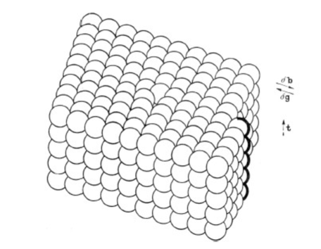
Figure 18.1: Edge dislocation in a simple cubic crystal (Kröner [6]): The dislocation line along an ending half-plane of the crystal is parallel to the vector $\mathbf{t}$. The Burgers vector, $\delta\mathbf{b}$, characterizing the missing half-plane, is perpendicular to $\mathbf{t}$. The vector $\delta\mathbf{g}$ describes the gliding of the dislocation as it enters the ideal crystal.

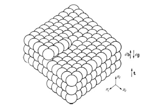
Figure 18.2: Screw dislocation [6]: Here the Burgers vector, $\delta\mathbf{b}$, is parallel to $\mathbf{t}$, the direction of the dislocation line.

We can describe the elastic strain and stress around a crystal dislocation by means of a corresponding Volterra dislocation, provided we use an anisotropic elastic medium appropriate for the crystal structure. At a distance of about five lattice constants from the dislocation line, linear elasticity provides an adequate description of the strain and stress of the crystal.

A dislocation in three dimensions can be defined by a Burgers circuit, see [Reprint 18.2], Eq. (14), or the more detailed discussion in [6], around Eqs. (I.12) and (I.13): the displacement field is added up in going once around the dislocation line. The result is the Burgers vector, $\delta b^{a}$.

18.3 Continuous distribution of dislocations.

In Fig. 18.3 we depicted a 2d view of a cubic crystal. If we apply force stresses, $\sigma_{11}$, it is elongated in $x_{1}$-direction, inter alia, see Fig. 18.4.

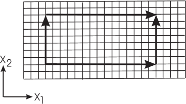
Figure 18.3: The ideal cubic crystal in the undeformed state, see [7]: A “small” parallelogram has been drawn.

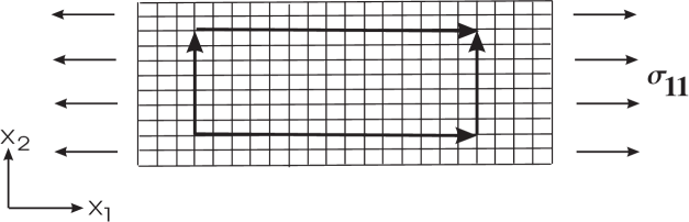
Figure 18.4: Homogeneously strained crystal caused by force stress, $\sigma_{11}$ [7]: The average distances of the lattice points change. The parallelogram remains closed.

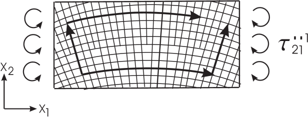
Figure 18.5: Deformation of a cubic crystal by edge dislocations of type $\alpha_{12}{}^{1}$ [7]: The relative orientations of the lattice planes in 2-direction change. A vector in $x_{2}$-direction will rotate, if parallelly displaced along the $x_{1}$-direction. As a consequence, a contortion $K_{112}=-K_{121}$ emerges and the closure failure of the “infinitesimal” parallelogram occurs.

If a sufficient number of dislocations populate a crystal, then a continuum or field theory of dislocations is appropriate. In order to give an idea of such an approach, let us look at a cubic crystal in which several dislocations are present, see Fig. 18.5. By averaging over, we can define a dislocation density tensor, $\alpha_{bc}{}^{a}=-\alpha_{cb}{}^{a}$, with nine independent components:

$$\delta b^{a}=\alpha_{bc}{}^{a}dA^{bc}\,,\qquad\text{with}\qquad dA^{bc}=-dA^{cb}$$ (18.1)

as (2d) area element. In Fig. 18.5 we drew the 12-plane, and the Burgers vector has only the $\delta b^{1}$ component. Thus, in Fig. 18.5, only the $\alpha_{12}{}^{1}=-\alpha_{21}{}^{1}$ components of the dislocation density are nonvanishing. In exterior calculus, we have, quite generally, the dislocation density 2-form $\alpha^{a}=\frac{1}{2}\alpha_{bc}{}^{a}dx^{b}\wedge dx^{c}$.

It can be shown [8] that the crystal in Fig. 18.5 reacts under those conditions with spin moment stresses $\tau_{ab}{}^{c}=-\tau_{ba}{}^{c}$, that is, in order to balance the dislocations, those spin moment stresses have to be applied, as indicated in the figure.

18.4 Kondo’s fundamental identification of dislocation
density with Cartan’s torsion (1952)

In [Reprint 18.1] it is shown that, by using the lattice directions for defining parallel transfer, a “material” connection can be defined that is adapted to the crystal structure. Using this connection, one can define parallel transfer and build up small parallelograms. We depicted this in Fig. 18.3 for the undeformed ideal crystal, in Fig. 18.4 for the crystal deformed by stress and in Fig. 18.5 for the case of the presence of dislocations. We see how the parallelogram is cracked. In this way, as is explained in detail in [Reprint 18.1], the Frank–Burgers circuit for defining dislocations maps to the Cartan circuit defining the torsion.

This fundamental interrelationship was first uncovered by Kondo [9] in 1952. Later, in 1955, the same observation has been made by Bilby, Bullough, and Smith [10]:

… A manifold with a Euclidean metric but asymmetric connexion has many unfamiliar properties. Its geodesics, or curves of shortest length, are the straight lines of ordinary space, but its paths, or autoparallel curves, are not. Further, infinitesimal closed parallelograms do not exist in it (Synge & Schild 1949). It is this last property, of course, which is most intimately connected with the continuously dislocated state. This is very clearly seen by considering models of dislocated states made from wooden balls and flexible curtain wire (Bilby 1950).

Finally, it is an obvious physical requirement that the lattice be uniquely defined everywhere; this means that the manifold must possess the property of distant parallelism …

The result of Kondo and Bilby et al. induced a vast body of literature of mixed quality. We can only refer to a few selected references. From a gravitational point of view, the papers of Katanaev and Volovich [11, 12] should be mentioned for their impact on the understanding of 3d gravity. Ruggiero and Tartaglia [13] had similar thoughts with respect to an interpretation of the 4d EC-theory. Earlier, Kleinert [14] used the dislocation–torsion concept in a theory of melting, inter alia. We mentioned above that the displacement field around a dislocation is double valued, whereas the strain and stress are single-valued. Generalizing this fact, Kleinert [15] developed a theory of multivalued fields and a statistical theory for lattice defect. In some applications he also treats 4d gravity with torsion.

Lazar et al. [16, 17, 18, 19, 20] used the structures of the translational gauge theory of gravity (teleparallelism), see Chapter 6, and developed a 3d field theory of dislocations in quite some detail. Moreover, using gauge ideas, Böhmer and Obukhov [21] proposed a theory for rotational elasticity. In the corresponding elastic body, only spin moment stress is acting, which is proportional to the rotational deformation, $\omega$, of the body; this is a modern incarnation of MacCullagh’s (1837) rotationally elastic aether. The $\omega$ corresponds to the contortion, see Eq. (2.8), of the underlying 3d teleparallel Riemann–Cartan geometry. Finally, we mention an essay [22] on torsion and its application in physics.

Chapter 19     The Yang Episode: A Historical Case Study^∗

Reprinted papers:

• C. N. Yang, Integral formalism for gauge fields, Phys. Rev. Lett. 33, 445–447 (1974).

• C. N. Yang’s 1982 comments on his paper [19.1] in: Chen Ning Yang, Selected Papers 1945–1980, with commentary, 2005 edition (World Scientific, Singapore, 2005) pp. 73–74; extract, p. 74.

• C. N. Yang 1983 quoted in: C. W. F. Everitt, Gravity Probe B: I. The scientific implications, Sixth Marcel Grossmann Meeting on General Relativity, Part B (World Scientific, Singapore, 1992) pp. 1632–1644; extract, pp. 1641–1642.

• C. N. Yang 1986 quoted in: Jong-Ping Hsu, D. Fine (eds.), 100 Years of Gravity and Accelerated Frames, the deepest insights of Einstein and Yang-Mills (World Scientific, Hackensack, NJ, 2005) p. 390.

• W.–T. Ni, Yang’s gravitational field equations, Phys. Rev. Lett. 35, 319–320 (1975).

No doubt, C. N. Yang is an eminent physicist of our day and, as such, a historic personality. Let us turn to his [Reprint 19.1]. In the context of reformulating the local formalism of gauge theories of non-Abelian groups (see Chapter 3) in a global way—he calls it differential versus integral formalism—he comes up, in his Eq. (3), with a new definition of the gauge field (strength), $f_{\mu\nu}{}^{k}$; here $\mu,\nu$ are spacetime indices and $k$ enumerates the generators of the non-Abelian group. He then chooses a spacetime with a Riemannian metric. Subsequently, in Eq. (13), he is able to define a conserved current as a source of $f_{\mu\nu}{}^{k}$ according to $J_{\mu}{}^{\kappa}:=$ $g^{\nu\lambda}f_{\mu\nu\,\,||\lambda}{}^{k}\;\,\,$, where the double stroke denotes the gauge-covariant derivative.

On the Riemannian manifold, Yang defines the parallel displacement by means of the Riemann/Levi-Civita connection. His indices, $\alpha,\beta$, see Eq. (15), can be understood as anholonomic frame indices. As a group transforming the frame, he considers the $GL(n,R)$ (we specialize here on $n=4$ spacetime dimensions). The non-Abelian gauge group of Yang–Mills theory is put in analogy to the $GL(4,R)$ for gravitation. He could have taken $SO(1,3)$, since he has a metric and could define, as Utiyama did (whom he cites), the frames to be orthonormal, but he didn’t. The gravitational field strength is the Riemann tensor, $-R^{\alpha}{}_{\beta\mu\nu}$. The gravitational current would be a $GL(4,R)$-algebra valued vector density (or rather a 3-form) proportional to $-g^{\nu\lambda}R^{\alpha}{}_{\beta\mu\nu;\lambda}$ (the semicolon denotes the Riemannian covariant derivative), that is, the hypermomentum current of Chapter 9. Clearly, Yang is now in trouble: for gravity he needs the energy-momentum current. Hence, for the time being, he puts the source to zero and only comes up with a corresponding vacuum field equation of gravity.

At the time the paper appeared it was anachronistic, since the results of Sciama and Kibble were apparently overlooked. We all can make mistakes. But the mistake of a famous physicist and Nobel prize winner propagates to the most distant corners of the world. This paper, according to the data bank inSPIRE (Stanford-Linear-Accelerator), was cited over 300 times until present day. Again and again people are misled by Yang’s assumption that the $GL(4,R)$ is the gauge group of gravity. It is for this reason that we want to put the paper of Yang and its aftermath in proper perspective.

19.1 Yang’s vacuum field equation of gravity

Yang proposed the following vacuum field equation for gravity (with $R_{\mu\alpha}$ as the Ricci tensor):

$$R_{\mu\alpha;\beta}-R_{\mu\beta;\alpha}=0\,,$$ (19.1)

see [Reprint 19.1], Eq. (19). He assumed that the connection entering the curvature tensor is Riemannian. Then, using the Bianchi identity, Eq. (19.1) can be rewritten in terms of the curvature tensor (in Schouten’s conventions) as

$$R^{\mu\delta}{}_{\alpha\beta;\delta}=0\,.$$ (19.2)

Even though the same equation was proposed earlier by Lichnerowicz (1958), Stephenson (1958) and Kilmister & Newman (1961), this paper by Yang was widely read (and cited) and made alternatives to Einstein’s field equation look more respectable.

Let us consider how Yang’s attitude towards his equation changed over time. In 1982, that is eight years later [Reprint 19.2], he underlined the importance of Eq. (19.1) as a third order partial differential equation (PDE) for the metric. In the subsequent year [Reprint 19.3], he conjectured a symmetry beyond Einstein’s theory should involve spin and rotation, but also the “deep geometrical concept called torsion”. With respect to Eq. (19.1), he stated that this equation should involve spin. Accordingly, Yang was very close to the assumption that the source of his equation should be the spin. But he left it at this somewhat indefinite conjecture. In referring to the Gravity Probe-B experiment [Reprint 19.3], he also spoke of spin; however, it is not clear whether he meant elementary particle spin in the context of his field equation Eq. (19.1) or the orbital angular momenta of the quartz gyros of the experiment.

Eventually, in 1986 [Reprint 19.4], he stressed that besides the field strength of electrodynamics, $F_{\mu\nu}$, the curvature, $R_{\mu\nu}$, is absolutely of primary importance and that in 1974, and apparently also in 1986, he could not write down the right-hand-side of Eq. (19.1). At present, Yang continues, “this problem has not been solved.” This is surprizing considering the fact that at the same institute there was active knowledge available on Riemann–Cartan geometry and torsion, see, for instance, [2].

Summing up: The catchwords that Yang used in the context of a possible generalization of his equation are: 3rd order PDE for the metric; spin; rotation; torsion.

19.2 Poincaré gauge theory and Yang’s vacuum equation

In 1961, Kibble [Reprint 4.2] pointed out that, beyond the linear Hilbert–Einstein term, the gravitational Lagrangian in a PG can depend on curvature and torsion:

We now look for a free Lagrangian $\mathfrak{L}_{0}$ for the new fields. Clearly $\mathfrak{L}_{0}$ must be an invariant density, and if we set

$$\mathfrak{L}_{0}\equiv\mathfrak{H}\,L_{0}\,,$$

then it is easy to see, as in the case of linear transformations, that the invariant $L_{0}$ must be a function only of the covariant quantities $R^{ij}{}_{kl}$ [curvature] and $C^{i}{}_{kl}$ [torsion].

But of course, since Yang suppressed the torsion—see, however, his remark to the contrary in [Reprint 19.3]—he could not solve his problem, and he left Eq. (19.1) without providing a source.

If we turn to the framework of PG in order to understand how Yang’s equation has to be interpreted, we know from Chapter 5 that the two field equations with the sources $\mathfrak{T}_{\alpha}$ (energy-momentum of matter) and $\mathfrak{S}_{\alpha\beta}=-\mathfrak{S}_{\beta\alpha}$ (spin of matter) read (in exterior calculus)

$$DH_{\alpha}-E_{\alpha} = \mathfrak{T}_{\alpha}\,,$$ (19.3)

$$DH_{\alpha\beta}-E_{\alpha\beta} = \mathfrak{S}_{\alpha\beta}\,.$$ (19.4)

If $V$ is the Lagrangian of the gauge field, the gravitational excitations are given by ($T^{\alpha}$ = torsion, $R^{\alpha\beta}$ = curvature) $H_{\alpha}=-{\partial V}/{\partial T^{\alpha}}$ and $H_{\alpha\beta}=-{\partial V}/{\partial R^{\alpha\beta}}$. For the energy-momentum and the spin of gravity we have ($e_{\alpha}$ = frame, $\rfloor$ = interior product, $\wedge$ = exterior product, $\vartheta^{\alpha}$ = coframe)

$$E_{\alpha}=e_{\alpha}\rfloor V+(e_{\alpha}\rfloor T^{\beta})\wedge H_{\beta}+(e_{\alpha}\rfloor R^{\beta\gamma})\wedge H_{\beta\gamma}\qquad\text{and}\qquad E_{\alpha\beta}=-\vartheta_{[\alpha}\wedge H_{\beta]}\,,$$ (19.5)

respectively.

Let us take a Yang–Mills type gravitational toy Lagrangian

$$V=\frac{1}{\varrho}\;{}^{\star}R_{\alpha\beta}\wedge R^{\alpha\beta}\,.$$ (19.6)

Then the field equations read

$${}^{\star}R_{\beta\gamma}\wedge(e_{\alpha}\rfloor R^{\beta\gamma})-R^{\beta\gamma}\wedge(e_{\alpha}\rfloor\,^{\star}R_{\beta\gamma}) = \varrho\,\mathfrak{T}_{\alpha}\,,$$ (19.7)

$$\boxed{D\,^{\star}R_{\alpha\beta}} = \varrho\,\mathfrak{S}_{\alpha\beta}\,.$$ (19.8)

The expression in the box corresponds to the left-hand-side of Yang’s equation Eq. (19.1) or Eq. (19.2), provided one puts the torsion, $T^{\alpha}$, equal to zero. Therefore, the Yang equation can be found from the field equations (19.7) and (19.8) for $T^{\alpha}=0$ in the source-free case $\mathfrak{T}_{\alpha}=0\,,\,\mathfrak{S}_{\alpha\beta}=0$; however, one additionally finds the constraint of vanishing gravitational energy-momentum $E_{\alpha}=0$ or ${}^{\star}R_{\beta\gamma}\wedge(e_{\alpha}\rfloor R^{\beta\gamma})-R^{\beta\gamma}\wedge(e_{\alpha}\rfloor\,^{\star}R_{\beta\gamma})=0$. The would-be source of Yang’s equation turns out to be the spin current 3-form of matter $\mathfrak{S}_{\alpha\beta}$. Accordingly, we found the proper place of Yang’s vacuum equation in the framework of PG in some unphysical limit.

19.3 Exact vacuum solutions of Yang’s equation and
vanishing gravitational energy

Let us follow the discussion of Yang’s paper. Soon after its publication, Pavelle (1975) and Thompson (1975) studied solutions of Eq. (19.1). The clearest and most comprehensive paper is that of Wei-Tou Ni [Reprint 19.5]. He found that Eq. (19.1) encompasses vacuum solutions of Einstein’s equation with cosmological constant as well as those of Nordström’s gravitational theory.

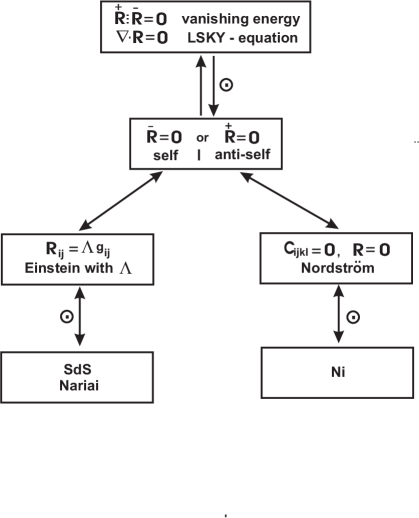
Figure 19.1: Exact spherically symmetric vacuum solutions (denoted by $\odot$) of Yang’s field equation Eq. (19.1) according to [3]: We refer to Eq. (19.1) as LSKY-equation in order to acknowledge the earlier contributions of Lichnerowicz, Stephenson, and Kilmister & Newman. SdS = Schwarzschild–de Sitter solution, Nariai(’s solution), Ni(’s solution).

Later, these types of ideas were worked out by Baekler et al. [3] in the context of PG and, in particular, for vanishing torsion. These authors studied vacuum solutions of Eq. (19.7) and Eq. (19.8) with $T^{\alpha}=0$. They were able to show that Eq. (19.7), in the vacuum case, can be rewritten as a product of the selfdual and the anti-selfdual parts of the curvature, see Fig. 19.1, first line; compare also with Wallner [4] and Obukhov et. al. [5]. The spherically symmetric solutions then split into two branches: One branch where the anti-selfdual part vanishes and another one where the selfdual part of the curvature vanishes. For the spherically symmetric case, this yields either the vacuum solutions of Einstein theory with cosmological constant or that of the Nordström’s theory. Thus, quite an interesting structure arises and we can integrate the results of Pavelle, Thompson, and Ni into a quadratic PG in a degenerate limit.

Still, Yang’s approach led to a dead end and we recognize, as we already did explicitly in Chapters 4 and 5, that neither the $GL(4,R)$ nor the $SO(1,3)$ is the gauge group of gravity, we rather have to turn to the affine groups $A(4,R)=T(4)\;{\hbox to0.0pt{$\supset$\hss}\times}\;GL(4,R)$ or $P(1,3)=T(4)\;{\hbox to0.0pt{$\supset$\hss}\times}\;SO(1,3)$, respectively.

Index

Acceleration

rotational 105

length 105

translational 5

length 5

Action, see Lagrangian

Angular momentum 4, 287

conservation law 4

orbital 4

spin 4

Anti-de Sitter (AdS) gauge theory 382

Cartan geometry 384

Ashtekar variables 108, 238

Asymptotic symmetry of PG in 3d 561

AdS/CFT correspondence 562

asymptotic conditions 561

central charges (classical) 562

Virasoro algebra 561–562

Autoparallel 18, 264, 591

Belinfante–Rosenfeld procedure 318

Bianchi identities 265, 560

first 176, 265

second 265

Black hole with torsion in 3d 560

conserved charges 561

entropy 562

Bonse–Wroblewski experiment 105

Burgers vector 589

Cartan’s spiral staircase 561, 593

Casimir operator 4

Charges, see Currents

Christoffel symbol 6

Classical solutions of PG in 3d

anti-de Sitter solution 561

circularly symmetric 561

with conformally flat metric 561

plane-fronted wave 561

Coframe 17

anholonomic (or arbitrary) 101

holonomic (or natural) 101

normal in metric-affine space 317

orthonormal 20, 103

Colella–Overhauser–Werner experiment 102

Computer algebra 526

Conformal gauge theory (CG) 365

action 368, 369

Connection 19

anti-de Sitter 382

Christoffel symbol 6

Levi-Civita 18

linear (affine) 19

Lorentz 237, 316

propagating 564

metric-compatible 17

post-Riemannian

distortion 20

Riemann–Cartan 286

Riemannian 4, 18, 28, 286

shear part of 316

self-dual 108

symmetric 4, 28

teleparallel 20

Weyl 18

Contortion 20, 560, 590

Cosmological constant 8, 501, 620, 621

effective 501, 527, 560

Cosmological principle 498

in general relativity (GR) 498

Robertson–Walker metric 501

in Riemann–Cartan spacetime 498

Cosserat continuum 21, 103

Cotton 2-form 174, 560

Covariant derivative 285, 288, 367, 384

parallel transport 285

Currents

conservation laws 288

electric charge 22

isospin 71, 72

dynamical 288

Noether 288, 366

scale (dilation) 287, 319, 501

charge 529

shear 319, 501

charge 319, 529

special conformal 367

spin 501

translational 318

Curvature 19, 174

anti-de Sitter (AdS) 383

irreducible decomposition 174

Ricci tensor (1-form) 19, 560

Riemann 6

Riemann–Cartan 178

Weyl 289

Weyl (conformal) 560

Dark energy 499

in Einstein–Cartan theory 499

in metric-affine gravity (MAG) 501

in Poincaré gauge theory (PG)

scalar torsion modes 500

Dirac equation 22, 105, 473

Disclination 588

Dislocation 587

Burgers vector 589, 590

dislocation density 590

2-form 590

dislocation density and torsion 590

edge dislocation 587, 588

screw dislocation 588, 589

Distortion 20

Einstein-Cartan theory (EC)

Ashtekar variables 108

as degenerate PG 177

critical density 107, 108

field equations (Sciama–Kibble) 106

Lagrangian 106

Einstein field equation 8

Einstein laboratory 5, 104

Electromagnetism

excitation 7

field strength 7

Lorentz force 7

Energy-momentum 4, 7, 287, 318

canonical (Noether) 107, 318

conservation law 4

gravitational field 175

metric (Hilbert) 107, 318

Equivalence principle 4

Exact solutions in PG and MAG 525

Baekler–Lee solution 526

Kerr type with torsion 525

with mass, dilation, and shear charges 529

plane-fronted waves in MAG 525, 529

Schwarzschild type with torsion 525, 528

Yilmaz–Rosen metric in PG 530

Flow 3-form 319

Frame

inertial 5

non-inertial 5

normal in metric-affine space 317

Friedmann equation (generalized) 499, 500

Gauge generator, canonical 430

asymptotic condition 430

asymptotic symmetry 430

boundary (surface) term 430, 432

for MAG 433

for PG 433

conserved charge 430

improved 430

Gauge theory 176

compensating field 23, 236, 288

excitation 175

field equations

homogeneous 74

inhomogeneous 74, 75

gauge field strength 382, 617

gauge invariance 288

gauge potential 288

gauge principle 71, 101, 287

of gravity 102

of internal group

Abelian 176

non-Abelian 176

General relativity (GR) 7

field equation 8

Geodesic 6, 18, 591

Goldstone field 383

Gravitational phase shift 618

Gravitational singularities 497, 500

in Einstein–Cartan theory 499

energy condition 498

in MAG 501

in PG 500

of metric 500

of torsion 500

in Weyl gauge theory 501

Gravitational wave 8

Gravity

gravito-electromagnetism 104

gravito-magnetism 104

strong (Yang–Mills type) 179, 526

weak (Newton–Einstein) 179, 525

Group (of transformations)

affine 315

(anti-)de Sitter 381

conformal 365

diffeomorphism 382

Lie 366

non-Abelian 73,

semi-simple 73, 101, 381

simple 365

Lorentz 3, 101, 365

Poincaré 3, 287

representation

linear 367, 368

nonlinear 236, 367, 368, 383

super Poincaré 405

translation 3, 236, 365

Weyl 287

Hamiltonian

of PG 430

Dirac-ADM form 430

Hamiltonian constraints

first class 430

unphysical variables 429

primary 430

if-constraints 430

secondary 430

second class 430

Hamiltonian formalism, covariant 431

Hyperfluid 319, 501

Hypermomentum 319, 472

conservation law 319

intrinsic 319, 472

orbital 319

Inflation, in

Einstein–Cartan theory 499

PG 500

Weyl gauge theory 501

Initial value problem, in

Einstein–Cartan theory 107, 177

PG 176, 177

simple supergravity 407

translation gauge theory 238

Kibble laboratory 102, 104

Killing vector 561

Lagrangian (action), of

(anti-)de Sitter gauge theory 382, 383

conformal gauge theory 368, 369

Einstein–Cartan theory 106

gauge field 174

matter 174

MAG 320

PG 174, 179

translational gauge theory 237

Weyl gauge theory 288, 289

Light deflection 6

Lorentz force 7

Mass

gravitational 4

inertial 4

Matter, classical description of

hyperfluid 319, 501

Weyssenhoff (spin) fluid 470, 498

Lagrangian theory 498

Matter, equations of motion for 469

Matter field

Dirac field 22, 105, 238

Dirac equation 22, 105, 473

Dirac test particle 472

spin precession 473

minimal coupling of 74

Proca field 473

semiclassical approximation 472

with complex phase 473

world-spinor field 320, 473

Maxwell equations 7

Metric 3

metricity condition 286

nonmetricity 18, 262, 286

Robertson–Walker 501

Schwarzschild 289

semi-metric condition 285

Yilmaz–Rosen 530

Metric–affine gauge theory (MAG) 315, 316

action 320

field equations 320

hyperfluid 319

world spinor 320

Metric-affine geometry 20

Minimal coupling 74

Møller’s tetrad theory 236

Multipole formalism 471

covariant conservation laws 470

integrated moments 470

propagation equations 470

single-pole approximation 470, 471

pole-dipole approximation 472

supplementary conditions 471, 472

Noether identities (theorems) 4, 175, 560

Poincaré invariance 174

Nonlinear constraint effects 238, 431

test of viability 431

for PG 431

Nonmetricity 18, 262, 286

Nordström’s theory of gravity 620

Papapetrou–Mathisson equations 471

Pauli–Lubański vector 4

Poincaré gauge theory (PG) xi, 173, 235

excitations 175

total Lagrangian 175

most general quadratic 179

two field equations 175

PG in 3d 559

Bianchi identities 560

Lorentz connection, propagating 564

Noether identities 560

supergravity 563

topological model 560

Chern–Simons formulation 563

Ricci tensor (1-form) 19, 560

Spacetime, geometry of

affine 315, 316

(anti-)de Sitter 381

Finsler 20

metric-affine 20, 286

Minkowski 287

Riemann–Cartan 20, 173, 235

Riemann(ian) 285

teleparallel 20, 235

Weitzenböck 235

Weyl 286

Weyl–Cartan 286

Special relativity 3

Spin of gravitational field 175

Spin moment (torque) stress 21, 590

Spinors

Dirac (4 components) 22

Majorana 406, 407

Pauli (2 components) 22

Stress 21

around a dislocation 589

Superalgebra

Coleman–Mandula theorem 406

generators 406

Majorana spinor 406

Supergravity (SuGra) 405

(anti-)de Sitter 409, 410

auxiliary fields 407

Einstein–Cartan (EC) 406

Majorana vector-spinor (gravitino) 406

Rarita–Schwinger action 406

in 11 dimensions 407

Poincaré 406

with propagating Lorentz connection 408

simple 406

first/second order form 407

teleparallel 408

Super PG, see Supergravity

Symmetry (transformation)

conformal 288

special conformal 365

dilatation 287, 288

dilation 288

local (or gauge) 23, 286

Poincaré 4, 287

translation 3, 236, 365

Lorentz transformation 3, 101, 365

rigid (or global) 4, 287

scale 286, 287, 365

spontaneously broken 289, 383

supersymmetry (SS) 405

Weyl 288

Teleparallel theory 235

teleparallel equivalent of GR (GR_||) 237

geometry (distant parallelism) 20, 591

Test body, the motion of 470

in MAG 472

with microstructure

intrinsic spin 471

intrinsic hypermomentum 472

without microstructure 472

in PG 470

Tetrad 236, 367, 368, 382

Torsion 18, 19, 173, 237, 261, 262, 263, 382

contortion 20, 560, 590

cracked parallelogram 263, 590

in dislocation theory 587

and electromagnetism 267

and Gravity Probe B 266

irreducible decomposition 173

singularities 180, 500

in string theory 267

Translation gauge theory (TG) 178, 235, 266

as degenerate PG 177

field equations 178, 236

Lagrangian 237

time evolution of torsion 238

Variation

of metric, coframe, connection 348, 353

mixed variation 23

Weyl covector (1-form) 18, 285

Weyl(–Cartan) gauge theory 285, 287

dilaton 289

Lagrangian 289

low energy limit 289

“Weyl charge” 528

World spinor 320, 473

Yang–Mills theory

field equation 75

Yang’s field equation of gravity 617, 618, 620

exact solutions, of

Thompson,  Pavelle,  Ni  620

LSKY-equation 621

References

- [1] J. P. Hsu and D. Fine (eds.), 100 Years of Gravity and Accelerated Frames. The deepest insights of Einstein and Yang–Mills (World Scientific, Singapore, 2005).
- [2] H. A. Lorentz et al., The Principle of Relativity, translated by W. Perrett and G. B. Jeffery (Dover, New York, 1952).
- [3] Y. Kosmann-Schwarzbach, The Noether Theorems (Springer, New York, 2011).
- [4] W.-K. Tung, Group Theory in Physics (World Scientific, Singapore, 1985).
- [5] E. Wigner, On unitary representations of the inhomogeneous Lorentz group, Annals of Mathematics 40, 149–204 (1939); see also K. Huang, Quarks, Leptons & Gauge Fields, 2nd ed. (World Scientific, Singapore, 1992).
- [6] H. Minkowski, Space and time, in: [2], pp. 73–91.
- [7] H. Minkowski, Die Grundgleichungen für die elektromagnetischen Vorgänge in bewegten Körpern, Königliche Gesellschaft der Wissenschaften zu Göttingen, Mathematisch-Physikalische Klasse, Nachrichten, pp. 53–111 (1908).
- [8] A. Einstein, Über das Relativitätsprinzip und die aus demselben gezogenen Folgerungen, Jahrbuch der Radioaktivität und Elektronik 4, 411–462 (1907/8); Erratum 5, 98–99 (1908).
- [9] E. Fischbach and C. L. Talmadge, The Search for Non-Newtonian Gravity (Springer, New York, 1999).
- [10] A. Einstein, The Meaning of Relativity, 5th ed. (Princeton University Press, Princeton, 1955) [first published in 1922].
- [11] B. Mashhoon, Nonlocal special relativity, Ann. Phys. (Berlin) 17, 705–727 (2008) [arXiv:0805.2926].
- [12] E. L. Schucking, Gravitation is torsion, arXiv:0803.4128. E. L. Schucking and E. J. Surowitz, Einstein’s apple: his first principle of equivalence, arXiv:gr-qc/0703149.
- [13] H. Weyl, Space-Time-Matter, translated from the fourth German edition of 1921 by H. Brose (Dover, New York, 1952).
- [14] J. Ehlers, F. A. E. Pirani, and A. Schild, The geometry of free fall and light propagation, in: L. O’Raifeartaigh (ed.), General Relativity, papers in honour of J. L. Synge (Clarendon Press, Oxford 1972), pp. 63–84.
- [15] J. Audretsch, F. Gähler, and N. Straumann, Wave fields in Weyl spaces and conditions for the existence of a preferred pseudoriemannian structure, Commun. Math. Phys. 95, 41–51 (1984).
- [16] J. Audretsch, F. W. Hehl, and C. Lämmerzahl, Matter wave interferometry and why quantum objects are fundamental for establishing a gravitational theory, Proceeding of the Bad Honnef School on Gravitation, Lecture Notes in Physics 440, 368–407 (1992).
- [17] R. Adler, M. Bazin, and M. Schiffer, Introduction to General Relativity, 2nd ed. (McGraw-Hill, New York, 1975).
- [18] A. Einstein, Eine neue formale Deutung der Maxwellschen Feldgleichungen der Elektrodynamik (A new formal interpretation of Maxwell’s field equations of electrodynamics), Sitzungsber. Königl. Preuss. Akad. Wiss. Berlin 184–188 (1916); see also A.J. Kox et al. (eds.), The Collected Papers of Albert Einstein Vol. 6 (Princeton University Press, Princeton, 1996) pp. 263–269.
- [19] J. A. Schouten, Tensor Analysis for Physicists, 2nd ed., reprinted (Dover: Mineola, New York, 1989).
- [20] E. J. Post, Formal Structure of Electromagnetics – General covariance and electromagnetics (North Holland, Amsterdam, 1962; and Dover, Mineola, New York, 1997).
- [21] F. W. Hehl, Maxwell’s equations in Minkowski’s world: their premetric generalization and the electromagnetic energy-momentum tensor, Ann. Phys. (Berlin) 17, 691–704 (2008) [arXiv:0807.4249].
- [22] F. W. Hehl and Yu. N. Obukhov, Foundations of Classical Electrodynamics – Charge, flux, and metric (Birkhäuser, Boston, MA, 2003).
- [23] A. Einstein, Kosmologische Betrachtungen zur allgemeinen Relativitätstheorie (Cosmological considerations of the general theory of relativity), Sitzungsber. Königl. Preuss. Akad. Wiss. Berlin 142–152 (1917); see also A.J. Kox et al. (eds.), The Collected Papers of Albert Einstein Vol. 6 (Princeton University Press: Princeton, 1996) pp. 540–552.

References

- [1] G. Hessenberg, Vektorielle Begründung der Differentialgeometrie, Mathematische Annalen 78, 187–217 (1917).
- [2] E. L. Schücking, Einstein’s apple and relativity’s gravitational field, arXiv:0903.3768v2.
- [3] K. Reich, Die Entwicklung des Tensorkalküls, Vom absoluten Differentialkalkül zur Relativitätstheorie (Birkhäuser, Basel, 1994).
- [4] T. Levi-Civita, Nozione di parallelismo in una varietà qualunque, Rend. Circ. Mat. Palermo 42, 173–205 (1917); T. Levi-Civita, The Absolute Differential Calculus (calculus of tensors), translated by M. Long, edited by E. Persico (Blackie, Glasgow, 1926).
- [5] H. Weyl, Gravitation und Elektrizität, Sitzungsber. Preuss. Akad. Wiss. 465–480 (1918); Eine neue Erweiterung der Relativitätstheorie, Annalen der Physik IV. 59 [or 364], 101–133 (1917).
- [6] J. A. Schouten, Die direkte Analysis zur neueren Relativitätstheorie, Verh. Kon. Akad. Amsterdam 12 (no.6) 95 pages (1918/19).
- [7] A. S. Eddington, A generalisation of Weyl’s theory of the electromagnetic and gravitational fields, Proc. Roy. Soc. London A 99, 104–122 (1921).
- [8] É. Cartan, On Manifolds with an Affine Connection and the Theory of General Relativity, translation by A. Magnon and A. Ashtekar of the French original of 1923/24, with a foreword of A. Trautman (Bibliopolis, Naples, 1986).
- [9] A. Einstein, Preface (dated 04 April 1955), in: M. Pantaleo (ed.), Cinquant’ anni di Relatività 1905–1955 (Edizioni Giuntine and Sansoni Editore, Florence, 1955) (translation by F. Gronwald, D. Hartley, and F.W. Hehl).
- [10] J. A. Schouten, Ricci Calculus, 2nd ed. (Springer, Berlin, 1954).
- [11] F. W. Hehl, J. D. McCrea, E. W. Mielke, and Y. Ne’eman, Metric affine gauge theory of gravity: Field equations, Noether identities, world spinors, and breaking of dilation invariance, Phys. Rept. 258, 1–171 (1995).
- [12] R. Weitzenböck, Invariantentheorie (Noordhoff, Groningen, 1923).
- [13] R. Weitzenböck, Differentialinvarianten in der Einsteinschen Theorie des Fernparallelismus, Sitzungsber. Preuss. Akad. Wiss. Berlin, Phys.-math. Klasse 466–474 (1928).
- [14] R. Debever (ed.), Elie Cartan–Albert Einstein, Lettres sur le Parallélisme Absolu 1929–1932 (Académie Royale de Belgique, Brussels, and Princeton University Press, Princeton, NJ, 1979).
- [15] E. Cartan, Notice historique sur la notion de parallélisme absolu, Mathematische Annalen 102, 698–706 (1930).
- [16] A. Einstein, Riemann-Geometrie mit Aufrechterhaltung des Begriffes des Fernparallelimus Sitzungsber. Preuss. Akad. Wiss. Berlin, Phys.-math. Klasse 217–221 (1928); A. Einstein, Neue Möglichkeit für eine einheitliche Feldtheorie von Gravitation und Elektrizität, ibid. 224–227 (1928); A. Einstein, Zur Einheitlichen Feldtheorie, ibid. 2–7 (1929).
- [17] A. Einstein, Auf die Riemann-Metrik und den Fern-Parallelismus gegründete einheitliche Feldtheorie, Mathematische Annalen 102, 685–697 (1930).
- [18] T. Sauer, Field equations in teleparallel spacetime: Einstein’s fernparallelismus approach towards unified field theory, Historia Math. 33, 399–439 (2006) [arXiv:physics/0405142].
- [19] H. E. Salzer, Two letters from Einstein concerning his distant parallelism field theory, Archive for History of Exact Sciences 12, 89–96 (1974).
- [20] C. Møller, Conservation laws and absolute parallelism in general relativity, Mat.-Fys. Skr. Dan. Vidensk. Selsk. 1, no. 10 (1961).
- [21] C. Pellegrini and J. Plebański, Tetrad fields and gravitational fields, Mat.-Fys. Skr. Dan. Vidensk. Selsk. 2, no. 4 (1963).
- [22] E. Schrödinger, Space-Time Structure (Cambridge University Press, Cambridge, 1960).
- [23] A. Einstein, The Meaning of Relativity, 5th ed. (Princeton University Press, Princeton, NJ, 1955).
- [24] H. Rund, The Differential Geometry of Finsler Spaces (Springer, Berlin, 1959).
- [25] G. S. Asanov, Finsler Geometry, Relativity and Gauge Theories (Reidel Publishing, Dordrecht, 1985).
- [26] G. Yu. Bogoslovsky, A viable model of locally anisotropic space-time and the Finslerian generalization of the relativity theory, Fortschritte der Physik 42, 143–193 (1994).
- [27] V. Perlick, Fermat principle in Finsler spacetimes, Gen. Rel. Grav. 38, 365–380 (2006) [arXiv:gr-qc/0508029].
- [28] H. F. M. Goenner, On the history of geometrization of space-time: from Minkowski to Finsler geometry, arXiv:0811.4529.
- [29] C. Lämmerzahl, D. Lorek, and H. Dittus, Confronting Finsler space-time with experiment, Gen. Rel. Grav. 41, 1345–1353 (2009) [arXiv:0811.0282].
- [30] E. Cosserat and F. Cosserat, Théorie des corps déformables, (Hermann, Paris, 1909); translated into English by D. Delphenich, email: daviddelphenich@yahoo.com (2007).
- [31] E. Kröner, Continuum theory of defects, in: R.Balian et al. (eds.), Physics of Defects, Les Houches, Session XXXV, 1980 (North-Holland, Amsterdam, 1981) p. 215.
- [32] L. O’Raifeartaigh, The Dawning of Gauge Theory (Princeton University Press, Princeton, NJ, 1997).
- [33] L. B. Okun, V A Fock and gauge symmetry, Physics Uspekhi 53, 835–837 (2010).
- [34] V. Fock and D. Iwanenko, Über eine mögliche Deutung der relativistischen Quantentheorie, Z. Physik 54, 798–802 (1929).
- [35] V. Fock, Geometrisierung der Diracschen Theorie des Elektrons, Z. Physik 57, 261–277 (1929).
- [36] F. Gronwald and F. W. Hehl, On the gauge aspects of gravity, in: P.G. Bergmann et al. (eds.), Proc. Int. School of Cosm. & Gravit. 14th Course: Quantum Gravity. Held in Erice, Italy. Proceedings (World Scientific, Singapore, 1996) pp. 148–198 [arXiv:gr-qc/0601013].
- [37] A. Einstein, Einheitliche Feldtheorie von Gravitation und Elektrizität, Sitzungsber. Preuss. Akad. Wiss. Berlin 414–419 (1925). Compare: M. Ferraris, M. Francaviglia, and C. Reina, Variational formulation of general relativity from 1915 to 1925, “Palatini’s method” discovered by Einstein in 1925, General Relativity and Gravitation 14, 243–254 (1982).

References

- [1] P. A. M. Dirac, The quantum theory of the electron, Proc. Roy. Soc. Lond. A 117, 610–624 (1928).
- [2] W. Heisenberg, On the constitution of atomic nuclei. I (in German: Über den Bau der Atomkerne. I), Zeitschrift für Physik 77, 1–11 (1932); Part II: 78, 156–164 (1932); Part III: 80, 587–596 (1933).
- [3] E. Wigner, On the consequences of the symmetry of the nuclear Hamiltonian on the spectroscopy of nuclei, Phys. Rev. 51, 106–119 (1937).
- [4] G. Rasche, On the history of the notion “isospin” (in German: Zur Geschichte des Begriffes “Isospin”), Archive for History of Exact Sciences 7, 257–276 (1971).
- [5] N. Kemmer, Field theory of nuclear interaction, Phys. Rev. 52, 906–910 (1937); N. Kemmer, The charge-dependence of nuclear forces, Proc. Cambr. Phil. Soc. 34, 354–364 (1938).
- [6] R. Mills, Gauge fields, Am. J. Phys. 57, 493–507 (1989).
- [7] F. Gronwald and F. W. Hehl, On the gauge aspects of gravity, in: P.G. Bergmann et al. (eds.), Proc. Int. School of Cosm. & Gravit. 14th Course: Quantum Gravity. Held in Erice, Italy. Proceedings (World Scientific, Singapore, 1996) pp. 148–198 [arXiv:gr-qc/9602013].
- [8] L. O’Raifeartaigh, The Dawning of Gauge Theory (Princeton University Press, Princeton, NJ, 1997).
- [9] L. O’Raifeartaigh, Hidden gauge symmetry, Rep. Progr. Phys. 42, 159–223 (1979).
- [10] L. O’Raifeartaigh, Group Structure of Gauge Theories (Cambridge University Press, Cambridge, 1986).
- [11] P. H. Frampton, Gauge Field Theories, 3rd edition (Wiley-VCH, Weinheim, 2008), Chapter 1.
- [12] A. O. Barut and R. Raçzka, Theory of Group Representations and Applications (PWN—Polish Scientific, Warsaw, 1977), Chapter 1.
- [13] J. J. Sakurai, Theory of strong interactions, Ann. Phys. (N.Y.) 11, 1–48 (1960).
- [14] R. Mills, Model of confinement for gauge theories, Phys. Rev. Lett. 43, 549–551 (1979).

References

- [1] R. Colella, A.W. Overhauser, and S. A. Werner, Observation of gravitationally induced quantum interference, Phys. Rev. Lett. 34, 1472–1474 (1975); H. Rauch and S. A. Werner, Neutron Interferometry: Lessons in Experimental Quantum Mechanics (Oxford University Press, Oxford, 2000).
- [2] Yu. A. Alexandrov, Fundamental Properties of the Neutron, translated by T. F. Drozdova (Clarendon Press, Oxford, 1992).
- [3] V. V. Nesvizhevsky, H. G. Börner, A. K. Petukhov, H. Abele, S. Baessler et al., Quantum states of neutrons in the Earth’s gravitational field, Nature 415, 297–299 (2002).
- [4] S. Baessler, A. Gagarski, L. Grigorieva, M. Kreuz, F. Naraghi et al., The GRANIT project: Status and Perspectives, arXiv:1202.2784 [5 pages].
- [5] M. Kasevich and S. Chu, Atomic interferometry using stimulated Raman transitions, Phys. Rev. Lett. 67, 181–184 (1991); A. D. Cronin, J. Schmiedmayer, and D. E. Pritchard, Optics and interferometry with atoms and molecules, Rev. Mod. Phys. 81, 1051–1129 (2009).
- [6] C. G. de Oliveira and J. Tiomno, Representations of Dirac equation in general relativity, Nuovo Cim. 24, 672–687 (1962).
- [7] E. Fischbach, B. S. Freeman, and W.-K. Cheng, General-relativistic hydrogenic systems, Phys. Rev. D 23, 2157–2180 (1981).
- [8] F. W. Hehl, J. Lemke, and E. W. Mielke, Two lectures on fermions and gravity, in: J. Debrus and A. C. Hirshfeld (eds.), Geometry and Theoretical Physics, Proc. of the Bad Honnef School 12–16 Feb. 1990 (Springer, Heidelberg, 1991) pp. 56–140.
- [9] C. Kiefer and C. Weber, On the interaction of mesoscopic quantum systems with gravity, Ann. Physik (Berlin) 14, 253–278 (2005) [arXiv:gr-qc/0408010].
- [10] Yu. N. Obukhov, A. J. Silenko, and O. V. Teryaev, Dirac fermions in strong gravitational fields, Phys. Rev. D 84, 024025 (2011) [10 pages] [arXiv:1106.0173].
- [11] F. W. Hehl and Yu. N. Obukhov, Élie Cartan’s torsion in geometry and in field theory, an essay. Annales de la Fondation Louis de Broglie 32, 157–194 (2007) [arXiv:0711.1535].
- [12] B. Mashhoon, Gravitoelectromagnetism, in: J. F. Pascual-Sanchez et al. (eds.), Reference Frames and Gravitomagnetism (World Scientific, Singapore, 2001) pp. 121–132 [arXiv:gr-qc/0011014].
- [13] B. Mashhoon, Gravitoelectromagnetism: A Brief review, in: L. Iorio (ed.), The Measurement of Gravitomagnetism: A Challenging Enterprise (NOVA Science, Hauppage, NY, 2007) Chapter 3 [arXiv:gr-qc/031103].
- [14] F. Gronwald and F. W. Hehl, On the gauge aspects of gravity, in: P. G. Bergmann et al. (eds.), Proc. of the 14th Course of the International School of Cosmology and Gravitation on Quantum Gravity, held in Erice, Italy, May 1995 (World Scientific, Singapore, 1996) pp. 148–199 [arXiv:gr-qc/9602013].
- [15] U. Bonse and T. Wroblewski, Measurement of neutron quantum interference, Phys. Rev. Lett. 51, 1401–1404 (1983).
- [16] B. Mashhoon, Neutron interferometry in a rotating frame of reference, Phys. Rev. Lett. 61, 2639–2642 (1988).
- [17] F. W. Hehl and W.-T. Ni, Inertial effects of a Dirac particle, Phys. Rev. D 42, 2045–2048 (1990).
- [18] F. W. Hehl, P. von der Heyde, G. D. Kerlick, and J. M. Nester, General relativity with spin and torsion: Foundations and prospects, Rev. Mod. Phys. 48, 393–416 (1976); see also F. W. Hehl, Four lectures in Poincaré gauge field theory, in: P. G. Bergmann and V. de Sabbata (eds.), Proc. of the 6th Course of the International School of Cosmology and Gravitation on Spin, Torsion, Rotation, and Supergravity, held in Erice, Italy, May 1979 (Plenum, New York, 1980) pp. 5–61 [see http://www.thp.uni-koeln.de/gravitation/mitarbeiter/Erice1979.pdf ].
- [19] F. W. Hehl, J. D. McCrea, E. W. Mielke and Y. Ne’eman, Metric-affine gauge theory of gravity: Field equations, Noether identities, world spinors, and breaking of dilation invariance, Phys. Rept. 258, 1–171 (1995).
- [20] M. Blagojević, Gravitation and Gauge Symmetries (IoP Publishing, Bristol, 2002).
- [21] F. W. Hehl and Yu. N. Obukhov, Foundations of Classical Electrodynamic: Charge, flux, and metric (Birkhäuser, Boston, Massachusetts, 2003).
- [22] I. M. Benn, T. Dereli, and R. W. Tucker, Gauge field interactions in spaces with arbitrary torsion, Phys. Lett. B 96, 100–104 (1980).
- [23] R. A. Puntigam, C. Lämmerzahl, and F. W. Hehl, Maxwell’s theory on a post-Riemannian space-time and the equivalence principle, Class. Quant. Grav. 14, 1347–1356 (1997) [arXiv:gr-qc/9607023].
- [24] Y. Choquet-Bruhat, Spin 1/2 fields in arbitrary dimensions and the Einstein-Cartan theory, in: W. Rindler and A. Trautman (eds.), Gravitation and Geometry, a volume in honour of I. Robinson (Bibliopolis, Naples, 1987) pp. 83–106.
- [25] Y. Choquet-Bruhat, Einstein-Cartan theory with spin 3/2 source and classical supergravity, in: Y. Choquet-Bruhat and T. M. Karade (eds.), Proc. of the Sir Arthur Eddington Centenary Symposium, Vol. 2, On Relativity Theory (World Scientific, Singapore, 1985) pp. 27–56.
- [26] D. D. Bleecker, A new view of the ECSK theory with a Dirac spinor, Gen. Rel. Grav. 22, 299–347 (1990).
- [27] P. Galison, How Experiments End (University of Chicago Press, Chicago, Illinois, 1987).
- [28] V. Ya. Frenkel’, On the history of the Einstein–de Haas effect, Sov. Phys. Uspekhi 22, 580–587 (1979) [Usp. Fiz. Nauk 128, 545–557 (1979)].
- [29] R. F. O’Connell, Contact interactions in the Einstein and Einstein–Cartan–Sciama–Kibble (ECSK) theories of gravitation, Phys. Rev. Lett. 37, 1653–1655 (1976) and erratum 38, 298 (1977).
- [30] R. F. O’Connell, Attractive spin spin contact interactions in the ECSK torsion theory of gravitation, Phys. Rev. D 16, 1247 (1977).
- [31] R. F. O’Connell, Rotation and Spin in Physics, in: I. Ciufolini and R. A. Matzner (eds.), General Relativity and John Archibald Wheeler (Springer, Dordrecht, 2010) pp. 325–336 [arXiv:1009.4401].
- [32] A. Ashtekar, Lectures on Non-perturbative Canonical Gravity (World Scientific, Singapore, 1991).
- [33] C. Kiefer, Quantum Gravity, 3rd ed. (Oxford University Press, Oxford, 2012).
- [34] C. Rovelli, Quantum Gravity (Cambridge University Press, Cambridge, 2004).
- [35] A. Ashtekar, J. D. Romano, and R. S. Tate, New variables for gravity: inclusion of matter, Phys. Rev. D 40, 2572–2587 (1989).
- [36] A. A. Tseytlin, On the first order formalism in quantum gravity, J. Phys. A 15, L105–L110 (1982); see also G. T. Horowitz, Topology change in classical and quantum gravity, Class. Quant. Grav. 8, 587–601 (1991).
- [37] E. W. Mielke, Ashtekar’s complex variables in general relativity and its teleparallelism equivalent, Ann. Phys. (NY) 219, 78–108 (1992).
- [38] M. Bojowald and R. Das, Canonical gravity with fermions, Phys. Rev. D 78, 064009 (2008) [arXiv:0710.5722].
- [39] T. Schücker, Ashtekar’s variables without spin, arXiv:0906.4918 [6 pages].
- [40] P. Baekler and F. W. Hehl, Beyond Einstein-Cartan gravity: Quadratic torsion and curvature invariants with even and odd parity including all boundary terms, Class. Quantum Grav. 28, 215017 (2011) [arXiv:1105.3504].

References

- [1] D. Hartley, Normal frames for non-Riemannian connections, Class. Quantum Grav. 12, L103–L105 (1995).
- [2] B. Z. Iliev, Normal frames and the validity of the equivalence principle: I. Cases in a neighborhood and at a point, J. Phys. A 29, 6895–6902 (1996).
- [3] J. M. Nester, Normal frames for general connections, Ann. Phys. (Berlin) 19, 45–52 (2010).
- [4] J. F. T. Giglio and W. A. Rodrigues, Jr, Locally inertial reference frames in Lorentzian and Riemann-Cartan spacetimes, Ann. Phys. (Berlin) 524, 302–310 (2012) [arXiv:1111.2206].
- [5] F. W. Hehl, J. D. McCrea, E. W. Mielke, and Y. Ne’eman, Metric affine gauge theory of gravity: Field equations, Noether identities, world spinors, and breaking of dilation invariance, Phys. Rept. 258, 1–171 (1995).
- [6] A.A. García, F.W. Hehl, C. Heinicke, and A. Macías, Exact vacuum solution of a (1+2)-dimensional Poincaré gauge theory: BTZ solution with torsion, Phys. Rev. D 67 (2003) 124016 [7 pages] [arXiv:gr-qc/0302097].
- [7] E. Kröner, Continuum theory of defects, in: R. Balian et al. (eds.), Physics of Defects, Les Houches, Session XXXV, 1980 (North-Holland, Amsterdam, 1981) pp. 215–315.
- [8] F. W. Hehl, Four lectures on Poincaré gauge theory, in: P. G. Bergmann and V. de Sabbata (eds.), Cosmology and Gravitation: Spin, Torsion, Rotation and Supergravity (Plenum, New York, 1980) pp. 5–61; see http://www.thp.uni-koeln.de/gravitation/mitarbeiter/Erice1979.pdf.
- [9] H.-J. Blome, C. Chicone, F. W. Hehl, and B. Mashhoon, Nonlocal Modification of Newtonian Gravity, Phys. Rev. D 81, 065020 (2010) [11 pages] [arXiv:1002.1425].
- [10] A. Dimakis, The initial value problem of Poincaré gauge theory in vacuum, I. Second order formalism, II. First order formalism, Ann. Inst. Henri Poincaré A 51, 371–388, 389–417 (1989).
- [11] S. M. Carroll and G. B. Field, Consequences of propagating torsion in connection-dynamic theories of gravity, Phys. Rev. D 50, 3867–3873 (1994).
- [12] Yu. N. Obukhov, V. N. Ponomarev, and V. V. Zhytnikov, Quadratic Poincaré gauge theory of gravity: a comparison with the general relativity theory, Gen. Rel. Grav. 21, 1107–1142 (1989).
- [13] D. Diakonov, A. G. Tumanov, and A. A. Vladimirov, Low-energy general relativity with torsion: A systematic derivative expansion, Phys. Rev. D 84, 124042 (2011) [16 pages] [arXiv:1104.2432].
- [14] P. Baekler and F. W. Hehl, Beyond Einstein-Cartan gravity: Quadratic torsion and curvature invariants with even and odd parity including all boundary terms, Class. Quantum Grav. 28, 215017 (2011) [11 pages] [arXiv:1105.3504].
- [15] R. Hojman, C. Mukku, and W. A. Sayed, Parity violation in metric torsion theories of gravitation, Phys. Rev. D 22, 1915–1921 (1980).
-
[16]
M. Blagojević and I. A. Nikolić, Hamiltonian dynamics
of Poincaré gauge theory: General structure in the time gauge,
Phys. Rev. D 28,
2455–2463 (1983);
I. A. Nikolić, Dirac Hamiltonian structure of Poincaré gauge theory of gravity without gauge fixing, Phys. Rev. D 30, 2508–2520 (1984). - [17] H. J. Yo and J. M. Nester, Hamiltonian analysis of Poincaré gauge theory scalar modes, Int. J. Mod. Phys. D 8, 459–479 (1999) [arXiv:gr-qc/9902032]; H. J. Yo and J. M. Nester, Hamiltonian analysis of Poincaré gauge theory: Higher spin modes, Int. J. Mod. Phys. D 11, 747–779 (2002) [arXiv:gr-qc/0112030]; H. J. Yo and J. M. Nester, Dynamic scalar torsion and an oscillating universe, Mod. Phys. Lett. A 22, 2057–2069 (2007) [arXiv:astro-ph/0612738].
- [18] K. F. Shie, J. M. Nester, and H. J. Yo, Cosmology and the accelerating universe, Phys. Rev. D 78, 023522 (2008) [16 pages] [arXiv:0805.3834].
- [19] X.-z. Li, C.-b. Sun, and P. Xi, Torsion cosmological dynamics, Phys. Rev. D 79, 027301 (2009) [4 pages] [arXiv:0903.3088]; X.-z. Li, C.-b. Sun, and P. Xi, Statefinder diagnostic in a torsion cosmology, JCAP 0904, 015 (2009) [18 pages] [arXiv:0903.4724].
- [20] X.-c. Ao, X.-z. Li, and P. Xi, Analytical approach of late-time evolution in a torsion cosmology, Phys. Lett. B 694, 186–190 (2010) [arXiv:1010.4117].
- [21] M. Adak, Non-minimally coupled Dirac equation with torsion: Poincaré gauge theory of gravity with even and odd parity terms, Class. Quantum Grav. 29, 095006 (2012) [5 pages] [arXiv:1107.0569].
- [22] H.-J. Borchers, Translation Group and Particle Representations in Quantum Field Theory, Lecture Notes in Physics, monograph # 40 (Springer, Berlin, 1996).
- [23] Yu. N. Obukhov, Poincaré gauge gravity: selected topics, Int. J. Geom. Meth. Mod. Phys. 3, 95–138 (2006).
- [24] M. Blagojević, Gravitation and Gauge Symmetries (IOP Publishing, Bristol, 2002); M. Blagojević, Three lectures on Poincaré gauge theory, SFIN A 1, 147–172 (2003) [arXiv:gr-qc/0302040].
- [25] F. W. Hehl, P. von der Heyde, G. D. Kerlick, and J. M. Nester, General relativity with spin and torsion: foundations and prospects, Rev. Mod. Phys. 48, 393–416 (1976).
- [26] A. Trautman, Fiber bundles, gauge fields, and gravitation, in: A. Held (ed.), General Relativity and Gravitation—One Hundred Years after the Birth of Albert Einstein, vol. 1 (Plenum, New York, 1980) pp. 287–308.
- [27] See references in Chapters 10 and 11; T. Kawai, A gauge theory of gravity, Gen. Rel. Grav. 18, 995–1018 (1986); G. Sardanashvily and O. Zakharov, Gauge Gravitation Theory (World Scientific, Singapore, 1992); Y. Ne’eman, Gauge theories of gravity, Acta Phys. Polon. B 29, 827–843 (1998); G. Sardanashvily, On the geometric foundation of classical gauge gravitation theory, arXiv:gr-qc/0201074 [47 pages]; J. Zanelli, Lecture notes on Chern-Simons (super-)gravities, arXiv:hep-th/0502193 [82 pages].
- [28] W. Kopczyński, An anisotropic universe with torsion, Phys. Lett. A 43, 63–64 (1973); A. Trautman, Spin and torsion may avert gravitational singularities, Nature phys. Sci. 242, 7–8 (1973); J. M. Stewart and P. Hájíček, Can spin avert singularities? Nature phys. Sci. 244, 96 (1973); G. D. Kerlick, Cosmology and particle pair production via gravitational spin-spin interaction in the Einstein–Cartan–Sciama–Kibble theory of gravity, Phys. Rev. D 12, 3004–3006 (1975); J. M. Charap and I. Bloomer, Spin, torsion and the singularity theorems of general relativity, Dubna JNR, JINR-E2-10178 (1976), pdf-file available via inSpire; A. Inomata, Effect of the selfinduced torsion of the Dirac sources on gravitational singularities, Phys. Rev. D 18, 3552–3556 (1978).
- [29] J. M. Nester and J. Isenberg, Torsion singularities, Phys. Rev. D 15, 2078–2087 (1977).
- [30] G. Esposito, The singularity problem for space-times with torsion, Nuovo Cim. B 105, 75–90 (1990) and Erratum, B 106, 1315 (1991) [arXiv:gr-qc/9509004]; G. Esposito, Quantum Gravity, Quantum Cosmology and Lorentzian Geometries, Lecture Notes in Physics 12 (Springer, Berlin, 1992); C. M. Zhang, F. P. Chen, and L. C. Garcia de Andrade, Torsion singularity in Weitzenböck space-time, Nuovo Cim. B 110, 231–236 (1995); L. Mullick and P. Bandyopadhyay, Quantum gravity, torsion and space-time singularity, Nuovo Cim. B 113, 1083–1089 (1998).

References

- [1] H. E. Salzer, Two letters from Einstein concerning his distant parallelism field theory, Archive for History of Exact Sciences 12, 89–96 (1974).
- [2] T. Sauer, Field equations in teleparallel spacetime: Einstein’s Fernparallelismus approach towards unified field theory, Historia Math. 33, 399–439 (2006) [arXiv:physics/0405142v1].
- [3] M. Blagojević, Gravitation and Gauge Symmetries (IoP Publishing, Bristol, 2002).
- [4] T. Ortín, Gravity and Strings (Cambridge University Press, Cambridge, 2004).
- [5] H. Meyer, Møller’s tetrad theory of gravitation as a special case of Poincaré gauge theory—a coincidence? Gen. Rel. Grav. 14, 531–547 (1982).
- [6] Y. Itin, Coframe teleparallel models of gravity. Exact solutions, Int. J. Mod. Phys. D 10, 547–573 (2001).
- [7] K. Hayashi and T. Nakano, Extended translation invariance and associated gauge fields, Prog. Theor. Phys. 38, 491–507 (1967).
- [8] Y. Ne’eman, Gravity is the gauge theory of the parallel transport modification of the Poincaré group, in: A. Dold and B. Eckmann (eds.), Lecture Notes in Mathematics 676 (Springer, Berlin, 1978), pp. 189–215.
- [9] A. Trautman, Fiber bundles, gauge fields, and gravitation, in: A. Held (ed.), General Relativity and Gravitation—One Hundred Years after the Birth of Albert Einstein, vol. 1 (Plenum, New York, 1980), pp. 287–308.
- [10] T. Dass, Gauge fields, space-time geometry and gravity, Pramana 23, 433–443 (1984).
- [11] Y. M. Cho, Einstein Lagrangian as the translational Yang–Mills Lagrangian, Phys. Rev. D 14, 2521–2525 (1976).
- [12] J. Julve, A. López-Pinto, A. Tiemblo, and R. Tresguerres, Nonlinear realizations of spacetime symmetries including translations, Gen. Rel. Grav. 28, 759–768 (1996); R. Tresguerres and E. W. Mielke, Gravitational Goldstone fields from affine gauge theory, Phys. Rev. D 62, 044004 (2000) [7 pages]; J. Martin-Martin and A. Tiemblo, Gravity as a gauge theory of translations, Int. J. Geom. Meth. Mod. Phys. 07, 323–335 (2010).
- [13] F. W. Hehl, D. McCrea, E. W. Mielke, and Y. Ne’eman, Metric-affine gauge theory of gravity: field equations, Noether identities, world spinors, and breaking of dilation invariance, Phys. Rep. 258, 1–171 (1995).
- [14] Yu. N. Obukhov and J. G. Pereira, Metric-affine approach to teleparallel gravity, Phys. Rev. D 67, 044016 (2003) [17 pages].
- [15] M. Blagojević and M. Vasilić, Conservation laws in the teleparallel theory of gravity, Phys. Rev. D 64, 044010 (2001) [12 pages].
- [16] J. Nitsch, The macroscopic limit of the Poincaré gauge theory of gravitation, in: P. G. Bergmann and V. de Sabbata (eds.), Cosmology and Gravitation: Spin, Torsion, Rotation and Supergravity (Plenum, New York, 1980), pp. 63–91.
- [17] K. Hayashi and T. Shirafuji, Addendum to “New general relativity", Phys. Rev. D 24, 3312–3314 (1981).
- [18] E. L. Schucking, Gravitation is torsion, arXiv:0803.4128 [6 pages].
- [19] W. Kopczyński, Problems with metric-teleparallel theories of gravitation, J. Phys. A 15, 493–506 (1982).
- [20] J. M. Nester, Is there really a problem with the teleparallel theory? Class. Quantum Grav. 5, 1003–1010 (1988). Here, one can also find a discussion of various modifications of the one-parameter teleparallel theory, proposed in order to avoid the above predictability problem.
- [21] W.-H. Cheng, D.-C. Chern, and J. M. Nester, Canonical analysis of the one-parameter teleparallel theory, Phys. Rev. D 38, 2656–2658 (1988).
- [22] R. D. Hecht, J. Lemke, and R. P. Wallner, Can Poincaré gauge theory be saved? Phys. Rev. D 44, 2442–2451 (1991). The authors “derived” GR∥ by demanding that certain “velocities” do not contribute to the evolution equation; compare with: M. Blagojević and I. A. Nikolić, Hamiltonian structure of the teleparallel formulation of general relativity, Phys. Rev. D 62, 024021 (2000) [10 pages].
- [23] V. C. de Andrade, L. C. T. Guillen, and J. G. Pereira, Teleparallel spin connection, Phys. Rev. D 64, 027502 (2001) [2 pages].
- [24] J. Nester, A positive gravitational energy proof, Phys. Lett. A 139, 112–114 (1989); J. Nester, Positive energy via the teleparallel Hamiltonian, Int. J. Mod. Phys. A 4, 1755–1772 (1989).
- [25] E. W. Mielke, Ashtekar’s complex variables in general relativity and its teleparallel equivalent, Ann. Phys. (N.Y.) 219, 78–108 (1992).
- [26] F. W. Hehl and B. Mashhoon, A formal framework for a nonlocal generalization of Einstein’s theory of gravitation. Phys. Rev. D 79, 064028 (2009) [13 pages].

References

- [1] L. Infeld (ed.), Relativistic Theories of Gravitation, Proc. Conf. held on July 1962 in Warsaw and Jabłonna (Pergamon, Oxford, 1964).
- [2] F. W. Hehl and Y. N. Obukhov, Elie Cartan’s torsion in geometry and in field theory, an essay, Annales de la Fondation Louis de Broglie 32, 311–322 (2007) [numéro 2-3, Special issue on torsion, V. Dvoeglazov (ed.)] [arXiv:0711.1535].
- [3] L. D. Landau and E. M. Lifshitz, The Classical Theory of Fields, translated from the Russian, revised 2nd ed. (Pergamon Press, Oxford, 1962) pages 278–281.
- [4] C. W. Misner, K. S Thorne, and J. A. Wheeler, Gravitation (Freeman, San Francisco, 1973).
- [5] J. M. Nester, Gravity, torsion and gauge theory, in: H. C. Lee (ed.), Introduction to Kaluza–Klein Theories (World Scientific, Singapore 1984) pp. 83–115.
- [6] F. Gronwald and F. W. Hehl, On the gauge aspects of gravity, in P.G. Bergmann et al., (eds.), Proc. Int. School of Cosm. & Gravit. 14th Course: Quantum Gravity, Proceedings (World Scientific, Singapore, 1996) pp. 148–198 [arxiv.org/gr-qc/9602013].
- [7] H. C. Ohanian and R. Ruffini, Gravitation and Spacetime, 2nd ed. (Norton, New York, 1994).
- [8] D. Hartley, Normal frames for non-Riemannian connection, Class. Quantum Grav. 12, L103–L105 (1995).
- [9] Yu. A. Alexandrov, Fundamental Properties of the Neutron, translated by T. F. Drozdova (Clarendon Press, Oxford, 1992).
- [10] H. Kleinert and S. V. Shabanov, Spaces with torsion from embedding, and the special role of autoparallel trajectories, Phys. Lett. B 428, 315–321 (1998); see also H. Kleinert, Gauge Fields in Condensed Matter, Vol. I: Superflow and Vortex Lines, Vol. II: Stresses and Defects (World Scientific, Singapore, 1989); H. Kleinert, Path Integrals in Quantum Mechanics, Statistics, Polymer Physics, and Financial Markets, 4th ed. (World Scientific, Singapore, 2004).
- [11] S. M. Carroll, Spacetime and Geometry, An Introduction to General Relativity (Addison Wesley, San Francisco, 2004).
- [12] S. M. Carroll and G. B. Field, Consequences of propagating torsion in connection-dynamic theories of gravity, Phys. Rev. D 50, 3867–3873 (1994).
- [13] S. Weinberg, Einstein’s mistakes, Physics Today 58, 31–35 (November 2005).
- [14] R. E. Becker, Letter, Physics Today 59, 14–15 (April 2006).
- [15] S. Weinberg, Weinberg replies, Physics Today 59, 15–16 (April 2006) (last paragraph of the reply); F. W. Hehl and S. Weinberg, Note on the torsion tensor, Physics Today 60, 16 (March 2007).
- [16] Y. Mao, M. Tegmark, A. Guth, and S. Cabi, Constraining torsion with Gravity Probe B, Phys. Rev. D 76, 104029 (2007) [26 pages].
- [17] J. H. Simpson, Nuclear gyroscopes, Astronautics & Aeronautics, pp. 42–48 (October 1964).
- [18] R. March, G. Bellettini, R. Tauraso, and S. Dell’Agnello, Constraining spacetime torsion with the Moon and Mercury, Phys. Rev. D 83, 104008 (2011) [19 pages]; R. March, G. Bellettini, R. Tauraso, and S. Dell’Agnello, Constraining spacetime torsion with LAGEOS, Gen. Relativ. Gravit. 43, 3099–3126 (2011) [arXiv:1101.2791].
- [19] J. Scherk and J. H. Schwarz, Dual models and the geometry of space-time, Phys. Lett. B 52, 347–350 (1974).
- [20] M. Vasilić, String background fields and Riemann–Cartan geometry, Class. Quant. Grav. 28, 075008 (2011) [13 pages] [arXiv:1009.2704].
- [21] T. Dereli and R. W. Tucker, An Einstein–Hilbert action for axi-dilaton gravity in four dimensions, Class. Quantum Grav. 12, L31–L36 (1995).
- [22] A. Saa, A geometrical action for dilaton gravity, Class. Quantum Grav. 12, L85–L88 (1995).
- [23] D. S. Popović and B. Sazdović, The geometrical form for the string space-time action, Eur. Phys. J. C 50, 683–689 (2007).
- [24] J. Polchinski, String Theory Volume II, Superstring Theory and Beyond (Cambridge University Press, Cambridge, 1998).
- [25] M. A. Tonnelat, La théorie du champ unifié d’Einstein et quelques-uns de ses développements (Gauthier-Villars, Paris, 1955).
- [26] H. F. M. Goenner, On the history of unified field theories, Living Rev. Relativity 7, 2 (2004). URL (cited on 04 Nov 2010): http://www.livingreviews.org/lrr-2004-2 .
- [27] M. W. Evans, A generally covariant field equation for gravitation and electromagnetism, Foundations of Physics Letters 16, 369–377 (2003); M. W. Evans, The spinning and curving of spacetime: The electromagnetic and gravitational fields in the Evans field theory, Foundations of Physics Letters 18, 431–454 (2005).
- [28] N. J. Poplawski, Torsion as electromagnetism and spin, Int. J. Theor. Phys. 49, 1481–1488 (2010) [arXiv:0905.4284].
- [29] F. W. Hehl, An assessment of Evans’ unified field theory I, Found. Phys. 38, 7–37 (2008); F. W. Hehl and Yu. N. Obukhov, An assessment of Evans’ unified field theory. II, Found. Phys. 38, 38–46 (2008).

References

- [1] H. Weyl, Space–Time–Matter (Dover Publications, New York, 1952), translated from the 4th edition (1922) of Raum–Zeit–Materie (1918) by H. L. Brose.
- [2] L. O’Raifeartaigh, The Dawning of Gauge Theory (Princeton University Press, Princeton, NJ, 1997).
- [3] T. Fulton, F. Rohrlich, and L. Witten, Conformal invariance in physics, Rev. Mod. Phys. 34, 442–457 (1962); J. Wess, Conformal invariance and the energy-momenum tensor, Springer Tracts in Modern Physics 60, 1–17 (1971).
- [4] R. Adler, M. Bazin, and M. Schiffer, Introduction to General Relativity, 2nd ed. (McGraw-Hill, New York, 1975); in chapter 15, one can find a concise introduction to Weyl’s 1918 theory.
- [5] F. W. Hehl, J. D. McCrea, and E. W. Mielke, Weyl space-times, the dilation current, and creation of gravitating mass by symmetry breaking, in: W. Deppert et al. (eds.), Exact Sciences and Their Philosophical Foundations (P. Lang-Verlag, Frankfurt a. M., 1988), pp. 241–310.
- [6] M. Blagojević, Gravitation and Gauge Symmetries (IoP Publishing, Bristol, 2002) chapter 4.
- [7] A. Bregman, Weyl transformations and Poincaré gauge invariance, Prog. Theor. Phys. 49, 667–692 (1973); R. Utiyama, On Weyl’s gauge field, Prog. Theor. Phys. 50, 2080–2090 (1973); II. Prog. Theor. Phys. 53, 565–574 (1975).
- [8] E. Snapper and R. J. Troyer, Metric-Affine Geometry (Academic Press, New York, 1971).
- [9] M. Kasuya, On the gauge theory in the Einstein–Cartan–Weyl space-time, Nuovo Cim. B 28, 127–137 (1975).
- [10] A. Iorio, L. O’Raifeartaigh, I. Sachs, and C. Wiesendanger, Weyl gauging and conformal invariance, Nucl. Phys. B 495, 433–450 (1997); Y. Fujii and K.-I. Maeda, The Scalar–Tensor Theory og Gravitation (Cambridge University Press, Cambridge, 2003).
- [11] Yu. N. Obukhov, Conformal invariance and space-time torsion, Phys. Lett. A 90, 13–16 (1982); D. G. Boulware, G. T. Horowitz, and A. Strominger, Zero energy theorem for scale invariant gravity, Phys. Rev. Lett. 50, 1726–1729 (1983).
- [12] O. V. Babourova, B. N. Frolov, and V. Ch. Zhukovsky, Gauge field theory for Poincaré–Weyl group, Phys. Rev. D 74, 064012 (2006) [12 pages].
- [13] M. Omote, Scale transformations of the second kind and the Weyl space-time, Lett. Nuovo Cim. 2, 58–60 (1971); M. Omote, Remarks on the local-scale-invariant gravitational theory, Lett. Nuovo Cim. 10, 33–37 (1974).
- [14] J. E. M. Aguilar and C. Romero, Inducing the cosmological constant from five-dimensional Weyl space, Found. Phys. 39, 1205–1216 (2009).
- [15] P. A. M. Dirac, Long range forces and broken symmetries, Proc. Roy. Soc. (London) A 333, 403–418 (1973).
-
[16]
P. G. O. Freund, Local scale invariance and
gravitation, Ann. Phys. (N.Y.) 84,
440–454 (1974);
V. Canuto, P. J. Adams, S.-H. Hsieh, and E. Tsiang, Scale covariant theory of gravitation and astrophysical applications, Phys. Rev. D 16, 1643–1663 (1977). - [17] See, for instance: K. Hayashi, M. Kasuya, and T. Shirafuji, Elementary particles and Weyl’s gauge field, Prog. Theor. Phys. 57, 431–440 (1977); K. Hayashi and T. Kugo, Remarks on Weyl’s gauge field, Prog. Theor. Phys. 61, 334–346 (1979).
- [18] W. Drechsler, Mass generation by Weyl symmetry breaking, Found. Phys. 29, 1327–1369 (1999).
- [19] S. L. Adler, Einstein gravity as a symmetry breaking effect, Rev. Mod. Phys. 54, 729–766 (1982).
- [20] H. Nishino and S. Rajpoot, Implication of compensator field and local scale invariance in the standard model, Phys. Rev. D 79, 125025 (2009) [6 pages]; E. Scholz, Weyl geometric gravity and electroweak symmetry “breaking", Ann. Phys. (Berlin) 523, 507–530 (2011).

References

- [1] A. Einstein, in: R. Schulmann et al. (eds.), The Collected Papers of Albert Einstein, Vol. 8, Part B (Princeton University Press, Princeton, New Jersey, 1998) pp. 776–778.
- [2] A. Einstein, in: The Collected Papers of Albert Einstein, English translation, Vol. 8; translated by A. M. Hentschel, K. Hentschel consultant (1998) pp. 570–571.
- [3] A. Einstein, The Meaning of Relativity, 5th ed. (Princeton University Press, Princeton, New Jersey, 1955) [first published in 1922].
- [4] E. Schrödinger, Space-Time Structure, reprinted with corrections (Cambridge University Press, Cambridge, 1960).
- [5] H. F. M. Goenner, On the History of Unified Field Theories, Living Rev. Relativity 7, 2 (2004); URL (cited on 12 Nov 2011): http://www.livingreviews.org/lrr-2004-2.
-
[6]
Tensorial (bosonic) sector of MAG: see [Reprint 9.1].
Spinorial (fermionic) sector: see [Reprint 9.2]; Y. Ne’eman, Spinor-type fields with linear, affine and general coordinate transformations, Ann. Inst. Henri Poincaré A 28, 369–378 (1978); [Reprints 9.4, 9.5]; more details and reprints can be found in [7].
Review: F. Gronwald and F.W. Hehl, On the gauge aspects of gravity, in: P. G. Bergmann et al. (eds.), International School of Cosmology and Gravitation: 14th Course: Quantum Gravity, held May 1995 in Erice, Italy, Proceedings (World Scientific, Singapore, 1996) pp. 148–198 [arXiv.org/gr-qc/9602013]; for a more extended and detailed review, see [8]. - [7] R. Ruffini and Y. Verbin, Matter Particled: Patterns, Structure and Dynamics. Selected research papers of Yuval Ne’eman (Imperial College Press, London, and World Scientific, Singapore, 2006).
- [8] F. W. Hehl, D. McCrea, E. W. Mielke and Y. Ne’eman, Metric-affine gauge theory of gravity: field equations, Noether identities, world spinors, and breaking of dilation invariance, Phys. Rep. 258, 1–171 (1995).
- [9] I. Kirsch and Dj. Šijački, From Poincaré to affine invariance: How does the Dirac equation generalize? Class. Quantum Grav. 19, 3157–3178 (2002) [arXiv:gr-qc/0111088].
- [10] Dj. Šijački, embedding for a 3D world spinor equation, Class. Quantum Grav. 21, 4575–4593 (2004).
- [11] L. Mangiarotti and G. Sardanashvily, Connections in Classical and Quantum Field Theory (World Scientific, Singapore, 1999).
- [12] F. W. Hehl and Yu. N. Obukhov, Foundations of Classical Electrodynamics—Charge, Flux, and Metric (Birkhäuser, Boston, Massachusetts, 2003).
- [13] D. H. Delphenich, On the axioms of topological electromagnetism, Annalen der Physik (Berlin) 14, 347–377 (2005).
- [14] Y. Itin, Carroll–Field–Jackiw electrodynamics in the pre-metric framework, Phys. Rev. D 70, 025012 (2004) [7 pages].
- [15] C. Lämmerzahl and F. W. Hehl, Riemannian light cone from vanishing birefringence in premetric vacuum electrodynamics, Phys. Rev. D 70, 105022 (2004) [7 pages].
- [16] D. Hartley, Normal frames for non-Riemannian connection, Class. Quantum Grav. 12, L103–L105 (1995).
- [17] J. M. Nester, Normal frames for general connections, Annalen der Physik (Berlin) 522, 45–52 (2010).
- [18] J. F. T. Giglio and W. A. Rodrigues, Jr, Locally inertial reference frames in Lorentzian and Riemann-Cartan spacetimes, Annalen der Physik (Berlin) 524, 302–310 (2012) [arXiv: 1111.2206].
- [19] Y. Ne’eman and F. W. Hehl, Test matter in a space-time with nonmetricity, Class. Quantum Grav. 14, A251–A260 (1997) [arXiv:gr-qc/9604047]; Obukhov’s formula is given in Eq. (52). However, the symbol for the gauge covariant Lie derivative, , was not printed; it is present in the arXiv version. Obukhov’s formula is a generalization of corresponding results in a Weitzenböck and in a Riemann–Cartan space, see H. Meyer, Møller’s tetrad theory of gravitation as a special case of Poincaré gauge theory—a coincidence? Gen. Rel. Grav. 14, 531–547 (1982); F. W. Hehl, On the kinematics of the torsion of space-time, Found. Phys. 15, 451–471 (1985).
- [20] F. W. Hehl, G. D. Kerlick, and P. von der Heyde, On hypermomentum in general relativity I. The notion of hypermomentum; II. The geometry of spacetime; III. Coupling hypermomentum to geometry, Z. Naturforsch. 31a, 111–114; 524–527; 823–827 (1976).
- [21] Y. Dothan, M. Gell-Mann, and Y. Ne’eman, Series of hadron energy levels as representations of noncompact groups, Phys. Lett. 17, 148–151 (1965).
- [22] E. Klempt and J.-M. Richard, Baryon spectroscopy, Rev. Mod. Phys. 82, 1095–1153 (2010) [arXiv:0901.2055]; for Regge trajectories see pp. 1133 et seq.
- [23] F. W. Hehl, E. A. Lord, and Y. Ne’eman, Hypermomentum in hadron dynamics and in gravitation, Phys. Rev. D 17, 428–433 (1978).
- [24] Yu. N. Obukhov and R. Tresguerres, Hyperfluid—a model of classical matter with hypermomentum, Phys. Lett. A 184, 17–22 (1993) [arXiv.org/gr-qc/0008013]; Y. N. Obukhov, On a model of an unconstrained hyperfluid, Phys. Lett. A 210, 163–167 (1996) [arXiv:gr-qc/0008014].
- [25] J. Weyssenhoff and A. Raabe, Relativistic dynamics of spin fluids and spin particles, Acta Physica Polonica 9, 7–18 (1947).
- [26] D. Šijački, Affine particles and fields, Int. J. Geom. Meth. Mod. Phys. 2, 189–201 (2005) [arXiv:gr-qc/0505067].
- [27] J. Lemke, Y. Ne’eman, and J. Pecina-Cruz, Wigner analysis and Casimir operators of , J. Math. Phys. 33, 2656–2659 (1992).
- [28] J. N. Pecina-Cruz, On the Casimir of the group and its algebraic decomposition, J. Math. Phys. 46, 063503 (2005) [5 pages] [arXiv:hep-th/9609213].
- [29] R. Campoamor-Stursberg, Casimir operators induced by Maurer-Cartan equations, J. Phys. A 41, 365207 (2008) [16 pages] [arXiv:0805.2982].
- [30] I. Salom and Dj. Šijački, Generalization of the Gell-Mann decontraction formula for and algebras, Int. J. Geom. Meth. Mod. Phys. 8, 395–410 (2011) [arXiv:1006.1224].
- [31] Yu. N. Obukhov, E. J. Vlachynsky, W. Esser, and F. W. Hehl, Effective Einstein theory from metric-affine gravity models via irreducible decompositions, Phys. Rev. D 56, 7769–7778 (1997) [arXiv.org/gr-qc/9705039].
- [32] P. Baekler, N. Boulanger, and F. W. Hehl, Linear connections with propagating spin-3 field in gravity, Phys. Rev. D 74, 125009 (2006) [20 pages] [arXiv:hep-th/0608122].
- [33] E. A. Lord and P. Goswami, Gauge theory of a group of diffeomorphisms. III. The fiber bundle description, J. Math. Phys. 29, 258–267 (1988).
- [34] R. Tresguerres and E. W. Mielke, Gravitational Goldstone fields from affine gauge theory, Phys. Rev. D 62, 044004 (2000) [7 pages]; R. Tresguerres, Unified description of interactions in terms of composite fiber bundles, Phys. Rev. D 66, 064025 (2002) [15 pages].
- [35] I. Kirsch, A Higgs mechanism for gravity, Phys. Rev. D 72, 024001 (2005) [16 pages] [hep-th/0503024]; N. Boulanger and I. Kirsch, A Higgs mechanism for gravity. Part II. Higher spin connections, Phys. Rev. D 73, 124023 (2006) [17 pages] [hep-th/0602225].
- [36] E. W. Mielke, Spontaneously broken topological gauge theory with standard gravity emerging, Phys. Rev. D 83, 044004 (2011) [9 pages].

References

- [1] P. Carruthers, Broken scale invariance in particle physics, Phys. Rep. C 1, 1–29 (1971); S. Ferrara, R. Gatto, and A. F. Grillo, Conformal algebra in space-time, Springer Tracts in Modern Physics 67, 1–64 (1973); H. A. Kastrup, On the advancements of conformal transformations and their associated symmetries in geometry and theoretical physics, Ann. Phys. (Berlin) 17, 631–690 (2008).
- [2] S. B. Treiman, R. Jackiw, and D. J. Gross, Lectures on Current Algebra and its Applications (Princeton University Press, Princeton, NJ, 1972), lecture 2/chapter 7.
- [3] C. G. Callan, S. Coleman, and R. Jackiw, A new improved energy-momentum tensor, Ann. Phys. (N.Y.) 59, 42–73 (1970).
- [4] F. W. Hehl, On the energy tensor of spinning massive matter in classical field theory and general relativity, Reports on Mathematical Physics 9, 55–82 (1976).
- [5] G. Mack and A. Salam, Finite-component field equations of the conformal group, Ann. Phys. (N.Y.) 53, 174–202 (1969).
- [6] Y. Nakayama, Scale invariance vs conformal invariance and holography, Int. J. Mod. Phys. A 25, 4849–4873 (2010); R. Jackiw and S.-Y. Pi, Tutorial on scale and conformal symmetries in diverse dimensions, J. Phys. A: Math. Theor. 44, 223001 (2011) [8 pages].
- [7] A. G. Agnese and P. Calvini, Gauge fields arising from spacetime symmetries and gravitational theories, I. Phys. Rev. D 12, 3800–3803 (1976); II. Phys. Rev. D 12, 3804–3809 (1976).
- [8] F. Mansouri, Conformal gravity as a gauge theory, Phys. Rev. Lett. 42, 1021–1024 (1979).
- [9] M. Blagojević, Gravitation and Gauge Symmetries (IoP Publishing, Bristol, 2002), chapter 4.
- [10] J. P. Harnad and R. B. Pettitt, Gauge theories for spacetime symmetries. I, J. Math. Phys. 17, 1827–1837 (1976); J. P. Harnad and R. B. Pettitt, Gauge theory of the conformal group, in: R. T. Sharp and B. Kolman (eds.), Group Theoretical Methods in Physics, Proc. Vth Int. Colloquium (Academic Press, New York, 1977), pp. 277–301.
- [11] E. A. Lord and P. Goswami, Gauge theory of a group of diffeomorphisms. I. General principles, J. Math. Phys. 27, 2415–2422 (1986).
- [12] E. A. Ivanov and J. Niederle, Gauge formulation of gravitation theories. I. The Poincaré, de Sitter, and conformal cases, Phys. Rev. D 25, 976–987 (1982); II. The special conformal case, Phys. Rev. D 25, 988–994 (1982).
- [13] M. Kaku, P. K. Townsend, and P. van Nieuwenhuizen, Gauge theory of the conformal and suprconformal group, Phys. Lett. B 69, 304–308 (1977).
- [14] J. Julve, A. López-Pinto, A. Tiemblo, and R. Tresguerres, Nonlinear 4D conformal gauge spacetime symmetry, Class. Quant. Grav. 12, 1327–1336 (1995).
- [15] R. Tresguerres and E. W. Mielke, Gravitational Goldstone fields from affine gauge theory, Phys. Rev. D 62, 044004 (2000) [7 pages]; I. Kirsch, A Higgs mechanism for gravity, Phys. Rev. D 72, 024001 (2005) [16 pages].

References

- [1] F. Gürsey, Introduction to the de Sitter group, in: F. Gürsey (ed.), Group Theoretical Concepts and Methods in Elementary Particle Physics (Gordon and Breach, New York, 1964), pp. 365–389; S. Hawking and G. F. R. Ellis, The Large Scale Structure of Spacetime (Cambridge University Press, Cambridge, 1973), chapter 5.
- [2] E. Inönü, Contractions of Lie groups and their representations, in: F. Gürsey (ed.), Group Theoretical Concepts and Methods in Elementary Particle Physics (Gordon and Breach, New York, 1964), pp. 391–402.
- [3] P. K. Townsend, Small-scale structure as the origin of the gravitational constant, Phys. Rev. D 15, 2795–2801 (1977).
- [4] K. S. Stelle and P. C. West, De Sitter gauge invariance and the geometry of the Einstein-Cartan theory, J. Phys. A: Math. Gen. 12, L205–L210 (1979).
- [5] M. Leclerc, The Higgs sector of gravitational gauge theories, Ann. Phys. (N.Y.) 321, 708–743 (2006).
- [6] N. Ikeda and T. Fukuyama, Fermions in (anti) de Sitter gravity in four dimensions, Prog. Theor. Phys. 122, 339–353 (2009).
- [7] A. Randono, Gravity from a fermionic condensate of a gauge theory, Class. Quant. Grav. 27, 215019 (2010) [13 pages].
- [8] A. A. Tseytlin, Poincaré and de Sitter gauge theories of gravity with propagating torsion, Phys. Rev. D 26, 3327–3341 (1982).
- [9] L. N. Chang and F. Mansouri, Nonlinear gauge fields and the structure of gravity and supergravity theories, Phys. Rev. D 17, 3168–3178 (1978).
- [10] R. Tresguerres, Dynamically broken anti-de Sitter action for gravity, Int. J. Geom. Meth. Mod. Phys. 5, 171–183 (2008).
- [11] E. A. Lord and P. Goswami, Gauge theory of a group of diffeomorphisms. I. General principles, J. Math. Phys. 27, 2415–2422 (1986).
- [12] E. A. Ivanov and J. Niederle, Gauge formulation of gravitation theories. I. The Poincaré, de Sitter, and conformal cases, Phys. Rev. D 25, 976–987 (1982).
- [13] P. C. West, A geometric gravity Lagrangian, Phys. Lett. B 76, 569–570 (1978).
- [14] A. Inomata and M. Trinkala, General relativity as the limit of the de Sitter gauge theory, Phys. Rev. D 19, 1665–1668 (1979).
- [15] T. Kawai and H. Yoshida, De Sitter gauge theory of gravitation, Prog. Theor. Phys. 62, 266–277 (1979); II. Prog. Theor. Phys. 64, 1596–1607 (1980).
- [16] J. P. Hsu, De Sitter and Poincaré gauge-invariant fermion Lagrangians and gravity, Phys. Lett. B 119, 328–330 (1982).
- [17] D. K. Wise, MacDowell–Mansouri gravity and Cartan geometry, Class. Quantum Grav. 27, 155010 (2010); A. Randono, Gauge gravity: a forward-looking introduction, arXiv:1010.5822 [62 pages].
- [18] See, for instance: S. Cacciatori, V. Gorini, and A. Kamenshchik, Special relativity in the 21st century, Ann. Phys. (Berlin) 17, 728–768 (2008).

References

- [1] P. van Nieuwenhuizen, Some personal recollections about the discovery of supergravity, in: C. S. Liu and S.-T. Yau (eds.), Chen Ning Yang, a great physicist of the twentieth century, Festschrift for C. N. Yang’s 70th birthday (International Press, Boston, MA, 1995), pp. 415–427.
- [2] D. Z. Freedman, P. van Nieuwenhuizen, and S. Ferrara, Progress toward a theory of supergravity, Phys. Rev. D 13, 3214–3218 (1976).
- [3] P. van Nieuwenhuizen, Supergravity, Phys. Rep. 68, 189–398 (1981); D. Z. Freedman and A. van Proeyen, Ingredients of supergravity, Fortschritte der Physik 11–12, 1118–1126 (2011) [arXiv:1106.1097v2].
- [4] S. Weinberg, The Quantum Theory of Fields, volume 3: Supersymmetry (Cambridge University Press, Cambridge, 2005).
- [5] M. F. Sohnius, Introducing supersymmetry, Phys. Rep. 128, 39–204 (1985).
- [6] D. Z. Freedman and P. van Nieuwenhuizen, Properties of supergravity theory, Phys. Rev. D 14, 912–916 (1976).
- [7] P. Breitenlohner, A geometric interpretation of local supersymmetry, Phys. Lett. B 67, 49–51 (1977); P. Breitenlohner, On the auxiliary fields of supergravity, Phys. Lett. B 80, 217–219 (1979).
- [8] K. S. Stelle and P. C. West, Minimal auxiliary fields for supergravity, Phys. Lett. B 74, 330–332 (1978); S. Ferrara and P. van Nieuwenhuizen, The auxiliary fields of supergravity, Phys. Lett. B 74, 333–335 (1978).
- [9] Y. Choquet-Bruhat, The Cauchy problem in classical supergravity, Letters in Math. Phys. 7, 459–467 (1983); Y. Choquet-Bruhat, The Cauchy problem in extended supergravity, , , Commun. Math. Phys. 97, 541–552 (1985).
- [10] M. J. Duff (ed.), The world in eleven dimensions: supergravity, supermembranes and theory (IoP Publishing, Bristol, 1999).
- [11] E. Cremmer, B. Julia, and J. Scherk, Supergravity theory in 11 dimensions, Phys. Lett. B 76, 409–412 (1979).
- [12] H. Nishino, On supergravity with propagating Lorentz connection, Prog. Theor. Phys. 66, 287–302 (1981).
- [13] G. Dematteis, Supersymmetric formulation of gravity theories with nontrivial Lorentz connection, Phys. Rev. D 32, 3184–3189 (1985).
- [14] E. Sezgin and P. van Nieuwenhuizen, New ghost-free gravity Lagrangians with propagating torsion, Phys. Rev. D 21, 3269–3280 (1980); R. Kuhfuss and J. Nitsch, Propagating modes in gauge field theories of gravity, Gen. Rel. Grav. 18, 1207–1227 (1986).
- [15] H. Nishino, Supergravity in the Weitzenböck space-time, UT–Komaba 79-8 (1979); the reprint is available online via Inspire.
- [16] P. Salgado, G. Rubilar, J. Crisóstomo, and S. del Campo, A note about teleparallel supergravity, Eur. Phys. J. C 44, 587–590 (2005).
- [17] P. G. O. Freund, Introduction to supersymmetry (Cambridge University Press, Cambridge, 1986), chapter 22.
- [18] P. van Nieuwenhuizen, Supergravity as a Yang–Mills theory, in: G. ’t Hooft (ed.), 50 Years of Yang–Mills Theory (World Scientific, Singapore, 2005), pp. 433–456.
- [19] T. W. B. Kibble and K. S. Stelle, Gauge theories of gravity and supergravity, in: H. Ezawa and S. Kamefuchi (eds.), Progress in Quantum Field Theory, Festschrift for Umezawa (Elsevier Science Publishers, Amsterdam, 1986), pp. 57–81.
-
[20]
B. de Wit and I. Herger, Anti-de Sitter supersymmetry,
Lect. Notes Phys. 541,
79–100 (2000);
B. de Wit, Supergravity, in: C. Bachas et al. (eds.), Unity from duality: Gravity, gauge theory and strings, Les Houches, Session 76 (EDP Sciences, Les Ulis, and Springer, Berlin, 2002), pp. 1–135. - [21] P. Salgado, S. del Campo, and M. Cataldo, supergravity with cosmological constant and the AdS group, Phys. Rev. D 68, 024021 (2003) [9 pages].
- [22] S. Deser and A. Waldron, Arbitrary spin representations in de Sitter from dS/CFT with applications to dS supergravity, Nucl. Phys. B 662, 379–392 (2003).

References

- [1] P. A. M. Dirac, Lectures on quantum mechanics (Yeshiva University, New York, 1964); A. Hanson, T. Regge, and C. Teitelboim, Constrained Hamiltonian Systems (Academia Nazionale dei Lincei, Rome, 1976); K. Sundermeyer, Constrained dynamics, Lect. Notes Phys. 169 (Springer, Berlin, 1982).
- [2] See D. C. Salisbury; Rosenfeld, Bergmann, Dirac and the invention of constrained Hamiltonian dynamics, in: H. Kleinert, R. T. Jantzen, R. Ruffini (eds.), Proceedings of the 11th Marcel Grossmann Meeting, Berlin 2006, On Recent Developments in Theoretical and Experimental General Relativity, Gravitation and Relativistic Field Theories, in 3 volumes (World Scientific, Singapore, 2008), pp. 2467–2469 [arXiv:physics/0701299].
- [3] P. A. M. Dirac, Interacting gravitational and spinor field, in: Recent Developments in General Relativity, Festschrift for Infeld (Pergamon Press, Oxford, 1962; PWN—Polish Scientific Publishers, Warszawa, 1962), pp. 191–200; R. Arnowitt, S. Deser, and C. W. Misner, The dynamics of general relativity, in: L. Witten (ed.), Gravitation: An Introduction to Current Research (Wiley, New York, 1962), pp. 227–265.
- [4] A fairly complete exposition of the canonical approach to the EC theory, with references to earlier works, can be found in: J. M. Nester, Canonical formalism and the ECSK theory, Ph.D. Thesis, University of Maryland (1977); I. A. Nikolić, Dirac Hamiltonian formulation and algebra of the constraints in the Einstein-Cartan theory, Class. Quantum Grav. 12, 3103–3114 (1995).
- [5] M. Blagojević and I. A. Nikolić, Hamiltonian dynamics of Poincaré gauge theory: General structure in the time gauge, Phys. Rev. D 28, 2455–2463 (1983); I. A. Nikolić, Dirac Hamiltonian structure of Poincaré gauge theory of gravity without gauge fixing, Phys. Rev. D 30, 2508–2520 (1984).
- [6] W.-H. Cheng, D.-C. Chern, and J. M. Nester, Canonical analysis of the one-parameter teleparallel theory, Phys. Rev. D 38, 2656–2658 (1988).
- [7] M. Omote and M. Kasuya, The Hamiltonian formalism of the local scale invariant gravitational theory, Prog. Theor. Phys. 58, 1627–1634 (1977); T. Fukuyama and K. Kamimura, Hamiltonian formulation of gauge theory of gravitation: pure gravity case, Nuovo Cim. B 74, 93–111 (1983).
- [8] L. Castellani, Symmetries in constrained Hamiltonian systems, Ann. Phys. (N.Y.) 143, 357–371 (1982).
- [9] M. Blagojević, I. Nikolić, and M. Vasilić, Local Poincaré generators in the theory of gravity, Nuovo Cim. B 101, 439–451 (1988).
- [10] T. Regge and C. Teitelboim, Role of surface integrals in the Hamiltonian formulation of general relativity, Ann. Phys. (N.Y.) 88, 286–318 (1974).
- [11] M. Blagojević and M. Vasilić, Conservation laws in the teleparallel theory of gravity, Phys. Rev. D 64, 044010 (2001) [12 pages]; M. Blagojević and M. Vasilić, Conservation laws in the teleparallel theory with a positive cosmological constant, Class. Quantum Grav. 19, 3723–3744 (2002).
- [12] A. Dimakis, The initial value problem of Poincaré gauge theory in vacuum, I. Second order formalism, II. First order formalism, Ann. Inst. Henri Poincaré A 51, 371–388, 389–417 (1989).
- [13] M. O. Katanaev, Kinetic part of dynamical torsion theory, Theor. Math. Phys. 72, 735–741 (1988); translated from Teor. Mat. Fiz. 72, 79–88 (1987); D.-C. Chern, J. M. Nester, and H.-J. Yo, Positive energy test of Poincaré gauge theory, Int. J. Mod. Phys. A 7, 1993–2003 (1992).
- [14] H.-J. Yo and J. M. Nester, Hamiltonian analysis of Poincaré gauge theory scalar modes, Int. J. Mod. Phys. D 8, 459–479 (1999); H.-J. Yo and J. M. Nester, Hamiltonian analysis of Poincaré gauge theory: higher spin modes, Int. J. Mod. Phys. D 11, 747–780 (2002).
- [15] P. A. M. Dirac, Forms of relativistic dynamics, Rev. Mod. Phys. 21, 392–399 (1949).
- [16] R. D. Hecht and J. M. Nester, A new evaluation of PGT mass and spin, Phys. Lett. A 180, 324–331 (1993); R. D. Hecht, Mass and spin of Poincaré gauge theory, Gen. Rel. Grav. 27, 537–554 (1995).
-
[17]
J. M. Nester, C.-M. Chen, and Y.-H. Wu,
Gravitational energy-momentum in MAG,
arXiv:gr-qc/0011101v1 [7 pages]. - [18] C.-M. Chen, J. M. Nester, and R.-S. Tung, The Hamiltonian boundary term and quasi-local energy flux, Phys. Rev. D 72, 104020 (2005) [13 pages]; C.-M. Chen, J.-L. Liu, J. M. Nester, and M.-F. Wu, Optimal choices of reference for quasi-local energy, Phys. Lett. A 374, 3599–3602 (2010).
- [19] W. Szczyrba, Hamiltonian dynamics of gauge theories of gravity, Phys. Rev. D 25, 2548–2568 (1982).
- [20] Based on the correspondence with J. M. Nester (September, 2010).

References

- [1] A. Einstein, The foundation of the general theory of relativity (in German), Annalen der Physik 49, 769–822 (1916), in: The Principle of Relativity, translated by W. Perrett and G. B. Jeffery (Dover, New York, 1952), see §18.
- [2] M. Mathisson, New mechanics of material systems (in German), Acta Phys. Pol 6, 163–200 (1937); republished in English in: Gen. Relativ. Gravit. 42, 1011–1048 (2010); A. Papapetrou, Spinning test-particles in general relativity. I, Proc. Roy. Soc. London A 209, 248–258 (1951); W. G. Dixon, Mathisson’s New Mechanics: its aims and realization, Acta Phys. Polon. B, Proc. Supp. 1, 27–54 (2008); for an extended list of references on the subject, see Table 1 of [11].
- [3] F. W. Hehl, How does one measure torsion of space-time? Phys. Lett. A 36, 225–226 (1971).
- [4] A. Trautman, On the Einstein–Cartan equations. III, Bull. Acad. Pol. Sci., sér. sci. math. astr. phys. 20, 895–896 (1972); see also [Reprint 4.5].
- [5] Y. N. Obukhov and V. A. Korotky, The Weyssenhoff fluid in Einstein–Cartan theory, Class. Quantum Grav. 4, 1633–1657 (1987).
- [6] W. R. Stoeger and P. B. Yasskin, Can a macroscopic gyroscope feel a torsion? Gen. Rel. Grav. 11, 427–431 (1979).
- [7] R. March, G. Bellettini, R. Tauraso, and S. Dell’Agnello, Constraining spacetime torsion with the Moon and Mercury, Phys. Rev. D 83, 104008 (2011) [19 pages].
- [8] K. Nomura, T. Shirafuji, and K. Hayashi, Spinning test particles in space-time with torsion, Prog. Theor. Phys. 86, 1239–1258 (1991).
- [9] M. Vasilić and M. Vojinović, Zero-size objects in Riemann–Cartan spacetime, J. High Energy Phys. 08, 104 (2008) [10 pages].
- [10] Yu. N. Obukhov and D. Puetzfeld, Dynamics of test bodies with spin in de Sitter spacetime, Phys. Rev. D 83, 044024 (2011) [10 pages].
- [11] D. Puetzfeld and Yu. N. Obukhov, Propagation equations for deformable test bodies with microstructure in extended theories of gravity, Phys. Rev. D 76, 084025 (2007) [20 pages]; Erratum: Phys. Rev. D 79, 069902(E) (2009) [1 page].
- [12] Yu. N. Obukhov, Equations of motion in the gauge gravity models, Acta Phys. Polon. B, Proc. Supp. 1, 161–166 (2008); D. Puetzfeld, The motion of test bodies with microstructure in gauge gravity models, Acta Phys. Polon. B, Proc. Supp. 1, 167–172 (2008).
- [13] J. Audretsch, Dirac electron in space-times with torsion: spinor propagation, spin precession, and nongeodesic orbits, Phys. Rev. D 24, 1470–1477 (1981).
- [14] K. Hayashi and T. Shirafuji, New general relativity, Phys. Rev. D 19, 3524–3553 (1979).
- [15] H. Rumpf, Quasiclassical limit of the Dirac equation and the equivalence principle in the Riemann–Cartan geometry, in: P. G. Bergmann and V. de Sabbata (eds.), Cosmology and Gravitation: Spin, Torsion, Rotation and Supergravity (Plenum, New York, 1980), pp. 93–104.
- [16] K. Hayashi and T. Shirafuji, Gravity from Poincaré gauge theory of fundamental interactions. II, Prog. Theor. Phys. 64, 883–896 (1980).
- [17] V. G. Bagrov, V. V. Belov, A. Yu. Trifonov, and A. A. Yevseyevich, The complex WKB-Maslov method for the Dirac equation in a torsion field: I. Construction of trajectory-coherent states and the equations for spin, Class. Quantum Grav. 8, 1349–1359 (1991); V. G. Bagrov, V. V. Belov, A. Yu. Trifonov, and A. A. Yevseyevich, Quasi-classical trajectory-coherent approximation for the Dirac equation with an external electromagnetic field in Riemann-Cartan space: II. Construction of TCS and equation for spin, Class. Quantum Grav. 8, 1833–1846 (1991).
- [18] M. Seitz, Proca field in a spacetime with curvature and torsion, Class. Quantum Grav. 3, 1265–1273 (1988).
- [19] K. Nomura, T. Shirafuji, and K. Hayashi, Semiclassical particles with arbitrary spin in the Riemann–Cartan spacetime, Prog. Theor. Phys. 87, 1275–1291 (1992).
- [20] K. Hayashi, K. Nomura, and T. Shirafuji, Spin precession in space-time with torsion, Prog. Theor. Phys. 84, 1085–1099 (1990).
- [21] J. Nitsch and F. W. Hehl, Translational gauge theory of gravity: Post-newtonian approximation and spin precession, Phys. Lett. B 90, 98–102 (1980).
- [22] I. L. Shapiro, Physical aspects of the space-time torsion, Phys. Rept. 357, 113–213 (2002).
- [23] Y. Ne’eman and F. W. Hehl, Test matter in a spacetime with nonmetricity, Class. Quantum Grav. 14, A251–A260 (1997).

References

- [1] See, for instance: B. S. Ryden, Introduction to cosmology (Addison-Wesley, New York, 2002); A. Liddle, An introduction to modern cosmology, 2nd edition (Wiley, Chichester, 2003); S. Weinberg, Cosmology (Oxford University Press, Oxford, 2008).
- [2] S. Hawking and R. Penrose, The Nature of Space and Time (Princeton University Press, Princeton, NJ, 1995) and references given therein.
- [3] D. Puetzfeld, Status of non-Riemannian cosmology, New Astron. Rev. 49, 59–64 (2005) [arXiv:gr-qc/0404119].
- [4] G. D. Kerlick, “Bouncing" of simple cosmological models with torsion, Annals of Physics (N.Y.) 99, 127–141 (1976).
- [5] F. W. Hehl, P. von der Heyde, G. D. Kerlick, and J. M. Nester, General relativity with spin and torsion: Foundations and prospects, Rev. Mod. Phys. 48, 393–416 (1976).
- [6] Y. N. Obukhov and V. A. Korotky, The Weyssenhoff fluid in Einstein–Cartan theory, Class. Quantum Grav. 4, 1633–1657 (1987).
- [7] G. G. A. Bäuerle and C. J. Haneveld, Spin and torsion in the very early universe, Physics A 121, 541–551 (1983).
- [8] H. Goenner and F. Müller-Hoissen, Spatially homogeneous and isotropic spaces in theories of gravitation with torsion, Class. Quantum Grav. 1, 651–672 (1984).
- [9] M. Gasperini, Spin-dominated inflation in the Einstein–Cartan theory, Phys. Rev. Lett. 56, 2873–2876 (1986); for a recent discussion of the early EC cosmology, with matter described by Dirac spinors, see: N. Popławski, Nonsingular, big-bounce cosmology from spinor-torsion coupling, Phys. Rev. D 85, 107502 (2012) [5 pages].
- [10] S. Capozziello, S. Carloni, and A. Troisi, Quintessence without scalar fields, Recent Res. Dev. Astron. Astrophys. 1, 625 (2003), section 6 [arXiv:astro-ph/0303041, 46 pages].
- [11] M. Demianski, R. de Ritis, G. Platania, P. Scudellaro, and C. Stornaiolo, Inflation in a Bianchi type-I Einstein–Cartan cosmological model, Phys. Rev. D 35, 1181–1184 (1987).
- [12] C.-H. Wang and Y.-H. Wu, Inflation in gravity with torsion, Class. Quantum Grav. 26, 045016 (2009) [8 pages]; A. Canale, R. de Ritis, and C. Tarantino, Cosmological solutions of a quadratic theory of gravity with torsion, Phys. Lett. A 100, 178–181 (1984).
- [13] H. Chen, F.-H. Ho, J. M. Nester, C.-H. Wang, and H.-J. Yo, Cosmological dynamics with propagating Lorentz connection modes of spin zero, J. Cosmology Astropart. Phys. 10, 027 (2009) [27 pages].
- [14] P. Baekler, F. W. Hehl, and J. M. Nester, Poincaré gauge theory of gravity: Friedman cosmology with even and odd parity modes. I. Analytic part, Phys. Rev. D 83, 024001 (2011) [23 pages].
- [15] A. V. Minkevich, A. S. Garkun, and V. I. Kudin, Homogeneous isotropic cosmological models with pseudoscalar torsion function in Poincaré gauge theory of gravity and accelerating universe, Int. J. Mod. Phys. A 25, 2005–2022 (2010).
- [16] W. F. Kao, Inflarionary solution in Weyl invariant theory, Phys. Lett. A 149, 76–78 (1990).
- [17] Y. N. Obukhov and R. Tresguerres, Hyperfluid—a model of classical matter with hypermomentum, Phys. Lett. A 184, 17–22 (1993).
- [18] Y. N. Obukhov, E. J. Vlachynsky, W. Esser, and F. W. Hehl, Effective Einstein theory from metric-affine gravity models via irreducible decompositions, Phys. Rev. D 56, 7769–7778 (1997).
- [19] D. Puetzfeld and X. Chen, Testing non-standard cosmological models with supernovae, Class. Quantum Grav. 21, 2703–2722 (2004).
- [20] O. V. Babourova and B. N. Frolov, Matter with dilaton charge in Weyl–Cartan spacetime and evolution of the universe, Class. Quantum Grav. 20, 1423–1442 (2003).
- [21] A. V. Minkevich, Problem of cosmological singularity and gauge theories of gravitation, Acta Phys. Polon. B 29, 949–960 (1998).

References

- [1] P. Baekler, F. W. Hehl, and E. W. Mielke, Vacuum solutions with double duality properties of a quadratic Poincaré gauge field theory, in: Proc. 2nd Marcel Grossmann Meeting, held in Trieste, 05 to 11 July 1979 (North Holland Publishing, Amsterdam, 1982) Part A, pp. 413–453; ICTP preprint IC/80/140 (1980).
- [2] H. Stephani, D. Kramer, M. MacCallum, C. Hoenselaers, and E. Herlt, Exact Solutions of Einstein’s Field Equations, 2nd ed. (Cambride University Press, Cambridge, 2003).
- [3] A. Krasiński, Inhomogeneous Cosmological Models (Cambride University Press, Cambridge, 1997).
- [4] P. Baekler and F. W. Hehl, A micro-deSitter spacetime with constant torsion: a new vacuum solution of the Poincaré gauge field theory, in: K. Kikkawa et al. (eds), Gauge Theory and Gravitation, Proceedings of the International Symposium on Gauge Theory and Gravitation, Nara, Japan, August 1982, Lecture Notes in Physics 176 (Spinger, Berlin, 1983) pp. 1–15.
- [5] A. C. Hearn, REDUCE User’s Manual, Version 3.5, RAND Publication CP78 (Rev. 10/93). The RAND Corporation, Santa Monica, CA 90407-2138, USA (1993). Nowadays Reduce is freely available for download; for details see http://reduce-algebra.com/.
- [6] D. Stauffer, F. W. Hehl, N. Ito, V. Winkelmann, and J. G. Zabolitzky, Computer Simulation and Computer Algebra – Lectures for Beginners, 3rd ed. (Springer, Berlin, 1993).
- [7] J. Socorro, A. Macias, and F. W. Hehl, Computer algebra in gravity: Reduce-Excalc programs for (non-)Riemannian space-times. I, Comput. Phys. Commun. 115, 264–283 (1998) [arXiv:gr-qc/9804068].
- [8] J. Grabmeier, E. Kaltofen, and V. Weispfenning (eds.), Computer Algebra Handbook. Foundations, Applications, Systems (Springer, Berlin, 2003).
- [9] C. H. Lee, A spherically symmetric electrovacuum solution of the Poincaré gauge field theory of gravitation, Phys. Lett. B 130, 257–259 (1983).
- [10] P. Baekler, R. Hecht, F. W. Hehl, and T. Shirafuji, Mass and spin of exact solutions of the Poincaré gauge theory, Progr. Theor. Phys. 78, 16–21 (1987).
- [11] O. Preuss, S. K. Solanki, M. P. Haugan, and S. Jordan, Gravity-induced birefringence within the framework of Poincaré gauge theory, Phys. Rev. D 72, 042001 (2005) [6 pages] [arXiv:gr-qc/0507071] and references given therein.
- [12] P. Baekler, The unique spherically symmetric solution of the U(4) theory of gravity in the teleparallelism limit, Phys. Lett. B 94, 44–50 (1980).
- [13] I. M. Benn, T. Dereli, and R. W. Tucker, Double-dual solutions of generalized theories of gravitation, Gen. Rel. Grav. 13, 581–589 (1981).
- [14] P. Baekler, Spherically symmetric solutions of the Poincaré gauge field theory, Phys. Lett. A 96, 279–282 (1983).
- [15] Yu. N. Obukhov, V. N. Ponomarev, and V. V. Zhytnikov, Quadratic Poincaré gauge theory of gravity: a comparison with the general relativity theory, Gen. Rel. Grav. 21, 1107–1142 (1989).
- [16] P. Baekler, M. Gürses, F. W. Hehl, and J. D. McCrea, The exterior gravitational field of a charged spinning source in the Poincaré gauge theory: A Kerr-Newman metric with dynamic torsion, Phys. Lett. A 128, 245–250 (1988).
- [17] R. Tresguerres, Exact vaccum solutions of 4-dimensional metric-affine gauge theories of gravitation, Z. Phys. C 65, 347–354 (1995).
- [18] R. Tresguerres, Exact static vacuum solution of four-dimensional metric-affine gravity with nontrivial torsion, Phys. Lett. A 200, 405–410 (1995).
- [19] R. W. Tucker and C. Wang, Black holes with Weyl charge and non-Riemannian waves, Class. Quantum Grav. 12, 2587–2605 (1995) [arXiv:gr-qc/9509011].
- [20] J. K. Ho, D.-C. Chern, and J. M. Nester, Some spherically symmetric exact solutions for the metric-affine gravity theory, Chinese J. Phys. 35, 640–650 (1997).
- [21] Y. N. Obukhov, E. J. Vlachynsky, W. Esser, R. Tresguerres, and F. W. Hehl, An exact solution of the metric affine gauge theory with dilation, shear, and spin charges, Phys. Lett. A 220, 1–9 (1996) [arXiv:gr-qc/9604027].
- [22] E. J. Vlachynsky, R. Tresguerres, Y. N. Obukhov, and F. W. Hehl, An axially symmetric solution of metric affine gravity, Class. Quantum Grav. 13, 3253–3260 (1996) [arXiv:gr-qc/9604035].
- [23] Y. N. Obukhov, E. J. Vlachynsky, W. Esser, and F. W. Hehl, Effective Einstein theory from metric-affine gravity models via irreducible decompositions, Phys. Rev. D 56, 7769–7778 (1997).
- [24] P. Baekler and F. W. Hehl, Rotating black holes in metric-affine gravity, Int. J. Mod. Phys. D 15, 635–668 (2006) [arXiv:gr-qc/0601063].
- [25] W. Adamowicz, Plane waves in gauge theories of gravitation, Gen. Rel. Grav. 12, 677–691 (1980).
- [26] O. V. Babourova†, B. N. Frolov, and E. A. Klimova, Plane torsion waves in quadratic gravitational theories in Riemann–Cartan space, Class. Quantum Grav. 16, 1149–1162 (1999) [arXiv:gr-qc/9805005].
- [27] A. D. King and D. Vassiliev, Torsion waves in metric-affine field theory, Class. Quantum Grav. 18, 2317–2329 (2001) [arXiv:gr-qc/0012046].
- [28] Y. N. Obukhov, Generalized plane fronted gravitational waves in any dimension, Phys. Rev. D 69, 024013 (2004) [7 pages] [gr-qc/0310121].
- [29] Y. N. Obukhov, Plane waves in metric-affine gravity, Phys. Rev. D 73, 024025 (2006) [6 pages] [gr-qc/0601074].
- [30] V. Pasic and D. Vassiliev, pp-waves with torsion and metric-affine gravity, Class. Quantum Grav. 22, 3961–3975 (2005) [gr-qc/0505157].
- [31] Yu. N. Obukhov, Poincaré gauge gravity: selected topics, Int. J. Geom. Meth. Mod. Phys. 3, 95–138 (2006).
- [32] F. W. Hehl and A. Macías, Metric-affine gauge theory of gravity. II: Exact solutions, Int. J. Mod. Phys. D 8, 399–416 (1999) [arXiv:gr-qc/9902076].
- [33] W. C. Ma, C. G. Shao, Y. J. Li, and X. Tian, An exact solution of gauge field equations of Poincare gravity with torsion and spin current, Gen. Rel. Grav. 27, 143–152 (1995).
- [34] J. G. Pereira, T. Vargas, and C. M. Zhang, Axial vector torsion and the teleparallel Kerr space-time, Class. Quantum Grav. 18, 833–842 (2001) [arXiv:gr-qc/0102070].
- [35] A. García, F. W. Hehl, C. Lämmerzahl, A. Macías, and J. Socorro, Plebański-Demiański-like solutions in metric affine gravity, Class. Quantum Grav. 15, 1793–1799 (1998) [arXiv:gr-qc/9803012].
- [36] C. Heinicke, P. Baekler, and F. W. Hehl, Einstein-aether theory, violation of Lorentz invariance, and metric-affine gravity, Phys. Rev. D 72, 025012 (2005) [18 pages] [arXiv:gr-qc/0504005].
- [37] D. Vassiliev, Quadratic metric-affine gravity, Ann. Physik (Berlin) 14, 231–252 (2005) [gr-qc/0304028].
- [38] P. Baekler, N. Boulanger, and F. W. Hehl, Linear connections with propagating spin-3 field in gravity, Phys. Rev. D 74, 125009 (2006) [20 pages] [arXiv:hep-th/0608122].
- [39] G. L. N. Nashed, Charged axially symmetric solution and energy in teleparallel theory equivalent to general relativity, Eur. Phys. J. C 49, 851–857 (2007) [arXiv:0706.0260].
- [40] A. Randono and T. L. Hughes, Torsional monopoles and torqued geometries in gravity and condensed matter, Phys. Rev. Lett. 106, 161102 (2011) [4 pages] [arXiv:1010.1031].
- [41] A. J. Hanson and T. Regge, Torsion and quantum gravity, Lecture Notes in Physics (Springer) 94, 354–361 (1979).
- [42] J. B. Griffiths, Ghost neutrinos in Einstein–Cartan theory, Phys. Lett. A 75, 441–442 (1980); J. B. Griffiths, Neutrino fields in Einstein–Cartan theory, Gen. Rel. Grav. 13, 227–237 (1981).
- [43] T. Dereli and R. W. Tucker, Exact neutrino solutions in the presence of torsion, Phys. Lett. A 82, 229–231 (1981).
- [44] A. Dimakis and F. Müller-Hoissen, Solutions of the Einstein-Cartan-Dirac equations with vanishing energy momentum tensor, J. Math. Phys. 26, 1040–1048 (1985).
- [45] M. Seitz, On solutions of the Einstein-Cartan-Dirac theory, Class. Quantum Grav. 2, 919–925 (1985).
- [46] P. Baekler, M. Seitz, and V. Winkelmann, Cylindrically symmetric solutions of self-consistently coupled Dirac fields in gauge theories of gravity, Class. Quantum Grav. 5, 479–490 (1988).
- [47] P. Baekler, E. W. Mielke, R. Hecht, and F. W. Hehl, Kinky torsion in a Poincaré gauge model of gravity coupled to a massless scalar field, Nucl. Phys. B 288, 800–812 (1987).
- [48] Y. N. Obukhov and E. J. Vlachynsky, Einstein-Proca model: Spherically symmetric solutions, Ann. Phys. (Leipzig) 8, 497–510 (1999) [arXiv:gr-qc/0004081].
- [49] M. Toussaint, A numeric solution for Einstein’s gravitational theory with Proca matter and metric-affine gravity, Gen. Rel. Grav. 32, 1689–1709 (2000).
- [50] R. Scipioni, On the extension of the Obukhov theorem in non-Riemannian gravity. I, J. Math. Phys. 41, 3028–3034 (2000) [arXiv:gr-qc/9909049]; R. Mignani and R. Scipioni, On the solutions of the vacuum Cartan equation in metric affine gravity, Gen. Rel. Grav. 33, 683–711 (2001) [arXiv:gr-qc/0009096].
- [51] F. Farfán, R. García-Salcedo, O. Loaiza-Brito, C. Moreno, and A. Yakhno, Spherically symmetric solution in a space-time with torsion, Gen. Rel. Grav. 44, 535–553 (2012) [arXiv:1101.5419].
- [52] H. Yilmaz, New approach to general relativity, Phys. Rev. 111, 1417–1426 (1958); H. Yilmaz, Physical foundations of the new theory of gravitation, Ann. Phys. (N.Y.) 101, 413–432 (1976).
- [53] N. Rosen, A bi-metric theory of gravitation, Gen. Rel. Grav. J. 4, 435–447 (1973); N. Rosen, A theory of gravitation, Ann. Phys. (N.Y.) 84. 455–473 (1974).
- [54] S. Kaniel and Y. Itin, Gravity on parallelizable manifold, Nuovo Cim. B 113, 393–400 (1998) [gr-qc/9707008].
- [55] U. Muench, F. Gronwald, and F. W. Hehl, A small guide to variations in teleparallel gauge theories of gravity and the Kaniel-Itin model, Gen. Rel. Grav. 30, 933–961 (1998) [arXiv:gr-qc/9801036].
- [56] P. Baekler, private communication, April 2011.
- [57] P. Baekler and F. W. Hehl, Renaissance of Yilmaz–Rosen: Exact solutions in gauge theories of gravity, forthcoming (2013).

References

- [1] A. Staruszkiewicz, Gravitation theory in three-dimensional space, Acta Phys. Polon. 24, 735–740 (1963).
- [2] For a review and an extensive list of references, see: S. Carlip, Quantum Gravity in 2+1 Dimensions (Cambridge University Press, Cambridge, 1998); S. Carlip, Conformal field theory, (2+1)-dimensional gravity, and the BTZ black hole, Class. Quantum Grav. 22, R85–R124 (2005).
- [3] P. Baekler, E. W. Mielke, and F. W. Hehl, Dynamical symmetries in topological 3D gravity with torsion, Nuovo Cimento B 107, 91–110 (1992).
- [4] S. Deser, R. Jackiw, and S. Templeton, Topologically massive gauge theories, Ann. Phys. (N.Y.) 140, 372–411 (1982).
- [5] R. Tresguerres, Topological gravity in a three-dimensional metric-affine space-time, J. Math. Phys. 33, 4231–4238 (1992).
- [6] M. Blagojević and M. Vasilić, Three-dimensional gravity with torsion as a Chern-Simons gauge theory, Phys. Rev. D 68, 104023 (2003) [6 pages].
- [7] M. Bañados, C. Teitelboim, and J. Zanelli, Black hole in three-dimensional spacetime, Phys. Rev. Lett. 69, 1849–1851 (1992).
- [8] A. García, F. W. Hehl, C. Heinecke, and A. Macías, Exact vacuum solutions of (1+2)-dimensional Poincaré gauge theory: BTZ solution with torsion, Phys. Rev. D 67, 124016 (2003) [7 pages].
- [9] E. W. Mielke and A. A. Rincón Maggiolo, Rotating black hole solution in a generalized topological 3D gravity with torsion, Phys. Rev. D 68, 104026 (2003) [7 pages].
- [10] M. Blagojević and B. Cvetković, Conserved charges in 3D gravity, Phys. Rev. D 81, 124024 (2010) [7 pages].
- [11] Yu. N. Obukhov, New solutions in 3D gravity, Phys. Rev. D 68, 124015 (2003) [8 pages].
- [12] M. Blagojević and B. Cvetković, Self-dual Maxwell field in 3D gravity with torsion, Phys. Rev. D 78, 044037 (2008) [8 pages].
- [13] J. D. Brown and M. Henneaux, Central charges in the canonical realization of asymptotic symmetries: an example from three-dimensional gravity, Commun. Math. Phys. 104, 207–226 (1986).
- [14] M. Blagojević and B. Cvetković, Canonical structure of 3D gravity with torsion, in: Ch. Benton (ed.), Trends in General Relativity and Quantum Cosmology, vol. 2, (Nova Science Publishers, New York, 2006), pp. 103–123 [arXiv:gr-qc/0412134].
- [15] D. Klemm and G. Tagliabue, The CFT dual of AdS gravity with torsion, Class. Quantum Grav. 25, 035011 (2008) [12 pages].
- [16] M. Blagojević and M. Vasilić, Asymptotic dynamics in 3D gravity with torsion, Phys. Rev. D 68, 124007 (2003) [7 pages].
- [17] M. Blagojević and B. Cvetković, Black hole entropy from the boundary conformal structure in 3D gravity with torsion, JHEP 10, 005 (2006) [12 pages].
- [18] A. Achucarro and P. Townsend, A Chern–Simons action for three-dimensional anti-de Sitter supergravity theories, Phys. Lett. B 180, 89–92 (1986); E. Witten, 2+1 dimensional gravity as an exactly soluble system, Nucl. Phys. B 311, 46–78 (1988/89); see also: E. Witten, Three-dimensional gravity revisited, arXiv:0706.3359 [82 pages], where the author discussed the nonperturbative equivalence between GR and Chern–Simons theory.
- [19] J. H. Horne and E. Witten, Conformal gravity in three dimensions as a gauge theory, Phys. Rev. Lett. 62, 501–504 (1989); S. Cacciatori, M. Caldarelli, A. Giacomini, D. Klemm, and D. Mansi, Chern–Simons formulation of three-dimensional gravity with torsion and nonmetricity, J. Geom. Phys. 56, 2523–2543 (2006);
- [20] A. Giacomini, R. Troncoso, and S. Willison, Three-dimensional supergravity reloaded, Class. Quantum Grav. 24, 2845–2860 (2007).
- [21] E. W. Mielke and A. A. Rincón Maggiolo, S-duality in 3D gravity with torsion, Ann. Phys. (N.Y.) 322, 341–362 (2007).
- [22] R. C. Santamaría, J. D. Edelstein, A. N. Garbarz, and G. E. Giribet, On the addition of torsion to chiral gravity, Phys. Rev. D 83, 124032 (2011) [13 pages].
- [23] B. Cvetković and M. Blagojević, Supersymmetric 3D gravity with torsion: asymptotic symmetries, Class. Quantum Grav. 24, 3933–3950 (2007); B. Cvetković and M. Blagojević, Stability of 3D black hole with torsion, Mod. Phys. Lett. A 22, 3047–3055 (2007).
- [24] J. A. Helayël-Neto, C. A. Hernaski, B. Pereira-Dias, A. A. Vargas-Paredes, and V. J. Vasquez-Otoya, Chern-Simons gravity with (curvature)2- and (torsion)2-terms and a basis of degree-of-freedom projection operators, Phys. Rev. D 82, 064014 (2010) [9 pages]; M. Blagojević and B. Cvetković, 3D gravity with propagating torsion: the AdS sector, Phys. Rev. D 85, 104003 (2012) [10 pages].

References

- [1] A. E. H. Love, A Treatise on the Mathematical Theory of Elasticity, 4th ed. (Cambridge University Press, Cambridge, 1927; also: Dover, Mineola, NY, 2011).
- [2] L. D. Landau and E. M. Lifshitz, Theory of Elasticity, 3rd ed. (Volume 7 of Course of Theoretical Physics), Chapter IV on Dislocations written jointly with A. M. Kosevich, translated from the Russian (Butterworth-Heinemann, Jordan Hill, Oxford, 1986).
- [3] F. R. N. Nabarro, Theory of Crystal Dislocations (Clarendon Press, Oxford, 1967).
- [4] J. Weertman and J. R. Weertman, Elementary Dislocation Theory (Oxford University Press, New York, 1992); for important applications, see J. Weertman, Dislocation Based Fracture Mechanics (World Scientific, Singapore, 1996).
- [5] D. Hull and D. J. Bacon, Introduction to Dislocations, 5th ed. (Elsevier, Amsterdam, 2011).
- [6] E. Kröner, Kontinuumstheorie der Versetzungen und Eigenspannungen (Continuum Theory of Dislocations and Internal Stresses), Ergebnisse der Angewandten Mathematik, Vol. 5 (Springer, Berlin, 1958).
- [7] F. W. Hehl and P. Von Der Heyde, Spin and the structure of space-time, Annales Inst. H. Poincaré, Phys. Theor. 19, 179–196 (1973).
- [8] F. W. Hehl and E. Kröner, On the constitutive law of an elastic medium with moment stresses (in German), Z. f. Naturf. 20a, 336–350 (1965); R. Stojanovich, Equilibrium conditions for internal stresses in non-euclidean continua and stress spaces, Int. J. Engineering Sci. 1, 323–327 (1963).
- [9] K. Kondo, On the geometrical and physical foundations of the theory of yielding, in: Proc. 2nd Japan Nat. Congr. Applied Mechanics, Tokyo, pp. 41–47 (1952).
- [10] B. A. Bilby, R. Bullough, and E. Smith, Continuous distributions of dislocations: a new application of the methods of non-Riemannian geometry, Proc. Roy. Soc. (London) A 231, 263–273 (1955).
- [11] M. O. Katanaev and I. V. Volovich, Theory of defects in solids and three-dimensional gravity, Annals of Physics (NY) 216, 1–28 (1992). In this paper, the notion of spin moment stress is not used. This seems to be a drawback of the authors’ theory.
- [12] M. O. Katanaev, Geometric theory of defects, Physics–Uspekhi 48, 675–701 (2005) [arXiv:cond-mat/0407469]. In this article, torque (that is, spin moment) stress occurs.
- [13] M. L. Ruggiero and A. Tartaglia, Einstein–Cartan theory as a theory of defects in space-time, Am. J. Phys. 71, 1303–1313 (2003) [arXiv:gr-qc/0306029].
- [14] H. Kleinert, Stress and defects, Vol. II of Gauge Fields in Condensed Matter (World Scientific, Singapore, 1989).
- [15] H. Kleinert, Multivalued Fields in Condensed Matter, Electromagnetism, and Gravitation (World Scientific, Singapore, 2008).
- [16] M. Lazar, Dislocation theory as a 3-dimensional translation gauge theory, Annalen der Physik (Berlin) 9, 461–473 (2000) [arXiv:cond-mat/0006280].
- [17] M. Lazar, An elastoplastic theory of dislocations as a physical field theory with torsion, J. Phys. A 35, 1983–2004 (2002) [arXiv:cond-mat/0105270].
- [18] M. Lazar and C. Anastassiadis, The gauge theory of dislocations: Static solutions of screw and edge dislocations, Philosophical Magazine 89, 199–231 (2009).
- [19] M. Lazar, On the fundamentals of the three-dimensional translation gauge theory of dislocations, Mathematics and Mechanics of Solids 16, 253–264 (2010) [arXiv:1003.3549].
- [20] M. Lazar and F. W. Hehl, Cartan’s spiral staircase in physics and, in particular, in the gauge theory of dislocations, Found. Phys. 40, 1298–1325 (2010) [arXiv:0911.2121].
- [21] C. G. Böhmer and Yu. N. Obukhov, A gauge-theoretic approach to elasticity with microrotations, Proc. Roy. Soc. (London) A 468, 1391–1407 (2012) [arXiv:1012.5951].
- [22] F. W. Hehl and Y. N. Obukhov, Elie Cartan’s torsion in geometry and in field theory, an essay, Annales de la Fondation Louis de Broglie 32, 157–194 (2007) [numéro 2 & 3, Special issue on torsion, V. Dvoeglazov (ed.)] [arXiv:0711.1535].

References

- [1] J. Anandan, Topological and geometrical phases due to gravitational field with curvature and torsion, Phys. Lett. A 195, 284–292 (1994).
- [2] H. T. Nieh and R. Rauch, Riemann–Cartan type gravitational theories satisfying Birkhoff’s theorem, Phys. Lett. A 81, 113–115 (1981).
- [3] P. Baekler, F. W. Hehl, and E. W. Mielke, Vacuum solutions with double duality properties of a quadratic Poincaré gauge field theory, in: R. Ruffini (ed.), Second Marcel Grossmann Meeting on General Relativity, Part A (North Holland, Amsterdam, 1982) pp. 413–453; P. Baekler and P. B. Yasskin, All torsion-free spherical vacuum solutions of the quadratic Poincaré gauge theory of gravity, Gen. Rel. Grav. 16, 1135–1155 (1984).
- [4] R. P. Wallner, On the structure of gravitational -field equations, Gen. Rel. Grav. 17, 1081–1107 (1985).
- [5] Yu. N. Obukhov, V. N. Ponomarev, and V. V. Zhytnikov, Quadratic Poincaré gauge theory of gravity: a comparison with the general relativity theory, Gen. Rel. Grav. 21, 1107–1142 (1989).
Index