Detecting the homology of DNA-sequences based on the variety of optimal alignments: a case study

University of Tartu
Liivi 2-513 50409, Tartu
Estonia
University of Tartu
Liivi 2-513 50409, Tartu
Estonia
E-mail: jyril@ut.ee Georgia Tech
School of Mathematics
Atlanta, Georgia 30332-0160, U.S.A.
E-mail: matzing@math.gatech.edu

1 Introduction

We consider the problem of detecting the dependence/homology of two sequences of finite alphabet with comparable length. The classical measures of similarity in the sequence comparison are based on the score of optimal alignment of the sequences of interest (see, e.g. [2, 3, 4, 5, 6]). The optimal alignment is in general not unique, but all optimal alignments provide the same score. Hence, the difference between various optimal alignments is not taken into account. Our method is based on the observation that for many scoring schemes, especially for the longest common subsequence (LCS) scoring, the optimal alignments are the more different the unrelated are the sequences. This gives the idea to use the variety of the optimal alignments as an additional measure of the homology. A (partial) theoretical justification of the idea is given in [1], where the differences between LCS-optimal alignments were measured in terms of distances between so-called extremal alignments. The main result of [1] states that for related sequences (in certain sense), the distance between extremal is of order $\ln n$, where $n$ is the length of the both sequences. It has not proven that for independent sequences the distance between extremal alignments increases faster than $\ln n$, but the simulations in [1] show that this is indeed the case. Hence, the distance between extremal alignments could provide important information about the similarity of the sequences. To test that idea for actual DNA-sequences, in this note we apply the above mentioned ideas to four biologically similar genes, and we compare our test results with the outcomes of commonly used BLAST program (see [7, 2]).

The paper is organized as follows. In the next section, we briefly explain the setup and main results of [1]. In the last section, the results of the simulation study are presented.

2 Theoretical background

2.1 Extremal alignments

Let ${\cal A}$ be a finite alphabet. In the context of DNA-sequences, ${\cal A}$ obviously consists of four letters. In everything that follows, $X=X_{1}\ldots X_{n}\in{\cal A}^{n}$ and $Y=Y_{1}\ldots Y_{n}\in{\cal A}^{n}$ are two strings of length $n$. A common subsequence of $X$ and $Y$ is a sequence that is a subsequence of $X$ and at the same time of $Y$. We denote by $L_{n}$ the length of the longest common subsequence (LCS) of $X$ and $Y$. The length of LCS is clearly an important tool in the sequence comparison, the bigger is $L_{n}$ the more the sequences are presupposed to be related. It is well known that for ergodic sequences (in particular, for independent $iid$ sequences), the relative length of the LCS converges to a constant, i.e.

$${L_{n}\over n}\to\gamma,\quad\rm{a.s.},$$ (2.1)

where $\gamma$ is so-called Chvatal-Sankov constant. Unfortunately, the constant $\gamma$ is not exactly known for as simple cases as i.i.d. Bernoulli sequences. Moreover, the speed of convergence or the corresponding central limit law is not known. This all makes it very difficult to use $L_{n}$ for testing the independence and motivates us to look for some alternative LCS-related criterions.

We now explain the idea of extremal alignment. Recall that $X$ and $Y$ are both sequences of length $n$. Let there exist two subsets of indices $\{i_{1},\ldots,i_{k}\}\subset\{1,\ldots,n\}$ and $\{j_{1},\ldots,j_{k}\}\subset\{1,\ldots,n_{\}}$ satisfying $i_{1}<i_{2}<\ldots<i_{k}$, $j_{1}<j_{2}<\ldots<j_{k}$ and $X_{i_{1}}=Y_{j_{1}},X_{i_{2}}=Y_{j_{2}},\ldots,X_{i_{k}}=Y_{j_{k}}.$ Then $X_{i_{1}}\cdots X_{i_{k}}$ is a common subsequence of $X$ and $Y$ and the pairs

$$\{(i_{1},j_{1}),\ldots,(i_{k},j_{k})\}$$ (2.2)

are the corresponding alignment. Then $L_{n}$ is the biggest $k$ such that there exist such subsets of indices and any alignment corresponding to a longest common subsequence is called optimal. We consider every (optimal) alignment (2.2) as a set of points in $\{1,\ldots,n\}\times\{1,\ldots,n\}$ and we shall call it as the two-dimensional representation of (optimal) alignment. Note that different optimal alignments can result the same common subsequence, and usually there are more then one common subsequence. Hence, typically, there are many optimal alignments represented in $\{1,\ldots,n\}\times\{1,\ldots,n\}$. We believe that the notions of extremal alignments will be clear through the following example.

Example: Let $X=$ATAGCGT, $Y=$CAACATG. There are two longest common subsequences: AACG and AACT. Thus $L_{7}=4$. To every longest common subsequence corresponds two alignment in form (2.2): the alignments $(1,2),(2,3),(5,5),(6,7)$ and $(1,2),(2,3),(5,4),(6,7)$ correspond to AACG; the alignments $(1,2),(3,3),(5,4),(7,6)$ and $(1,2),(3,3),(4,4),(7,6)$ correspond to AACT. The corresponding two dimensional graphs are

$\begin{array}[]{c|c|c|c|c|c|c|c}G&&&&&&*&\\ \hline\cr T&&&&&&&\\ \hline\cr A&&&&&&&\\ \hline\cr C&&&&&*&&\\ \hline\cr A&&&*&&&&\\ \hline\cr A&*&&&&&&\\ \hline\cr C&&&&&&&\\ \hline\cr&A&T&A&C&C&G&T\end{array}$ $\begin{array}[]{c|c|c|c|c|c|c|c}G&&&&&&*&\\ \hline\cr T&&&&&&&\\ \hline\cr A&&&&&&&\\ \hline\cr C&&&&*&&&\\ \hline\cr A&&&*&&&&\\ \hline\cr A&*&&&&&&\\ \hline\cr C&&&&&&&\\ \hline\cr&A&T&A&C&C&G&T\end{array}$ $\begin{array}[]{c|c|c|c|c|c|c|c}G&&&&&&&\\ \hline\cr T&&&&&&&*\\ \hline\cr A&&&&&&&\\ \hline\cr C&&&&&*&&\\ \hline\cr A&&&*&&&&\\ \hline\cr A&*&&&&&&\\ \hline\cr C&&&&&&&\\ \hline\cr&A&T&A&C&C&G&T\end{array}$$\begin{array}[]{c|c|c|c|c|c|c|c}G&&&&&&&\\ \hline\cr T&&&&&&&*\\ \hline\cr A&&&&&&&\\ \hline\cr C&&&&*&&&\\ \hline\cr A&&&*&&&&\\ \hline\cr A&*&&&&&&\\ \hline\cr C&&&&&&&\\ \hline\cr&A&T&A&C&C&G&T\end{array}$

Putting all four alignment into one graph, we see that on some regions all alignments are unique, but on some region, they vary:

$$\begin{array}[]{c|c|c|c|c|c|c|c}G&&&&&&{\color[rgb]{1,0,0}*}&\\ \hline\cr T&&&&&&&{\color[rgb]{0,0,1}*}\\ \hline\cr A&&&&&&&\\ \hline\cr C&&&&{\color[rgb]{1,0,0}*}&{\color[rgb]{0,0,1}*}&&\\ \hline\cr A&&&*&&&&\\ \hline\cr A&*&&&&&&\\ \hline\cr C&&&&&&&\\ \hline\cr&A&T&A&C&C&G&T\end{array}$$

In the picture above, the two black dots and the red dots correspond to the alignment that lies above all others. This alignment will be called highest alignment. Similarly the two black dots and the blue dots correspond to the alignment that lies below all others. This alignment will be called lowest alignment. In our example, thus the alignment $(1,2),(2,3),(5,4),(6,7)$ (corresponding to AACG) is the highest and the alignment $(1,2),(3,3),(5,4),(7,6)$ (corresponding to AACT) is the lowest. The highest and lowest alignment will be called extremal alignments.

Thus, the highest (lowest) alignment is the one that lies above (below) all other alignments in two-dimensional representation. The formal definition of the extremal alignments as well as the proof the definition is correct can be found in [1]. For big $n$, we usually align the dots in the two dimensional representation by lines. In Figure 1, taken from [1], there are extremal alignments (red) of two independent iid sequences of length $n=1000$. It is visible that the extremal alignments are rather far from each other, in particular, the maximum vertical and horizontal distances are relatively big.

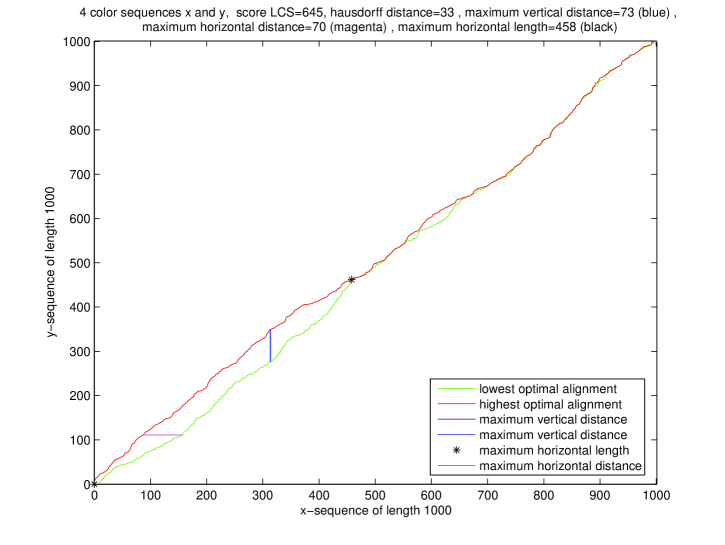
Figure 1: The extremal alignments of two independent iid four letter sequences

2.2 Related sequences

Unrelated sequences $X$ and $Y$ are independent. In our setup, the relatedness is based on the assumption that there exists a common ancestor, from which both sequences $X$ and $Y$ are obtained by independent random mutations and deletions. In the following, the common ancestor is an ${\cal A}$-valued iid process $Z_{1},Z_{2},\ldots$. A letter $Z_{i}$ has a probability to mutate according to a transition matrix that does not depend on $i$. Hence, a mutation of the letter $Z_{i}$ can be formalized as $f(Z_{i},\xi_{i})$, where $f:{\cal{A}}\times\mathbb{R}\to{\cal{A}}$ is a mapping and $\xi_{i}$ is a uniformly distributed random variable. The mapping $f_{i}(\cdot):=f(\cdot,\xi_{i})$ from ${\cal{A}}$ to ${\cal{A}}$ will be referred as the random mapping. The mutations of the letters are assumed to be independent. This means that the random variables $\xi_{1},\xi_{2},\ldots$ or the random mappings $f_{1},f_{2},\ldots$ are independent (and identically distributed). After mutations, the sequence is $f_{1}(Z_{1}),f_{2}(Z_{2}),\ldots.$ Some of its elements disappear. This is modeled via a deletion process $D^{x}_{1},D^{x}_{2},\ldots$ that is assumed to be an iid Bernoulli sequence with parameter $p$ i.e. $P(D^{x}_{i}=1)=p$. If $D^{x}_{i}=0$, then $f_{i}(Z_{i})$ is deleted. The resulting sequence, let it be $X$, is, therefore, the following: $X_{i}=f_{j}(Z_{j})$ if and only if $D^{x}_{j}=1$ and $\sum_{k=1}^{j}D^{x}_{k}=i$. Similarly, the sequence $Y$ is obtained from $Z$. For mutations, fix an iid uniformly distributed sequence $\eta_{1},\eta_{2},\ldots$ so that the mutated sequence is $h_{1}(Z_{1}),h_{2}(Z_{2}),\ldots$ with $h_{i}(\cdot):=f(\cdot,\eta_{i}).$ Note that the transition matrix corresponding to $Y$-mutations equals the one corresponding to $X$-mutations implying that the random mappings $h_{i}$ and $f_{i}$ have the same distribution. Since the mutations of $X$ and $Y$ are supposed to be independent, we assume the sequences $\xi$ and $\eta$ or the random mappings sequences $f_{1},f_{2},\ldots$ and $h_{1},h_{2},\ldots$ are independent. Note that then the pairs $(f_{1}(Z_{1}),h_{1}(Z_{1})),(f_{2}(Z_{2}),h_{2}(Z_{2})),\ldots$ are independent, but $f_{i}(Z_{i})$ and $h_{i}(Z_{i})$, in general, are not. Finally, some of the elements of $h_{1}(Z_{1}),h_{2}(Z_{2}),\ldots$ are deleted according to a deletion process $D^{y}_{1},D^{y}_{2},\ldots$ consisting of ${\it iid}$ Bernoulli random variables with the same parameter as $D^{x}$ but independent of $D^{x}.$ The remaining elements define $Y$-sequence. Note that our definition of relatedness involves the independent sequences as a special case, when the functions $f$ does not depend on $Z$.

Example: The following table illustrates the generic process of obtaining $X$ and $Y$.

$$\begin{array}[]{c|c|c|c|c|c|c|c}Z:&Z_{1}&Z_{2}&Z_{3}&Z_{4}&Z_{5}&Z_{6}&\text{common ancestor}\\ \hline\cr\\ \hline\cr f(Z):&f_{1}(Z_{1})&f_{2}(Z_{2})&f_{3}(Z_{3})&f_{4}(Z_{4})&f_{5}(Z_{5})&f_{6}(Z_{6})&\text{X mutations}\\ \hline\cr D^{x}:&0&1&1&0&0&1&\text{X deletions}\\ \hline\cr X:&&X_{1}&X_{2}&&&X_{3}&\\ \hline\cr\\ \hline\cr h(Z):&h_{1}(Z_{1})&h_{2}(Z_{2})&h_{3}(Z_{3})&h_{4}(Z_{4})&h_{5}(Z_{5})&h_{6}(Z_{6})&\text{Y mutations}\\ \hline\cr D^{y}:&1&1&1&0&1&0&\text{Y deletions}\\ \hline\cr Y:&Y_{1}&Y_{2}&Y_{3}&&Y_{4}&&\end{array}$$

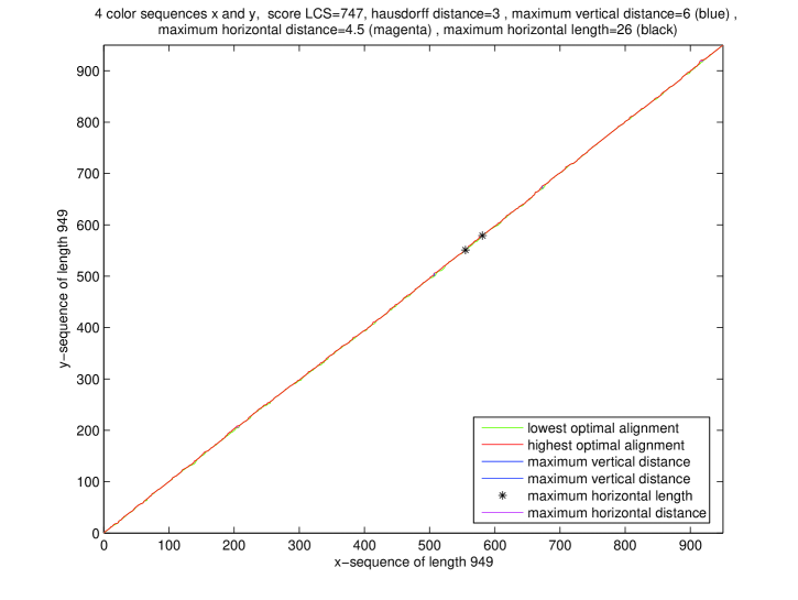
Figure 2: The extremal alignments of two related four letter sequences

In [1], the related sequences were simulated and the corresponding extremal alignments were found. Figure 2 presents a typical picture or extremal alignments of two related sequences of length 1000. Clearly the extremal alignments are close to each other; in particular the maximal vertical and horizontal distance is much smaller than these ones in Figure 1. The closeness of the extremal alignments of the related sequences follows from the main result of [1]. Before we state the result formally, some notations need to be introduced. Let $\gamma_{R}$ be the limit of (2.1), where $X$ and $Y$ are related. Typically $\gamma_{R}>\gamma$, where $\gamma$ is the limit of independent sequences with the same laws. The existence of $\gamma_{R}$ is proven in [1]. Let

$$p(a) :=P(X_{i}=a),\quad q=1-\min_{a}p(a),\quad p_{o}=P(X_{i}=Y_{i})=\sum_{a}p(a)^{2},$$

$$\bar{p} :=\max_{a\in{\cal A}}p(a),\quad\bar{q}:=1-\min_{a,b}P(X_{i}=a|Y_{i}=b),\quad\rho:={p_{0}\bar{q}\over\bar{p}q}.$$

When $X$ and $Y$ are independent, then $\bar{q}=q$. The following theorem is the main result of [1]. Below, it is stated for vertical sequence, but it also holds for horizontal distance. The condition (2.3) postulates the relatedness. It can be shown that for independent or very little related sequences (2.3) is not fulfilled. It does not mean that for independent sequences the inequality (2.4) fails, but the simulations in [1] show that this is the case. In the following theorem, $h$ stands for the binary entropy function, i.e, $h(p)=-p\log_{2}p-(1-p)\log_{2}(1-p)$.

Theorem 2.1

Let $X$ and $Y$ be related. Assume

$$\gamma_{\tt R}\log_{2}\bar{p}+(1-\gamma_{\tt R})\log_{2}(q\bar{q})+\big{(}(1-\gamma_{\tt R})\wedge\gamma_{\tt R})\log_{2}\big{(}\rho\vee 1\big{)}+2h(\gamma_{\tt R})<0.$$ (2.3)

Then there exist constants $C<\infty$ and $D<\infty$ such that for $n$ big enough,

$$P\bigl{(}V_{n}>C\ln n\bigr{)}\leq Dn^{-2},$$ (2.4)

where $V_{n}$ is the maximal vertical distance between extremal alignments.

3 The case study

Based on Theorem 2.1 as well as the simulation study, we conjecture that properties of the extremal alignments could be used as a measure of relatedness. In particular, the maximal horizontal and vertical distance between extremal alignments might me a good measure. Also, as one can see from the Figures 1 and 2 (and from other similar simulations), for independent sequences, there are relatively long intervals where the extremal alignments do not coincide. In Figure 1, the biggest such interval has length 458 (the end of that interval is marked with *). This interval is called the maximal non-uniqueness stretch, and we conjecture that this can be a good measure of homology as well. A related criterion is the number of points where the extremal alignments coincide. We call it the number of uniqueness points. Clearly in Figure 1 the number of uniqueness points is relatively small in comparison with Figure 2.

We studied four bacterial genes with comparable length (about 1500 letters). The gene is dnaA and they were taken from bacteria Pseudomonas putida F1 (Gene nr.1), Pseudomonas syringae pv. syringae B728a (Gene nr. 2), Escherichia coli E24377A (Gene nr. 3) and Erwinia carotovora subsp. atroseptica SCRI1043 (Gene nr 4). The corresponding DNA-sequences can be found in Appendix. All the genes have the same function, therefore they are presupposed similar. The results of the case study are in the following table.

Genes	1	2	3	4
Max; total	2738; 2738	1521; 1521	625; 671	529; 529
Query	100	100	71	61
E-value	0	0	2e-175	1e-146
MaxIdent	100	82	75	72
LCS	1518	1298	1081	1055
Vert+Hor=Sum	0+0=0	12+11=23	17+18=35	20+24=44
non-uniq st.	0	26	79	111
uniq points	1518	1003	604	520
Max; total	1521; 1521	2771; 2771	668; 722	538; 592
Query	100	100	70	69
E-value	0	0	0	3e-149
MaxIdent	82	100	76	73
LCS	1298	1536	1097	1071
Vert+Hor=Sum	12+11=23	0+0=0	15+13=28	14+24=38
non-uniq st.	26	0	45	80
uniq points	1003	1536	633	565
Max; total	625; 671	668; 722	2533; 2533	1323; 1323
Query	76	76	100	100
E-value	2e-175	0	0	0
MaxIdent	75	76	100	81
LCS	1081	1097	1404	1196
Vert+Hor=Sum	17+18=35	15+13=28	0+0=0	6+6=12
non-uniq st.	79	45	0	21
uniq points	604	633	1404	868
Max; total	529; 529	538; 592	1323; 1323	2522; 2522
Query	67	76	100	100
E-value	1e-146	2e-149	0	0
MaxIdent	72	73	81	100
LCS	1055	1071	1169	1398
Vert+Hor=Sum	20+24=44	14+24=38	6+6=12	0+0=0
non-uniq st.	111	80	21	0
uniq points	520	565	868	1398

In the table, every (double) cell represents several similarity criterion between two genes. In the upper part of the cell, the standard outputs of BLAST-program is represented. The entries "Max" and "Total" are the maximum and total scores, respectively; "Query" is the Query-coverage, "E-value" and "MaxIdent" are the e-value and max-ident, respectively. All parameters of BLAST were deliberately chosen default. The second half of the cell corresponds to the extremal alignments-based criterions. "LCS" stands for the length of the LCS, "Vert+Hor=Sum" is the sum of maximal vertical and horizontal distance between the extremal alignment, "non-uniq st." is the length of the longest non-uniqueness stretch and "uniq points" is the number of uniqueness points of the extremal alignments.

From the table, it is evident that Genes 1 and 2 and 3 and 4 are closely related: the maximum and total scores of BLAST between pairs (Gene 1, Gene 2) and ( Gene 3, Gene 4) are remarkably higher than the ones of any other pair of different genes. Note that this difference is also well represented by the number of uniqueness points and, remarkably well by the length of the longest non-uniqueness stretch. Also, the sums of maximum horizontal and vertical distances are in full correspondence with other criterions measuring well the degree of relatedness. Finally and, perhaps, most importantly note that all extremal alignments based criterions seem to be more sensible to the relatedness, although also the length of LCS shows the similarities rather well.

4 Appendix

Gene1: Pseudomonas putida F1

GTGTCAGTGGAACTTTGGCAGCAGTGCGTGGAGCTTCTGCGCGATGAACTGCCTGCCCAGCAATTCAACA CCTGGATCCGTCCGCTACAGGTCGAAGCCGAAGGCGACGAGTTGCGCGTCTATGCGCCTAACCGTTTCGT TCTCGATTGGGTCAATGAAAAGTACCTGGGTCGTTTGCTCGAGCTGTTGGGTGAGAACGGTAGCGGCATT GCACCAGCCCTTTCCTTATTAATAGGTAGCCGCCGCAGCTCGGCCCCAAGGGCTGCACCCAACGCGCCGG TCAGCGCTGCCGTTGCGGCTTCGCTGGCGCAGACTCAGGCGCACAAGACGGCCCCGGCAGCAGCGGTTGA ACCCGTTGCCGTGGCCGCGGCCGAGCCTGTATTGGTCGAGACGTCTTCGCGTGACAGCTTTGATGCCATG GCCGAGCCTGCTGCTGCGCCGCCCAGTGGTGGCCGGGCTGAACAGCGCACCGTGCAGGTTGAAGGTGCGC TCAAGCACACCAGTTACCTGAACCGGACCTTTACCTTTGACACCTTCGTCGAAGGTAAGTCGAACCAGCT CGCCCGCGCGGCTGCCTGGCAGGTTGCGGACAACCCTAAGCATGGCTACAACCCACTGTTCCTTTATGGC GGTGTGGGTTTGGGTAAAACCCACCTTATGCATGCTGTGGGTAACCATCTGCTGAAGAAGAATCCGAACG CCAAGGTGGTGTACCTGCATTCGGAGCGCTTCGTCGCGGACATGGTCAAAGCGTTGCAACTCAACGCCAT CAACGAATTCAAGCGCTTCTACCGCTCGGTGGACGCGTTGCTGATCGACGATATCCAGTTCTTCGCTCGC AAAGAGCGCTCGCAAGAAGAGTTTTTCCACACCTTCAACGCCTTGCTTGAGGGTGGCCAGCAGGTAATCC TTACCTCTGACCGCTATCCCAAGGAAATCGAAGGCCTGGAAGAGCGTCTGAAGTCGCGCTTTGGTTGGGG CCTGACGGTGGCTGTCGAGCCGCCAGAGCTGGAGACCCGCGTAGCGATCCTGATGAAGAAGGCCGACCAG GCCAAAGTCGAGCTCCCGCATGACGCAGCCTTTTTCATCGCTCAGCGCATCCGGTCCAACGTCCGTGAGC TGGAAGGTGCACTGAAGCGAGTTATTGCTCACTCGCACTTCATGGGGCGTGACATCACCATCGAGCTGAT TCGTGAATCGCTCAAGGATCTGTTGGCGCTGCAAGACAAACTGGTCAGTGTGGATAACATTCAGCGTACC GTCGCTGAGTACTACAAGATCAAGATCTCCGATCTGTTGTCCAAGCGTCGTTCGCGTTCTGTCGCGCGCC CGCGTCAGGTAGCCATGGCCCTGTCCAAGGAGTTGACCAACCACAGTCTGCCGGAAATCGGCGACATGTT CGGTGGTCGCGACCATACGACCGTGCTGCACGCCTGCCGCAAAATCAATGAACTGAAGGAATCCGACGCG GACATCCGCGAGGACTACAAGAACCTGCTGCGGACGCTGACGACCTGA

Gene2: Pseudomonas syringae pv. syringae B728a

GTGTCAGTGGAACTTTGGCAGCAGTGCGTGGAGCTTTTGCGCGATGAGCTGCCTGCCCAGCAATTCAACA CTTGGATCCGTCCGCTACAGGTCGAAGCCGAAGGCGACGAGTTGCGTGTGTACGCACCCAATCGTTTTGT TCTCGACTGGGTCAACGAAAAGTACCTTGGTCGTCTGCTCGAGCTTCTCGGCGAACACGGTCAAGGCATG GCCCCTGCTCTTTCCTTATTAATAGGAAGCAAGCGCAGCTCAGCACCGCGTGCTGCCCCGAATGCACCCT TGGCCGCTGCAGCCTCACAGGCGCTGTCTGCCAATTCGGTCAGCAGCGTCTCGGCCCCGGCTCCTGCCAC GGCTGCTCCAGCTGCTGCTGTAGCGACGCCTGCACCGGTTCAGAACGTTGCAACACACGACGAACCGTCG CGTGACAGCTTCGATCCGATGGCCGGAGCCAGCTCGCAACAAGCGCCCGCCCGCGCTGAACAACGTACCG TCCAGGTAGAAGGTGCGCTCAAGCACACCAGTTACCTGAACCGTACGTTCACGTTCGAAAATTTCGTCGA GGGTAAGTCCAACCAGCTGGCACGCGCTGCGGCCTGGCAGGTTGCCGACAACCCCAAGCATGGCTACAAC CCGCTGTTCCTTTATGGCGGCGTGGGTCTTGGTAAAACTCACTTGATGCATGCGGTGGGTAACCACCTGC TGAAGAAGAACCCGAACGCCAAGGTCGTGTACCTGCATTCGGAGCGCTTCGTTGCAGACATGGTCAAGGC CTTGCAGCTCAATGCAATCAACGAGTTCAAGCGCTTCTACCGTTCAGTCGATGCGCTGCTGATCGACGAC ATCCAGTTTTTTGCCCGCAAGGAACGTTCGCAGGAAGAGTTTTTCCACACGTTCAACGCGCTGCTGGAAG GCGGACAGCAGGTCATTCTGACCAGCGACCGCTATCCCAAGGAAATCGAAGGCCTTGAAGAGCGACTCAA ATCGCGTTTTGGCTGGGGCCTGACGGTTGCCGTCGAGCCTCCGGAGCTGGAAACCCGCGTGGCGATCCTC ATGAAAAAAGCAGATCAGGCCAAGGTCGATCTGCCCCATGACGCAGCGTTCTTCATCGCCCAGCGAATTC GCTCCAACGTCCGTGAGCTGGAAGGTGCGCTCAAGCGCGTCATCGCTCACTCGCACTTCATGGGCCGCGA CATCACCATCGAGCTGATTCGCGAGTCGCTGAAGGACTTGCTGGCGTTGCAGGACAAGCTGGTCAGTGTG GATAACATTCAGCGCACTGTCGCCGAGTACTACAAGATCAAGATTTCCGATCTGCTGTCCAAGCGTCGTT CCCGCTCTGTCGCCCGGCCTCGTCAGGTCGCGATGGCGCTCTCCAAGGAACTCACCAACCACAGTCTTCC GGAAATCGGTGACGTGTTTGGTGGCCGTGACCACACGACTGTCTTGCACGCATGCCGAAAGATCAACGAG CTCAAGGAATCCGATGCGGATATCCGCGAGGACTACAAGAACCTGCTGCGCACTCTGACTACGTGA

Gene3: Escherichia coli E24377A

GTGTCACTTTCGCTTTGGCAGCAGTGTCTTGCCCGATTGCAGGATGAGTTACCAGCCACAGAATTCAGTA TGTGGATACGCCCATTGCAGGCGGAACTGAGCGATAACACGCTGGCCCTGTACGCGCCAAACCGTTTTGT CCTCGATTGGGTACGGGACAAGTACCTTAATAATATCAATGGACTGCTAACCAGTTTCTGCGGAGCGGAT GCCCCACAGCTGCGTTTTGAAGTCGGCACCAAACCGGTGACGCAAACGCCACAAGCGGCAGTGACGAGCA ACGTCGCGGCCCCTGCACAGGTGGCGCAAACGCAGCCGCAACGTGCTGCGCCTTCTACGCGCTCAGGTTG GGATAACGTCCCGGCCCCGGCAGAACCGACCTATCGTTCTAACGTAAACGTCAAACACACGTTTGATAAC TTCGTTGAAGGTAAATCTAACCAACTGGCGCGCGCGGCGGCTCGCCAGGTGGCGGATAACCCTGGCGGTG CCTATAACCCGTTGTTCCTTTATGGCGGCACGGGTCTGGGTAAAACTCACCTGCTGCATGCGGTGGGTAA CGGCATTATGGCGCGCAAGCCGAATGCCAAAGTGGTTTATATGCACTCCGAGCGCTTTGTTCAGGACATG GTTAAAGCCCTGCAAAACAACGCGATCGAAGAGTTTAAACGCTACTACCGTTCCGTAGATGCACTGCTGA TCGACGATATTCAGTTTTTTGCTAATAAAGAACGATCTCAGGAAGAGTTTTTCCACACCTTCAACGCCCT GCTGGAAGGTAATCAACAGATCATTCTCACCTCGGATCGCTATCCGAAAGAGATCAACGGCGTTGAGGAT CGTTTGAAATCCCGCTTCGGTTGGGGACTGACTGTGGCGATCGAACCGCCAGAGCTGGAAACCCGTGTGG CGATCCTGATGAAAAAGGCCGACGAAAACGACATTCGTTTGCCGGGTGAAGTGGCGTTCTTTATCGCCAA GCGTCTACGATCTAACGTACGTGAGCTGGAAGGGGCGCTGAACCGCGTCATTGCCAACGCCAACTTTACC GGAAGGGCGATCACCATCGACTTCGTGCGTGAGGCGCTGCGCGACTTGCTGGCATTGCAGGAAAAACTGG TCACCATCGACAATATTCAGAAGACGGTGGCGGAGTACTACAAGATCAAAGTTGCGGATCTCCTTTCCAA GCGTCGATCCCGCTCGGTGGCGCGTCCGCGCCAGATGGCGATGGCGCTGGCGAAAGAGCTGACTAACCAC AGTCTGCCGGAGATTGGCGATGCGTTTGGTGGTCGTGACCACACGACGGTGCTTCATGCCTGCCGTAAGA TCGAGCAGTTGCGTGAAGAGAGCCACGATATCAAAGAAGATTTTTCAAATTTAATCAGAACATTGTCATC GTAA

Gene4: Erwinia carotovora subsp. atroseptica SCRI1043

GTGTCACTTTCGCTTTGGCAGCAGTGTCTTGCCCGTTTGCAGGATGAGTTACCTGCCACAGAATTCAGTA TGTGGATACGCCCGTTGCAGGCGGAACTGAGTGATAACACTCTGGCGCTCTACGCCCCCAATCGCTTTGT GCTGGATTGGGTTCGTGATAAATACTTAAATAATATCAATGTCCTGCTGAATGATTTTTGCGGGATGGAT GCCCCCTTACTGCGTTTTGAAGTGGGGAGTAAACCGCTGGTTCAAACCATAAGCCAGCCAGCGCAGTCGC ACCACAACCCTGTCAGCGTTGCACGGCAACAGCCAGTACGCATGGCACCGGTACGCCCAAGCTGGGATAA CTCGCCTGTACAGGCAGAGCATACCTACCGTTCCAATGTGAACCCGAAACATACGTTTGATAACTTCGTT GAGGGTAAATCGAACCAGTTAGCACGGGCAGCGGCACGTCAGGTGGCTGACAACCCAGGCGGCGCGTATA ACCCGCTGTTTCTCTATGGCGGCACTGGCTTGGGTAAAACGCACCTGTTGCATGCAGTGGGGAATGGTAT TATCGCCCGTAAACCCAACGCGAAGGTGGTCTACATGCACTCCGAGCGTTTCGTGCAGGATATGGTGAAG GCGTTGCAGAACAATGCGATTGAAGAGTTCAAACGCTACTACCGTTCTGTTGACGCACTGCTGATCGATG ATATTCAATTCTTCGCTAATAAAGAGCGTTCGCAGGAAGAGTTCTTTCATACCTTTAATGCACTGCTGGA AGGCAACCAGCAAATCATTCTGACTTCTGACCGCTACCCGAAAGAGATCAATGGTGTGGAAGATCGTCTA AAATCCCGCTTTGGTTGGGGGTTAACGGTCGCGATTGAACCGCCTGAGCTGGAAACCCGCGTGGCGATTC TGATGAAAAAGGCAGATGAAAATGACATTCGCTTGCCTGGTGAAGTCGCATTCTTTATTGCTAAACGCCT GCGTTCTAACGTGCGTGAGTTGGAAGGTGCATTGAACCGCGTTATTGCTAACGCCAATTTTACCGGCCGT TCGATCACCATTGATTTTGTGCGTGAGGCGCTGCGCGATCTGCTGGCGTTGCAGGAAAAGCTGGTTACTA TCGACAATATTCAAAAGACCGTGGCGGAATACTATAAAATCAAGATAGCCGACCTGCTGTCTAAACGACG TTCCCGCTCGGTGGCGCGTCCGCGCCAGATGGCGATGGCGTTGGCGAAAGAACTGACGAATCACAGCCTG CCGGAAATTGGCGATGCCTTTGGCGGGCGTGATCATACGACGGTGTTGCATGCCTGCCGCAAGATTGAGC AGTTGCGTGAAGAAAGCCACGACATCAAAGAAGATTTTTCCAATTTAATCAGAACACTATCGTCATAA

References

- [1] Lember, Jüri, Matzinger, Heinrich and Vollmer, Anna-Lisa . Optimal alignments of longest common subsequence and their path properties. (2012), submitted.
- [2] Kun-Mao Chao, Louxin Zhang. Sequence Comparison: Theory and Methods. Springer, (2009).
- [3] Durbin, R. and Eddy, S. and Krogh A. and Mitchison, G.. Biological Sequence Analysis: Probabilistic Models of Proteins and Nucleic Acids, Cambridge University Press, (1998).
- [4] Waterman, Michael S. and Vingron, M. Sequence Comparison Significance and Poisson Approximation. Statistical Science, 9 (1994), 367–381.
- [5] Arratia, Richard and Waterman, Michael S.. A phase transition for the score in matching random sequences allowing deletions. Ann. Appl. Probab. 4 (1994), 200–225.
- [6] Waterman, Michael S. Introduction to Computational Biology, Chapman & Hall, (1995).
- [7] http://blast.ncbi.nlm.nih.gov/Blast.cgi