Quasinormal frequencies using the hidden conformal symmetry of the Schwarzschild black hole

Yong-Wan Kim ^1,a, Yun Soo Myung^2,b, and Young-Jai Park^1,3,c

¹ Center for Quantum Spacetime, Sogang University, Seoul 121-742, Korea

²Institute of Basic Science and School of Computer Aided Science,

Inje University, Gimhae 621-749, Korea

³Department of Physics and Department of Global Service Management,

Sogang University, Seoul 121-742, Korea

Abstract

We show that the hidden conformal symmetry of the Schwarzschild black hole is realized from the AdS₂ sector of the AdS${}_{2}\times S^{2}$, but not from the Rindler spacetime which is the genuine near-horizon geometry of the Schwarzschild black hole. This implies that purely imaginary quasinormal frequencies obtained using the hidden conformal symmetry is not suitable for describing the largely damped modes around the Schwarzschild black hole.

PACS numbers: 04.70.Dy, 04.70.Bw, 04.30.Nk, 04.70.-s
Keywords: Hidden conformal symmetry, Quasinormal modes, Black Holes

^aywkim65@gmail.com
^bysmyung@inje.ac.kr
^cyjpark@sogang.ac.kr

1 Introduction

Recently, it was shown that an SL(2,R) hidden conformal symmetry [1] could be realized in a scalar wave equation around the Schwarzschild black hole when taking the near-region and low-energy limits [2]. We refer to the geometry modified in this way as the subtracted geometry which shows that it has the same near-horizon properties as the original Schwarzschild black hole, but different asymptotes at infinity [3]. Actually, it does not have an asymptotically flat spacetime implied by the Schwarzschild black hole but it has an asymptotically anti-de Sitter (AdS) spacetime.

Importantly, it was claimed that a hidden conformal symmetry has been used to derive purely imaginary quasinormal frequencies (QNFs) by using the operator method. However, we wish to clarify that the Rindler space is the truly near-horizon geometry of the Schwarzschild black hole, while the near-region and low-energy limits of the wave equation around the Schwarzschild spacetime corresponds to the wave equation around the AdS segment of the AdS${}_{2}\times S^{2}$, which is inspired by the near-extremal Reissner-Nordström (RN) black hole [4]. Here the near-horizon geometry (region) means $r\approx r_{+}$, while both the near-region ($\omega r\ll 1$) and the low-energy limit ($\omega r_{+}\ll 1$) [5] are necessary to develop a hidden conformal symmetry in a scalar wave equation. The AdS segment shrinks to the Rindler space for the non-extremal Schwarzschild black hole, whereas it grows to the AdS space for the near-extremal RN black hole.

On the other hand, it seems difficult to derive QNFs of a scalar propagating on the Schwarzschild black hole by using a hidden conformal symmetry solely. As is well known, quasinormal modes will be determined by solving a scalar wave equation around the Schwarzschild black hole as well as imposing the boundary conditions: ingoing waves at the horizon and outgoing waves at infinity. We stress that any restriction on the frequency $\omega$ is not allowed for deriving quasinormal modes. Purely imaginary QNFs were found by employing the operator method developed in the subtracted geometry [3]. In this case, the ingoing waves at the horizon were guaranteed, but quasinormal modes do not satisfy the outgoing wave-boundary condition because these modes were developed using the near-region and low-energy limits [2] where the frequency $\omega$ should satisfy inequalities of $\omega\ll 1/r$ and $\omega\ll 1/r_{+}$. Furthermore, it was suggested that purely imaginary QNFs ($\omega_{n}$) in Eq. (37) yield the correct leading behavior of $\omega$ in Eq. (38) for large damping with large overtone number $n$. However, we observe from Eq. (37) that the important differences are the absence of real part, the non-large overtone number $n$, and the appearance of angular momentum number $l$ in the imaginary part. In view of these, purely imaginary QNFs may not be acceptable as QNFs describing a scalar perturbation around the Schwarzschild black hole because the outgoing boundary condition is not imposed at infinity.

A promising case was found in the RN black hole. We have derived the purely imaginary QNFs of the RN black hole by making use of a hidden conformal symmetry developed in the near-region and low-energy limits of the scalar equation [6]. We are aware that the operator approach has a limitation because the $\omega$-dependent potential is approximated by a single term of a hidden conformal symmetry potential. This means that developing a hidden conformal symmetry in the near-horizon region means neglecting the large $r>r_{+}$ behavior of the potential in the whole RN black hole spacetime and thus, leading to the subtracted geometry. Fortunately, it was known that purely imaginary QNFs could be also obtained from a scalar perturbation around the near-extremal RN black hole without any modifications [7]. This implies that the subtracted geometry [=near-extremal RN black hole] is the solution to the original Einstein-Maxwell theory which provides the RN black hole.

It is worth noting that both the near-horizon and asymptotic geometries (whole information) are necessary to derive QNFs, even though the entropy counting for a black hole may require the near-horizon geometry only [3, 8]. In fact, it shows different utilities of the hidden conformal symmetry in deriving between QNFs and entropy. Hence we propose that if one obtains QNFs (purely imaginary QNFs) using the hidden conformal symmetry based on the subtracted geometry, one has to find the corresponding black hole (near-extremal RN black hole) where the same QNFs will be found by solving the scalar equation as well as imposing two boundary conditions without taking any limits.

One counter example is the Schwarzschild black hole. In this case, the subtracted geometry [=near-extremal RN black hole] is not the solution to the original Einstein theory which provides the Schwarzschild black hole. We would like to stress that the Rindler spacetime is the near-horizon solution to the Einstein theory which gives us the Schwarzschild black hole.

In this work, we will show that purely imaginary QNFs obtained using a hidden conformal symmetry are not suitable for describing largely damped modes around the Schwarzschild black hole.

2 Hidden conformal symmetry in the subtracted geometry

Let us begin with the Schwarzschild metric given by

$$ds^{2}_{\rm Sch}=-f(r)dt^{2}+\frac{dr^{2}}{f(r)}+r^{2}d\Omega^{2}_{2},$$ (1)

where $f(r)=1-r_{+}/r$ with $r_{+}=2M$. Here, $M$ is the ADM mass and the surface gravity is

$$\kappa=\frac{1}{4M}=2\pi T_{H}$$ (2)

with the Hawking temperature $T_{H}$.

The Klein-Gordon equation for a massless scalar is given by

$$\bar{\square}_{\rm Sch}\Phi=0.$$ (3)

Expanding in eigenmodes of

$$\Phi(t,r,\theta,\phi)=e^{-i\omega t}\frac{R(r)}{r}Y^{l}_{m}(\theta,\phi)\ ,$$ (4)

and using the tortoise coordinate defined by

$$r_{*}=\int\frac{dr}{f(r)}=r+r_{+}\ln\left(\frac{r}{r_{+}}-1\right),$$ (5)

the radial part of Eq. (3) becomes the Schrödinger-type equation

$$\frac{d^{2}}{dr_{*}^{2}}R(r)+\Big{[}\omega^{2}-V_{\rm Sch}(r)\Big{]}R(r)=0,$$ (6)

where the potential is given by

$$V_{\rm Sch}(r)=f(r)\Big{[}\frac{l(l+1)}{r^{2}}+\frac{2M}{r^{3}}\Big{]}.$$ (7)

On the other hand, the approximated Klein-Gordon equation could be expressed in terms of the eigenvalue equation [2]

$${\cal H}^{2}\Phi = \left(r^{2}f(r)\partial^{2}_{r}+2(r-M)\partial_{r}-\frac{16M^{4}}{r^{2}f(r)}\partial^{2}_{t}\right)\Phi$$ (8)

$$= l(l+1)\Phi$$

which is designed for describing a scalar propagating on the Schwarzschild spacetime in the near-region and low-energy limits. Note that the SL(2,R) Casimir operator ${\cal H}^{2}$ is given by

$${\cal H}^{2}=-H^{2}_{0}+\frac{1}{2}\Big{(}H_{1}H_{-1}+H_{-1}H_{1}\Big{)},$$ (9)

where three operators

$$H_{\pm 1} = \pm ie^{\pm t/4M}\Big{(}\Delta^{1/2}\partial_{r}\mp 4M(r-M)\Delta^{-1/2}\partial_{t}\Big{)},$$

$$H_{0} = -4iM\partial_{t}\leavevmode\nobreak\ \leavevmode\nobreak\ \leavevmode\nobreak\ {\rm with}\leavevmode\nobreak\ \Delta=r^{2}f(r)$$ (10)

obey the SL(2,R) commutation relations:

$$\Big{[}H_{0},H_{\pm 1}\Big{]}=\mp iH_{\pm 1},\leavevmode\nobreak\ \leavevmode\nobreak\ \Big{[}H_{1},H_{-1}\Big{]}=2iH_{0}.$$ (11)

In order to investigate what happens when the near-region and low-energy limits are taken into account, we rewrite the approximated Klein-Gordon equation (8) by using the tortoise coordinate $r_{*}$ as

$$\frac{d^{2}}{dr_{*}^{2}}R(r)+\Big{[}\omega^{2}-V_{\omega}(r)\Big{]}R(r)=0,$$ (12)

where the $\omega$-dependent potential

$$V_{\omega}(r)=\omega^{2}\left(1-\frac{r^{4}_{+}}{r^{4}}\right)+V_{\rm Sch}(r)$$ (13)

has an additional term to the original potential $V_{\rm Sch}(r)$. Since the potential $V_{\rm Sch}(r)$ contains all information for the Schwarzschild black hole spacetime where a scalar propagates on, the appearance of $\omega^{2}$-dependent term is unusual and thus, it reflects the near-region and low-energy limits. We observe that the $\omega^{2}$-dependent term arises from when replacing five terms in $\omega^{2}r^{4}/\Delta$ with a single term $\omega^{2}r^{4}_{+}/\Delta$ [2], which is regarded as a key step to develop the hidden conformal symmetry in the Schwarzschild spacetime. This replacement is done when taking the near-region limit ($\omega r\ll 1$) and low-energy limit ($\omega r_{+}\ll 1$). If one does not take these limits, the $r_{+}$ in the $\omega^{2}$-dependent term goes back to $r$ and thus, the $\omega^{2}$-dependent term disappears. This implies that $V_{\omega}(r)$ leads to $V_{\rm Sch}(r)$ for $r\to r_{+}$. In Fig. 1, we depict the four potentials which consist of $V_{\rm Sch}(r)$ and three $V_{\omega}(r)$ for $\omega=0.1,\leavevmode\nobreak\ 0.2,\leavevmode\nobreak\ 0.3$. The figure shows that in the near-horizon limit ($r\to r_{+}=2$), all the potentials have the nearly same form, irrespective of $\omega^{2}$ but for $r>r_{+}$, they have different forms depending on $\omega^{2}$. Hence, we observe that for $r\approx r_{+}$, $V_{\omega}(r)\approx V_{\rm Sch}(r)$ for any $\omega$. When $\omega$ approaches zero, $V_{\omega}(r)$ recovers the original potential $V_{\rm Sch}(r)$. However, it is worth noting that the near-horizon region of $r\approx r_{+}$ is not enough to derive the quasinormal modes because two boundary conditions are required. Definitely, one observes a difference between $V_{\rm Sch}(r)\sim 0$ and $V_{\omega}(r)\sim\omega^{2}$ for large $r$.

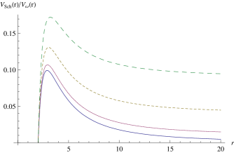
Figure 1: Different potentials for $M=l=1$ in the Schwarzschild coordinate $r$. The bottom curve depicts the Schwarzschild potential $V_{\rm Sch}(r)$, while three others are the $\omega$-dependent potential $V_{\omega}(r)$ for $\omega$=0.3, 0.2, and 0.1 from top to bottom. For large $r$, one observes that $V_{\rm Sch}(r)\sim 0$, while $V_{\omega}(r)\sim\omega^{2}$.

In order to describe the near-horizon region well, it is convenient to introduce a new coordinate defined by

$$\rho\equiv-\frac{1}{2\kappa}\ln\Big{[}1-\frac{r_{+}}{r}\Big{]}.$$ (14)

In terms of $\rho$, the event horizon $r_{+}$ is mapped into $\rho\rightarrow\infty$, while the spatial infinity $r\rightarrow\infty$ into $\rho\rightarrow 0$: $r\in[r_{+},\infty]$ is inversely mapped into $\rho\in[\infty,0]$. Using the coordinate (14), the Schwarzschild metric becomes

$$ds^{2}_{\rm\rho}=-\tilde{f}(\rho)dt^{2}+\tilde{f}^{-1}(\rho)\left(\frac{r_{+}}{2\sinh(\kappa\rho)}\right)^{2}\left[\left(\frac{\kappa}{\sinh(\kappa\rho)}\right)^{2}d\rho^{2}+d\Omega^{2}\right]$$ (15)

with

$$\tilde{f}(\rho)=e^{-2\kappa\rho}.$$ (16)

Then, making use of the ansatz

$$\Phi(t,\rho,\theta,\phi)=e^{-i\omega t}R(\rho)Y^{l}_{m}(\theta,\phi)\ ,$$ (17)

the massless scalar propagating in the spacetime (15) satisfies

$$\Big{(}\frac{\sinh(\kappa\rho)}{\kappa}\Big{)}^{2}\frac{d^{2}}{d\rho^{2}}R(\rho)+\left[\frac{\omega^{2}}{\tilde{f}^{2}(\rho)}\Big{(}\frac{r_{+}}{2\sinh(\kappa\rho)}\Big{)}^{2}-l(l+1)\right]R(\rho)=0.$$ (18)

This can be rewritten as the Schrödinger-type equation

$$\frac{d^{2}}{d\rho^{2}}R(\rho)+\Big{[}\omega^{2}-\tilde{V}_{\rm\omega}(\rho)\Big{]}R(\rho)=0.$$ (19)

Here the $\omega$-dependent potential is given by

$$\tilde{V}_{\rm\omega}(\rho)=\omega^{2}\Big{[}1-\frac{1}{16\tilde{f}^{2}(\rho)\sinh^{4}(\kappa\rho)}\Big{]}+\frac{l(l+1)\kappa^{2}}{\sinh^{2}(\kappa\rho)}.$$ (20)

We note a useful relation between $r$ and $\rho$

$$\left(\frac{r_{+}}{r}\right)^{4}=16\tilde{f}^{2}(\rho)\sinh^{4}(\kappa\rho).$$ (21)

In the limits of the near-region ($\rho\rightarrow\infty$) and low-energy ($\omega\to 0$), the square bracket in (20) is approximated to be zero as

$$\omega^{2}\Big{[}1-\frac{1}{16\tilde{f}^{2}(\rho)\sinh^{4}(\kappa\rho)}\Big{]}\sim\frac{\omega^{2}}{\sinh^{2}(\kappa\rho)}\sim 0.$$ (22)

Thus, in these limits, the $\omega$-dependent potential $\tilde{V}_{\omega}$ (20) reduces to a single term

$$V_{\rm HCS}(\rho)=\frac{l(l+1)\kappa^{2}}{\sinh^{2}(\kappa\rho)}.$$ (23)

We note that this potential is not the original potential $\tilde{V}_{\omega}$. This is just an approximated potential to explore the hidden conformal symmetry in the near-horizon region of the Schwarzschild spacetime. Hence, we have the subtracted geometry when using $V_{\rm HCS}$ instead of $\tilde{V}_{\omega}$. Its near-horizon and asymptotic forms take $V_{\rm HCS}(\rho\to\infty)\sim e^{-2\kappa\rho}$ and $V_{\rm HCS}(\rho\to 0)\sim\frac{1}{\rho^{2}}$, which show that $V_{\rm HCS}(\rho)$ is similar to the potential of a scalar field around the AdS-black hole. This suggests that its asymptote is changed from a flat spacetime implied by the Schwarzschild black hole to an AdS spacetime.

In order to exhibit the hidden conformal structure, we construct three vectors defined as

$$H_{1/-1} = \frac{i}{\kappa}e^{\pm\kappa t}\Big{[}\cosh(\kappa\rho)\partial_{t}\pm\sinh(\kappa\rho)\partial_{\rho}\Big{]},$$

$$H_{0} = -\frac{i}{\kappa}\partial_{t},$$ (24)

which satisfy the SL(2,R) algebra (11). Then, the SL(2,R) Casimir operator is given by

$${\cal H}^{2}=-\Big{[}\frac{\sinh(\kappa\rho)}{\kappa}\Big{]}^{2}\partial^{2}_{t}+\Big{[}\frac{\sinh(\kappa\rho)}{\kappa}\Big{]}^{2}\partial^{2}_{\rho}.$$ (25)

As a result, the Schrödinger equation (19) with $V_{\rm HCS}(\rho)$ in Eq. (23) instead of $\tilde{V}_{\omega}(\rho)$ is equivalent to the eigenvalue equation

$${\cal H}^{2}\Phi=l(l+1)\Phi.$$ (26)

Now, one may use the hidden conformal symmetry to derive QNFs of the Schwarzschild black hole represented by the subtracted geometry. We start with the primary state given by

$$H_{0}\Phi^{(0)}=ih\Phi^{(0)}$$ (27)

which satisfies the highest weight condition

$$H_{1}\Phi^{(0)}=0.$$ (28)

Then, using the ansatz

$$\Phi^{(0)}=e^{-i\omega_{0}t}R^{(0)}(\rho)Y^{l}_{m}(\theta,\phi),$$ (29)

one has a conformal weight

$$h=i\frac{\omega_{0}}{\kappa}=i\frac{\omega_{0}}{2\pi T_{H}}.$$ (30)

On the other hand, the SL(2,R) Casimir operator satisfies

$${\cal H}^{2}\Phi^{(0)}=h(h+1)\Phi^{(0)}.$$ (31)

Comparing Eq. (31) with Eq. (26), one has

$$h=\frac{1}{2}[1\pm(2l+1)],$$ (32)

and thus, one finds

$$\omega_{0}=-i\frac{\kappa}{2}[1\pm(2l+1)].$$ (33)

Since the QNFs are purely imaginary $\omega_{I}>0\leavevmode\nobreak\ (\omega=\omega_{R}-i\omega_{I})$ with $\omega_{R}=0$, we choose the upper sign as

$$\omega_{0}=-i\kappa(l+1).$$ (34)

All the descendants can be constructed by acting the operator $H_{-1}$ on $\Phi^{(0)}$

$$\Phi^{(n)}=(-iH_{-1})^{n}\Phi^{(0)}$$ (35)

so that we have

$$\Phi^{(n)}=e^{-i\omega_{n}t}R^{(n)}(\rho)Y^{l}_{m}(\theta,\phi).$$ (36)

Here the QNFs could be read off as

$$\omega_{n}=\omega_{0}-i\kappa n=-i\kappa\Big{[}n+l+1\Big{]},\leavevmode\nobreak\ \leavevmode\nobreak\ \leavevmode\nobreak\ n\in Z^{+}$$ (37)

which are purely imaginary.

On the other hand, numerical computations of the QNFs for the Schwarzschild black hole in the limit of large damping is given by [9, 10]

$$\omega=(1.098612\cdots)T_{H}-i2\pi T_{H}\Big{(}n+\frac{1}{2}\Big{)},$$ (38)

where the real part approaches a constant of $\ln(3)$ [11], while the imaginary part becomes equally spaced with large $n$ ($\omega_{I}\gg 1$). Comparing (37) with the highly damped frequencies (38), one may see apparently that the leading behavior of $i2\pi T_{H}n$ for large damping comes out correctly. However, we observed from (38) that the important differences are the absence of real part, the non-large $n$, and the appearance of $l$ in the imaginary part. These show that the QNFs $\omega_{n}$ are not suitable for describing the scalar perturbation absorbing into the black hole.

Moreover, the $n$-th radial eigenfunction $R^{(n)}(\rho)$ is constructed as

$$R^{(n)}(\rho) = \left(\kappa\right)^{-n}\left(-i\omega_{n-1}\cosh\left(\kappa\rho\right)-\sinh\left(\kappa\rho\right)\frac{d}{d\rho}\right)$$ (39)

$$\leavevmode\nobreak\ \times\left(-i\omega_{n-2}\cosh\left(\kappa\rho\right)-\sinh\left(\kappa\rho\right)\frac{d}{d\rho}\right)$$

$$\leavevmode\nobreak\ \cdot\cdot\cdot\times\left(-i\omega_{0}\cosh\left(\kappa\rho\right)-\sinh\left(\kappa\rho\right)\frac{d}{d\rho}\right)R^{(0)}(\rho),$$

which may be regarded as the $n$-th radial quasinormal modes. We note that $\Phi^{(n)}$ forms a principally discrete highest weight representation of the SL(2,R)

$$H_{0}\Phi^{(n)}=i(h+n)\Phi^{(n)}.$$ (40)

On the other hand, the highest weight condition (28) provides the radial solution

$$R^{(0)}(\rho)=C\Big{[}\sinh\left(\kappa\rho\right)\Big{]}^{i\frac{\omega_{0}}{\kappa}}.$$ (41)

Near the horizon of $\rho\to\infty\leavevmode\nobreak\ (r_{*}\to-\infty)$, the solution (41) behaves as

$$R^{(0)}(\rho)\sim e^{i\omega_{0}\rho},$$ (42)

showing that this is the outgoing mode ($\rightarrow$) into the horizon which is equivalent to the ingoing mode ($\leftarrow$) at the horizon when using the tortoise coordinate $r_{*}$ in Eq. (5). We observe that $R^{(0)}(0)\sim 0$, which may show that it is not the outgoing wave at infinity but it satisfies the Dirichlet boundary condition at the infinity of AdS spacetime.

Furthermore, the first radial eigenfunction $R^{(1)}(\rho)$ can be explicitly constructed as

$$R^{(1)}(\rho)=\begin{cases}-2iC\omega_{0}\cosh(\kappa\rho)\Big{[}\sinh\left(\kappa\rho\right)\Big{]}^{i\frac{\omega_{0}}{\kappa}}&\sim\leavevmode\nobreak\ \leavevmode\nobreak\ 0\leavevmode\nobreak\ \leavevmode\nobreak\ \,{\rm as\leavevmode\nobreak\ }\rho\rightarrow 0,\\ -2iC\omega_{0}\coth(\kappa\rho)\Big{[}\sinh\left(\kappa\rho\right)\Big{]}^{i\frac{\omega_{1}}{\kappa}}&\sim\leavevmode\nobreak\ \leavevmode\nobreak\ e^{i\omega_{1}\rho}\leavevmode\nobreak\ \leavevmode\nobreak\ {\rm as\leavevmode\nobreak\ }\rho\rightarrow\infty,\end{cases}$$ (43)

which show that at infinity $R^{(1)}(\rho)$ satisfies the Dirichlet boundary condition, while near the horizon $R^{(1)}(\rho)$ remains to be the outgoing mode. One can easily show that the $n$-th radial eigenfunction $R^{(n)}(\rho)$ behaves as the same way as $R^{(1)}(\rho)$ by induction.

In order to obtain the truly QNFs, we have to impose the two boundary conditions: outgoing mode near the horizon ($\rho\to\infty$) and ingoing mode at infinity ($\rho\to 0$). However, we point out that $R^{(n)}(\rho)$ do not satisfy the ingoing boundary condition at infinity because they are the solutions which were obtained by considering the subtracted geometry. Curiously, we observe that $R^{(n)}(\rho)\sim 0$ as $\rho\rightarrow 0$, which implies that in this framework, one could not impose the ingoing boundary condition at infinity. In this sense, we could not regard (37) as the truly QNFs which describe the largely damped modes around the Schwarzschild black hole because we have considered the subtracted geometry.

3 QNFs of scalar around AdS-segment

In this section, we show explicitly that the approximated potential (23) comes from the AdS₂-segment inspired by the fact that AdS${}_{2}\times S^{2}$ is the near-extremal RN black hole, but not from the Rindler space which is the genuine near-horizon geometry of the Schwarzschild spacetime. This implies that we will no longer use the subtracted geometry to derive the QNFs of scalar around the Schwarzschild black hole.

First of all, we mention that the near-horizon geometry of the Schwarzschild spacetime is a product of the Rindler space and a two sphere $S^{2}$. This can be easily realized when using the coordinate transformations

$$\hat{t}=\frac{t}{2r_{+}},\leavevmode\nobreak\ \leavevmode\nobreak\ \leavevmode\nobreak\ r=r_{+}\left(1+\frac{\eta^{2}}{4}\right).$$ (44)

The Schwarzschild spacetime (1) is turned out to be the Rindler spacetime

$$ds^{2}_{\rm RS}=r^{2}_{+}\Big{(}-\eta^{2}d\hat{t}^{2}+d\eta^{2}+d\Omega^{2}_{2}\Big{)}$$ (45)

in the near-horizon region. Note that it is impossible to develop a hidden conformal symmetry in the Rindler spacetime as will be shown in the next section.

For reference, we introduce the RN spacetime described by

$$ds^{2}_{\rm RN}=-f(r)dt^{2}+f^{-1}(r)dr^{2}+r^{2}d\theta^{2}+r^{2}d\Omega^{2}_{2},$$ (46)

where the metric function with mass $M$ and charge $Q$ is given by

$$f(r)=1-\frac{2M}{r}+\frac{Q^{2}}{r^{2}}.$$ (47)

The inner ($r_{-}$) and the outer ($r_{+}$) horizons are obtained as

$$r_{\pm}=M\pm\sqrt{M^{2}-Q^{2}}\equiv M\pm r_{0},$$ (48)

which satisfy $f(r_{\pm})=0$. We note that $r_{0}$ is a non-extremal parameter, but a very small $r_{0}\ll M(\sim Q)$ corresponds to the near-extremal RN black hole. Also, we have an extremal RN black hole for $r_{0}=0$.

On the other hand, the AdS₂-segment [4, 12] is introduced to be

$$ds^{2}_{\rm AdS}=Q^{2}\Big{(}-\sinh^{2}\!\!\eta\,d\hat{t}^{2}+\frac{\cosh^{2}\!\!\eta}{\sinh^{2}\!\!\eta+r^{2}_{0}}d\eta^{2}+d\Omega^{2}_{2}\Big{)},$$ (49)

which describes the near-extremal RN black hole. We note here that for $r_{0}=1$ [4], (49) reduces to the near-horizon geometry (AdS${}_{2}\times S^{2}$, Bertotti-Robinson spacetime) of the extremal RN black hole [13, 14]

$$ds^{2}_{\rm ERN}=Q^{2}\Big{(}-\sinh^{2}\!\!\eta\,d\hat{t}^{2}+d\eta^{2}+d\Omega^{2}_{2}\Big{)},$$ (50)

which is a solution to the Einstein-Maxwell theory. In this extremal case, its Hawking temperature is zero and its QNFs are not defined properly [7]. The spacetime is described by Ricci scalars

$$R_{AdS_{2}}=-\frac{2}{Q^{2}},\leavevmode\nobreak\ \leavevmode\nobreak\ R_{S^{2}}=\frac{2}{Q^{2}},\leavevmode\nobreak\ \leavevmode\nobreak\ R=R_{AdS_{2}}+R_{S^{2}}=0.$$ (51)

It is clear that (50) could not describe the near-extremal RN black hole because it contains only $Q$ when comparing to (49) with two parameters $Q$ and $r_{0}$.

We are interested in obtaining QNFs of scalar around the black hole with non-zero Hawking temperature. Hence, we require $r_{0}\not=1$. In fact, in the limit of $\eta\rightarrow 0$ together with $r_{0}=1$ and $Q=r_{+}$, (49) reduces to the Rindler metric (45). In order to make a further connection to the near-extremal RN black hole, we introduce the coordinate transformations

$$\sinh^{2}\!\!\eta=\tilde{\rho}^{2}-r^{2}_{0},\leavevmode\nobreak\ \leavevmode\nobreak\ \leavevmode\nobreak\ \hat{t}=\frac{t}{Q^{2}}.$$ (52)

Then, one can obtain the near-extremal RN black hole with $r_{0}=(r_{+}-r_{-})/2\ll 1$

$$ds^{2}_{\rm NERN}=-\frac{\tilde{\rho}^{2}-r^{2}_{0}}{Q^{2}}dt^{2}+\frac{Q^{2}}{\tilde{\rho}^{2}-r^{2}_{0}}d\rho^{2}+Q^{2}d\Omega^{2}_{2}$$ (53)

from the metric (49). Here $\tilde{\rho}\in[r_{0},\infty]$. For this near-extremal RN black hole, the surface gravity is computed to be

$$\tilde{\kappa}=\frac{r_{0}}{Q^{2}}.$$ (54)

Introducing the tortoise coordinate defined by

$$\rho_{*}=\frac{1}{2\tilde{\kappa}}\ln\left(\frac{\tilde{\rho}+r_{0}}{\tilde{\rho}-r_{0}}\right),\leavevmode\nobreak\ \leavevmode\nobreak\ \rho_{*}\in[\infty,0],$$ (55)

the Klein-Gordon equation for the radial coordinate becomes the Schrödinger-type equation

$$\frac{d^{2}}{d\rho^{2}_{*}}R(\rho_{*})+\Big{[}\omega^{2}-V_{\rm NERN}(\rho_{*})\Big{]}R(\rho_{*})=0,$$ (56)

where the near-extremal RN potential is given by

$$V_{\rm NERN}(\rho_{*})=\frac{l(l+1)\tilde{\kappa}^{2}}{\sinh^{2}(\tilde{\kappa}\rho_{*})}.$$ (57)

This becomes the same form of $V_{\rm HCS}(\rho)$ in Eq. (23) when replacing $\tilde{\kappa}$ and $\rho_{*}$ by $\kappa$ and $\rho$. An important fact to point out is that the near-extremal RN potential is valid for whole spacetimes outside the horizon because we consider the near-extremal RN black hole itself.

Next, in order to exhibit a hidden conformal structure of the spacetime (53), we construct three vectors as

$$\hat{H}_{1/-1} = \frac{i}{\tilde{\kappa}}e^{\pm\tilde{\kappa}t}\Big{(}\frac{\tilde{\rho}}{(\tilde{\rho}^{2}-r^{2}_{0})^{1/2}}\partial_{t}\mp\tilde{\kappa}(\tilde{\rho}^{2}-r^{2}_{0})^{1/2}\partial_{\tilde{\rho}}\Big{)},$$

$$\hat{H}_{0} = -\frac{i}{\tilde{\kappa}}\partial_{t}$$ (58)

satisfying the SL(2,R) algebra (11). Then, the SL(2,R) Casimir operator is given by

$$\hat{\cal H}^{2}=\Big{[}(\tilde{\rho}^{2}-r^{2}_{0})^{1/2}\partial^{2}_{\tilde{\rho}}+2\tilde{\rho}\partial_{\tilde{\rho}}-\frac{Q^{4}}{(\tilde{\rho}^{2}-r^{2}_{0})}\partial^{2}_{t}\Big{]}.$$ (59)

As a result, the radial equation can be rewritten as the eigenvalue equation

$$\hat{\cal H}^{2}\Phi=l(l+1)\Phi,$$ (60)

which is valid for whole space of $\tilde{\rho}\in[r_{0},\infty]$. Here, using the hidden conformal symmetry (3) as before, we can easily find the QNFs as

$$\omega_{n}=\omega_{0}-i\tilde{\kappa}n=-i\tilde{\kappa}\Big{[}n+l+1\Big{]}$$ (61)

with different surface gravity $\tilde{\kappa}$ in (54).

At this stage, we wish to point out that purely imaginary QNFs (61) exist as quasinormal frequencies around the near-extremal RN black hole whose geometry is AdS${}_{2}\times S^{2}$ in (53), but not asymptotically flat spacetime in (46). While (61) is the same with the result (37), these based on the hidden conformal symmetry are different from the known results due to different boundary conditions: numerical computations for the QNFs for the RN black hole in the extremal limit have shown that there is the non-vanishing real part [15]. On the other hand, in the limit of large damping ($\omega_{I}\gg 1$), the extremal RN black hole has vanishing real part [16]. Any derivation from the extremal RN black hole provides again non-zero real part for $\omega_{I}\gg 1$. In particular, both were obtained under the boundary conditions: ingoing mode at horizon and outgoing mode at infinity (see the review article [17], in detail). In this respect, our pure imaginary QNFs (61) to near-extremal RN black hole are not appropriate as a solution that satisfies asymptotically flat boundary condition, but appropriate as a solution that satisfies the Dirichlet boundary condition at the spatial infinity.

The $n$-th radial eigenfunction $R^{(n)}(\tilde{\rho})$ is now obtained as

$$R^{(n)}(\tilde{\rho}) = \tilde{\kappa}^{-n}\left(-\frac{i\omega_{n-1}\tilde{\rho}}{(\tilde{\rho}^{2}-r^{2}_{0})^{1/2}}+\tilde{\kappa}(\tilde{\rho}^{2}-r^{2}_{0})^{1/2}\frac{d}{d\tilde{\rho}}\right)\times$$ (62)

$$\left(-\frac{i\omega_{n-2}\tilde{\rho}}{(\tilde{\rho}^{2}-r^{2}_{0})^{1/2}}+\tilde{\kappa}(\tilde{\rho}^{2}-r^{2}_{0})^{1/2}\frac{d}{d\tilde{\rho}}\right)\times\cdot\cdot\cdot$$

$$\left(-\frac{i\omega_{0}\tilde{\rho}}{(\tilde{\rho}^{2}-r^{2}_{0})^{1/2}}+\tilde{\kappa}(\tilde{\rho}^{2}-r^{2}_{0})^{1/2}\frac{d}{d\tilde{\rho}}\right)R^{(0)}(\tilde{\rho}).$$

On the other hand, by solving the highest weight condition

$$\hat{H}_{1}\Phi^{(0)}=0,$$ (63)

we have

$$R^{(0)}(\tilde{\rho})=D\Big{(}\tilde{\rho}^{2}-r^{2}_{0}\Big{)}^{-\frac{i\omega_{0}}{2\tilde{\kappa}}}.$$ (64)

In terms of $\rho_{*}$, it can be expressed as

$$R^{(0)}(\rho_{*})=D\Big{[}\sinh(\tilde{\kappa}\rho_{*})\Big{]}^{i\frac{\omega_{0}}{\tilde{\kappa}}}.$$ (65)

Near the horizon of $\rho_{*}\to\infty\leavevmode\nobreak\ (\tilde{\rho}\rightarrow r_{0})$, it behaves as

$$R^{(0)}(\rho_{*})\sim e^{i\omega_{0}\rho_{*}},$$ (66)

which is the outgoing mode ($\rightarrow$) into the horizon. At infinity ($\rho_{*}\to 0,\leavevmode\nobreak\ \tilde{\rho}\rightarrow\infty$), we observe that

$$R^{(0)}(\rho_{*})\sim 0,$$ (67)

which satisfies the Dirichlet boundary condition at the spatial infinity of the AdS₂ spacetime.

Furthermore, the first radial eigenfunction $R^{(1)}(\tilde{\rho})$ can be explicitly constructed as

$$R^{(1)}(\tilde{\rho})=-\frac{2iD\omega_{0}\tilde{\rho}}{\tilde{\kappa}}\Big{(}\tilde{\rho}^{2}-r^{2}_{0}\Big{)}^{-\frac{i\omega_{0}+\tilde{\kappa}}{2\tilde{\kappa}}}.$$ (68)

Expressing it in terms of $\rho_{*}$ and then, checking the boundary conditions at both sides leads to

$$R^{(1)}(\rho_{*})=\begin{cases}-2iD\omega_{0}\cosh(\tilde{\kappa}\rho_{*})\Big{[}\sinh\left(\tilde{\kappa}\rho_{*}\right)\Big{]}^{i\frac{\omega_{0}}{\tilde{\kappa}}}&\sim\leavevmode\nobreak\ \leavevmode\nobreak\ 0\leavevmode\nobreak\ \leavevmode\nobreak\ \leavevmode\nobreak\ \,{\rm as\leavevmode\nobreak\ }\rho_{*}\rightarrow 0,\\ -2iD\omega_{0}\coth(\tilde{\kappa}\rho_{*})\Big{[}\sinh\left(\tilde{\kappa}\rho_{*}\right)\Big{]}^{i\frac{\omega_{1}}{\tilde{\kappa}}}&\sim\leavevmode\nobreak\ \leavevmode\nobreak\ e^{i\omega_{1}\rho_{*}}\leavevmode\nobreak\ \leavevmode\nobreak\ {\rm as\leavevmode\nobreak\ }\rho_{*}\rightarrow\infty.\end{cases}$$ (69)

It shows that at infinity $R^{(1)}(\rho_{*})$ satisfies the Dirichlet boundary condition, while near the horizon, $R^{(1)}(\rho_{*})$ remains to be the outgoing mode. One can easily show that the $n$-th radial eigenfunction $R^{(n)}(\rho_{*})$ satisfies the same AdS-boundary condition as $R^{(1)}(\rho_{*})$ by induction.

4 QNFs in the Rindler spacetime

First of all, we investigate the boundary conditions for QNFs in the Rindler spacetime. For that purpose, let us introduce the tortoise coordinate

$$u=-\frac{1}{\kappa}\ln\eta,$$ (70)

which maps $\eta\in[0,\infty]$ inversely into $u\in[\infty,0]$. The Schrödinger-type equation can be written as

$$\frac{d^{2}}{du^{2}}R+\big{[}\omega^{2}-V_{\rm RS}(u)\Big{]}R=0.$$ (71)

Here the Rindler potential is given by

$$V_{\rm RS}(u)=l(l+1)\kappa^{2}e^{-2\kappa u},$$ (72)

which is not the form of the potential $V_{\rm HCS}(\rho)$ in Eq. (23) when replacing $u$ by $\rho$. Near the horizon ($u\rightarrow\infty$), the Rindler potential shows the same behavior as $V_{\rm AdS}(\rho)$, while it shows different behavior at infinity ($u\to 0$). Thus, for quasinormal mode-boundary condition, one requires an outgoing mode as $R(u)\sim e^{i\omega u}$ (ingoing mode $R(\eta)\sim e^{-i\omega\eta}$ in terms of $\eta$) near the horizon. Since the potential height is finite as $l(l+1)\kappa^{2}$ at infinity ($u\rightarrow 0)$, one may require the ingoing mode (outgoing mode expressed in terms of $\eta$).

However, it turned out that there is no QNFs in the Rindler spacetime satisfying such QNFs boundary conditions [18] because the modes satisfying near horizon boundary condition fail to fulfill the boundary condition at infinity at the same time.

Moreover, for the Rindler spacetime which is the genuine near-horizon limit of the Schwarzschild black hole spacetime, the SL(2,R) algebra is not closed. Explicitly, three vectors obtained from Eq. (3) in the small $\eta$ limit as

$$H^{\prime}_{1/-1}=-ie^{\pm\hat{t}}\Big{(}\frac{1}{\eta}\hat{\partial}_{t}\mp\partial_{\eta}\Big{)},\leavevmode\nobreak\ \leavevmode\nobreak\ H^{\prime}_{0}=-i\hat{\partial}_{t}$$ (73)

give the following commutation relation

$$[H^{\prime}_{0},H^{\prime}_{\pm 1}]=\mp iH^{\prime}_{\pm 1},\leavevmode\nobreak\ \leavevmode\nobreak\ [H^{\prime}_{1},H^{\prime}_{-1}]=0,$$ (74)

whose last term does not satisfy the SL(2,R) algebra (11).

5 Conclusion

We have shown that the near-horizon limit of the Schwarzschild black hole is the Rindler spacetime but not the near-region and low-energy limits of the Schwarzschild black hole known as the subtracted geometry. It was shown that the hidden conformal symmetry is developed for the subtracted geometry only, but the subtracted geometry is not sufficient to derive the QNFs.

The purely imaginary QNFs (37) developed on the subtracted geometry without imposing outgoing boundary condition at infinity have also been obtained as (61) from the quasinormal modes which satisfy two boundary conditions of AdS₂ spacetime: ingoing mode at the horizon and Dirichlet boundary condition at infinity. The latter boundary condition is designed for the near-extremal RN black hole and thus, is sharply contrasted to the outgoing mode-boundary condition imposed at asymptotically flat spacetime of the Schwarzschild (RN) black hole.

Hence, purely imaginary QNFs obtained from the subtracted geometry could not describe the largely damped modes of scalar perturbation around the Schwarzschild black hole. When comparing (37) with (38), we have observed that the important differences are the absence of real part, the non-large overtone number $n$, and the appearance of angular momentum number $l$ in the imaginary part. This shows clearly that the QNFs $\omega_{n}$ (37) are not suitable for describing the scalar perturbation absorbing into the Schwarzschild black hole with temperature $T_{H}=1/8\pi M$. The purely imaginary QNFs $\omega_{n}$ is suitable for the scalar absorbing into the near-extremal RN black hole with temperature $\tilde{T}_{H}=r_{0}/2\pi Q^{2}$.

Finally, we wish to comment on the disappearance of real part ($\omega_{R}=0$) of QNFs in the hidden conformal symmetry approximation of RN black hole (=near-extremal RN black hole). Numerical computations of the QNFs for the extremal RN black hole have shown that there is the non-vanishing real part [15]. However, in the limit of large damping ($\omega_{I}\gg 1$), the extremal RN black hole has vanishing real part [16]. Any derivation from the extremal RN black hole provides again non-zero real part for $\omega_{I}\gg 1$. We stress here that both were obtained under the boundary conditions: ingoing mode at horizon and outgoing mode at infinity  [17]. However, our pure imaginary QNFs (61) have been obtained based on boundary conditions: ingoing mode at horizon and the Dirichlet boundary condition at the spatial infinity. Thus, the difference arises from the different asymptotic geometry: our asymptotic spacetime of AdS${}_{2}\times S^{2}$ is the near-horizon geometry of near-extremal RN black hole, while the full geometry of near-extremal RN black hole is asymptotically flat. This difference between near-horizon geometry and the full geometry makes a big difference in the spectrum of QNFs because this gave arise to different boundary condition at infinity.

Hence, it is fair to say that even for the near-extremal RN black hole, its hidden conformal symmetry approximation (=its near-horizon approximation) could not capture the QNFs of the full geometry of the near-extremal RN black hole.

References

- [1] A. Castro, A. Maloney and A. Strominger, Phys. Rev. D 82, 024008 (2010) [arXiv:1004.0996 [hep-th]].
- [2] S. Bertini, S. L. Cacciatori and D. Klemm, Phys. Rev. D 85, 064018 (2012) [arXiv:1106.0999 [hep-th]].
- [3] M. Cvetic and F. Larsen, JHEP 1209, 076 (2012) [arXiv:1112.4846 [hep-th]].
- [4] H. Li, arXiv:1108.0220 [hep-th].
- [5] J. M. Maldacena and A. Strominger, Phys. Rev. D 56, 4975 (1997) [hep-th/9702015].
- [6] Y. -W. Kim, Y. S. Myung and Y. -J. Park, arXiv:1205.3701 [hep-th].
- [7] C. -M. Chen, S. P. Kim, I-C. Lin, J. -R. Sun and M. -F. Wu, Phys. Rev. D 85, 124041 (2012) [arXiv:1202.3224 [hep-th]].
- [8] G. Compere, arXiv:1203.3561 [hep-th].
- [9] H. -P. Nollert, Phys. Rev. D 47, 5253 (1993).
- [10] L. Motl, Adv. Theor. Math. Phys. 6, 1135 (2003) [gr-qc/0212096].
- [11] S. Hod, Phys. Rev. Lett. 81, 4293 (1998) [gr-qc/9812002].
- [12] S. M. Carroll, M. C. Johnson and L. Randall, JHEP 0911, 109 (2009) [arXiv:0901.0931 [hep-th]].
- [13] J. Matyjasek, Phys. Rev. D 70, 047504 (2004) [gr-qc/0403109].
- [14] Y. S. Myung, Y. -W. Kim and Y. -J. Park, Phys. Rev. D 76, 104045 (2007) [arXiv:0707.1933 [hep-th]].
- [15] H. Onozawa, T. Mishima, T. Okamura and H. Ishihara, Phys. Rev. D 53, 7033 (1996) [gr-qc/9603021].
- [16] H. T. Cho, Phys. Rev. D 73, 024019 (2006) [gr-qc/0512052].
- [17] E. Berti, V. Cardoso and A. O. Starinets, Class. Quant. Grav. 26, 163001 (2009) [arXiv:0905.2975 [gr-qc]].
- [18] J. Natario and R. Schiappa, Adv. Theor. Math. Phys. 8, 1001 (2004) [hep-th/0411267].