Control Theory and Experimental Design in Diffusion Processes

Abstract

This paper considers the problem of designing time-dependent, real-time control policies for controllable nonlinear diffusion processes, with the goal of obtaining maximally-informative observations about parameters of interest. More precisely, we maximize the expected Fisher information for the parameter obtained over the duration of the experiment, conditional on observations made up to that time. We propose to accomplish this with a two-step strategy: when the full state vector of the diffusion process is observable continuously, we formulate this as an optimal control problem and apply numerical techniques from stochastic optimal control to solve it. When observations are incomplete, infrequent, or noisy, we propose using standard filtering techniques to first estimate the state of the system, then apply the optimal control policy using the posterior expectation of the state. We assess the effectiveness of these methods in 3 situations: a paradigmatic bistable model from statistical physics, a model of action potential generation in neurons, and a model of a simple ecological system.

1 Introduction

This paper considers a novel problem in experimental design, that of adaptively choosing inputs in stochastic systems to yield more precise estimates of system parameters. We suppose an experimenter is studying a physical or biological system that can be modeled by a diffusion process of the general form

$$d\mbox{\bf x}_{t}=\mbox{\bf f}(\mbox{\bf x}_{t},\theta,u_{t})dt+\Sigma(\mbox{\bf x}_{t})^{1/2}dW_{t}~{}.$$ (1)

Here, $\mbox{\bf x}_{t}$ is the state vector the system at time $t$, which evolves according to a (deterministic) vector-valued drift function $\mbox{\bf f}(\mbox{\bf x}_{t},\theta,u_{t})$ that depends on an unknown parameter $\theta$, as well as a time-varying input $u_{t}$ under the direct control of the experimenter. In addition to the drift f, the system is also influenced by noise, modeled as a multivariate Brownian motion $dW_{t}$ with a state-dependent covariance matrix $\Sigma(\mbox{\bf x},t)$ . The functional forms of f and $\Sigma$ are assumed known – usually from first principles – and experiments are to be conducted to estimate the value of $\theta$. We consider the problem: How can the experimenter design a protocol for setting the control signal $u_{t}$ dynamically, in real time, using all the information available up to time $t$ to optimize the precision of our estimate of $\theta$? To accomplish this, we use the tools of dynamic programming in order to account not only for the information gained from the future evolution of the system, but also the future control policies that will be applied to it.

Figure 1: Schematic representation of overall strategy. A physical or biological system is modeled as a diffusion process with unknown parameters, and experiments are to be conducted to estimate these parameters. Using available data up to time $t$, an estimate $\hat{\mbox{\bf x}}_{t}$ of the state of the system at time $t$ is estimated. This is used to compute (in real time) a time-dependent control signal $u_{t}$ (underlined above), which drives the system toward states that are maximally-informative for the parameters in question. The protocol, or control policy, is represented by the function $F(\mbox{\bf x},t)$, which can be computed off-line. In contrast to this “closed-loop” set-up, in “open-loop” control schemes, controllers do not receive and cannot adapt to real-time state estimates.

As a concrete example, consider a typical in vitro neuron experiment: an electrode is attached to an isolated neuron, through which the experimenter can inject a time-dependent current $I_{t}$ and measure the resulting membrane voltage $v_{t}$. By injecting a sufficiently large current, the experimenter can elicit a rapid electrical pulse, or “spike,” from the neuron. These are generated by the flow of ionic currents across voltage-sensitive membrane ion channels. A standard model for spike generation in neurons is the Morris-Lecar model (Morris and Lecar, 1981), which has the form

$$\begin{array}[]{rl}C_{m}dv_{t}=&\big{[}I_{t}-g_{K}~{}w_{t}~{}(v_{t}-E_{K})-g_{Ca}~{}m_{\infty}(v_{t})~{}(v_{t}-E_{Ca})\\[4.30554pt] &~{}~{}~{}~{}~{}-g_{l}~{}(v_{t}-E_{l})\big{]}~{}dt+~{}\beta_{v}dW_{1}\\[8.61108pt] dw_{t}=&\frac{\phi}{\tau_{w}(v_{t})}~{}(w_{\infty}(v_{t})-w_{t})~{}dt+\beta_{w}~{}\gamma(v_{t},w_{t})~{}dW_{2}\\ \end{array}$$ (2)

The auxiliary functions $w_{\infty}$, $\tau_{w}$, $m_{\infty}$ , and $\gamma$ are given in Appendix C. In these equations, $I_{t}$ represents the externally applied, time-dependent current, which we treat as the control variable; the variable $v_{t}$ is the membrane voltage. The first equation expresses Kirchoff’s current conservation law, and the constants $E_{K}$, $E_{Ca}$ and $E_{l}$ are so-called “reversal potentials” associated with the potassium, calcium, and leakage currents, respectively and represent the equilibrium voltage that would be attained if the corresponding current were the only one present. The quantities $g_{K}w_{t}$, $g_{Ca}m_{\infty}(v_{t})$, and $g_{l}$ are the corresponding conductances; when divided by the membrane capacitance $C_{m}$, they give the equilibration rate associated with each type of current (Ermentrout and Terman, 2010). The dimensionless variable $w_{t}$ is a “gating variable.” It takes value in $[0,1]$, and describes the fraction of membrane ion channels that are open at any time. The Brownian motions $dW_{1}$ and $dW_{2}$ model membrane voltage fluctuations and ion channel noise, respectively. (This model is discussed in more detail in Sect. 5.)

In typical experiments, the current $I_{t}$ is a relatively simple function of $t$, e.g., a step, square pulse, or a sinusoid, and the amplitude of $I_{t}$ is adjusted so that a spike is triggered. We seek instead to set $I_{t}$ in real-time according to the measured voltage trace up to that time, i.e., $\{v_{s}:0\leq s\leq t\}$, and a pre-computed “control policy.” The latter is designed to optimize the Fisher Information gained about a parameter of interest, e.g., $g_{Ca}$ or $C_{m}$, so that a precise estimate can be obtained more quickly.

In this paper, we propose a general, two-step strategy for designing optimal control policies for such dynamic experiments. First, assuming the experimenter can observe the full state vector $\mbox{\bf x}_{t}$ for all $t$, we show that there exists a function $F$ such that if the experimenter sets the control parameter to be $u_{t}=F(\mbox{\bf x}_{t},t)$ at all times $t$, then the Fisher information of the unknown parameters will be maximized. We call this the full observation case. The optimal “control policy” $F$ in this case can be precomputed off-line using stochastic optimal control techniques. Second, in the more common partial observation case where one only has partial, infrequent, and/or noisy measurements of the system state, we show that stochastic optimal control can be usefully combined with standard filtering methods in a “closed-loop” set-up(see Fig. 1). For simplicity, we focus here on the estimation of a single parameter in the system, but extensions to linear combinations of such criteria, such as the trace of the information matrix, are easy.

We illustrate the methods on two examples: a double-well potential example taken from statistical physics and the neuron example mentioned above. Appendix D also illustrates an ecological experiment, in which models of the form (1) are used to describe relative population sizes in a contained glass tank or chemostat, and the rate at which resources are added to and removed from the system is the control signal. Together, these model systems represent useful contrasts in the quality of data, system behavior, and level of stochastic variation in system dynamics.

In particular, the double-well example presents a scenario where our method might be especially useful: in that example, the relevant parameter is a potential barrier height controlling the frequency of “barrior-crossing” events. he barrier occupies a small volume of phase space, but has a significant impact on the dynamics. In this system, a dynamic control policy can dramatically increase barrier-crossing frequency and hence the quality of our parameter estimates; we do not expct control schemes that do not make use of current state information, including existing optimal “open-loop” controls (see below), to be as effective. The other examples show that our method can have varying degrees of impact: the neuron model represents a realistic application in which membrane voltage can be measured nearly continuously and with very high precision, and the signals exhibit small, but important, stochastic fluctuations on top of regular (e.g., oscillatory) behavior. Our control policy modifies the shape of these oscillations to improve estimation precision but parameters can also be reasonably estimated with a well-chosen constant input. In Appendix D, data from chemostat experiments can be gathered at only infrequent intervals, and are subject to variation due to binomial sampling of the tank and counting error. Their dynamics exhibit relatively high stochasticity but tend to an over-all fixed level, meaning that for long-run experiments, our methods only alter the fixed-point and are not substantially different from constant controls, although they may make a difference in short-term experiments.

We view the main purpose (and contribution) of the present paper as being the presentation of a novel problem in experimental design and frameworks for approaching it, and to explore dynamical conditions when our method might be most effective. Accordingly, the systems studied here represent the simplest possible models and experiments in their scientific domain, i.e., they are all low-dimensional, involving only one or two state variables. The strategy proposed in this paper can potentially be applied to systems with more than two state variables, but direct application of the numerical methods employed in this paper to systems with more than a few dimensions may be prohibitively expensive. Higher-dimensional systems thus require substantially new numerical techniques and ideas; this is beyond the scope of the present paper, and is the subject of on-going work.

Related work

Recent statistical literature has given considerable attention to providing methods for performing inference in mechanistic, non-linear dynamic systems models, both those described by ordinary differential equations (Brunel, 2008; Ramsay, Hooker, Campbell, and Cao, 2007; Girolami, Calderhead, and Chin, 2010; Huang and Wu, 2006) and explicitly stochastic models (Ionides, Bretó, and King, 2006; Aït-Shahalia, 2008; Wilkinson, 2006) along with more general modeling concerns such as providing diagnostic methods for goodness of fit and model improvement (Hooker, 2009; Müller and Yang, 2010; Hooker and Ellner, 2013). However, little attention has been given to the problem of designing experiments on dynamic systems so as to yield maximal information about the parameters of interest. In this paper, we use stochastic optimal control techniques to construct dynamic, data-driven experimental protocols, which can improve the accuracy of parameter estimates based on dynamic experiments.

To our knowledge, this is the first time that experimental design has been employed to adaptively select time-varying inputs for explicitly stochastic, nonlinear systems for the purposes of improving statistical inference. Within the context of stochastic models, adaptation can be expected to be particularly important; information about parameters is typically maximized at particular parts of the state space and the choice of $u_{t}$ that will maintain a system close to high information regions will depend on the current state of the system and cannot be determined prior to the experiment. In related work, experimental design has been considered for ordinary differential equation models in Bauer, Bock, Körkel, and Schlöder (2000) and the choice of subject and sampling times has been investigated in Wu and Ding (2002) for mixed-effects models with ordinary differential equations. Huggins and Paninski (2011) consider the optimal placement of probes on dendritic trees following linear dynamics. A number of recent studies have examined the use of perturbations to improve parameter estimation, with a view toward biochemical reaction networks; see Busetto et al. (2009); Nandy et al. (2012); Zechner et al. (2012); Ruess et al. (2013). However, in these papers the sequence of perturbations is decided prior to the experiment, and is not adapted to the observations except in a sequence of discrete experiments, i.e., these methods employ a form of “open-loop” control (Fig. 1). We argue that when they are feasible, adaptive experiments, i.e., “closed-loop” control, are particularly advantageous. They are provably optimal among the class of all experiments. Because they are based on the system’s current state, they are likely to be particularly helpful relative to non-adaptive states for systems with complex dynamics that cannot be forecast with much precision.

The techniques applied in this paper rely on dynamic programming and resemble methods in sequential designs, particularly for nonlinear regression problems and item response theory. See Chaudhuri and Mykland (1993) for likelihood-based methods or Chaloner and Verdinelli (1995) for a review of Bayesian experimental design methods, Berger (1994) in item response theory and Bartroff and Lai (2010) for recent developments. Our problem, however, is quite distinct from the sequential choice of treatments for independent samples that is generally considered. In this paper, dynamic programming is employed to account for the dependence of the future of the stochastic process on the current choice of the control variable rather than its effect on future design choices via an updated estimate (or posterior distribution) for the parameters of interest. Indeed, unlike most sequential design methods we will not attempt to estimate parameters during the course of the experiment. In some contexts this can certainly be incorporated in our framework if so desired (see Thorbergsson and Hooker (2012) for techniques for doing this in discrete systems), while in others — e.g., single neuron experiments — this would be computationally challenging given the time-scales involved. Where the optimal design depends on the parameter, we propose averaging the Fisher Information over a prior, corresponding to the use of a quadratic loss function in Chaloner and Larntz (1989).

Organization

In Sect. 2, we provide a precise formulation of the dynamic experimental design problem and outline our solution strategy for “full observation” problems where we can observe the state vector continuously. Sect. 3 discusses our approximate strategy for solving partial observation problems. An illustrative example, taken from statistical physics, is studied in Sect. 4. A detailed study of the Morris-Lecar neuron model is presented in Sect. 5. Some final remarks and directions for further research are detailed in Sect. 6. Appendices provide details of the numerical implementation of our algorithms and a further study of chemostat models. We have implemented all the algorithms described in this paper in R, and used the implementation to compute the examples. The source code is available as an online appendix.

2 Maximizing Fisher Information in Diffusion Processes

In this section we demonstrate that when the full state vector of the system is continuously observable, the problem of designing optimal dynamic inputs for parameter estimation can be cast as a problem in control theory. Once this is done, we can follow well-developed methods. A brief review of some such methods is provided here (see also Appendix A); interested readers are referred to Kushner (2000) for further details.

The solution of the “full observation” problem described in this section will form the basis for the more realistic but challenging “partial observation” problem, which we discuss in Sect. 3.

2.1 Problem formulation and general solution strategy

Consider the multivariate diffusion process (1). Our goal is to estimate $\theta$ using observations of $\mbox{\bf x}_{t}$ for $t\in[0,T]$, up to some final time $T$. At each moment in time, we assume the experimenter can adjust the control $u_{t}$ using all available information from the past, i.e., $\mbox{\bf x}_{s}$ for $s<t$. Our problem is to find an optimal control policy, i.e., a procedure for choosing a control value $u_{t}$ based on past observations such that the resulting estimator of $\theta$ is “optimal,” which we interpret here as meaning “minimum asymptotic variance.” Other criteria for experimental design could be applied; Busetto et al. (2009), for example, maximizes the expected divergence between prior and posterior for the purpose of model selection (see also Chaloner and Larntz, 1989). Some (though not all) of these can be put in the same dynamic programing framework that we employ here.

To begin, recall that the likelihood of $\theta$ based on a single realization or sample path of the diffusion process $\mbox{\bf x}_{t}$ in (1) is given by

$$l(\theta|\mbox{\bf x}) =\frac{1}{2}\int_{0}^{T}\mbox{\bf f}(\mbox{\bf x}_{t},\theta,u_{t})^{T}\cdot\Sigma^{-1}\big{(}\mbox{\bf x}_{t}\big{)}\cdot\mbox{\bf f}(\mbox{\bf x}_{t},\theta,u_{t})~{}dt$$

$$-\int_{0}^{T}\mbox{\bf f}(\mbox{\bf x}_{t},\theta,u_{t})\cdot\Sigma^{-1}\big{(}\mbox{\bf x}_{t}\big{)}\cdot d\mbox{\bf x}_{t}$$

(see, e.g., Rao, 1999). Since we are interested in choosing $u_{t}$ to minimize the asymptotic variance of the parameter estimate, we should maximize the associated Fisher information

$$I(\theta,u)=E\int_{0}^{T}\left|\left|\frac{d}{d\theta}\mbox{\bf f}(\mbox{\bf x}_{t},\theta,u_{t})\right|\right|^{2}_{\Sigma(\mbox{\bf x}_{t})}dt$$ (3)

with $||\mbox{\bf z}||_{\Sigma}^{2}=\mbox{\bf z}^{T}\Sigma^{-1}\mbox{\bf z}$. Note that the Fisher Information (3) — and hence the optimal control policy — in general depends on the parameter $\theta$ which is, of course, unknown. This can be handled by assuming a prior distribution for $\theta$; see Sect. 2.2. For the discussion at hand, we assume that a reasonably good initial guess of $\theta$ is available, which we use in computing (3). In this paper we focus on parameters that appear only in the drift term f, but note that similar expressions – also represented as integrals over the duration of the experiment – can be obtained for parameters that appear in $\Sigma$. However, unless $\Sigma$ also depends on the state $\mbox{\bf x}_{t}$, the use of a control policy that changes only the drift may not change the Fisher Information for its parameters.

A priori, the control $u_{t}$ can be any function of the past history $(\mbox{\bf x}_{s}:s<t)$ and $t$, i.e., it is a stochastic process adapted to the filtration generated by $\mbox{\bf x}_{t}~{}.$ Note also that the choice of a control at time $t$ affects the future cost, and hence subsequent choices of the control. Because of the form of (3) as an integral over time and the Marcovian dynamics of the system, the optimal control $u_{t}$ only depends on the current state $\mbox{\bf x}_{t}$ (and not its past). That is, there is a function $F:{\mathbb{R}}^{d}\times[0,T_{final}]\to{\cal U}$, where ${\mathbb{R}}^{d}$ is the state space, $T_{final}$ is the duration of the experiment, and ${\cal U}$ is the set of permissible control values, such that $u_{t}=F(\mbox{\bf x}_{t},t)$ gives the optimal control policy. Hereafter we will refer to this function $F$ as the optimal control policy.

Computing the optimal control policy given an equation of the form (1) is a standard problem in stochastic optimal control. Here, we follow an approach due to Kushner (see, e.g., Kushner (1971, 2000); Bensoussan (1992) for details), which consists of two main steps: (i) a finite difference approximation is used to discretize the problem in both space and time, thus reducing the problem to one involving a finite-state Markov chain; and (ii) using the well-known dynamic programming algorithm, construct an optimal control policy for the discretized problem. For conceptual and notational simplicity, we review the basic dynamic programming idea — applicable to both continuous and discrete state spaces — in the context of a time-discretized version of the diffusion process, deferring details of the spatial discretization to Appendix A.

Dynamic programming

Let us approximate the diffusion process (1) at discrete times $t_{i}=i\mbox{\small$\Delta$}{t}$, $i=1,\ldots,T$ via the Euler-Maruyama scheme (Kloeden and Platen, 1992), yielding

$$\mbox{\bf x}_{i+1}=\mbox{\bf x}_{i}+\mbox{\bf f}(\mbox{\bf x}_{i},\theta,u_{i})~{}\mbox{\small$\Delta$}{t}+\sqrt{\mbox{\small$\Delta$}{t}}~{}\Sigma^{1/2}(\mbox{\bf x}_{i})\mbox{\boldmath${\epsilon}$}_{i}$$ (4)

with the $\mbox{\boldmath${\epsilon}$}_{i}$ independent vectors of independent standard normal random variables, and approximate the Fisher Information by

$$\widehat{FI}(\theta)=\sum_{i=1}^{T}E\left[\left|\left|\frac{d}{d\theta}\mbox{\bf f}(\mbox{\bf X}_{i},\theta,u_{i})\right|\right|^{2}_{\Sigma(\mbox{\bf X}_{i})}\right]~{}\mbox{\small$\Delta$}{t}~{}.$$ (5)

Note that in this section, we use X to refer to non-realized random variables over which we take expectations, and use x to refer to specific realizations and deterministic values.

Our goal is now to choose $u_{i}$ at each step to maximize $\widehat{FI}(\theta)~{}$ over all possible choices of $\mbox{\bf u}=(u_{0},u_{1},\cdots,u_{T})$, with the requirement that (i) $u_{i}\in{\cal U}$ for all $i$, and (ii) $u_{i}$ is a function of $\mbox{\bf x}_{j}$ for $j<i$, i.e., u is adapted to the filtration generated by $(\mbox{\bf X}_{0},\cdots,\mbox{\bf X}_{T})$. To this end, we define for each timestep $i$ the Fisher Information To Go (FITG)

$$\widehat{FI}_{i}(\theta,\mbox{\bf x})=\sup_{{\mbox{\bf u}}}\left(E_{\mbox{\scriptsize$\mbox{\bf x}$},i}\left[~{}\sum_{j=i}^{T}\left|\left|\frac{d}{d\theta}\mbox{\bf f}(\mbox{\bf X}_{j},\theta,u_{j})\right|\right|^{2}_{\Sigma(\mbox{\scriptsize$\mbox{\bf x}$})}~{}\right]\right)~{},$$

where $E_{\mbox{\scriptsize$\mbox{\bf x}$},i}(\cdot)$ denotes the conditional expectation over all $\mbox{\bf X}_{j}~{},j>i$, given $\mbox{\bf X}_{i}=\mbox{\bf x}$, and the supremum is taken over all controls $\mbox{\bf u}=(u_{i},u_{i+1},\cdots,u_{T})$ adapted to $(\mbox{\bf x},\mbox{\bf X}_{i+1},\cdots,\mbox{\bf X}_{T})$. The FITG is the maximal expected FI, given that the we start at step $i$ in state $\mbox{\bf X}_{i}=\mbox{\bf x}$ ; the optimal Fisher information $\widehat{FI}(\theta)$ in Eq. (5) is given by $\widehat{FI}_{0}(\theta,\mbox{\bf X}_{0})~{}.$

Dynamic programming is based on the observation that we can rewrite the FITG at step $i$ recursively:

$$\widehat{FI}_{i}(\theta,\mbox{\bf x})=\max_{u\in{\cal U}}\left(E_{\mbox{\scriptsize$\mbox{\bf x}$},i,u}\left[\widehat{FI}_{i+1}(\theta,\mbox{\bf X}_{i+1})+\left|\left|\frac{d}{d\theta}\mbox{\bf f}(\mbox{\bf x},\theta,u)\right|\right|^{2}_{\Sigma(\mbox{\scriptsize$\mbox{\bf x}$})}\right]\right)~{},$$ (6)

where $E_{\mbox{\scriptsize$\mbox{\bf x}$},i,u}(\cdot)$ is the conditional expectation given $\mbox{\bf X}_{i}=\mbox{\bf x}$ and that we choose the control value $u$ at step $i$ . (Note that choice of $u$ affects not only the second term inside the expectation, but also the first term, since choice of $u$ affects $\mbox{\bf X}_{i+1}$.) This means that if we start at the final step $i=T$ and work progressively backwards in time, then at each step $i$, the FITG $\widehat{FI}_{i+1}(\theta,\mbox{\bf X}_{i+1})$ will already be computed. Thus, the problem reduces to a sequence of optimizations over ${\cal U}$, which is generally straightforward to do (see below). The resulting optimal control policy $F$ is

$$F(\mbox{\bf x},i\mbox{\small$\Delta$}{t})=\operatornamewithlimits{argmax}_{u\in{\cal U}}\left(E_{\mbox{\scriptsize$\mbox{\bf x}$},i,u}\left[\widehat{FI}_{i+1}(\theta,\mbox{\bf X}_{i+1})+\left|\left|\frac{d}{d\theta}\mbox{\bf f}(\mbox{\bf x},\theta,u)\right|\right|^{2}_{\Sigma(\mbox{\scriptsize$\mbox{\bf x}$})}\right]\right)~{}.$$ (7)

To compute $F$ on a computer, we can discretize the state space and tabulate $F$ on a discrete grid of x’s. In this way, dynamic programming allows us to construct a good approximation of the control policy $F$ for each time step $i$.

Optimization over ${\cal U}$. The optimization of $u_{i}$ in (7) may be done in a number of ways, depending on the allowed set of control values ${\cal U}$ . For example, if ${\cal U}$ is an interval or an open region in ${\mathbb{R}}^{n},$ derivative-based optimization techniques like Newton-Raphson may be useful. In the present paper, we assume the control values are drawn from a relatively small finite set ${\cal U}$; the optimization in Eq. (7) is thus done by picking the maximum over this finite set via exhaustive search.

In more general situations than what we consider in this paper, one may wish to allow ${\cal U}$ to be an unbounded set such as ${\mathbb{R}}^{k}~{}.$ In these situations, the FITG may be maximized at very large or even infinite values of $u_{t}$ . As an example, consider the univariate Ornstein-Uhlenbeck process with additive control

$$dx=\left(-\beta x+u\right)dt+\sigma dW_{t}$$ (8)

approximated via discrete time-steps as in (4); at step $T-2$ the FITG for $\beta$ is $\mbox{\bf x}_{T-1}^{2}$ leading to

$$u_{T-2}=\operatornamewithlimits{argmax}_{u}E_{\mbox{\bf x}_{T-1}|\mbox{\bf x}_{T-2},u_{T-2}}\mbox{\bf x}_{T-1}^{2}=\left(\left(1-\mbox{\small$\Delta$}{t}\beta\right)\mbox{\bf x}_{T-2}+\mbox{\small$\Delta$}{t}u_{T-2}\right)^{2}+\mbox{\small$\Delta$}{t}\sigma^{2}$$

which is maximized for $u=\pm\infty$.

Aside from the question of mathematical well-posedness of the optimization problem (7), large values of $|u_{t}|$ constitutes an important practical issue: in experimental set-ups, $u_{t}$ may correspond to, say, an electrical current, and allowing $|u_{t}|$ to become too large may have undesirable consequences. An alternative to restricting to a finite set of values is to allow continuous values of $u$ but add a penalty to the Fisher Information, so that (7) has a finite, well-defined solution.

Throughout the discussion above, we have discretized time but assume that expectations with respect to $\mbox{\bf x}_{t}$ can be calculated. To make dynamic programming practical, we further discretize the state space of our system (using the methods of Kushner (1971)) to obtain a finite-state Markov-chain approximation, to which dynamic programming can be readily applied. As the details of this implementation are somewhat cumbersome to describe and not directly relevant to the remainder of the paper, we refer interested readers to Appendix A.

2.2 Parameter dependence and priors

Throughout the discussion above, we have constructed the Fisher Information $I(\theta,u)$ and the resulting control policy $u(\mbox{\bf x},t)$ assuming a specific $\theta$. In general, $\theta$ will not be known — there would otherwise be little point in the experiment — and both Fisher Information and the optimal control policy may depend on its value.

We address this issue by constructing a prior $\pi(\theta)$ over plausible values of $\theta$ and maximizing $E_{\theta}(I(\theta,u))$. The choice of this prior is important: the dynamics of $\mbox{\bf x}_{t}$ may depend on the value of $\theta$, and the computed control policy may be ineffective if the value of $\theta$ assumed in computing the optimal control policy is very different from the true value. This averaging is easy to implement numerically: a grid is chosen over the relevant region of parameter space, then the FI (3) is averaged over this grid of $\theta$ (a weighted average can be used to implement a non-uniform prior). It is easy to check that all the algorithms described in Sect. 2, as well as those described below, apply in a straightforward way in this setting.

Averaging Fisher Information over a prior in this way corresponds to the use of a quadratic loss function in a Bayesian design setting as in Chaloner and Larntz (1989). We have employed this here as we wish to minimize the variance of the estimated parameter. A Bayesian D-optimal design corresponding to averaging log Fisher Information (or its log determinant if $\theta$ is multivariate) can be employed following the same methods.

We note that while averaging the objective over possible values of the parameter is a natural procedure in some situations, it may not always be appropriate. When an estimate of parameters can be obtained and updated as the experiment progresses, it may be preferable to use the control policy associated with using these on-line estimates, e.g., by pre-computing a set of control policies (for a grid of parameter values) and use the current best parameter estimate to choose a control policy. Alternatively, as the experiment progresses, Fisher Information could be averaged over a posterior for the parameters. These ideas are explored in Thorbergsson and Hooker (2012) in the context of discrete-state Markov models; such on-line strategies are more complicated to implement for the types of diffusion processes discussed here, and will be examined in a future publication.

3 Partial Observations

The algorithms discussed in Sect. 2 are appropriate for a model in which the entire state vector $\mbox{\bf x}_{t}$ is observed essentially continuously in time, without error. This is rarely the case in practice. In neural recording models, only membrane voltages can be measured, leaving $w_{t}$ as latent, although voltage measurements have both high accuracy and high frequency. In the chemostat system described in Appendix D, algae are measured by placing a slide with a sample from the ecology in a particle counter and are thus subject to sampling and counting errors and can be taken at most every few hours. Nitrogen can also be measured but with less accuracy and greater expense.

Generally, not all state variables will be measured in most applications, and measurements will be taken at discrete times and are will likely be corrupted by measurement errors. We denote both conditions by the term partial observations. The observation process causes two problems for the strategy outlined in Sect. 2.1: first, since not all state variables are being measured, the Fisher information in Eq. (5) is no longer the correct expression for the asymptotic estimator variance; and second, the dynamic programming methodology outlined in Sect. 2 is no longer applicable.

These difficulties associated with partially observed systems are of a fundamental nature: projections of Markov processes are typically not Markovian, and the Markov property is essential to the dynamic programming algorithm (see Sect. 2.1 and references). While one can derive an explicit expression for the Fisher information of partially observed diffusion processes, the functional no longer has the form of a time-integral of a function of the state vector (see Louis (1982)), making it much more difficult to work with. Even when algebraic expressions for the Fisher Information are available, either in specific cases (linear diffusions with continuously-observed stochastic noise, also discrete-state systems) or by approximation (Komorowski et al., 2011, 2012), a straightforward application of dynamic program cannot be employed directly. See Thorbergsson and Hooker (2012) for approximations in discrete-state systems.

In this section, we propose a simple approximation strategy aimed at overcoming these difficulties. We also provide some theoretical justification for the approximation strategy in the context of linear systems. We assume throughout this section that the dynamics have been time-discretized (see Sect. 2.1) to yield a sequence of state vectors $\mbox{\bf x}_{0},\mbox{\bf x}_{1},\cdots,\mbox{\bf x}_{T}$, and that every $\tau$ steps a noisy observation is made, yielding the observation vectors $\mbox{\bf Y}=(\mbox{\bf y}_{1},\ldots,\mbox{\bf y}_{n})$ , where $n=T/\tau$ is the number of observations. Furthermore, we assume that a noise model $p(\mbox{\bf y}|\mbox{\bf x})$ is given. The assumption of strictly time-periodic observations is for simplicity only and can be easily relaxed.

3.1 Filtering and estimation for partially observed systems

Our strategy for dealing with partially observed systems entails the following steps:

1. We solve the full observation problem by finding the control policy $F$ that minimizes the full-observation Fisher Information (FOFI) given by (3).

2. During the experiment, filtering techniques are applied to provide real-time estimates of the system state, which are then plugged into $F$ to obtain a control value.

While this strategy is not expected to be optimal in general because the control values are determined by the current state rather than the entire past history, we argue that it nevertheless provides an efficient control strategy for problems where accurate filtering is feasible, i.e., when the conditional variation of the process given observations of it is small.

Step (i) above follows exactly the methodology from Sect. 2. The main difference between the partial and full observation cases is the need for filtering. For conceptual and implementation simplicity, in this paper we use a version of a particle filter (see, e.g., Liu, 2008). These allow us to both produce a filter distribution for the $\mbox{\bf x}_{t}|\mbox{\bf y}_{1},\ldots,\mbox{\bf y}_{t}$ and also to calculate a likelihood for each candidate value of $\theta$. This allows us to employ a maximum likelihood estimate of $\theta$ in our simulations. The details of our particle filter and likelihood maximization algorithm are given in Appendix B.

3.2 Approximation Methods and Linear Systems

We now provide a partial theoretical justification of our approximation strategy for systems in which the observations are very informative about $\mbox{\bf x}_{t}$. This requires us to both examine the utility of the full observation Fisher Information as well as the use of a filtered estimate of $\mbox{\bf x}_{t}$ within the control policy.

Beginning with the approximation to Fisher information, within a partially observed system the complete data log likelihood can be written as

$$l(\theta|\mbox{\bf x},\mbox{\bf Y})=\sum_{i=1}^{n}\log p(\mbox{\bf y}_{i}|\mbox{\bf x}_{i})+l(\theta|\mbox{\bf x})$$

assuming that $\theta$ does not appear in the observation process. From the formulation for the observed Fisher Information

$$I(\theta|\mbox{\bf Y}) =E_{\mbox{\bf x}|\mbox{\bf Y}}\frac{d^{2}}{d\theta^{2}}l(\theta|\mbox{\bf x},\mbox{\bf Y})-\mbox{var}_{\mbox{\bf x}|\mbox{\bf Y}}l(\theta|\mbox{\bf x},\mbox{\bf Y})$$

the (expected) Fisher Information for the partially observed diffusion process can be written as

$$I_{Y}(\theta,u)= E_{\mbox{\bf x}}\int\left|\left|\frac{d}{d\theta}\mbox{\bf f}(\mbox{\bf x}_{t},\theta,u_{t})\right|\right|_{\Sigma(\mbox{\bf x}_{t})}^{2}dt$$

$$-E_{Y}\mbox{var}_{\mbox{\bf x}|\mbox{\bf Y}}\left(\int\left[\frac{d}{d\theta}\mbox{\bf f}(\mbox{\bf x}_{t},\theta,u_{t})\right]\Sigma(\mbox{\bf x}_{t})^{-1}\left(d\mbox{\bf x}_{t}-\mbox{\bf f}(\mbox{\bf x}_{t},\theta,u_{t})dt\right)\right)$$

(see Louis, 1982) where we observe that the first term is the objective of our dynamic program. Taking a Taylor expansion of $d\mbox{\bf f}/d\theta$ in $\mbox{\bf x}_{t}$ centered on $E\mbox{\bf x}_{t}|\mbox{\bf Y}$, we observe that the second term shrinks with $\mbox{var}(\mbox{\bf x}|\mbox{\bf Y})$ assuming that $d\mbox{\bf f}/d\theta$ is differentiable in x.

The argument above indicates that, provided the conditional variance of x given observations $Y$ is small, FOFI is a reasonable approximation to the Fisher Information obtained from $Y$. Indeed, in the limiting case that this variance goes to zero, we recover FOFI exactly.

It remains necessary to demonstrate that employing the filtered estimate within the control policy will approximately maximize FOFI. A full theoretical justificaiton, however, is not straightforward: for linear diffusion processes, $d\mbox{\bf x}_{t}=(A\mbox{\bf x}_{t}+Bu_{t})dt+dW_{t}$, with a quadratic objective function $\int\mbox{\bf x}_{t}^{T}C(t)\mbox{\bf x}_{t}~{}dt$, the Separation Theorem guarantees that this strategy is optimal (see Kushner, 1971). This needs not be the case for nonlinear systems or non-quadratic objective functions. Extensions of the separation theorem have been developed in Kilicaslan and Banks (2009) based on successive approximations of (1) in terms of a linear system with time-varying parameters. Particle filter methods can also be employed to average the future cost over the current distribution of the estimated state variables (Andrieu et al., 2003). Both of these schemes require re-running the dynamic program at each time point, a strategy that will not always be computationally feasible.

In contrast, the approach of using the filtered estimate of the state allows the map from state variables to controls to be pre-computed. This was employed in Botchu and Ungarala (2007) for optimal control, for example, and we demonstrate here that it is also effective for estimating parameters. If we consider the limit of informative observation, that is in a sequence of systems in which $\left|\left|\mbox{\bf x}^{*}-\mbox{\bf x}\right|\right|\rightarrow 0$ where $\mbox{\bf x}^{*}$ is the filtered estimate, then the Fisher Information resulting from this procedure can be shown to converge to its optimal value under suitable regularity conditions. The details of the conditions required will depend on context-specific factors such as whether the control policy takes discrete or continuous values, and we do not attempt to fill these in here. The behavior suggested here can be seen in the comparative performance of results in the Morris-Lecar and chemostat simulations examined here, as well as in results in Thorbergsson and Hooker (2012).

4 An illustrative example

To illustrate our method and its impact, we present a simulation study for a model in which we expect our methods will yield significant improvements in parameter estimation. We consider a small particle trapped in a double-well potential (see Fig. 2(a)). This is a commonly-used model in statistical and chemical physics (Van Kampen, 1992; Hänggi et al., 1990); we use it here to illustrate our methodology, and to indicate when our methodology may be particularly effective.

The governing equation is

$$dx_{t}=-V^{\prime}_{A}(x_{t})+u_{t}+\sigma~{}dW_{t}~{},$$ (9)

where $x_{t}\in{\mathbb{R}}$ is the position of the particle and the potential $V$ is given by

$$V(x)=x^{4}-2x^{2}+Ae^{-(x/w)^{2}/2}~{}.$$ (10)

(See Fig. 2(a).) Here, we study the model with $w=0.3$, $\sigma=0.1$, and $A\approx 3.8$. We selected the last value randomly picked from an interval centered around $A=4$ in order to avoid cherry-picking favorable parameter values. In this regime, the unforced system (i.e., with $u_{t}\equiv 0$) exhibits dynamics on two separate timescales: on the shorter timescale, the particle position fluctuates about the bottom of one of the wells due to thermal fluctuation; on longer timescales, on the order of $e^{2(\Delta V)/\sigma^{2}}$ where $\Delta V=A+1$ is the depth of the well, the system jumps between the two potential wells (Van Kampen, 1992; Freidlin and Wentzell, 2012). A sample path is shown in Fig. 2(c) (bottom, dark black curve).

(a) The potential $V(x)$		(b) Optimal control at $t=0$

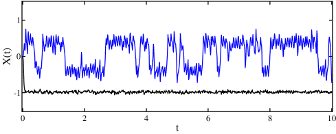
(c) Controlled and uncontrolled sample paths

Figure 2: Particle in a double-well potential. In (a), the potential (10) is shown. Panel (b) shows a plot of the computed optimal control policy, as a function of position $x$, for $t=0$ and $T=30$. Panel (c) compares the controlled (lighter, blue curve) and uncontrolled (darker, black curve) sample paths.

Models of this type are paradigms for physical systems with multiple metastable states, and calculating transition rates between metastable states (due to large deviations in the driving white noise process) are of interest in, e.g., in reaction rate theory. By extension, the heights of relevant potential barriers are also of interest. Our goal here is to estimate the barrier height $A$ in Eq. (10).

For this 1D model, it is straightforward to solve the optimal control problem. Specificially, we discretize the interval $(-5,5)$ (with high probability the position $x_{t}$ will stay within this range) by 100 grid points. The control values $u_{t}$ are drawn from the finite set $\{0,\pm 2,\pm 4,\cdots,\pm 10\}$. We also assume a uniform prior for $A$ on the interval $[2,5]$, which we discretize into 10 parameter values. The diffusion process (9) is discretized in time with a timestep of $\mbox{\small$\Delta$}{t}=0.01$; this is sufficiently small to satisfy the criteria set forth in Sect. A. An optimal control policy is computed over the time interval $t\in[0,T]$ for various values of $T$. The computed control for $t\ll T$ stabilize rather quickly as $T$ increases; the control at $t=0$ is shown in Fig. 2(b). Not surprisingly, the control encourages more frequent jumps by pushing left when the particle is in the right well, and vice versa.

To see the control policy “in action,” we carry out simulations of the controlled diffusion proceess for $T=4$ and for $T=30$. For each choice of $T$, we carry out 256 independent trials, and use the result to estimate the barrier height $A$. The diffusion process is observed every 0.25 units of time; at observation times the system state is estimated, and the control value updated. The observations are assumed to have additive, Gaussian observation noise of standard deviation 0.05. Because of the observation noise, even though this is a 1D model (and so the full state “vector” is observed), filtering is still needed. Here, we use a particle filter with $10,000$ particles; far fewer particles would have sufficed for the controlled process, but the uncontrolled process needed more particles to obtain a reasonable parameter estimate. A sample trajectory subjected to the optimal control is shown in Fig. 2(c) (lighter / blue curve).

Duration	Control	N	In range	Mean	Bias	Std. Dev.	Std. Dev. Err.
4	Dynamic	256	100%	4.233	0.3933	0.05947	0.002628
4	0	256	98%	4.242	0.4016	0.3133	0.01385
30	Dynamic	256	100%	4.225	0.3854	0.02098	9.272e-4
30	0	256	99.6%	4.223	0.3832	0.2888	0.01277

(a) Continuous noise-free observations

Duration	Control	N	In range	Mean	Bias	Std. Dev.	Std. Dev. Err
4	Dynamic	256	100%	4.225	0.3846	0.1094	0.004833
4	0	256	77%	4.202	0.3623	0.6048	0.02673
30	Dynamic	256	100%	4.197	0.357	0.04881	0.002157
30	0	256	71%	4.316	0.4763	0.5953	0.02631

(b) Infrequent, noisy observations

Table 1: Comparison of estimates of the energy barrier height in the double well potential example using controlled and uncontrolled diffusions. in-range = number of trials where estimator falls within uniform prior; bias = difference between the mean over tries and the true value; std. dev. = standard deviation of the estimator; and std. dev. err. = our estimate of the standard error of the standard deviation. Dynamic control shows a clear improvement in the precision of estimates.

Table 1 shows the results of these trials. In Table 1(a), results are shown for full observation trials, in which the system is observed at every timestep, i.e., observation period = $\mbox{\small$\Delta$}{t}=0.01$ . In addition to the controlled diffusion process, we also computed $A$ estimates for the diffusion process with a range of constant control values $u\in{\cal U}$, and found that $u=0$ gives minimum-variance estimates among the control values tested. As can be seen, the standard deviation of the estimate based on the controlled diffusion is significantly smaller for both $T=4$ and $T=30$ — for $T=4$ by a factor of $\approx 5,$ and for $T=30$ by a factor of $\approx 14.$ We note that there is a measurable bias in the estimates from both dynamic and constant control regimes. In practical experiments, this can be examined and corrected by conducting a simulation; we note that the dynamic control policy does not appear to affect the magnitude of this bias.

Table 1(b) shows the corresponding results for the case of noisy-and-infrequent observations. For $T=4$, we obtain a roughly factor of 6 reduction in standard deviation, while for $T=30$, roughly a factor of 11. The reduction in the estimator variance is significant, though as expected somewhat less than the full observation case, at least over longer timescales. More telling is the fraction of estimates that were “in-range” (see the discussion of MLE in Appendix B): the controlled diffusion process always produced estimates that were within the prior parameter range, whereas the uncontrolled diffusion produces a nontrivial number of parameter estimates outside the range.

The reason that the optimal control strategy is particularly effective in this model is that while the barrier height $A$ has a significant impact on the dynamics of the system over long timescales, it only impacts the dynamics in a small part of state space, and on shorter timescales it has relatively little effect. The optimal control policy is able to drive the system into crossing the barrier much more frequently, thereby yielding more information about $A$. Note in order to know which way to drive the system to speed up barrier-crossing, the controller needs to know which state the particle is in.

We expect that, in general, our method will be particularly effective in situations like this, where the information-rich region of phase space is relatively small (in terms of how much time the uncontrolled trajectory spends there), and the control is able to increase the frequency of visits to these regions.

5 Morris-Lecar (ML) Neuron Model

We now demonstrate the application of the optimal control methodology to a more complex model with different dynamics, with the goal of examining how the type of dynamics can affect the efficacy of parameter estimation in the presence of dynamic control. Appendix D presents a further exploration of a different system where our methods are less helpful. The Morris-Lecar (ML) neuron model mentioned in the introduction is often used to model membrane voltage oscillations and other properties of neuronal dynamics; it describes how membrane voltage and ion channels interact to generate electrical impulses, or “spikes,” which is the primary means for neuronal information transmission. The ML model is planar, and hence more amenable to analysis than higher-dimensional models like the Hodgkin-Huxley equations (Hodgkin and Huxley, 1952). At the same time, it faithfully captures certain important aspects of neuronal dynamics (Ermentrout and Rinzel, 1998), making it a commonly-used model in computational neuroscience. It has a rich bifurcation structure, and exhibits two dramatically different timescales. See Ermentrout and Terman (2010) and Ermentrout and Rinzel (1998) for a derivation and description of this model and its behavior.

The ML model is given by (2). To provide further details, the second equation can be interpreted as the master equation for a two-state Markov chain describing the opening and closing of ion channels. The terms with $\beta_{v}$ and $\beta_{w}\gamma(v,w)$ are independent noise terms modeling different sources of noise: the $\beta_{v}$ term models voltage fluctuations, and is simply additive white noise. The $\beta_{w}\gamma(v,w)$ term models random fluctuations in the number of open ion channels due to finite-size effects; here we use the function

$$\gamma(v,w)=\sqrt{\frac{\varphi}{\tau_{w}(v)}\Big{(}w_{\infty}(v)\cdot(1-2w)+w\Big{)}},$$ (11)

to scale the Wiener process. This function arises from an underlying Markov chain model; see, e.g., Kurtz (1971, 1981); Smith (2002).

Here, we assume a typical experimental set-up in which an electrode (a “dynamic clamp”) is attached to the neuron, through which an experimenter can inject a current $I_{t}$ and measure the resulting voltage $v_{t}$; the gating variable $w_{t}$ is not directly observable. The electrode is usually attached directly to a computer, which records the measured voltage trace and generates the time-dependent injected current, making this type of experiment a natural candidate for our method. Neuronal membrane voltages are measured with signal-to-noise ratios of 1000 to 1 or more. On the other hand, dynamical events of interest can take place on timescales of milliseconds or less. So for this application it is vital that one pre-computes as much as possible. These speed requirements may necessitate the use of computationally cheaper — but less accurate — state estimation technique, e.g., ensemble Kalman filters. Since we are interested evaluating the utility of dynamic control via simulations, we continue to use particle filters here.

We focus on a parameter regime in which the noiseless system can switch between having a globally-attracting fixed point and an unstable fixed point surrounded by a stable limit cycle (Fig. 3(a) illustrates the latter). The limit cycle represents a “tonically” (periodically) spiking neuron; the effect of noise is to “smear out” this limit cycle. The precise parameters we use come from Ermentrout and Terman (2010); they are summarized in Appendix C. The key parameter here is the injected DC current; in Fig. 3(a) this is $I\equiv 100.0$. As one decreases $I$ from this value, the system undergoes a subcritical Hopf bifurcation: the unstable fixed point becomes stable, and at the same time an unstable periodic orbit emerges around the fixed point (Ermentrout and Terman, 2010). Post-bifurcation, the system is bistable: while tonic spiking continues to be viable, a quiescent state (corresponding to the stable fixed point) has emerged. If we decrease $I$ even further, the stable and unstable cycles collide in a saddle-node bifurcation, leaving behind a single stable fixed point.

In this example, our control is $u_{t}=I_{t}/C_{m}.$ The control values we use are $u\in\{0,3.5,5\},$ corresponding to $I\in\{0,70,100\}$ (we take $C_{m}=20$). The three values of the injected current place the system in the stable fixed point, bistable, and limit cycle regimes, respectively.

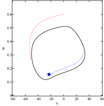
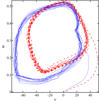
(a) Noiseless ML phase portrait	(b) Controlled and uncontrolled trajectories

Figure 3: Morris-Lecar (ML) phase portrait of a stimulated neuron. See (2). Time is measured in ms, voltage in mV, current in pA. In (a), the phase portrait of the noiseless ML system is shown. A stable limit cycle surrounds an unstable cycle, which in turn surrounds a sink. In (b), two trajectories for the noisy system are shown: the dotted curve is a trajectory without control, while the solid curve is a controlled trajectory.

Simulation results

We have performed simulations in which we estimated the calcium conductance constant $g_{Ca}$ from simulated data; this is chosen over other parameters because it gives rise to a more complex control policy (as we show below). In detail, we assume a flat prior for $g_{Ca}$ on the interval $[4,5]$; in all experiments reported below, we fix a randomly-generated $g_{Ca}$ value of 4.415, which we take to be the “true” value. The optimal control is computed using a timestep of $\approx 2$ ms, and we assume that measurements are available at every time step. State space is discretized by cutting the region $[-80,80]\times[0,1]$ into $72\times 72$ bins. Unless otherwise stated, “constant control” means $u_{t}\equiv 5$. The value of $u=5$ was chosen as the best performing among several possible values of a constant control, which all exhibited significantly higher standard deviations.

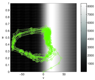
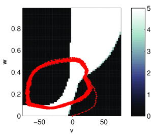
(a)	(b)

Figure 4: Control policy for parameter $g_{Ca}$ in the Morris-Lecar example (2). In (a), the FI is shown behind a single controlled trajectory. The lighter the region, the more informative that part of state space is about $g_{Ca}$. In (b), the control policy is depicted behind a single controlled trajectory. The control is adapted to the current state of the system in order to keep the trajectory in more informative regions.

Fig. 3(b) shows examples of controlled and uncontrolled (with $u=5$, or $I=100$) trajectories: the perturbations are measurable, but not large. Simulation results for estimates of $g_{Ca}$ using trajectories of duration $T=1000$ ms are given in Table 2.

Observation	Control	Mean	Bias	Std. Dev.
Full	Dynamic	4.416	6.315e-4	0.01106
Full	5.0	4.416	8.82e-4	0.01405
Noisy partial	Dynamic	4.413	-0.002062	0.01579
Noisy partial	5.0	4.416	0.001458	0.01847

Table 2: Simulation results for the Morris-Lecar example. “Full observation” runs use exact information from the entire state-space trajectory, while “Noisy partial” runs correspond to only observing $v_{t}$ corrupted by observational noise. Here, $T=1000$.

To better understand why the dynamic control performs better, we examine the structure of the control policy and Fisher information. Fig. 4(a) shows the Fisher information function for $g_{Ca}$, which is easily shown to be proportional to

$$\big{[}m_{\infty}(v_{t})~{}(v_{t}-E_{Ca})\big{]}^{2}~{};$$

the controlled trajectory is superposed. From the geometry, one expects the optimal control should either find a way to keep the trajectory at a constant voltage or, failing that, try to increase the firing rate, so that trajectories cross the information-rich region as much as possible. As can be seen, the controlled trajectory does exactly that: starting at the resting voltage (around -80 mV), it jumps toward 0 mV, runs along the “information-rich” strip around $v=20$ before dipping back toward the resting voltage. In comparison, the uncontrolled trajectory in Fig. 3(b) appears to spend less time in this region. Fig. 4(b) shows how the optimal control policy accomplishes this by suitably pushing the trajectory at critical parts of its cycle, thus increasing the overall firing rate.

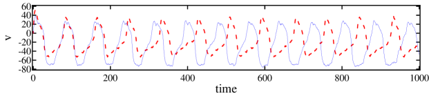
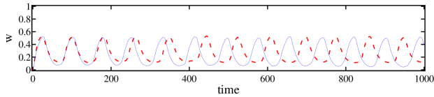
Figure 5: Trajectories of the Morris-Lecar model under constant control (dashed) and optimal control (solid). We see the optimal control has higher frequency oscillations which force the trajectories through the most informative state space more often.

To see more clearly the effect of the dynamic control, we plot time traces of the controlled and uncontrolled trajectories in Fig. 5. As can be seen, the dynamic control not only tries to push the trajectory into the information-rich region, it also makes sure it spends more time there.

Some final remarks on the structure of the optimal control:

1. We note that the optimal control depends a great deal on the parameter being estimated. If one were to try to estimate $C_{m}$, for example, the resulting control policy is essentially constant for most of phase space.

2. In this dynamic regime, with FI as in Fig. 4(a) (a unimodel function of $v$), it is natural to expect that increasing firing rate leads to an increase in the FI. This can be accomplished by either dynamic control or by static control. In more general situations, e.g., neuron models with additional currents and exhibiting dynamics on multiple timescales (Dayan et al., 2001), we expect dynamic control to yield a greater gain in FI. However, since such models usually entail $>3$ degrees of freedom, they would be difficult to study using present numerical methods, and we leave the study of such models for future work.

6 Discussion

There has been increasing interest in combining experimental data and statistical methods with mechanistic dynamical models describing system behavior. This paper adds to this literature in considering the problem of designing inputs into such experiments that are directed at improving the precision of parameter estimates that result from them. In particular, we have demonstrated that in diffusion processes, maximizing Fisher Information about a parameter can be cast as a problem of optimal control and shown that using this strategy can substantially improve parameter estimates. In order to make control methods feasible when systems are observed with noise or only some state variables are observable, we employ the strategy of estimating the value of the state on-line and using this within a pre-computed control policy.

We have demonstrated this approach on two examples that showcase when this form of adaptive control is most likely to be useful. One situation when we expect significant benefit from dynamic control is when visits to the information-rich regions of state space are relatively rare, as in the double-well example. As we have seen, optimal control can be effective in increasing the frequency of visits to information-rich regions. In systems where trajectories naturally return to information-rich regions in a recurrent fashion even with static controls, our method may still yield modest benefits, but the exact degree of information gain will depend on the specific dynamic situation.

In systems with stable fixed points that are already informative about the parameters of interest, dynamic control may not be better than simply choosing an optimal static control. However, our methods also yield information about which constant control is likely to be most useful; this is helpful in, e.g., the chemostat experiments described in Appendix D, where measurements are relatively infrequent and dynamic control is relatively easy to implement. In systems such as (8) in which the location of fixed points do not yield information about parameters, a control policy that repeatedly returns the system to informative transient states could be more advantageous.

There remain numerous unresolved problems and open areas in which these methods can be extended. Computational cost, both in speed and memory, represent the largest limiting factor in employing these methods. In particular, the storage and computation costs of the policy scale exponentially with the number of state variables. Possible strategies here involve the application of sparse grid strategies for discretizing the state variables (Xiu, 2009) or – more heuristically – intensive Monte Carlo methods to simulate the state variables forward combined with machine learning methods to estimate control strategies. It may also be possible to pre-compute control policies only for high-probability regions of the state space and employ techniques of approximate dynamic programming (Powell, 2007).

Further extensions involve alternative targets for the control policy, including the Bayesian criteria explored in Busetto et al. (2009). Thorbergsson and Hooker (2012) explores maximizing the Fisher Information for a partially observed Markov decision process, although this exacerbates the computational difficulties discussed above. Another direction for extension is to systems with vector parameters:our methods can be readily extended to maximizing the trace of a Fisher Information matrix ($T$-optimal designs); other criteria such as the determinant ($D$-optimality) that can be expressed as combinations of time integrals can also be employed using the same ideas.

We have dealt with parameter uncertainty before the experiment by averaging the Fisher Information over the prior within our objective. Alternative strategies such as maximizing the minimum Fisher Information in a range of parameters can be implemented within the numerical control strategy. We have also not experimented with updating our prior as the experiment progresses; this can be accomplished within particle filtering, for example by treating parameters as additional state variables – an approach taken in Ionides et al. (2006) – although when observations are highly informative about the system state, this can result in particle filter collapse (Snyder et al., 2008) (recent advances such as implicit filters (Chorin et al., 2012) may be helpful here).  Such an approach would also require either re-computing the optimal policy after each observation, or precomputing the control for a range of parameters and suitably combining them, but when the optimal control policy depends strongly on the system parameters such updates may be expected to produce significant improvements.

Acknowledgments.

We thank Prof. Cindy Greenwood for many helpful comments throughout the initial stages of this work, and Prof. Xueying Wang for help with the Morris-Lecar model. We are also grateful to the anonymous referees for numerous suggestions and relevant references. This work was supported in part by the Statistical and Applied Mathematical Sciences Institute (KL, BR), the National Science Foundation under grants DMS-1418775 (KL), DMS-1053252 and DEB-1353039 (GH).

Appendix A Markov chain approximation

This section provides technical details of our numerical methods for obtaining the optimal control policy. As noted above, in order to execute the dynamic programming strategy on a computer and tabluate the resulting control policy $F$, it is necessary to discretize the state space. Here we follow a discretization strategy due to Kushner (Kushner, 1971). The starting point is the time-$t$ distribution $\rho(t,\cdot)$ of the diffusion $\mbox{\bf x}_{t}$, which satisfies the forward equation

$$\partial_{t}\rho(t,\mbox{\bf x})+\sum_{i}\partial_{x_{i}}\big{(}\mbox{\bf f}(\mbox{\bf x},\theta,F(\mbox{\bf x},t))\rho(t,\mbox{\bf x})\big{)}=\frac{1}{2}\sum_{i,j}\partial_{x_{i}}\partial_{x_{j}}\big{(}\Sigma_{ij}(\mbox{\bf x})~{}\rho(t,\mbox{\bf x})\big{)}~{},$$ (12)

where $F$ is the optimal control plan described above in the limit $\mbox{\small$\Delta$}{t}\to 0~{}.$ We discretize the optimization problem (7) as follows: (i) we cover the relevant portions of state space with a finite grid of points with spacing $h$; (ii) we then discetize Eq. (12) in space and time by a finite difference approximation on this grid with a timestep $\mbox{\small$\Delta$}{t}^{h}$ depending on $h$; and (iii) we interpret the coefficients of the finite difference approximation as the transition probabilities of a finite-state Markov chain (whose states are the discrete grid points chosen in (i)) to approximate the diffusion process. The dynamic programming algorithm can then be applied directly to this finite state Markov chain in a straightforward manner.

As an example of what we mean by (iii), consider the simple diffusion equation $\partial_{t}u=\partial_{x}^{2}u$. The standard finite difference discretization of this PDE is

$$u(t+\mbox{\small$\Delta$}{t},x) =u(t,x)+\frac{\mbox{\small$\Delta$}{t}}{h^{2}}\big{(}u(t,x+h)+u(t,x-h)-2u(t,x)\big{)}$$

$$=(1-2\mu)u(t,x)+\mu(u(t,x+h)+u(t,x-h))~{},$$

where $\mu=\mbox{\small$\Delta$}{t}/h^{2}~{}.$ Thus, if $\mu\in(0,\nicefrac{{1}}{{2}})$, we can interpret the equation above as describing a discrete state-space Markov chain whose states are $\{0,\pm h,\pm 2h,\cdots\}$ with transition probability $P(X_{k+1}=x|X_{k}=x)=1-\mu$ and $P(X_{k+1}=x\pm 1|X_{k}=x)=\mu$ . Note that the condition $0<\mu<1$ imposes an upper bound on the stepsize, specifically $\mbox{\small$\Delta$}{t}\leq h^{2}/2$ . Timestep limitations like this are a general feature of finite difference discretization schemes, and a poorly-designed finite difference scheme can lead to a great increase in computational cost.

The main technical problem is thus step (ii), since we need to ensure that the coefficients of the finite difference scheme can be interpreted as probabilities. In our implementation, we employ a “split operator” finite difference discretization. Roughly speaking, this amounts to discretizing the drift and diffusion terms in the SDE (1) separately, then composing the resulting difference schemes. This is a standard technique often used for the numerical solution of partial differential equations (see, e.g., Strikwerda, 1989). In our test examples, the use of such a split operator scheme permits us to use larger grid spacings and timesteps while maintaining numerical stability, and can significantly speed up overall running speeds.

In detail: first, suppose for simplicity that the state space in Eq. (1) is ${\mathbb{R}}$ (generalization to higher dimensions is straightforward, but with more complex notation). For each $h>0$, let ${\cal G}_{h}$ denote the regular grid $h{\mathbb{Z}}$ with spacing $h$. For the moment, assume ${\cal G}_{h}$ extends to all of ${\mathbb{R}}$; boundary conditions are discussed below. The grid ${\cal G}_{h}$ will be the state space of our discrete-time approximating Markov chain $\tilde{\mbox{\bf x}}_{i}$. To choose time step sizes, we fix a constant $\mu>0$ and an integer $r>0$, and set the timestep to be $\mbox{\small$\Delta$}{t}^{h}=\mu h^{2}.$ Then our approximation can be described as follows:

Step 1. Suppose at time $t=i\mbox{\small$\Delta$}{t}^{h}$, the chain has state $\tilde{\mbox{\bf x}}_{i}=sh.$ Then

• with probability $|f(sh)|\cdot\mbox{\small$\Delta$}{t}^{h}/h$, jump to $(s+1)h$ if $f(sh)>0$ and to $(s-1)h$ if $f(sh)<0$; and

• stay at $sh$ with probability $1-|f(sh)|\cdot\mbox{\small$\Delta$}{t}^{h}/h.$

Step 2. Let $s^{\prime}h$ denote the state of the chain after the previous step. Then jump to $(s^{\prime}\pm r)h$ with probability $\tfrac{1}{2}\Sigma(s^{\prime}h)\mu/r^{2}$, and stay at $s^{\prime}h$ with probability $1-\Sigma(s^{\prime}h)\mu/r^{2}$.

This discretization scheme treats the drift and diffusion terms in Eq. (1) separately, hence the name “split operator.” It is straightforward to show that the composite finite difference discretization provides a consistent discretization of Eq. (12). Step 1 interprets the drift term as a biased jump, and Step 2 interprets the diffusion term as one step of a symmetric random walk.

Both conceptually and in terms of programming, split operator schemes like the one above are easy to work with; however they also impart an additional variance on the motion of the approximating Markov chain. In the scheme above, this extra variance is on the order of $O(h\mbox{\small$\Delta$}{t}^{h})=O(h^{3})$ per step; the relative effect of this extra variance (so-called numerical diffusion) vanishes as $h\to 0$.

Clearly, in order for the various expressions above to be valid transition probabilities, we must have $\mu/r^{2}<\inf_{x\in{\mathbb{R}}}\Sigma(x)^{-1}.$ We also need $\sup_{x}|f(x)|\mbox{\small$\Delta$}{t}^{h}/h<1$. Since $\mbox{\small$\Delta$}{t}^{h}/h=\mu h$, the second condition can always be achieved by taking $h$ sufficiently small. The first condition, however, places a rather stringent constraint on the timestep $\mbox{\small$\Delta$}{t}^{h}.$ The purpose of introducing the “skip factor” $r$ is precisely to partially alleviate this constraint, at the cost of losing some accuracy. In practice, going from $r=1$ to $r=2$ can have a large impact on the overall running time. If $r=1$, our scheme closely resembles the “up-wind” scheme of Kushner (Kushner, 1971); a scheme similar to our $r=2$ case is also described there.

In practice, rather than choosing $h$ and $\mu$, we usually first choose $h$ and $\mbox{\small$\Delta$}{t}$, and take $r\propto\Sigma_{max}\sqrt{\mu}$ with a constant of proportionality between 1 and 2, where $\Sigma_{max}$ is the maximum of $\Sigma(x)$ over the domain of interest. This guarantees that the scheme converges (see below). We usually use relatively coarse grids, as (i) the structure of the optimal control policy is not too fine, and (ii) we usually operate in the presence of observation and dynamical noise, so there is not much point trying to pin down fine structures in the control policy.

Convergence. In general, a sufficient condition for the Markov chain approximation method to be valid is that the approximating chain $\tilde{\mbox{\bf x}}_{i}$ satisfy

$$E_{i}(\tilde{\mbox{\bf x}}_{i+1}-\tilde{\mbox{\bf x}}_{i}) =\mbox{\bf f}(\tilde{\mbox{\bf x}}_{i},u_{i})\mbox{\small$\Delta$}{t}+O(h^{\alpha}\mbox{\small$\Delta$}{t})$$

$$\mbox{Var}_{i}(\tilde{\mbox{\bf x}}_{i+1}-\tilde{\mbox{\bf x}}_{i}) =\Sigma(\tilde{\mbox{\bf x}}_{i})\mbox{\small$\Delta$}{t}+O(h^{\alpha}\mbox{\small$\Delta$}{t})$$

$$|\tilde{\mbox{\bf x}}_{i+1}-\tilde{\mbox{\bf x}}_{i}| =O(h)$$

(Kushner, 1971). In the above, $E_{i}(\cdot)$ denotes conditional expectation given all information up to step $i$, $\mbox{Var}_{i}(\cdot)$ denotes the corresponding autocovariance matrix, and $\alpha>0$ is a constant. Note the last line should be interpreted to hold surely, i.e., it says the discrete Markov chain makes jumps of $O(h)$ in size. If the conditions above are satisfied, then as $h\to 0$, the optimal control policy for the approximating chain will converge to an optimal control policy for the diffusion (1). It is easy to see that our scheme satisfies the convergence criteria above with $\alpha=1.$

Boundary conditions. In practice, ${\cal G}_{h}$ must be a finite grid. We assume that it spans a subset of ${\mathbb{R}}^{d}$ sufficiently large that on the timescale of interest, trajectories have very low probability of exiting. We then impose that when the approximating Markov chain attempts to exit the domain, it is forced to stay at its current state. This gives a simple way to obtain a Markov chain on bounded grids.

Higher dimensions. The generalization of the preceding scheme to higher dimensions is straightforward: we simply treat each dimension separately and independently.

Appendix B Numerical Methods for Particle Filters and Maximum Likelihood Estimation

In this appendix we provide details of our particle filter methods to estimate both the state value given current observations and for maximum likelihood estimation. We discretize the diffusion process using the standard Euler-Maruyama approximation (4), and incorporate observations via Bayes’s formula. In all the examples considered in this paper, the observations are linear functions of the state vector plus Gaussian error. This allows us to avoid weighting and resampling in the particle filter. Instead, we incorporate the observations within the Euler-Maruyama scheme (4) by first applying the drift $\mbox{\bf f}(\mbox{\bf X}_{i},\theta,u_{i})~{}\mbox{\small$\Delta$}{t}$ and then sampling the Gaussian disturbance $\sqrt{\mbox{\small$\Delta$}{t}}~{}\Sigma^{1/2}(\mbox{\bf X}_{i})\mbox{\boldmath${\epsilon}$}_{i}$ conditional on the observation at time $i+1$. When multiple steps are taken between observations, this update is applied for the final step. In practical terms, our particle filters are simpler and more robust than bootstrap filters, and do not differ significantly from other popular filtering schemes, e.g., the ensemble Kalman filter.

One additional implementation detail: when observations are infrequent, we simply hold the control value constant between observations. In principle, we can also use the past information to extrapolate the state trajectory between observations, and use a time-dependent control. But for the examples considered in this paper, the simpler strategy appears sufficient; it is also more realistically applicable in some experiments.

Maximum likelihood estimates

Another advantage of using particle filters is that we can easily evaluate the likelihood as a bi-product. Let $I$ be the relevant parameter interval (see Sect. 2.2), and for simplicity assume a flat prior over $I$. We discretize $I$ into a discrete grid $I_{M}$ of size $M$. For each putative parameter value in $I_{M},$ we run a particle filter and compute an estimate of the log-likelihood using the formula (Ionides et al., 2006)

$$\mbox{log likelihood}=\sum_{k=0}^{n}\log\big{(}p(\mbox{\bf y}_{k}|\mbox{\bf y}_{1},\cdots,\mbox{\bf y}_{k-1})\big{)}\approx\sum_{k=0}^{n}\log\left(\frac{1}{N}\sum_{i=1}^{N}p\big{(}\mbox{\bf y}_{k}\big{|}\mbox{\bf x}^{(i)}_{k}\big{)}\right)$$

where $\{\mbox{\bf x}^{(i)}_{k}:i=1,\cdots,N\}$ denotes the ensemble of particles at step $k$. If the computed log-likelihood curve takes on a maximum in the interior of the interval $I,$ we do a standard 3-point quadratic interpolation around the maximum and find the maximizer; we use this as the MLE. On the rare occasions when the log-likelihood curve does not have a maximum inside the interval $I,$ we use the corresponding endpoint as the estimate (but record the estimate as being “out of range”).

One further “trick” can be used to improve the performance of the grid-based MLE: for each simulation experiment, corresponding “particles” for different parameter values are driven using the same sequences of Gaussian random numbers. That is, if the $i$th particle in the ensemble for the $j$th parameter value is in state $\mbox{\bf x}^{i,j}_{k}$ at timestep $k$, then the particle positions $\mbox{\bf x}^{i,1}_{k+1},\cdots,\mbox{\bf x}^{i,M}_{k+1}$ at the next timestep (where $M=$ number of points in the parameter grid) are generated from the current positions $\mbox{\bf x}^{i,1}_{k},\cdots,\mbox{\bf x}^{i,M}_{k}$ using the same Gaussian random numbers. (To ensure correct sampling, the particles $\mbox{\bf x}^{1,j}_{t},\cdots,\mbox{\bf x}^{N,j}_{t}$ for fixed $j$ still receive independent Gaussian random numbers.) This same-noise coupling or method of same paths reduces the variance of the resulting estimates (Asmussen and Glynn, 2008), and produces smooth likelihood curves.

For comparison purposes, we also study the full observation problem in some of the examples, i.e., assume the full state vector is continuously and noiselessly observed. For such problems, the log-likelihood associated with particular sample paths are straightforward to calculate directly, and filtering is not needed.

Appendix C ML Model Parameters

Here we briefly summarize the details of the ML model used in this paper. The interested reader is referred to (Ermentrout and Rinzel, 1998; Ermentrout and Terman, 2010) for more details.

Recall the (deterministic) ML equations

$$\begin{array}[]{rl}C_{m}\dot{v}&=I(t)-g_{\rm leak}\cdot(v-E_{\rm leak})-g_{K}~{}w\cdot(v-E_{K})-g_{\rm Ca}~{}m_{\infty}(v)\cdot(v-E_{\rm Ca})\\[8.61108pt] \dot{w}&=\phi\cdot\big{(}w_{\infty}(v)-w\big{)}/\tau_{w}(v)\end{array}$$

As explained in Sect. 5, the ML model tracks the membrane voltage $v$ and a gating variable $w$. The constant $C_{m}$ is the membrane capacitance, $\phi$ a timescale parameter, and $I(t)$ an injected current. The reversal potentials $E_{\{K,Ca,leak\}}$ and associated conductances $g_{\{K,Ca,leak\}}$ characterize the ion channels and their dependence on the membrane voltage (see below).

Spike generation depends crucially on the presence of voltage-sensitive ion channels that are permeable only to specific types of ions. The ML equations include just two ionic currents, here denoted calcium and potassium. The voltage response of ion channels is governed by the $w$-equation and the auxiliary functions $w_{\infty}$, $\tau_{w}$, and $m_{\infty}$, which have the form

$$\begin{array}[]{rcl}m_{\infty}(v)&=&\frac{1}{2}\big{[}1+\tanh\big{(}(v-v_{1})/v_{2}\big{)}\big{]},\\[6.45831pt] \tau_{w}(v)&=&1/\cosh\big{(}(v-v_{3})/(2v_{4})\big{)},\\[6.45831pt] w_{\infty}(v)&=&\frac{1}{2}\big{[}1+\tanh\big{(}(v-v_{3})/v_{4}\big{)}\big{]}.\end{array}$$

The function $m_{\infty}(v)$ models the action of the relatively fast calcium ion channels; $v_{\rm Ca}$ is the “reversal” (bias) potential for the calcium current and $g_{\rm Ca}$ the corresponding conductance. The gating variable $w$ and the functions $\tau_{w}(v)$ and $w_{\infty}(v)$ model the dynamics of slower-acting potassium channels, with its own reversal potential $v_{\rm K}$ and conductance $g_{\rm K}$. The constants $v_{\rm leak}$ and $g_{\rm leak}$ characterize the “leakage” current that is present even when the neuron is in a “quiescent” state. The forms of $m_{\infty}$, $\tau_{w}$, and $w_{\infty}$ (as well as the values of the $v_{i}$) can be obtained by fitting data, or reduction from more biophysically-faithful models of Hodgkin-Huxley type (see, e.g., (Ermentrout and Terman, 2010)).

The precise parameter values used in this paper are summarized in Table 3. These are obtained from (Ermentrout and Terman, 2010). Throughout, the noise intensities are $\beta_{v}=1$, $\beta_{w}=0.1$.

Parameter	Value
$I_{0}$	95
$C_{m}$	20.0
$g_{\rm Ca}$	4.41498308(∗)
$g_{K}$	8.0
$g_{\rm leak}$	2.0
$\phi$	0.04

Parameter	Value
$v_{K}$	-84.0
$v_{\rm leak}$	-60.0
$v_{\rm Ca}$	120.0
$v_{1}$	-1.2
$v_{2}$	18.0
$v_{3}$	2.0
$v_{4}$	30.0

Table 3: Parameter values used for the Morris-Lecar example. (*) The “target” value of $g_{Ca}$ is randomly generated from a certain range.

Appendix D Chemostat Growth Models

Our second example comes from experimental ecology. In these experiments, a glass tank or chemostat is inoculated with a population of algae. The tank is bubbled to ensure that the contents are mixed, and to prevent oxygen deprivation. A nitrogen-rich medium is continuously injected while the contents of the tank are evacuated at the same rate as the injection. Algae are assumed to consume nitrogen in proportion to their population size and nitrogen concentration, until the population size stabilizes due to saturation. For ecological models a set of stochastic differential equations can be proposed with drift term

$$dN_{t} =\left(\delta(t)\eta_{I}(t)-\frac{\rho C_{t}N_{t}}{\kappa+N_{t}}-\delta(t)N_{t}\right)dt$$ (13)

$$dC_{t} =\left(\frac{\chi\rho C_{t}N_{T}}{\kappa+N_{t}}-\delta(t)C\right)dt$$

where the model has a mechanistic interpretation for an infinite population given in terms of:

$N_{t}$

($\mu$ mol/l) represents the nitrogen concentration in the chemostat

$C_{t}$

($10^{9}$ cells per liter) gives the relative algal density

$\delta(t)$

(percentage per day) is the dilution rate; i.e., the rate at which medium is injected and the chemostat evacuated

$\eta_{I}(t)$

($\mu$ mol/l) is the nitrogen concentration in medium

$\rho$

($\mu$ mol/$10^{9}$ cells) is the rate of algal consumption of nitrogen

$\kappa$

($\mu$ mol/l) is a half-saturation constant indicating the value of $N$ at which $N/(\kappa+N)$ is half-way to its asymptote

$\chi$

($10^{9}$ cells/$\mu$ mol) is the algal conversion rate; how fast algae turn consumed nitrogen into new algae.

This system is made stochastic by multiplicative log-normal noise. This is equivalent to a diffusion process on $N^{*}_{t}=\log(N_{t})$ and $C^{*}_{t}=\log(C_{t})$ with additive noise:

$$dN^{*}_{t} =\left(\delta(t)\eta_{I}(t)-\frac{\rho e^{C^{*}_{t}+N^{*}_{t}}}{\kappa+e^{N^{*}_{t}}}-\delta(t)e^{N^{*}_{t}}\right)e^{-N^{*}_{t}}dt+\sigma_{1}dW_{1}$$

$$dC^{*}_{t} =\left(\frac{\chi\rho e^{C^{*}_{t}+N^{*}_{t}}}{\kappa+e^{N^{*}_{t}}}-\delta(t)e^{C^{*}_{t}}\right)e^{-C^{*}_{t}}dt+\sigma_{2}dW_{2}.$$

Here, the diffusion terms provide an approximation to stochastic variation for large but finite populations and account for other sources of extra-demographic variation. While alternative parametrizations of stochastic evolution can be employed, the diffusion approximation is convenient for our purposes. A typical goal is to estimate the algal conversion rate $\chi$ and the half-saturation constant $\kappa$.

This experiment involves several experimental parameters that can be used as the dynamic input:

• The dilution rate of the chemostat $\delta(t)$

• The concentration of nitrogen input $\eta_{I}(t)$

• The times at which the samples are taken from the chemostat

• The quantities that are observed.

In this paper we use $\delta(t)$ as the control parameter, which fits well within the design methodology outlined above. Realistic values for the parameters, estimated from previous experiments, are $(\eta_{I},\rho,\chi,\kappa)=(160,270,0.0027,4.4)$. We chose $\sigma_{1}=\sigma_{2}=0.1$ based on visual agreement with past experiments; since these act multiplicatively on the dynamics it is reasonable for them to be of the same order of magnitude. We hold $\eta_{I}(t)$ constant; within the experimental apparatus, $\eta_{I}(t)$ can only be modified by changing between discrete sources of medium. Chemostats are typically inoculated with a small number of algal cells and the models above give algal density relative to a total population carrying capacity in the tens of millions. Under these circumstances, initial conditions can be given by $N^{*}_{0}=\log\eta_{I}$ (the input concentration) and $C^{*}_{0}\propto\log 10^{-5}$ representing an initial population of a few hundred cells. The experimental apparatus places further constraints on the problem: the dilution rate must be positive, and cannot exceed the maximal rate at which medium can be pumped through the chemostat.

We focus on the estimation of $\kappa.$ In this model system, one can measure both $C_{t}$ and $N_{t}$, though nitrogen measurements are both more costly to make and prone to distortion by various factors. Continuous measurements are not practical for either quantity; one can at best make measurements a few times a day. Here, we focus mainly on the complete-but-infrequenth observation regime, where we assume we can make (noisy) measurements of both state variables.

This system represents a most-marginal case for adaptive designs in that the system has a stable fixed point for each dilution rate and most information is gained near the fixed point. Further, the value of $\kappa$ mostly affects the fixed point of $N_{t}$. We thus expect that adaptive controls will exhibit little improvement over the best choice of a constant control policy and that estimates based solely on $C_{t}$ – by far the easier quantity to measure – will have poor statistical properties whatever policy is used. Figure 6 shows an example trajectory of this model along with the fixed point as a function of $\kappa$.

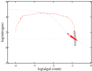
Figure 6: State space plot of the chemostat model. The solid curve is a single trajectory for the uncontrolled system. The horizontal dashed lines are the nullclines of the noise-free system. The thick gray line shows the movement of the fixed point as $\kappa$ varies from 2 to 12. Here, $\delta=0.3$ and $\kappa=4.4~{}.$

Model properties and further parameter constraints

We begin by examining the dynamic properties of the chemostat system. In the absence of noise, i.e., when $\sigma_{1}=\sigma_{2}=0~{}$, the phase space is fairly simple: it has a single fixed point given by

$$N^{*}_{0}=\log\Big{(}\frac{\kappa\delta}{\chi\rho-\delta}\Big{)},~{}~{}~{}~{}C^{*}_{0}=\log\Big{(}\frac{\delta(\eta_{I}-e^{N^{*}_{0}})(\kappa+e^{N^{*}_{0}})}{\rho e^{N^{*}_{0}}}\Big{)}.$$ (14)

It is easy to check that this fixed point is linearly stable, and attracts all initial conditions in the relevant part of state space. When $\sigma_{1},\sigma_{2}>0,$ all trajectories eventually converge to a neighborhood of the fixed point, and the stationary distribution is concentrated around the fixed point for moderate $\sigma_{1}$, $\sigma_{2}$. See Fig. 6. The fixed point exists only if the dilution rate $\delta$ is not too high; when $\delta>\delta_{c}$ for some critical $\delta_{c},$ the fixed point $(C_{0}^{*},N_{0}^{*})$ moves to $-\infty.$ Physically, this means the dilution rate is so high that the algal population crashes to 0. For $\kappa\approx 4$ (the typical value we assume in this example), the critical $\delta_{c}$ is roughly $0.7.$ To avoid crashing populations, we keep the dilution rate below this number.

As mentioned above, $C^{*}_{t}$ is easier to measure experimentally because it can potentially be done by an optical particle counter. Unfortunately, in the parameter regime of interest, it is actually fairly difficult to infer $\kappa$ from $C^{*}_{t}$ measurements alone. To see this, observe that for $\delta\in[0.1,0.6]$ and as $\kappa$ varies over $[2,12],$ the fixed point moves essentially vertically; see Fig. 6. Since trajectories are expected to stay near the fixed point, it follows that changing $\kappa$ will have a significant, observable impact on the $N^{*}_{t}$ dynamics but relatively little on $C^{*}_{t}.$ Equivalently, because our estimation strategy is based on the likelihoods of state variable observations, $N^{*}_{t}$ measurements (or combined $(C^{*}_{t},N^{*}_{t})$ measurements) will be much more useful for estimating $\kappa$ than $C^{*}_{t}$ alone. This is our reason for focusing on the complete-observation case.

Finally, we note that the FI for $\kappa$ is given by

$$\left|\left|\frac{d}{d\theta}\mbox{\bf f}(\mbox{\bf x}_{t},\theta,u_{t})\right|\right|^{2}_{\Sigma(\mbox{\bf x}_{t})}=\frac{\left(\frac{1}{\sigma^{2}_{1}}+\frac{\chi^{2}}{\sigma^{2}_{2}}\right)\rho^{2}C_{t}^{2}N_{t}^{2}}{\left(\kappa+N_{t}\right)^{4}}$$

which is maximized when $N_{t}=\kappa$ but for $C_{t}\rightarrow\infty~{}.$ As discussed in Sect. 2.2, if we allowed unbounded control values, a penalization would need to be imposed in order to avoid unrealistically large diluation rates. Since we are choosing dilution rates from a finite set here, this is not necessary. Figure 7 presents the control policy at times $T$ = 4, 7 and 30.

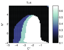
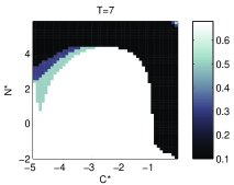
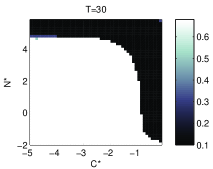
(a) $T=4$	(b) $T=7$	(c) $T=30$

Figure 7: Optimal control policies for the chemostat model. In (a-c), we show the optimal control policies for different durations $T$.

Simulation results

We now examine the effectiveness of the optimal control methodology via simulations of the chemostat model. We start at $(C^{*}_{0},N^{*}_{0})=(-4,2)$, corresponding to typical experimental conditions. With this initial condition, it typically takes a trajectory about 7 days or so (physical time) to reach equilibrium. In our simulations, we carry out experiments of duration $T$ for various values of $T$, ranging from 4 to 30 days. All simulation results are based on 256 realizations of the (controlled) diffusion process.

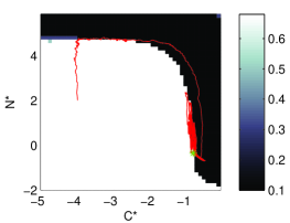
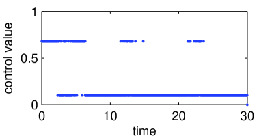
(a) A controlled trajectory	(b) The control $u_{t}$
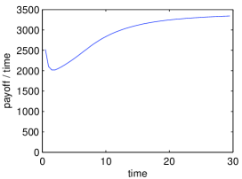
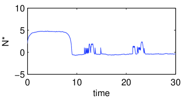
(c) Payoff / $T$ versus $T$	(d) The controled $N^{*}_{t}$

Figure 8: (a) Controlled trajectories of the chemostat system (13) along with the control used (panel b) and the resulting $N^{*}_{t}$ (d). Panel (c) shows $\overline{FI}(T)/T$, where $\overline{FI}(T)$ is the mean “pay-off,” i.e., Fisher information averaged over initial conditions and experimental realizations.

The optimal control policies, for different values of $T$, are shown in Fig. 7. The control values are drawn from the set $\{0.1,0.3,0.5,0.68\}$ (remaining below the dilution rate at which all the algae is eventually removed from the system), and we assume a flat prior for $\kappa$ over the interval $[3.5,5.5].$ As can be seen, the computed control policy is nontrivial and depends on $T.$ However, we observed that after about $T\approx 10$, the control policy stops changing. The “long-time,” steady-state control policy uses only the extreme values 0.1 and 0.68; on shorter timescales, the control policy uses all available values.

Fig. 8(c) shows the quantity $\overline{FI}(T)/T$, where $\overline{FI}(T)$ is the mean Fisher information (averaged over experimental realizations and initial conditions) as a function of duration $T.$ As can be seen, by $T=30$, the system has begun to approach the asymptotic regime, in which we expect $\overline{FI}(T)\propto T.$ To illustrate the effects of the optimal control, a controlled trajectory is shown in Fig. 8(a). The corresponding control values are shown in Fig. 8(b), as is the corresponding values of $N^{*}_{t}$ in Fig. 8(d) (not much of interest happens to $C^{*}_{t}$).

T	Control	N	In-range	Mean	Bias	Std. Dev.	Std. Dev. Err
4	Dynamic	256	54%	4.555	0.1551	0.7837	0.03464
4	0.1	256	62%	4.658	0.2577	0.7157	0.03163
4	0.3	256	26%	4.514	0.1137	0.9043	0.03996
4	0.68	256	16%	4.624	0.2243	0.938	0.04145
7	Dynamic	256	100%	4.402	0.002351	0.0395	0.001746
7	0.1	256	100%	4.399	-0.001245	0.04593	0.00203
7	0.3	256	35%	4.679	0.2788	0.8459	0.03738
7	0.68	256	18%	4.463	0.06275	0.9384	0.04147
15	Dynamic	256	100%	4.402	0.001752	0.00955	4.221e-4
15	0.1	256	100%	4.403	0.002518	0.01284	5.674e-4
15	0.3	256	100%	4.399	-8.251e-4	0.01969	8.704e-4
15	0.68	256	19%	4.446	0.04579	0.9314	0.04116
30	Dynamic	256	100%	4.402	0.001827	0.004443	1.964e-4
30	0.1	256	100%	4.402	0.001629	0.005766	2.548e-4
30	0.3	256	100%	4.403	0.002547	0.01075	4.752e-4
30	0.68	256	21%	4.532	0.1324	0.9216	0.04073

Table 4: Full observation results for the chemostat model. We perform $N$ independent trials for each experimental set-up. in-range = number of trials where estimator falls within uniform prior; bias = difference between the mean over tries and the true value; std. dev. = standard deviation of the estimator; and std. dev. err. = our estimate of the standard error of the standard deviation.

To assess the quality of $\kappa$ estimates, we estimated the variance of of the MLE, $\hat{\kappa}$ in simulations. Table 4 shows the results these. As can be seen, on shorter timescales, dynamic and constant controls do not differ much in terms of performance. But, on longer timescales (e.g., $T=30$), the optimal control performs significantly better than most constant control values, with the exception of $\delta=0.1$: with $\delta=0.1$, the constant-control system achieves close to the performance of the dynamic control. The reason for this is that given enough time, trajectories in this system all converge to the stable fixed point. At and near this fixed point, the optimal policy sets $\delta=0.1$, so once the trajectory is close to the fixed point, the optimal policy is largely indistinguishable from the constant policy. In principle, the dynamic control can offer a potential gain in information on shorter timescales (during the transient phase of the dynamics). But in this particular system, the dilution rate $\delta(t)$ has little effect on the dynamics during the transient, and controlled and uncontrolled dynamics do not differ much.

Noisy and Partial Observation Simulation

In Table 5, we turn our attention to complete-but-infrequent observation runs. Here, we observe the system twice a day (i.e., at intervals of $\Delta{t}=0.5$). Observation noise is $(0.025,0.025)$. Naturally, all the standard deviations are larger than the full observation case. The overall trends observed for full observations persist, and for the same reasons.

T	Control	N	In-range	Mean	Bias	Std. Dev.	Std. Dev. Err.
4	Dynamic	256	41%	4.64	0.2398	0.8295	0.03666
4	0.1	256	49%	4.57	0.1696	0.7967	0.03521
4	0.3	256	22%	4.502	0.1024	0.9191	0.04062
4	0.68	256	18%	4.461	0.06094	0.9385	0.04148
7	Dynamic	256	100%	4.415	0.01506	0.1332	0.005888
7	0.1	256	100%	4.398	-0.002385	0.1416	0.006259
7	0.3	256	30%	4.619	0.2187	0.8772	0.03877
7	0.68	256	12%	4.463	0.06347	0.9587	0.04237
15	Dynamic	256	100%	4.398	-0.001966	0.06015	0.002658
15	0.1	256	100%	4.4	-1.926e-4	0.05113	0.00226
15	0.3	256	100%	4.406	0.005561	0.08012	0.003541
15	0.68	256	20%	4.518	0.1175	0.9288	0.04105
30	Dynamic	256	100%	4.4	2.777e-4	0.03385	0.001496
30	0.1	256	100%	4.399	-6.979e-4	0.03149	0.001392
30	0.3	256	100%	4.406	0.005991	0.04461	0.001972
30	0.68	256	25%	4.446	0.04572	0.9107	0.04025

Table 5: Complete but infrequent observation results for the chemostat model. See Table 4 for key.

T	Control	N	In-range	Mean	Bias	Std. Dev.	Std. Dev. Err.
4	Dynamic	256	79%	8.493	0.09294	2.902	0.1283
4	0.1	256	78%	8.51	0.1103	2.608	0.1153
4	0.3	256	58%	8.419	0.01897	3.481	0.1538
4	0.5	256	54%	7.952	-0.4482	3.858	0.1705
4	0.7	256	58%	7.512	-0.8882	3.798	0.1678
7	Dynamic	256	72%	8.31	-0.0896	3.175	0.1403
7	0.1	256	84%	8.383	-0.01698	2.522	0.1114
7	0.3	256	70%	8.216	-0.1837	3.116	0.1377
7	0.5	256	62%	7.922	-0.4783	3.483	0.1539
7	0.7	256	55%	8.155	-0.2448	3.707	0.1638
15	Dynamic	256	73%	7.787	-0.6127	3.288	0.1453
15	0.1	256	88%	8.168	-0.2324	2.428	0.1073
15	0.3	256	78%	8.042	-0.3575	2.999	0.1325
15	0.5	256	74%	8.144	-0.2559	3.143	0.1389
15	0.7	256	65%	8.143	-0.2572	3.494	0.1544
30	Dynamic	256	84%	8.146	-0.2544	2.678	0.1183
30	0.1	256	82%	8.277	-0.1228	2.632	0.1163
30	0.3	256	77%	8.281	-0.1193	3.006	0.1328
30	0.5	256	90%	7.933	-0.4665	2.466	0.109
30	0.7	256	77%	8.154	-0.2457	3.045	0.1346

Table 6: Partial observation results.

Finally, to confirm our intuition, we show the results of partial observation runs in Table 6, where we observe only $C^{*}_{t}.$ As expected, we cannot estimate $\kappa$ very well at all: many of the estimates fall outside the prior range. Nevertheless, if we measure the estimator performance by the number of estimates that fall inside the prior range, we see that the controlled system is comparable to the best constant control. In order to accommodate the larger variance, we enlarge the prior range to $[2,12]$ in this set of simulations, and also set $\kappa=8.4$. This prior range is used both to calculate the control policy and to obtain maximum likelihood estimates as described in Sect. 3.1; since we cap the estimates to the extremes of the prior range when the MLE falls outside the range, this choice affects the estimator variance reported here. We note that as for any experimental design problem, in experimental situations the prior must be determined beforehand and obtaining an MLE outside the prior range is a good indicator that the prior was poorly chosen or the data are uninformative about the parameter.

References

- Aït-Shahalia (2008) Aït-Shahalia, Y. (2008). Closed-form likelihood expansions for multivariate diffusions. Annals of Statistics 36(2), 906–937.
- Andrieu et al. (2003) Andrieu, C., A. Doucet, S. S. Singh, and V. B. Tadić (2003). Proceedings of the IEEE 92, 423 – 438.
- Asmussen and Glynn (2008) Asmussen, S. and P. W. Glynn (2008). Stochastic Simulation: Algorithms and Analysis. Springer.
- Bartroff and Lai (2010) Bartroff, J. and T. L. Lai (2010). Approximate dynamic programming and its applications to the design of pahse 1 cancer trials. Statistical Science 25, 245–257.
- Bauer et al. (2000) Bauer, I., H. G. Bock, S. Körkel, and J. P. Schlöder (2000). Numerical methods for optimum experimental design in DAE systems. Journal of Computational and Applied Mathematics 120, 1–25.
- Bensoussan (1992) Bensoussan, A. (1992). Stochastic Control of Partially Observable Systems. Cambridge, UK: Cambridge University Press.
- Berger (1994) Berger, M. P. F. (1994). D-optimal sequential sampling designs for item response theory models. Journal of Educational Statistics 19(1), pp. 43–56.
- Botchu and Ungarala (2007) Botchu, S. K. and S. Ungarala (2007). Nonlinear model predictive control based on sequential monte carlo state estimation. In 8th International IFAC Symposium on Dynamics and Control of Process Systems.
- Brunel (2008) Brunel, N. (2008). Parameter estimation of ODEs via nonparametric estimators. Electronic Journal of Statistics 2, 1242–1267.
- Busetto et al. (2009) Busetto, A. G., C. S. Ong, and J. M. Buhmann (2009). Optimized expected information gain for nonlinear dynamical systems. In Proceedings of the 26th Annual International Conference on Machine Learning, ICML ’09, New York, NY, USA, pp. 97–104. ACM.
- Chaloner and Larntz (1989) Chaloner, K. and K. Larntz (1989). Optimal bayesian design applied to logistic regression experiments. Journal of Statistical Planning and Inference 21, 191–208.
- Chaloner and Verdinelli (1995) Chaloner, K. and I. Verdinelli (1995). Bayesian dexperimental design: A review. Statistical Science 10(3), 273–304.
- Chaudhuri and Mykland (1993) Chaudhuri, P. and P. A. Mykland (1993). Nonlinear experiments: Optimal design and inference based on likelihood. Journal of the American Statistical Association 88(422), 538–546.
- Chorin et al. (2012) Chorin, A., M. Morzfeld, X. Tu, and E. Atkins (2012). A random map implementation of implicit filters. Journal of Computational Physics 231, 2049–2066.
- Dayan et al. (2001) Dayan, P., L. F. Abbott, and L. Abbott (2001). Theoretical neuroscience: Computational and mathematical modeling of neural systems.
- Ermentrout and Rinzel (1998) Ermentrout, G. B. and J. Rinzel (1998). Analysis of neural excitability and oscillations. In C. Koch and I. Segev (Eds.), Methods of Computational Neuroscience, pp. 251–292. Bradford.
- Ermentrout and Terman (2010) Ermentrout, G. B. and D. Terman (2010). Foundations of Mathematical Neuroscience. Springer.
- Freidlin and Wentzell (2012) Freidlin, M. I. and A. D. Wentzell (2012). Random perturbations of dynamical systems, Volume 260. Springer.
- Girolami et al. (2010) Girolami, M., B. Calderhead, and S. A. Chin (2010). Riemannian manifold Hamiltonian Monte Carlo. Journal of the Royal Statistical Society in press.
- Hänggi et al. (1990) Hänggi, P., P. Talkner, and M. Borkovec (1990). Reaction-rate theory: fifty years after kramers. Reviews of Modern Physics 62(2), 251.
- Hodgkin and Huxley (1952) Hodgkin, A. L. and A. F. Huxley (1952). A quantitative description of membrane current and its application to conduction and excitation in nerve. J. Physiol. 133, 444–479.
- Hooker (2009) Hooker, G. (2009). Forcing function diagnostics for nonlinear dynamics. Biometrics 65, 613–620.
- Hooker and Ellner (2013) Hooker, G. and S. P. Ellner (2013). Goodness of fit and nonlinear dynamics: Mis-specified rates or mis-specified states? under review.
- Huang and Wu (2006) Huang, Y. and H. Wu (2006). Bayesian experimental design for long-term longitudinal hiv dynamic studies. Journal of Statistical Planning and Inference 138, 105–113.
- Huggins and Paninski (2011) Huggins, J. H. and L. Paninski (2011). Optimal experimental design for sampling voltage on dendritic trees in the low-SNR regime. Journal of Computational Neuroscience, to appear.
- Ionides et al. (2006) Ionides, E. L., C. Bretó, and A. A. King (2006). Inference for nonlinear dynamical systems. Proceedings of the National Academy of Sciences.
- Kilicaslan and Banks (2009) Kilicaslan, S. and S. P. Banks (2009). A separation theorem for nonlinear dsystems. Automatica 45, 928–935.
- Kloeden and Platen (1992) Kloeden, P. E. and E. Platen (1992). Numerical solution of stochastic differential equations, Volume 23. Springer Verlag.
- Komorowski et al. (2011) Komorowski, M., M. J. Costa, D. a. Rand, and M. P. H. Stumpf (2011, May). Sensitivity, robustness, and identifiability in stochastic chemical kinetics models. Proceedings of the National Academy of Sciences of the United States of America 108(21), 8645–50.
- Komorowski et al. (2012) Komorowski, M., J. Zurauskiene, and M. P. H. Stumpf (2012, March). StochSens–Matlab package for sensitivity analysis of stochastic chemical systems. Bioinformatics (Oxford, England) 28(5), 731–3.
- Kurtz (1971) Kurtz, T. G. (1971). Limit theorems for sequences of jump markov processes approximating ordinary differential processes. Journal of Applied Probability 8, 344–356.
- Kurtz (1981) Kurtz, T. G. (1981). Approximation of Population Processes, Volume 36 of CBMS-NSF Regional Conference Series in Applied Mathematics. SIAM.
- Kushner (1971) Kushner, H. (1971). Introduction to Stochastic Control. New York: Holt, Rinehart and Winston.
- Kushner (2000) Kushner, H. (2000). Numerical Methods for Stochastic Control Problems in Continuous Time. New York: Springer.
- Liu (2008) Liu, J. S. (2008). Monte Carlo Strategies in Scientific Computing. Springer.
- Louis (1982) Louis, T. A. (1982). Finding the observed information matrix when using the em algorithm. Journal of the Royal Statistical Society, Series B 44(2), 226–233.
- Morris and Lecar (1981) Morris, C. and H. Lecar (1981). Voltage oscillations in the barnacle giant muscle fiber. Biophysical Journal 35(1), 193213.
- Müller and Yang (2010) Müller, H.-G. and W. Yang (2010). Dynamic relations for sparsely sampled gaussian processes. TEST 19, 1–29.
- Nandy et al. (2012) Nandy, P., M. Unger, C. Zechner, and H. Koeppl (2012). Optimal Perturbations for the Identification of Stochastic Reaction Dynamics. Computer and Information Science.
- Powell (2007) Powell, W. B. (2007). Approximate Dynamic Programming: Solving the Curses of Dimensionality. Wiley.
- Ramsay et al. (2007) Ramsay, J. O., G. Hooker, D. Campbell, and J. Cao (2007). Parameter estimation in differential equations: A generalized smoothing approach. Journal of the Royal Statistical Society, Series B 16, 741–796.
- Rao (1999) Rao, B. L. S. P. (1999). Semimartingales and their statistical inference. New York: Chapman and Hall/CRC.
- Ruess et al. (2013) Ruess, J., A. Milias-Argeitis, and J. Lygeros (2013). Designing experiments to understand the variability in biochemical reaction networks Designing experiments to understand the variability in biochemical reaction networks. Journal of the Royal Society Interface 10(August).
- Smith (2002) Smith, G. (2002). Modeling the stochastic gating of ion channels. In Computational Cell Biology, Volume 20 (II) of Interdisciplinary Applied Mathematics.
- Snyder et al. (2008) Snyder, C., T. Bengtsson, P. Bickel, and J. Anderson (2008). Obstacles to high-dimensional particle filtering. Monthly Weather Review 136(12), 4629–4640.
- Strikwerda (1989) Strikwerda, J. C. (1989). Finite Difference Schemes for Partial Differential Equations. New York: Chapman & Hall.
- Thorbergsson and Hooker (2012) Thorbergsson, L. and G. Hooker (2012). Experimental design in partially observed markov decision processes. under review.
- Van Kampen (1992) Van Kampen, N. G. (1992). Stochastic processes in physics and chemistry, Volume 1. North holland.
- Wilkinson (2006) Wilkinson, D. J. (2006). Stochastic Modelling for Systems Biology. London: Chapman and Hall/CRC.
- Wu and Ding (2002) Wu, H. and L. Ding (2002). Identification of significant host factors for hiv dynamics modeled by nonlinear mixed-effect models. Statistics in Medicine 21, 753–771.
- Xiu (2009) Xiu, D. (2009). Fast numerical methods for stochastic computations: a review. Commun. Comput. Phys. 5, 242–272.
- Zechner et al. (2012) Zechner, C., P. Nandy, M. Unger, and H. Koeppl (2012, December). Optimal variational perturbations for the inference of stochastic reaction dynamics. 2012 IEEE 51st IEEE Conference on Decision and Control (CDC), 5336–5341.