Joint Analysis of Cluster Observations: II. Chandra/XMM-Newton X-ray and Weak Lensing Scaling Relations for a Sample of 50 Rich Clusters of Galaxies

Abstract

We present a study of multiwavelength X-ray and weak lensing scaling relations for a sample of 50 clusters of galaxies. Our analysis combines Chandra and XMM-Newton data using an energy-dependent cross-calibration. After considering a number of scaling relations, we find that gas mass is the most robust estimator of weak lensing mass, yielding $15\pm 6\%$ intrinsic scatter at $r_{500}^{WL}$ (the pseudo-pressure $Y_{X}$ yields a consistent scatter of $22\%\pm 5\%$). The scatter does not change when measured within a fixed physical radius of $1$ Mpc. Clusters with small BCG to X-ray peak offsets constitute a very regular population whose members have the same gas mass fractions and whose even smaller ($<10\%$) deviations from regularity can be ascribed to line of sight geometrical effects alone. Cool-core clusters, while a somewhat different population, also show the same ($<10\%$) scatter in the gas mass-lensing mass relation. There is a good correlation and a hint of bimodality in the plane defined by BCG offset and central entropy (or central cooling time). The pseudo-pressure $Y_{X}$ does not discriminate between the more relaxed and less relaxed populations, making it perhaps the more even-handed mass proxy for surveys. Overall, hydrostatic masses underestimate weak lensing masses by $10\%$ on the average at $r_{500}^{WL}$; but cool-core clusters are consistent with no bias, while non-cool-core clusters have a large and constant $15-20\%$ bias between $r_{2500}^{WL}$ and $r_{500}^{WL}$, in agreement with N-body simulations incorporating unthermalized gas. For non-cool-core clusters, the bias correlates well with BCG ellipticity. We also examine centroid shift variance and and power ratios to quantify substructure; these quantities do not correlate with residuals in the scaling relations. Individual clusters have for the most part forgotten the source of their departures from self-similarity.

1. Introduction

Within the context of the currently favored hierarchical model for structure formation, massive clusters of galaxies are, as a population, the most recently formed gravitationally bound structures in the cosmos. Consequently, characteristics such as the shape and evolutionary behavior of their mass function can, in principle, be exploited as precision probes of cosmology. The resulting estimates of parameters—such as the amplitude of the primordial fluctuations and the density and equation of state of the mysterious dark energy—can certainly complement and even compete with determinations based on studies of the cosmic microwave background (for a review see Allen11).

The efficacy of clusters as cosmological probes depends on three factors: (1) the ability to compile a large well-understood catalog of clusters; (2) the identification of an easily determined survey observable (or combinations thereof) — hereafter referred to as a “mass proxy” — that can offer an accurate measure of cluster masses; and (3) the existence of a well-calibrated relationship between the mass proxy and the actual mass of the cluster. Of these, we shall focus our attention on the latter two since at present, the effective use of clusters as cosmological probes is primarily limited by systematic errors in the estimates of the true mass of the cluster (Henry09; Vikhlinin09; Mantz10).

One of the first—and still among the most commonly used—mass proxies is the ”hydrostatic mass estimate”, derived from X-ray observations under the assumption that the clusters are spherically symmetric and that the hot, diffuse, X-ray emitting gas in galaxy clusters is in thermal pressure-supported hydrostatic equilibrium (HSE). Over the years, mismatch between hydrostatic mass estimates and mass estimates derived by alternate means have led a number of researchers to question the use of this proxy (e.g MiraldaEscude95; Fischer97; Girardi97b; Ota04). Recent studies suggest that the HSE masses of relaxed clusters are subject to a systematic 10%-20% underestimate which grows to 30% or more for unrelaxed systems (Arnaud07; Mahdavi08; Lau09). Numerical simulation studies suggest that this bias is due to incomplete thermalization of the hot diffuse intracluster medium (ICM) (Evrard90; Rasia06; Nagai07; Shaw10; Rasia12).

Concerns with the HSE mass estimate have renewed interest in identifying more well-behaved mass proxies that can give unbiased estimates of the cluster mass. One example of such an X-ray mass proxy is $Y_{X}$, the product of the gas mass $M_{g}$ and ICM temperature $T_{X}$ within a given aperture (Kravtsov06). In numerical simulation studies, this pressure-like quantity has been shown be a much better mass proxy and has been successfully deployed in measurements of cosmological parameters including the dark energy equation of state (Vikhlinin09a; Vikhlinin09). More recently, the gas mass $M_{g}$ has also emerged as a mass proxy with similar predictive power to $Y_{X}$ (Okabe10; Mantz11). Success in tests involving simulated clusters is necessary but far from sufficient. At present, numerically simulated clusters capture only a fraction of the physical processes that affect the intracluster medium in real clusters.

An alternative way of independently testing the validity of the individual mass proxies is via multiwavelength observations. Specifically, comparisons of X-ray proxies and weak gravitational lensing masses ($M_{L}$) are particularly interesting given the fact that gravitational lensing provides a total mass estimate that neither depends on baryonic physics nor requires any strong assumptions about the equilibrium state of the gas and dark matter, and which can be determined over a wide range of spatial scales. However, lensing measures the projected (2D) mass and converting this to a unprojected (3D) mass has the effect of adding an amount of scatter that is related to the geometry of the mass distribution, its orientation along the line of sight, and projection of extra-cluster mass along the line of sight (Rasia12). In extreme cases, these effects can result in an under- or over-estimate of the cluster mass of as much as a factor of 2 (Feroz12), depending on the specific technique used.

In this work, we employ a technique that achieves a low systematic weak lensing mass bias of 3-4%, thanks to the procedure described in detail in Hoekstra12. This bias level is lower than the 5-10% that is usual for numerical simulations, which also have a typical scatter of $20\%-30\%$ (Becker11; Bahe12; Rasia12; High12); the actual amount of bias depends on the range of physical radii used in the weak lensing analysis.

At any rate, weak lensing masses are, at present, the best measures of cluster mass and very well suited for use in calibrating the different mass proxies and identifying the best one of the lot. Moreover, the study of the relationship between the weak lensing mass estimate and an observable mass proxy can potentially yield important insights into the physics at play within cluster environments. These are the goals of the present paper.

To facilitate our study, we have assembled a sample of galaxy clusters named the Canadian Cluster Comparison Project. We describe this sample in §2. In the present study, we restrict ourselves to studying the relationships between weak lensing mass determinations and the mass proxies derived jointly from Chandra and XMM-Newton observations. We use the Joint Analysis of Observations (JACO) code base (Mahdavi07) to derive the mass proxies of interest from the X-ray data. JACO makes maximal use of the available data while incorporating detailed corrections for instrumental effects (for example, we model spatial and energy variations of the PSF for both Chandra and XMM-Newton) to yield self-consistent radial profiles for both the dark and the baryonic components. Further details are given in §2.4. In §2 we summarize our data reduction procedure; in §2.4 we describe our mass modeling technique. Our quantitative measures of substructure, the luminosity-temperature relation, the lensing mass-observable relations, and deviations from hydrostatic equilibrium are discussed in §3, §4, §5, and §6, respectively. We conclude in §LABEL:sec:conclusion. Throughout the paper we take $H_{0}=70$ km/s/Mpc, $\Omega_{M}=0.3$, and $\Omega_{\Lambda}=0.7$.

2. Sample and Data Reduction

2.1. Sample Characterization

The Canadian Cluster Comparison Project (CCCP) was established primarily to study the different baryonic tracers of cluster mass and to explore insights about the thermal properties of the hot diffuse gas and the dynamical states of the clusters that can be gained from cluster-to-cluster variations in these relationships.

For this purpose, we assembled a sample of 50 clusters of galaxies in the redshift range $0.15<z<0.55$. Since we wanted to carry out a weak lensing analysis, we required that the clusters be observable from the Canada-France-Hawaii Telescope (CFHT) so we could take advantage of the excellent capabilities of this facility. The latter constraint restricts our cluster sample to systems at $-15^{\circ}\;<\;{\rm declination}\;<65^{\circ}$. We also required our clusters to have an ASCA temperature $k_{B}T_{X}>3$ keV. To establish cluster temperature, we primarily relied on a systematically reduced cluster catalog of Horner01 based on ASCA archival data, although in a few instances we used temperatures from other (published) sources.

As a starting point, we scoured the CFHT archives for clusters with high quality optical data suitable for weak lensing analysis, including observations in two bands. We identified 20 suitable clusters observed with the CFH12k camera and with B and R band data meeting our criteria. Nearly half of these clusters were originally observed as part of the Canadian Network for Observational Cosmology (CNOC1) Survey (Yee96; Carlberg96) and comprise the brightest clusters in the Einstein Observatory Extended Medium Sensitivity Survey (EMSS) (Gioia90). Since the EMSS sample is known to have a mild bias against X-ray luminous clusters with pronounced substructure (Pesce90; Donahue92; Ebeling00), and we were specifically interested in putting together a representative sample of clusters that encompassed the spectrum of observed variations in thermal and dynamical states, we randomly selected 30 additional clusters from the Horner sample that met our temperature, declination and redshift constraints and additionally, guaranteed that our final sample fully sampled the scatter in the $L_{X}$ vs. $T_{X}$ plane. Of these systems, those without deep, high quality optical data were observed with the CFHT MegaCam wide-field imager, using the $g^{\prime}$ and $r^{\prime}$ optical filter sets. The resulting weak lensing masses for this sample are discussed in Hoekstra12.

Our final sample comprises 50 clusters listed in Table 1. All except 3 clusters have been observed by the Chandra Observatory. These three, plus 21 others, have also been observed by XMM-Newton. Subsets of the CCCP cluster sample have been used in several prior studies (Hoekstra07; Mahdavi08; Bildfell08; Bildfell12). The CCCP sample has served as the source for studies of individual clusters that are interesting in their own right, such as Abell 520 and IRAS 09104+4109 (Mahdavi07; Jee12; OSullivan12).

In the left panel of Figure 1, we compare the distribution of the CCCP clusters in the $L_{X}$—$T_{X}$ plane to those of two better characterized samples of galaxies clusters: MACS (Ebeling10) and HIFLUGCS (Reiprich02), both of which employ well-defined flux-based selection criteria based on the ROSAT All-Sky Survey. HIFLUGS is on the average a lower redshift sample compared to our CCCP sample, and MACS is on the average at a higher redshift. The samples have comparable scatter, suggesting that our CCCP sample is not significantly more biased than HIFLUGCS or MACS, which have better understood selection functions. In the right panel of Figure 1, we plot the distribution of the orthogonal scatter about the mean $L_{X}$–$T_{X}$ of the all three samples combined. A KS test indicates that the three distributions are statistically indistinguishable. This confirms that while the CCCP sample may not be a complete sample, it is a representative sample in that it properly captures the scatter in the $L_{X}$—$T_{X}$ and to the extent that these have physical origins, the range of cluster thermal and dynamical states.

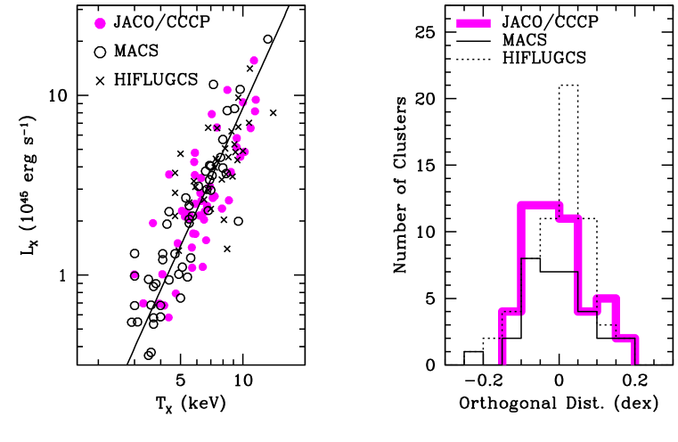
Figure 1.— Comparison of the luminosity-temperature relationship for JACO/CCCP sample (solid dots), HIFLUGS (open dots) and MACS (stars)

.

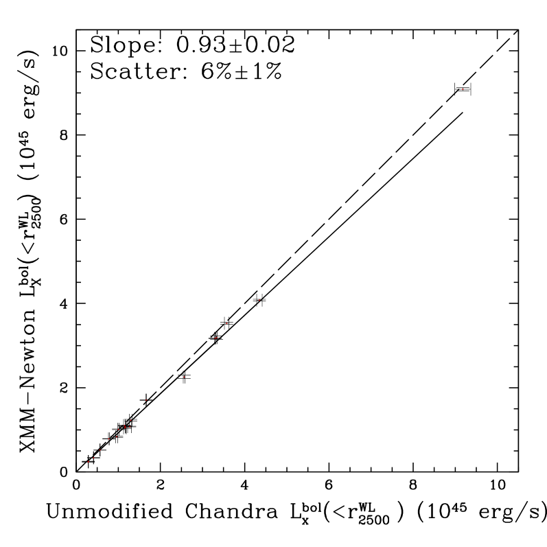
Figure 2.— Comparison of XMM-Newton and Chandra X-ray masses (top), temperatures (middle), and bolometric X-ray luminosities (bottom) within lensing $r_{2500}^{WL}$. The left-hand column shows the unmodified Chandra values, while the right-hand column shows the result of scaling the Chandra effective area by a power law in energy of slope $\zeta=0.07$, Chandra and XMM-Newton observables come into better agreement. The dashed line shows equality in all cases.

2.2. Choice of density contrast

For most of what follows, we study masses, temperatures, substructure measures, and other thermodynamic quantities integrated within a specific spherical radius. The choice of this radius is not obvious; using fixed physical radii has the advantage of straighforwardness, but the disadvantage that we would be probing characteristically different regions of clusters as a function of masses. Using fixed overdensity radii $r_{\Delta}$ (defined such that $r_{\Delta}$ contains a mean matter density of $\Delta$ times the critical density of the universe at the redshift of the cluster) is a better choice, but even here, the value of $\Delta$ to use is not quite obvious. At the redshift of our sample, X-ray data quality tends to be best around $r_{2500}$, but most of the literature lists properties at $r_{500}$. Even after a choice of $\Delta$, one must still decide whether to use the lensing or X-ray value, since they are not guaranteed to agree.

We choose to standardize the bulk of our discussion on the weak-lensing overdensity radius $r_{500}^{WL}$, because lensing masses are likely to be more unbiased for non-relaxed clusters (Meneghetti10). For the most part, our results do not significantly change if we switch to X-ray $r_{500}$; one exception is the mass-temperature relation below, which tightens significantly with the switch. In §5.3, we also consider scaling relations with observables measured within fixed physical radii, because these are more likely to be useful for calibrating large data sets.

2.3. Weak Lensing Overview

The clusters in our sample were drawn from Hoekstra12, which contains a weak lensing analysis of CFH12k and Megacam data from the Canada-France-Hawaii Telescope. We refer interested readers to Hoekstra12 for details of the data reduction and weak lensing analysis procedure.

We base our lensing masses on the aperture mass estimates (for details see the discussion in §3.5 in Hoekstra07). This approach has the advantage that it is practically model independent. Additionally, as the mass estimate relies only on shear measurements at large radii, contamination by cluster members is minimal. Hoekstra07 and Hoekstra12 removed galaxies that lie on the cluster red-sequence and boosted the signal based on excess number counts of galaxies. As an extreme scenario we omitted those corrections and found that the lensing masses change by only a few percent; for details see (Hoekstra12). Hence our masses are robust against contamination by cluster members at the percent level.

The weak lensing signal, however, only provides a direct estimate of the projected mass. To calculate 3D masses from the model-independent 2D aperture masses we project and renormalize a density profile of the form $\rho_{\mathrm{tot}}(r)\propto r^{-1}(r_{200}+cr)^{-2}$ (NFW). The relationship between the concentration $c$ and the virial mass is fixed at $c\propto M_{\mathrm{200}}^{-0.14}/(1+z)$ from numerical simulations (Duffy08). Hence, the deprojection itself, though well motivated based on numerical simulations, is model dependent. However, the model dependence is weak—20% variations in the normalization of the mass-concentration relationship yield $\approx 5\%$ variations in the measured masses (Hoekstra12, §4.3). We also note that the lensing analysis differs from the X-ray analysis in that in the X-ray analysis, no mass-concentration relationship is assumed (i.e., the concentrations and masses are allowed to vary independently). We plan to address the effects of relaxing the lensing mass-concentration relation in a future paper.

2.4. X-ray Data Reduction

We refer the reader to Mahdavi07 for details of the X-ray data reduction procedure, which we briefly summarize and update here. We use both Chandra CALDB 4.2.2 (April 2010) and CALDB 4.4.7 (December 2011). We also check our results against the latest CALDB (4.5.1) at the time of writing. For XMM-Newton we use calibration files up-to-date to January 2012; we also checked calibration files dating as far back as April 2010. We detected no statistically significant changes in the calibration files over this period for either Chandra or XMM-Newton, except as detailed in §2.6 below.

We follow a standard data reduction procedure. We use the software packages CIAO (Chandra) and SAS (XMM-Newton) to process raw event files using the recommended settings for each observation mode and detector temperature. Where possible, we make event grade selections that maximize the data quality for extended sources (including the VFAINT mode optimizations for Chandra). We use the wavelet detection algorithm WAVDETECT on exposure-corrected images to identify contaminating sources; we masked out point and extended sources using the detected wavelet radius. Each masking was checked by eye for missing extended sources or underestimated masking radii.

The bulk of the X-ray background consists of a particle component which bypasses the mirror assembly, plus an astrophysical component that is folded through the mirror response. To remove the particle background we match the 8-12 keV photon count rate from the outer regions of each detector to the recommended blank sky observations for each detector, and then subtract the renormalized blank-sky spectra. What remains is the source plus an over- or under-subtracted astrophysical background, plus in some cases residual particle background. All these residual backgrounds are modeled jointly with the spatially resolved ICM model spectra, and their parameters marginalized over for the final results.

To extract spatially resolved spectra, we find the surface brightness peak in the Chandra image (if available) or XMM-Newton image (if Chandra is not available). We then draw circular annuli that contain a minimum of 1500 background-subtracted photon counts; where both Chandra and XMM-Newton data are available, the annuli are taken to be exactly the same for both sets of observations, with the minimum count requirement being imposed on the Chandra data (for photons within 8$\arcmin$) or XMM-Newton data (for photons outside 8$\arcmin$). We then compute appropriately weighted ancilliary response files (ARF) and redistribution matrix files (RMF) for each spectrum, and subtract appropriately scaled particle background spectra. We emphasize that all spectra for each cluster undergo a simultaneous joint fit using a forward-convolved spectral model of the entire cluster, so that the choice of 1500 background-subtracted counts is not a sensitivity-limiting factor. That is to say, in no case is a single measurement derived from a single spectrum of 1500 counts, but rather such spectra are fit together in large batches on a cluster-by-cluster basis.

The detailed properties of the sample, including global X-ray temperatures and bolometric X-ray luminosities, masses, and substructure measures are listed in tables 2.4 and 2.6.

Table 1Basic Properties of the Sample

Cluster	RA	DEC	$z$	Chandra	Exposure	XMM-Newton	Exposure	$L_{\mathrm{X,all,bol,500}}$	$T_{\mathrm{all,500}}$
Name	J2000	J2000		ObsID	s	ObsID	s	keV	$10^{45}$ erg s-1
3C295	14:11:20.52	+52:12:09.9	0.464	2254	87914	$\cdots$	$\cdots$	$1.16\pm 0.02$	$5.7\pm 0.3$
Abell0068	00:37:06.65	+09:09:24.0	0.255	3250	9986	0084230201	14068	$1.43\pm 0.02$	$6.3\pm 0.4$
Abell0115N	00:55:50.37	+26:24:36.6	0.197	3233	49719	0203220101	21393	$1.11\pm 0.01$	$5.3\pm 0.2$
Abell0115S	00:56:00.17	+26:20:29.5	0.197	3233	49719	0203220101	21309	$1.17\pm 0.01$	$5.4\pm 0.3$
Abell0209	01:31:53.42	-13:36:46.3	0.206	3579	9986	0084230301	11219	$1.77\pm 0.02$	$7.0\pm 0.4$
Abell0222	01:37:34.25	-12:59:30.8	0.207	4967	45078	0502020201	23178	$0.50\pm 0.01$	$4.1\pm 0.3$
Abell0223S	01:37:56.06	-12:49:12.8	0.207	4967	45078	0502020201	23206	$0.62\pm 0.01$	$6.3\pm 0.4$
Abell0267	01:52:42.38	+01:00:48.0	0.231	3580	19624	0084230401	10421	$1.15\pm 0.03$	$6.5\pm 0.5$
Abell0370	02:39:53.18	-01:34:34.9	0.375	515	68532	$\cdots$	$\cdots$	$1.55\pm 0.06$	$7.2\pm 0.6$
Abell0383	02:48:03.33	-03:31:45.1	0.187	2320	19285	0084230501	20237	$0.96\pm 0.01$	$3.7\pm 0.1$
Abell0520	04:54:10.10	+02:55:18.3	0.199	4215	66274	0201510101	21915	$1.58\pm 0.02$	$7.3\pm 0.2$
Abell0521	04:54:06.30	-10:13:16.9	0.253	901	38626	$\cdots$	$\cdots$	$1.37\pm 0.02$	$5.9\pm 0.3$
Abell0586	07:32:20.16	+31:37:56.6	0.171	530	10043	$\cdots$	$\cdots$	$1.19\pm 0.02$	$5.1\pm 0.4$
Abell0611	08:00:56.96	+36:03:22.0	0.288	3194	36114	$\cdots$	$\cdots$	$1.61\pm 0.05$	$8.7\pm 0.6$
Abell0697	08:42:57.29	+36:21:56.2	0.282	4217	19516	$\cdots$	$\cdots$	$3.15\pm 0.07$	$10.3\pm 0.7$
Abell0851	09:43:00.39	+46:59:20.4	0.407	$\cdots$	$\cdots$	0106460101	15731	$0.93\pm 0.03$	$6.1\pm 0.4$
Abell0959	10:17:35.61	+59:33:53.4	0.286	$\cdots$	$\cdots$	0406630201	4134	$0.58\pm 0.03$	$6.0\pm 1.7$
Abell0963	10:17:03.63	+39:02:48.3	0.206	903	36289	0084230701	17234	$1.57\pm 0.01$	$6.2\pm 0.2$
Abell1689	13:11:29.52	-01:20:29.8	0.183	6930	76144	0093030101	24457	$4.48\pm 0.02$	$10.9\pm 0.2$
Abell1758E	13:32:46.43	+50:32:25.9	0.279	2213	55220	$\cdots$	$\cdots$	$2.33\pm 0.06$	$8.9\pm 0.6$
Abell1758W	13:32:38.70	+50:33:23.0	0.279	2213	55220	$\cdots$	$\cdots$	$1.46\pm 0.06$	$8.7\pm 1.0$
Abell1763	13:35:18.16	+40:59:57.7	0.223	3591	19595	0084230901	8852	$1.91\pm 0.03$	$6.3\pm 0.2$
Abell1835	14:01:01.90	+02:52:42.7	0.253	6880	117918	0098010101	16021	$4.51\pm 0.02$	$7.1\pm 0.1$
Abell1914	14:26:02.80	+37:49:27.3	0.171	3593	18865	0112230201	17025	$2.97\pm 0.02$	$9.7\pm 0.2$
Abell1942	14:38:21.90	+03:40:12.9	0.224	3290	55716	$\cdots$	$\cdots$	$0.33\pm 0.01$	$4.0\pm 0.3$
Abell2104	15:40:08.09	-03:18:16.5	0.153	895	49199	$\cdots$	$\cdots$	$2.32\pm 0.04$	$5.8\pm 0.3$
Abell2111	15:39:41.74	+34:25:01.9	0.229	544	10299	$\cdots$	$\cdots$	$0.91\pm 0.03$	$5.6\pm 0.7$
Abell2163	16:15:46.05	-06:09:02.6	0.203	1653	71148	$\cdots$	$\cdots$	$6.45\pm 0.10$	$11.5\pm 0.7$
Abell2204	16:32:46.92	+05:34:32.4	0.152	7940	77141	0306490201	13093	$3.99\pm 0.01$	$7.6\pm 0.1$
Abell2218	16:35:50.89	+66:12:36.9	0.176	1666	30693	0112980101	13111	$1.28\pm 0.02$	$6.6\pm 0.2$
Abell2219	16:40:20.20	+46:42:35.3	0.226	896	42295	$\cdots$	$\cdots$	$6.45\pm 0.08$	$8.3\pm 0.3$
Abell2259	17:20:07.75	+27:40:14.7	0.164	3245	9986	$\cdots$	$\cdots$	$0.77\pm 0.02$	$5.0\pm 0.3$
Abell2261	17:22:27.12	+32:07:58.9	0.224	5007	24316	$\cdots$	$\cdots$	$2.59\pm 0.03$	$5.6\pm 0.3$
Abell2390	21:53:36.82	+17:41:44.7	0.228	4193	93782	0111270101	8100	$5.99\pm 0.03$	$10.1\pm 0.3$
Abell2537	23:08:22.23	-02:11:30.3	0.295	4962	36193	0205330501	6267	$1.37\pm 0.03$	$6.9\pm 0.7$
CL0024.0+1652	00:26:35.94	+17:09:46.2	0.390	929	39417	$\cdots$	$\cdots$	$0.34\pm 0.02$	$4.5\pm 0.8$
MACSJ0717.5+3745	07:17:31.39	+37:45:24.8	0.548	4200	58912	$\cdots$	$\cdots$	$5.55\pm 0.12$	$11.6\pm 0.7$
MACSJ0913.7+4056	09:13:45.49	+40:56:28.7	0.442	10445	76159	$\cdots$	$\cdots$	$1.99\pm 0.04$	$6.0\pm 0.2$
MS0015.9+1609	00:18:33.74	+16:26:09.0	0.541	520	67410	0111000101	22477	$3.73\pm 0.10$	$9.5\pm 0.6$
MS0440.5+0204	04:43:09.99	+02:10:19.3	0.190	4196	22262	$\cdots$	$\cdots$	$0.33\pm 0.01$	$3.3\pm 0.3$
MS0451.6-0305	04:54:11.24	-03:00:57.3	0.550	902	43420	$\cdots$	$\cdots$	$3.25\pm 0.12$	$9.2\pm 0.8$
MS0906.5+1110	09:09:12.73	+10:58:28.4	0.174	924	29752	$\cdots$	$\cdots$	$1.10\pm 0.02$	$5.6\pm 0.3$
MS1008.1-1224	10:10:32.52	-12:39:53.1	0.301	926	25222	$\cdots$	$\cdots$	$0.77\pm 0.02$	$5.9\pm 0.5$
MS1231.3+1542	12:33:55.01	+15:26:02.3	0.233	$\cdots$	$\cdots$	0404120101	26520	$0.29\pm 0.01$	$4.5\pm 0.2$
MS1358.1+6245	13:59:50.56	+62:31:05.3	0.328	516	50989	$\cdots$	$\cdots$	$1.19\pm 0.03$	$6.2\pm 0.5$
MS1455.0+2232	14:57:15.05	+22:20:33.2	0.258	4192	91626	0108670201	22571	$1.84\pm 0.01$	$4.4\pm 0.1$
MS1512.4+3647	15:14:22.47	+36:36:20.9	0.372	800	36400	$\cdots$	$\cdots$	$0.48\pm 0.02$	$3.1\pm 0.2$
MS1621.5+2640	16:23:35.05	+26:34:22.1	0.426	546	30062	$\cdots$	$\cdots$	$0.89\pm 0.04$	$6.9\pm 0.8$
RXJ1347.5-1145	13:47:30.59	-11:45:09.8	0.451	3592	57458	0112960101	21712	$10.96\pm 0.18$	$12.1\pm 0.4$
RXJ1524.6+0957	15:24:38.85	+09:57:41.8	0.520	1664	49849	$\cdots$	$\cdots$	$0.41\pm 0.03$	$4.7\pm 1.2$

2.5. X-ray Mass Modeling

Here we summarize and update the modeling procedure of Mahdavi07, in which the cluster is spherically symmetric and that the gas is in thermal pressure supported hydrostatic equilibrium within the cluster potential. The essence of the technique is to directly compare the observed spatially resolved spectra with model predictions. For a spectrum observed in an annulus with inner and outer radii $R_{1}$ and $R_{2}$, the model is

$$L_{\nu}=\int_{R_{1}}^{R_{2}}2\pi RdR\int_{R}^{r_{\mathrm{max}}}n_{e}n_{H}\Lambda_{\nu}[T(r),Z(r)]\frac{2rdr}{\sqrt{r^{2}-R^{2}}}$$ (1)

where $r$ denotes unprojected radius, $R$ denotes projected radius, $r_{\mathrm{max}}$ is the termination radius of the X-ray gas (taken to be $r_{100}$ in this paper), $\Lambda_{\nu}$ is the frequency-dependent cooling function which is a function of temperature $T$ and metallicity $Z$, and $n_{e}$ and $n_{H}$ are the electron and hydrogen number density, respectively.

One feature of the above method is that the unprojected temperature profile is calculated self-consistently assuming hydrostatic equilibrium of assumed gas and dark matter density profiles. As a result, we never have to specify or fit a temperature profile; temperature is merely an intermediate “dummy” quantity connecting the gas and dark matter mass distributions to the X-ray spectra. This avoids subjective weighting involved in the fitting of 2D projected temperature profiles (Mazzotta04; Rasia05; Vikhlinin06b), which are more difficult to correct for the effects of PSF distortion.

2.6. Parameters of the Hydrostatic Model

The hydrostatic model assumes a flexible spherical electron density distribution

$$n(r) = n_{e_{0}}\left(\frac{r}{r_{x_{0}}}\right)^{-\alpha}B(r,r_{x_{0}},\beta_{0})+$$

$$n_{e_{1}}B(r,r_{x_{1}},\beta_{1})+n_{e_{2}}B(r,r_{x_{2}},\beta_{2})$$

where the familiar “beta” model is

$$B(r,r_{x_{i}},\beta_{i})=\left(1+\frac{r}{r_{x_{i}}}\right)^{-\frac{3\beta_{i}}{2}}$$

In other words, the gas mass profile consists of a fully general triple “beta” model profile, where the first beta model is further allowed to be multiplied by a single power law. The metallicity distribution is modeled as (e.g. Pizzolato03)

$$\frac{Z}{Z_{\odot}}=Z_{0}\left(1+\frac{r^{2}}{r_{z}^{2}}\right)^{-3\beta_{z}}$$ (3)

with $r_{Z}$, $\beta_{z}$, and $Z_{0}$ free parameters. Finally, the total mass distribution (baryons and dark matter) are modeled as a NFW profile:

$$\rho_{\mathrm{tot}}=\frac{M_{0}}{r(cr+r_{\Delta})^{2}}$$ (4)

where $M_{0}$ is the normalization, $c$ is the halo concentration, and $r_{\Delta}$ is the overdensity radius (see above). These are also free parameters, except that rather than fitting $M_{0}$, we fit $M_{\Delta}$—the mass within $r_{\Delta}$—as the normalization constant (because there is a one-to-one relationship between $M_{0}$ and $M_{\Delta}$).

In general, some of the above parameters are better determined than the others. For example, the inner slope of the gas density distribution, $\alpha$, is always well measured (with a typical uncertainty of $\pm 0.1$, and follows the well-known trend (e.g Sanderson10) that low central entropy clusters have steeper inner profiles, $\alpha\approx 0.5$, whereas high entropy clusters have flatter profiles, $\alpha\approx 0$). The central metallicities are similarly well-determined. On the other hand, quantities such as the slopes and core radii of multiple $\beta$-model profiles—such as $\beta_{2}$ and $\beta_{3}$ or $r_{Z}$ and $\beta_{Z}$—frequently reveal significant degeneracies with each other. In all cases, such degeneracies are properly marginalized over using the Hrothgar Markov chain monte carlo procedure described in Mahdavi07, and the one-dimensional error bars in Table 2.6 always properly reflect any and all degeneracies among the many parameters in this many-dimensional model.

Table 2Mass and Substructure Properties at $r_{500}$

Cluster	$r_{500}^{\mathrm{WL}}$	$M_{\mathrm{WL}}$	$M_{\mathrm{Gas}}$	$M_{\mathrm{hydro}}$	$K_{0}$		$D_{\mathrm{BCG}}$	$w_{X}$	$P3/P0$
	Mpc	$10^{14}M_{\odot}$	$10^{14}M_{\odot}$	$10^{14}M_{\odot}$	keV cm2		kpc	$10^{3}\times r_{500}^{\mathrm{WL}}$	$\times 10^{-7}$
3C295	$1.06\pm 0.06$	$5.7\pm 1.2$	$0.62\pm 0.03$	$3.9\pm 1.0$	$12.8$$\ \pm\$	$2.4$	$12$	$5.7\pm 1.4$	$0.25\pm 0.20$
Abell0068	$1.16\pm 0.09$	$5.9\pm 1.6$	$0.77\pm 0.01$	$5.1\pm 1.0$	$214.2$$\ \pm\$	$29.5$	$15$	$14.0\pm 2.1$	$0.74\pm 0.60$
Abell0115N	$1.03\pm 0.12$	$3.9\pm 1.5$	$0.60\pm 0.01$	$4.1\pm 0.2$	$30.0$$\ \pm\$	$2.4$	$10$	$59.6\pm 0.8$	$3.31\pm 0.82$
Abell0115S	$1.14\pm 0.07$	$5.3\pm 1.2$	$0.80\pm 0.01$	$4.2\pm 0.3$	$192.8$$\ \pm\$	$48.5$	$143$	$\cdots$	$\cdots$
Abell0209	$1.24\pm 0.07$	$6.8\pm 1.4$	$1.02\pm 0.02$	$5.6\pm 1.1$	$152.7$$\ \pm\$	$20.9$	$16$	$7.1\pm 1.1$	$1.47\pm 1.10$
Abell0222	$1.16\pm 0.07$	$5.7\pm 1.3$	$0.61\pm 0.01$	$2.4\pm 0.6$	$220.2$$\ \pm\$	$32.2$	$10$	$38.4\pm 3.2$	$1.21\pm 0.96$
Abell0223S	$1.24\pm 0.10$	$6.9\pm 2.0$	$0.68\pm 0.04$	$3.3\pm 1.6$	$133.5$$\ \pm\$	$20.1$	$8$	$36.9\pm 2.4$	$2.26\pm 1.62$
Abell0267	$1.13\pm 0.09$	$5.3\pm 1.5$	$0.63\pm 0.01$	$5.7\pm 0.6$	$160.8$$\ \pm\$	$20.6$	$77$	$22.0\pm 1.7$	$0.27\pm 0.22$
Abell0370	$1.43\pm 0.06$	$12.8\pm 2.0$	$1.00\pm 0.05$	$8.6\pm 6.0$	$500.1$$\ \pm\$	$159.8$	$23$	$15.8\pm 1.3$	$0.62\pm 0.49$
Abell0383	$1.04\pm 0.13$	$4.0\pm 1.8$	$0.39\pm 0.01$	$4.6\pm 0.6$	$21.3$$\ \pm\$	$1.0$	$<3$	$3.1\pm 0.6$	$0.36\pm 0.26$
Abell0520	$1.16\pm 0.07$	$5.6\pm 1.3$	$0.85\pm 0.01$	$7.3\pm 0.3$	$590.1$$\ \pm\$	$39.4$	$341$	$100.7\pm 0.7$	$4.66\pm 0.97$
Abell0521	$1.19\pm 0.08$	$6.3\pm 1.6$	$1.06\pm 0.02$	$5.0\pm 1.3$	$75.6$$\ \pm\$	$18.1$	$33$	$58.5\pm 1.7$	$8.59\pm 3.41$
Abell0586	$1.18\pm 0.09$	$5.6\pm 1.6$	$0.65\pm 0.08$	$3.9\pm 0.6$	$140.1$$\ \pm\$	$23.5$	$11$	$7.3\pm 1.6$	$0.59\pm 0.49$
Abell0611	$1.13\pm 0.06$	$5.7\pm 1.3$	$0.66\pm 0.05$	$6.0\pm 0.9$	$57.0$$\ \pm\$	$9.0$	$4$	$8.0\pm 0.8$	$0.68\pm 0.42$
Abell0697	$1.35\pm 0.05$	$9.7\pm 1.3$	$1.56\pm 0.03$	$10.9\pm 1.5$	$240.0$$\ \pm\$	$45.4$	$20$	$9.1\pm 1.1$	$0.20\pm 0.16$
Abell0851	$1.32\pm 0.09$	$10.5\pm 2.5$	$0.97\pm 0.02$	$7.4\pm 2.3$	$479.7$$\ \pm\$	$79.7$	$278$	$30.5\pm 3.4$	$13.15\pm 7.51$
Abell0959	$1.26\pm 0.07$	$7.8\pm 1.7$	$0.75\pm 0.03$	$5.6\pm 0.5$	$203.8$$\ \pm\$	$23.7$	$36$	$42.6\pm 4.5$	$7.70\pm 6.55$
Abell0963	$1.00\pm 0.10$	$3.7\pm 1.3$	$0.57\pm 0.01$	$4.7\pm 0.5$	$63.1$$\ \pm\$	$5.9$	$6$	$5.5\pm 0.5$	$0.12\pm 0.10$
Abell1689	$1.57\pm 0.09$	$13.7\pm 2.7$	$1.27\pm 0.01$	$9.7\pm 0.6$	$72.5$$\ \pm\$	$5.5$	$5$	$4.1\pm 0.3$	$0.08\pm 0.04$
Abell1758E	$1.37\pm 0.08$	$10.1\pm 2.3$	$1.23\pm 0.04$	$9.4\pm 0.6$	$227.4$$\ \pm\$	$28.5$	$25$	$117.9\pm 1.2$	$8.42\pm 1.62$
Abell1758W	$1.37\pm 0.06$	$10.0\pm 1.4$	$0.93\pm 0.07$	$11.5\pm 1.6$	$194.5$$\ \pm\$	$19.9$	$25$	$117.9\pm 1.2$	$8.42\pm 1.62$
Abell1763	$1.40\pm 0.10$	$10.1\pm 2.5$	$1.34\pm 0.01$	$3.9\pm 0.7$	$419.5$$\ \pm\$	$54.0$	$7$	$22.9\pm 1.2$	$0.97\pm 0.64$
Abell1835	$1.30\pm 0.05$	$8.4\pm 1.3$	$1.21\pm 0.01$	$9.9\pm 0.7$	$19.7$$\ \pm\$	$0.4$	$6$	$3.9\pm 0.2$	$<0.1$
Abell1914	$1.18\pm 0.05$	$5.6\pm 1.0$	$0.99\pm 0.00$	$9.2\pm 0.9$	$128.7$$\ \pm\$	$9.5$	$86$	$27.8\pm 0.5$	$2.39\pm 0.40$
Abell1942	$1.05\pm 0.06$	$4.3\pm 1.0$	$0.44\pm 0.01$	$2.7\pm 0.6$	$230.6$$\ \pm\$	$72.2$	$4$	$9.3\pm 1.4$	$1.57\pm 1.21$
Abell2104	$1.22\pm 0.08$	$6.1\pm 1.6$	$0.68\pm 0.14$	$5.8\pm 0.8$	$201.7$$\ \pm\$	$44.2$	$8$	$\cdots$	$\cdots$
Abell2111	$1.07\pm 0.10$	$4.5\pm 1.5$	$0.74\pm 0.07$	$7.3\pm 2.5$	$203.8$$\ \pm\$	$55.6$	$129$	$33.0\pm 2.8$	$3.22\pm 2.43$
Abell2163	$1.38\pm 0.11$	$9.5\pm 2.5$	$2.33\pm 0.03$	$12.0\pm 1.2$	$336.0$$\ \pm\$	$18.0$	$160$	$35.3\pm 0.4$	$3.76\pm 0.37$
Abell2204	$1.34\pm 0.07$	$8.1\pm 1.6$	$1.16\pm 0.01$	$8.7\pm 0.6$	$17.3$$\ \pm\$	$0.3$	$<3$	$4.8\pm 0.3$	$<0.1$
Abell2218	$1.14\pm 0.08$	$5.1\pm 1.4$	$0.72\pm 0.01$	$4.3\pm 0.6$	$317.9$$\ \pm\$	$44.9$	$60$	$18.9\pm 1.0$	$1.28\pm 0.53$
Abell2219	$1.35\pm 0.07$	$9.1\pm 1.9$	$1.65\pm 0.03$	$7.1\pm 0.9$	$243.2$$\ \pm\$	$33.3$	$8$	$\cdots$	$\cdots$
Abell2259	$1.05\pm 0.09$	$4.0\pm 1.2$	$0.50\pm 0.04$	$4.1\pm 0.9$	$134.7$$\ \pm\$	$30.1$	$78$	$24.1\pm 1.7$	$1.18\pm 0.95$
Abell2261	$1.52\pm 0.05$	$12.9\pm 1.6$	$1.46\pm 0.13$	$6.6\pm 1.0$	$60.0$$\ \pm\$	$9.0$	$<2$	$14.3\pm 1.0$	$0.39\pm 0.21$
Abell2390	$1.33\pm 0.06$	$8.6\pm 1.5$	$1.48\pm 0.01$	$11.0\pm 0.9$	$31.6$$\ \pm\$	$1.1$	$4$	$11.1\pm 0.9$	$1.24\pm 0.17$
Abell2537	$1.22\pm 0.05$	$7.2\pm 1.1$	$0.86\pm 0.06$	$5.9\pm 0.9$	$91.8$$\ \pm\$	$21.7$	$17$	$8.4\pm 1.3$	$0.99\pm 0.74$
CL0024.0+1652	$1.30\pm 0.10$	$9.8\pm 2.7$	$0.45\pm 0.08$	$3.1\pm 4.7$	$61.2$$\ \pm\$	$15.9$	$24$	$73.5\pm 11.5$	$6.46\pm 5.23$
MACSJ0717.5+3745	$1.46\pm 0.07$	$16.6\pm 3.4$	$2.35\pm 0.03$	$12.3\pm 1.9$	$396.3$$\ \pm\$	$80.0$	$224$	$23.9\pm 0.9$	$23.09\pm 3.24$
MACSJ0913.7+4056	$0.95\pm 0.07$	$4.0\pm 1.3$	$0.53\pm 0.02$	$4.8\pm 0.7$	$17.0$$\ \pm\$	$1.1$	$4$	$4.3\pm 1.0$	$0.40\pm 0.19$
MS0015.9+1609	$1.60\pm 0.06$	$21.9\pm 3.2$	$2.01\pm 0.06$	$13.4\pm 1.9$	$171.0$$\ \pm\$	$20.0$	$41$	$8.6\pm 1.1$	$0.58\pm 0.38$
MS0440.5+0204	$0.85\pm 0.06$	$2.2\pm 0.7$	$0.24\pm 0.05$	$2.8\pm 0.5$	$30.1$$\ \pm\$	$5.7$	$<3$	$19.6\pm 4.2$	$1.38\pm 1.16$
MS0451.6-0305	$0.95\pm 0.10$	$4.5\pm 1.7$	$1.03\pm 0.02$	$7.8\pm 1.0$	$235.3$$\ \pm\$	$43.3$	$28$	$11.9\pm 1.1$	$1.44\pm 0.82$
MS0906.5+1110	$1.36\pm 0.09$	$8.7\pm 1.9$	$0.87\pm 0.03$	$3.5\pm 0.5$	$148.9$$\ \pm\$	$29.0$	$3$	$17.1\pm 1.2$	$0.20\pm 0.14$
MS1008.1-1224	$1.06\pm 0.05$	$4.8\pm 0.9$	$0.58\pm 0.04$	$7.3\pm 3.1$	$97.9$$\ \pm\$	$24.7$	$10$	$55.8\pm 2.2$	$4.17\pm 2.33$
MS1231.3+1542	$0.54\pm 0.11$	$0.6\pm 0.4$	$0.14\pm 0.00$	$1.4\pm 0.1$	$131.5$$\ \pm\$	$16.5$	$72$	$6.9\pm 1.4$	$5.08\pm 3.82$
MS1358.1+6245	$1.12\pm 0.09$	$5.9\pm 1.6$	$0.67\pm 0.07$	$7.6\pm 0.9$	$39.3$$\ \pm\$	$3.9$	$4$	$8.6\pm 1.2$	$0.34\pm 0.29$
MS1455.0+2232	$1.04\pm 0.05$	$4.2\pm 0.8$	$0.56\pm 0.01$	$3.1\pm 0.2$	$23.6$$\ \pm\$	$0.8$	$3$	$4.9\pm 0.2$	$0.13\pm 0.06$
MS1512.4+3647	$0.85\pm 0.18$	$2.6\pm 1.8$	$0.34\pm 0.03$	$2.1\pm 0.7$	$26.4$$\ \pm\$	$8.1$	$6$	$6.7\pm 1.3$	$1.30\pm 1.09$
MS1621.5+2640	$1.19\pm 0.07$	$7.7\pm 1.8$	$0.83\pm 0.03$	$5.4\pm 0.8$	$182.1$$\ \pm\$	$37.7$	$41$	$19.0\pm 4.3$	$7.47\pm 5.43$
RXJ1347.5-1145	$1.25\pm 0.12$	$9.3\pm 2.9$	$1.63\pm 0.01$	$13.1\pm 1.8$	$29.7$$\ \pm\$	$2.1$	$<4$	$12.6\pm 1.4$	$1.30\pm 0.41$
RXJ1524.6+0957	$0.87\pm 0.12$	$3.4\pm 1.8$	$0.41\pm 0.04$	$2.7\pm 0.4$	$123.9$$\ \pm\$	$42.3$	$22$	$63.2\pm 5.6$	$22.92\pm 15.12$

2.7. Joint Calibration of Chandra and XMM-Newton Masses

Where available, we use both Chandra and XMM-Newton data for a cluster. This has several advantages: in the inner regions, Chandra is able to resolve the cluster cores well; while XMM-Newton’s wider field of view yields better coverage of the outer regions of the cluster. The simultaneous coverage of intermediate regions helps constrain residual backgrounds following blank sky subtraction.

When combining Chandra and XMM-Newton data, cross-calibration is a significant issue. In general, there are slight differences among the responses of the Chandra ACIS and the XMM-Newton pn, MOS1, and MOS2 detectors. Even after over a decade in flight, the source of these differences has not been conclusively identified. Typically, comparisons show that Chandra temperatures are $5-15\%$ higher (Snowden08; Reese10). The most recent calibration tests (Tsujimoto11) use the G21.5-0.9 pulsar (which is fainter than the usual source, the Crab nebula, and hence not subject to detector pileup). Tsujimoto11 find that the XMM-Newton pn has a 15% lower flux in the 2.0-8.0 keV energy band compared to the Chandra ACIS-S. This confirms an earlier finding by Nevalainen10 who found similar results. Lower hard band flux naturally leads to lower X-ray temperatures when 0.5-2.0 keV photons are also included. This primarily affects masses for which spectral line emission is not dominant (i.e., in hot, k T $>4$ keV clusters). It is at this point unknown where the source of the disagreement lies and which instrument is better calibrated.

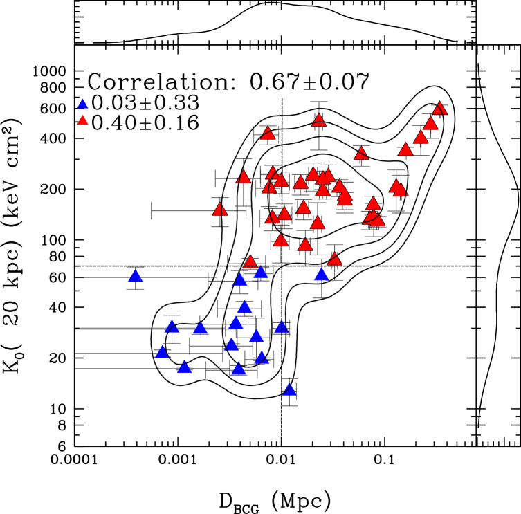
Figure 3.— Bimodality in the joint distribution of BCG offset and central entropy; contours show lines of constant probability density after the points have been smoothed with a 0.25 dex Gaussian. The top and right axes show the 1D probability density for central entropy and BCG offset. Blue triangles show cool-core clusters and red triangles show non-cool-core clusters. The horizontal thin line shows our chosen division between cool-core and non-cool-core systems, while the vertical line shows our chosen division between low BCG offset and high BCG offset systems.

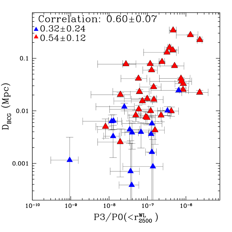
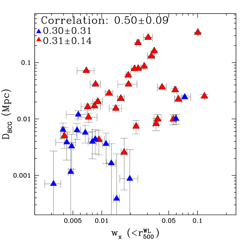
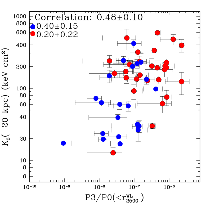
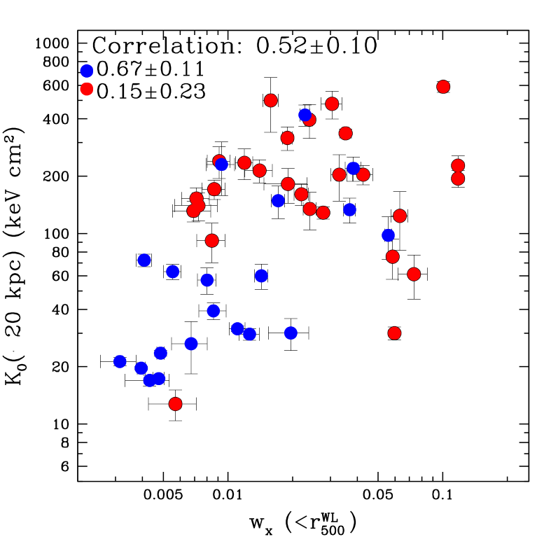
Figure 4.— Correlation of four different substructure measures (central entropy $K_{0}$, BCG offset $D_{\mathrm{BCG}}$, X-ray centroid variance $w_{X}$, and $P3/P0$ power ratio) against each other. Blue triangles show cool-core clusters and red triangles show non-cool-core clusters; blue circles show low-BCG-offset systems and red circles show high-BCG-offset systems.

Figure 2 shows the X-ray mass measured within lensing $r_{2500}^{WL}$ for the 19 clusters in our sample which contain both Chandra and XMM-Newton data. Shown are the results for CALDB 4.2.2 (April 2010). We also checked CALDB 4.4.7 (December 2011) and CALDB 4.5.1 (June 2012). The calibration for our sample changed little during this period, and in all three cases, we find that Chandra masses are higher than XMM-Newton masses by roughly 15%. All observations were recorded prior to 2010, and taken as a whole, the change in the Chandra masses of these systems is not statistically significant between CALDB 4.2.2 and 4.4.7. We adopt the 2010 CALDB for the remainder of this paper, stressing that any changes to our results would be well within the statistical errors presented were we to switch to a different calibration release.

To be able to combine Chandra and XMM-Newton data, one must first ensure that they are consistent. We find that the following simple cross-calibration prescription is able to bring the data into self-consistency:

$$A^{\mathrm{corrected}}_{\mathrm{CXO}}(E)=A_{\mathrm{CXO}}(E)\left(\frac{E}{\mathrm{keV}}\right)^{\zeta}$$ (5)

where $\zeta=0$ gives the unmodified CALDB area, and $\zeta>0$ has the effect of down-weighting the high energy effective area of Chandra. We find that setting $\zeta=0.07$ brings Chandra and XMM-Newton masses into agreement as shown in Figure 2. In either case, the intrinsic scatter between Chandra and XMM-Newton mass measurements at these fixed radii is certainly less than 10%, though inconsistent with zero at the 2$\sigma$ level.

Figure 2 also shows that the integrated X-ray temperatures and luminosities within lensing $r_{2500}$ are also improved by our suggested calibration. The discrepancy between unmodified Chandra X-ray temperatures and XMM temperatures is roughly the same as the discrepancy in hydrostatic masses. The bolometric X-ray luminosities are also in better agreement as a result of the effective area re-calibration, though in this case the original discrepancy is less severe than in the realm of the spectroscopic temperature.

We chose to modify the Chandra effective area, and not the XMM-Newton effective area, based on the fact that the XMM-Newton has exhibited the least variation over the years, whereas Chandra has enacted larger 10-15% changes in its effective area calibration historically. We note that had we modified the XMM-Newton effective area to match that of Chandra, then we would have found in what follows that clusters no longer exhibit self-similar behavior and that (a) those with obvious substructure would be the ones whose masses calculated assuming hydrostatic equilibrium would agree with their weak lensing masses, and (b) that clusters with cool cores would have hydrostatic masses greater than their weak lensing masses. This uncertainty in the telescopes’ effective areas must be viewed as a fundamental systematic limitation of X-ray astronomy at least as related to cluster science.

2.8. Online Data and Regression Tool

All data and analysis software used for this paper are available online at http://sfstar.sfsu.edu/cccp. Fits of scaling relations (i.e., the modeling of linear or power law relationships among measured quantities) are complicated by the fact that error in both coordinates makes ordinary $\chi^{2}$ analysis invalid. A detailed treatise of recent developments in the theory behind modeling 2D data with errors in both coordinates appears in Hogg10. These techniques allow the simultaneous estimation of slope, intercept, and intrinsic scatter in such relations. We implement the methods of Hogg10 at the data website for this article.

3. Measures of non-relaxed status

The gas in all clusters of galaxies exhibits some degree of deviation from an idealized smooth, triaxial distribution. Such deviation could come in terms of subclumping, asymmetry, or both. Its presence gives some clue as to the nature of its evolutionary history; for example, asymmetry could indicate either the beginning or the end of a merger event; subclumps could either be recently accreted small groups of galaxies, or surviving cold cores from recent mergers.

Despite this ambiguity, objective measures of substructure are helpful in arriving at quantitative estimates of departure from equilibrium. To begin, we employ two common and well-tested measures of substructure: power ratios and centroid shift variance. Power ratios are Fourier-space estimators of fluctuations in the overall cluster surface brightness distribution, while the centroid shift is a measure of the variance of the distance between the X-ray surface brightness peak (which is always well defined) and the centroid (which in a non-relaxed cluster often varies significantly as a function isophote used for its estimation). We refer the reader to Buote95; Poole06; Jeltema05; Jeltema08 and Boehringer10 for details on the calculation of these estimators.

As further tracers of the relaxed or nonrelaxed state of a system, we also consider the somewhat more straightforward measures, central entropy and the X-ray to optical center offset. Low central entropies indicate the presence of a cool core, which tend to be associated (non-exclusively) with relaxed clusters. We define the central entropy as:

$$K_{0}\equiv K(20\mathrm{kpc})$$ (6)

In other words, the central entropy is defined as the deprojected entropy profile evaluated at a radius of 20kpc from the cluster center.

Similarly, the distance between the brightest cluster galaxy (BCG) and the X-ray surface brightness peak can be a good predictor of relaxed state, with large shifts indicating ongoing or residual merger activity (Poole07). We measure this distance via simple astrometry on X-ray and optical images, and call it $D_{\mathrm{BCG}}$.

One would expect relaxed halos to be more representative of idealized halo growth models. Hence we expect scaling relations among the various thermodynamic and dark matter parameters to be tighter for clusters selected on the basis of the more well-behaved substructure indicators. We also expect the most powerful substructure measures to be correlated with each other.

3.1. Correlations among measures of substructure

We explore the possibility of whether our substructure measures show inherent correlation. The presence of such correlations, particularly when involving both X-ray and optical data, can serve as road maps towards our goal of quantifying departures from equilibrium as economically as possible. We use the Spearman’s rank correlation coefficient, with bootstrap resampling for determining $1\sigma$ uncertainties.

The relationship between central entropy and BCG offset is the most significant correlation in our sample. This also happens to be the most interesting correlation due to the relative ease of deriving central entropy and BCG offset from observables. Figure 3 shows that the two substructures measures appear to form a two-peaked joint distribution, with low central entropy, low BCG offsets in one corner, and high central entropy, high BCG offset clusters in another. The dividing line is best seen as a curve with equation

$$K_{0}=7\mathrm{\,keV\,cm}^{2}\left(\frac{D_{\mathrm{BCG}}}{\mathrm{Mpc}}\right)^{-1/2}$$ (7)

The high correlation coefficient between $K_{0}$ and $D_{\mathrm{BCG}}$ appears to be due to bimodality: when we calculate the correlation coefficient separately for either cloud, we find that the clouds individually do not contain significant internal correlation. Though the above formula offers the most clean separation between the two clouds, most of the separation can be captured by imposing cuts in entropy, or, somewhat less cleanly, in BCG offset.

For this reason, throughout the rest of the paper, we introduce a labeling system that represents cuts in these two most easily measured substructure estimators. We use blue triangles to indicate $K_{0}<70$ keV cm² (“cool core systems” or CC), and red triangles to indicate $K_{0}>70$ keV cm² (“non-cool-core systems” or NCC). This nomenclature is based on the fact that of 70 keV cm² corresponds to a cooling time of $\approx 1.5$ Gyr; most cool core clusters have central cooling times below this value.

Similarly, we use blue circles to indicate systems with $D_{\mathrm{BCG}}<0.01$ Mpc (“low BCG offset systems”) and red circles to indicate $D_{\mathrm{BCG}}>0.01$ Mpc (“high BCG offset systems”).

In Figure 4, we look for inherent correlations among the other various indicators of substructure. Strong correlations exist between the BCG offset $D_{\mathrm{BCG}}$, the central entropy $K_{0}$, the X-ray centroid shift $w_{X}$ at $r_{500}^{WL}$, and the P3/P0 ratio at $r_{2500}^{WL}$ (in measuring the latter two, we cut out the central 0.15 $r_{500}^{WL}$ to avoid dilution of the signal by the cool core). Interestingly, the P3/P0 ratio measured at $r_{500}^{WL}$ (instead of $r_{2500}^{WL}$) showed much larger scatter (presumably due to noise) and proved much less tightly correlated with the other substructure measures than the P3/P0 ratio at $r_{2500}^{WL}$.

In particular, it should be noted that $P3/P0$ exhibits almost as strong a correlation with BCG offset as does central entropy, though there is no evidence for bimodality. For non-cool-core clusters, the $P3/P0$ is significantly more correlated with BCG offset than is the central entropy. This is quite a surprising result, since $P3/P0$ traces cluster dynamics outside the cool core, whereas the central entropy is more sensitive to the inner parts.

The BCG correlation trends are consistent with the well-known tendency of cool cores to occur in smoother (i.e. more relaxed, hence lower $w_{X}$, low power ratio) clusters where a BCG sits close to the bottom of the potential well (Bildfell08). This demonstrates the tight quantitative link between these completely independent X-ray and optical indicators of substructure.

4. The $L_{X}$-$T_{X}$ Relation

Similarly to previous studies (e.g. Morandi07; Pratt10; Mittal11), we find that the luminosity-temperature ($L_{X}-T_{X}$) relationship exhibits a significant scatter of $\approx 50\%$ when the core of the cluster is included—a scatter which is diminished considerably, to 36%, when the core is excised. This effect is due to the overall non-self-similarity of cluster cool cores in comparison to the regions outside the cool core (e.g Vikhlinin06). When the core is not excised, the cool-core clusters lie significantly above the non-cool-core clusters, an effect first noted by Fabian94b and subsequently studied in detail by McCarthy04 and Maughan12.

In Figure 5 and Table 3, we show that when we include all cluster emission, the residuals of the $L_{X}-T_{X}$ relation show a strong and significant correlation with both the central entropy of the cluster and the centroid shift $w_{X}$ (we choose $w_{X}$ because of the four measures discussed in §3.1 it offers the strongest correlation). However, when we cut out the central 0.15 $r_{500}^{WL}$, the distinction disappears, and the cool-core and non-cool-core clusters become indistinguishable in terms of entropy as well as $w_{X}$. This is consistent with the findings of Maughan12 in the sense that once the cool core is taken out of consideration, residuals in the L-T relation no longer carry information regarding the dynamical state of the cluster.

This is an example of “irreversible scatter”—in other words, outside their cores, the clusters of galaxies in our sample have “forgotten” the cause of the intrinsic scatter in the $L_{X}$-$T_{X}$ relation. This has implications for scaling relation correction procedures such as described in (Jeltema08, e.g.), where relationship between the residuals and the substructure measures for simulated clusters are used to produce corrected observables which sit more tightly on the scaling relations. The lack of correlation in our case implies that such procedures will not reduce the scatter in the measured scaling relations (at least for the JACO/CCCP sample).

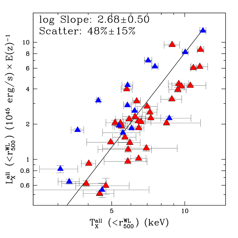
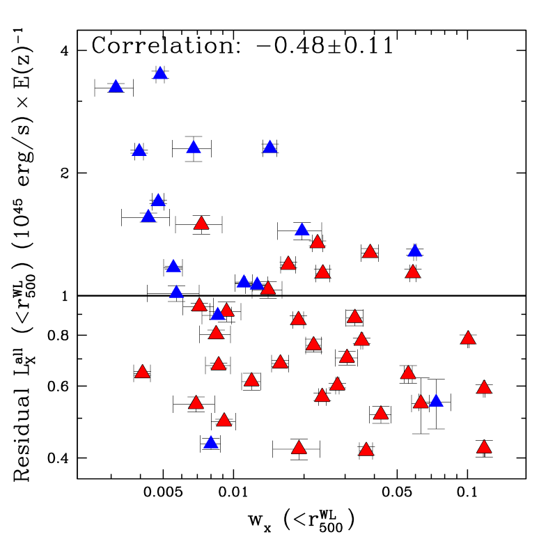
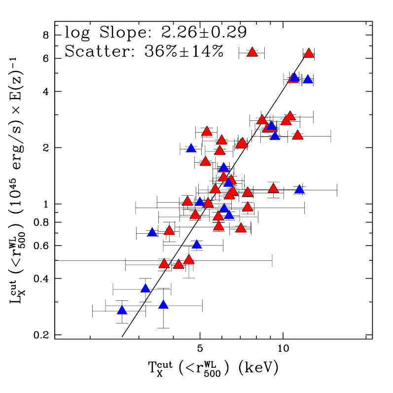
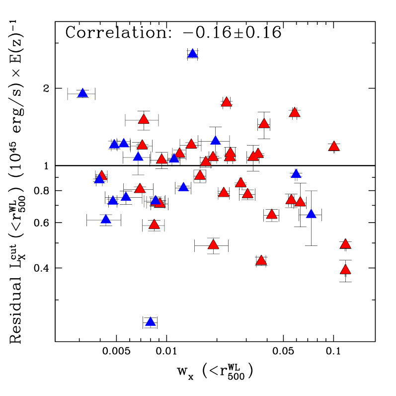
Figure 5.— (top panels) The luminosity-temperature relationship at lensing $r_{500}^{WL}$ and its residuals compared to centroid shift variance $w_{X}$. (bottom panels) same as top, except that the inner 0.15 $r_{500}^{WL}$ has been removed. The residuals are uncorrelated with all four substructure measures. Blue triangles show cool-core clusters and red triangles show non-cool-core clusters.

5. Lensing Mass-Observable Relation

The mass-observable relationship is an important ingredient in the determination of the cosmological parameters with clusters of galaxies. Because the mass function is the ultimate connector between the cosmological parameters and the data, finding accurate mass proxies using multiple methods and wavelength regimes is important. Comparison of X-ray derived observables with weak gravitational lensing masses, which do not require the assumption of hydrostatic equilibrium, has proved a fruitful path towards this end (e.g. Mahdavi08; Okabe10; Jee11). We list our results for several different mass-observable relations in Table 3.

5.1. Temperature, Gas Mass, and Pseuo-Pressure

We begin by examining the lensing mass-gas temperature relationship in Figure 6; while exhibiting significant intrinsic scatter (Ventimiglia08; Zhang08; Mantz10), the $M$-$T$ relation is still a worthwhile keystone for comparison with previous work. We find that the relationship is consistent with being self-similar, with a larger scatter and uncertainty at lensing $r_{500}$ than at X-ray $r_{500}$. Regardless of whether we consider the cool-core or the non-cool-core subsamples, the scatter is roughly $46\%$. The scatter drops dramatically to $17\%\pm 8\%$ when we use X-ray $r_{500}$ because of the inherent correlation between the gas temperature and X-ray $r_{500}$ itself, which do not attempt to model. The phenomenon of inherent correlation is discussed in greater detail by Kravtsov12, and arises because the aperture used to measure the mass is highly correlated with the observable on the other axis (in this case, X-ray $r_{500}$ and X-ray temperature are highly correlated).

The normalization derived for the mass-temperature relation is consistent with previous work, for example Pedersen07, Henry09 and Okabe10.

Table 3 also shows similar results for the core-excised X-ray luminosity-lensing mass ($L_{X}-M_{WL}$) relation. The instrinsic scatter ($35\%\pm 13\%$) is consistent with that of the mass-temperature relation, and as before, the scatter is dramatically lower at $r_{500}^{X}$ than at $r_{500}^{WL}$, again likely due to internal correlation between $r_{500}^{X}$ and $L_{X}$ which we do not model.

Far more impressive is the gas mass-lensing mass relationship. The gas mass has been shown in previous work to be a useful mass proxy (Mantz10; Okabe10)—essentially, the assumption that rich clusters of galaxies have the same gas fraction is turning out to be a remarkably robust one. We improve the significance of the Okabe10 finding with our sample of $50$ clusters: at $r_{500}^{WL}$, the gas mass is consistent with being proportional to the lensing mass, with a log slope of $1.04\pm 0.1$, and a normalization implying a gas fraction $f_{\mathrm{gas}}=0.12\pm 0.01$.

We find a low scatter of $15\pm 8\%$ for the $M_{\mathrm{gas}}-M_{L}$ relation (Figure 7) for all clusters, regardless of dynamical state. Interestingly, the same scatter holds regardless of whether we use lensing $r_{500}^{WL}$ or a fixed aperture of 1 Mpc.

This low scatter at fixed radius is important. Recently, sophisticated treatments of the covariance between the axes in the mass-observable relation have become possible (Hogg10). Specifically, in the case of gas mass and lensing mass measured at $r_{500}^{WL}$, there is a subtle correlation between the two axes, even though one quantity (lensing mass) is measured using optical data and the other quantity (gas mass) is measured using X-ray data. The issue is that the aperture itself, $r_{500}^{WL}$, depends on the lensing mass, and therefore, by choosing the same aperture for the gas mass, we might introduce a correlation that produces artificially low scatter. This effect was described in detail by Becker11 who find that such correlations can result in the measured scatter being $\approx 50\%$ smaller than the true scatter.

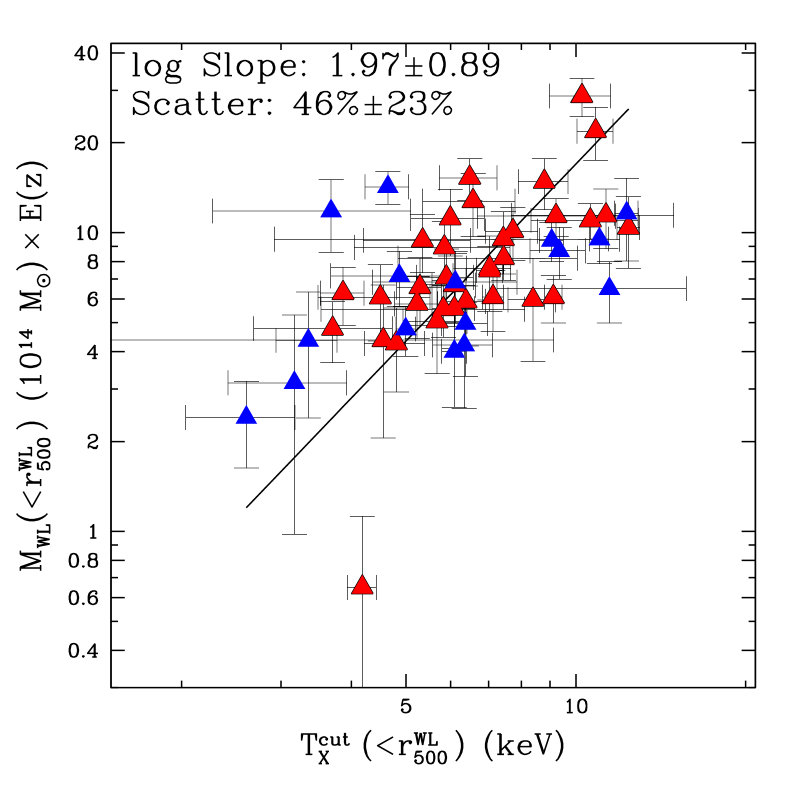
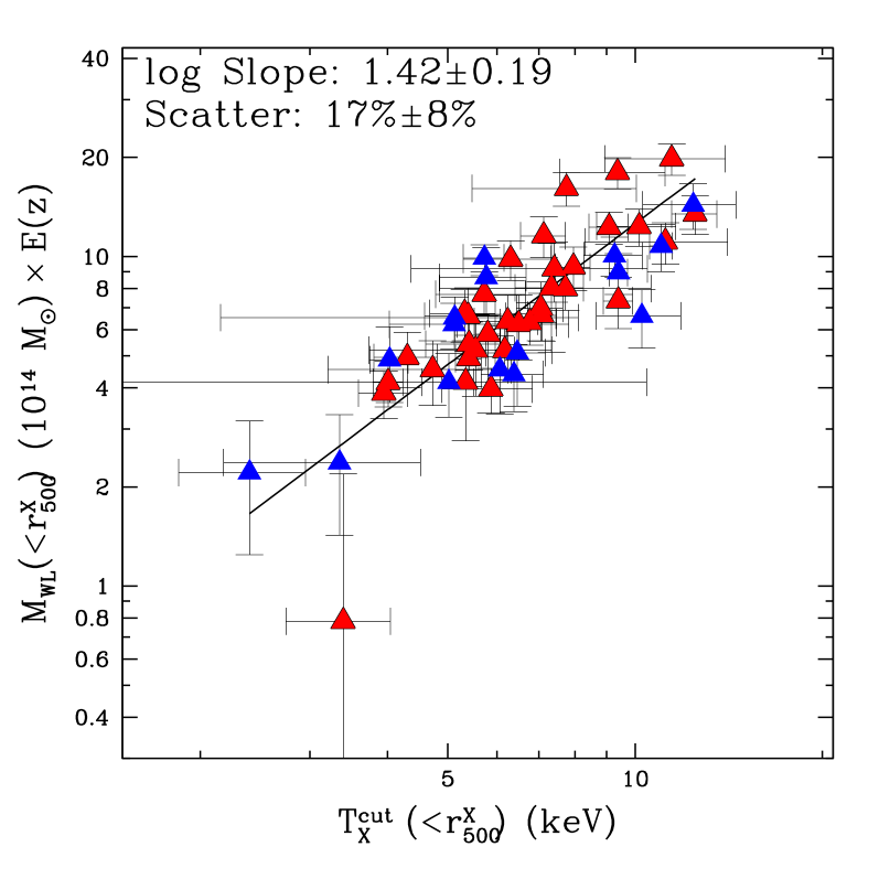
Figure 6.— The mass-temperature relationship at lensing $r_{500}$ (left) and at X-ray $r_{500}$ (right). The latter shows less scatter due to the intrinsic correlation of X-ray $r_{500}$ with temperature. Blue triangles show cool-core clusters and red triangles show non-cool-core clusters.

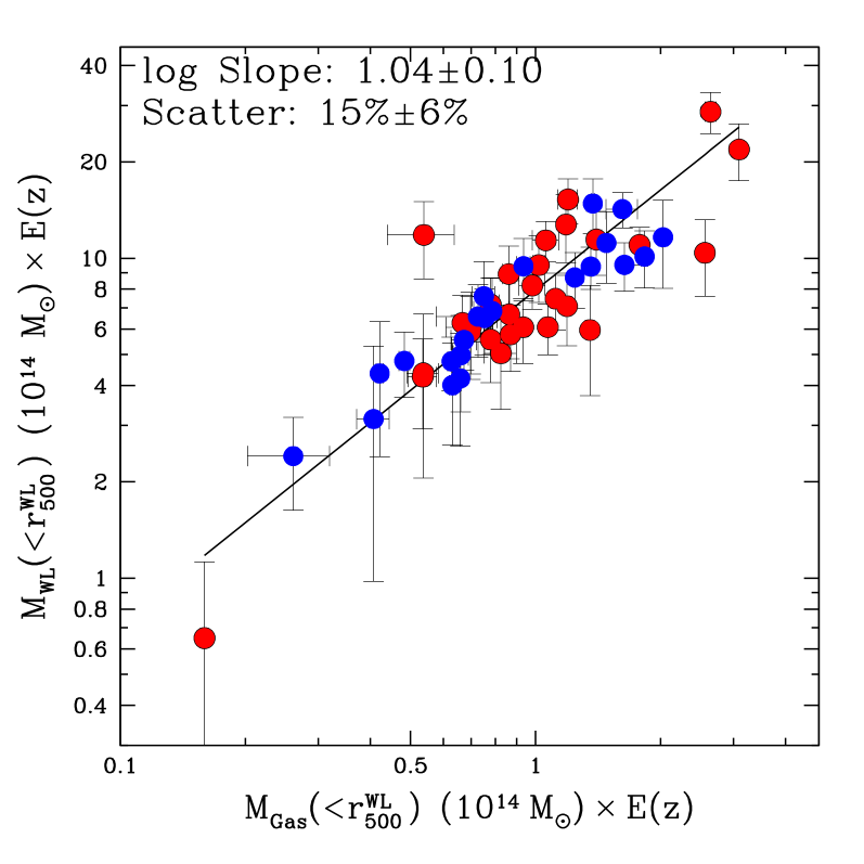
Figure 7.— The gas mass-lensing mass relationship at lensing $r_{500}$. Blue circles show low-BCG-offset systems and red circles show high-BCG-offset systems. Most of the low BCG offset systems are also low central entropy clusters.

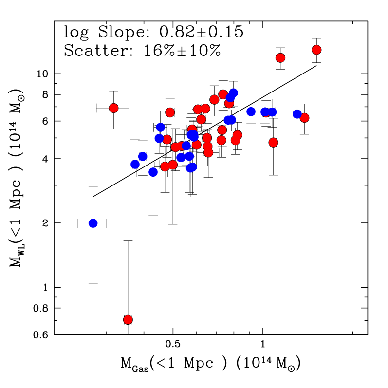
Figure 8.— Lensing mass vs. gas mass at a fixed physical radius of 1 Mpc. Blue circles show low-BCG-offset clusters and red circles show high-BCG-offset clusters. The relation retains the low scatter of the relations at fixed density contrast.

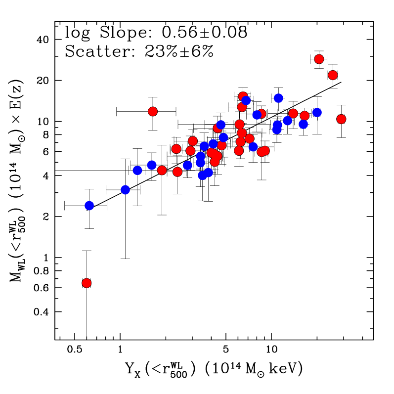
Figure 9.— Lensing mass vs. pseudo-pressure $Y_{X}$. Blue circles show low-BCG-offset clusters and red circles show high-BCG-offset clusters.

t

However, using a physical aperture of 1 Mpc completely takes away any possibility of covariance between the two axes. In Figure 8, we truly have two statistically independent observations, and yet the intrinsic scatter remains remarkably low, $16\%\pm 7\%$. The fact that the scatter does not change when switching to a fixed physical aperture is reassuring. The $1\sigma$ scatter uncertainties are just large enough to accommodate the scatter underestimate predicted by Becker11 (e.g. if the “true” scatter at both $r_{500}^{WL}$ and 1 Mpc is 20%, our $1\sigma$ errors would be consistent with a 50% scatter underestimate at $r_{500}^{WL}$ and no scatter underestimate at 1 Mpc). In Table 3 we also list the performance of $Y_{X}$, $L_{X}$, and $T_{X}$, measured at fixed physical radius of 1 Mpc, as predictors of $M_{WL}(<1$Mpc$)$. Overall, we find little difference between the intrinsic scatter at 1 Mpc compared to $r_{500}^{WL}$.

5.2. Regularity of cool core and low BCG offset clusters

Another point of particular importance is the fact that for the cool-core clusters, the $1\sigma$ scatter is $<10\%$ (the scatter is $<6\%$ if we cut on BCG offset instead)—these numbers are low enough to be consistent with zero. Simulations and analytical work (e.g Becker11) show that $\approx 15\%$ is roughly the amount of intrinsic scatter we can expect due to geometric errors from the assumption of spherical geometry. Thus deviations from spherical symmetry can produce scatter we observe in the cool-core $M_{\mathrm{gas}}-M_{L}$ relation, and as a result, we can begin to claim that we are approaching a full accounting of all sources of systematic error in the mass-observable scaling relation.

We note that the BCG offset works as well as central entropy in identifying the low-scatter subsample. This is an interesting result, because of our four substructure measures, BCG offset is by far the least expensive to calculate, in that it does not require X-ray temperature (spectral) information—a set of X-ray and optical images is sufficient to calculate $D_{\mathrm{BCG}}$. However, it is worth noting that while the low BCG offset and cool-core subsamples have significant overlap, they are not precisely the same, and the two cuts trace two different types of equilibrium (dynamical and thermal, respectively).

Another frequently used mass proxy is $Y_{X}$, the pseudo-integrated pressure first pioneered by Kravtsov06 and examined by Vikhlinin06; being the product of the gas mass and the core-cut temperature at $r_{500}^{WL}$, $Y_{X}$ is directly comparable to the integrated Sunyaev-Zel’dovich compton $Y$ parameter (Plagge10; Andersson11).

We show the $Y_{X}$-$M_{L}$ relation at $r_{500}^{WL}$ for our sample in Figure 9; we find consistency with the expected self-similar slope of 0.6, but slightly higher intrinsic scatter to the gas mass when used as a mass proxy: the overall intrinsic deviation is $\approx 23\%\pm 6\%$ regardless of whether we use the entire sample or the cool-core subsample.

One might be tempted to argue that gas mass is a superior mass proxy to $Y_{X}$, not simply because of its ease of calculation and comparable overall intrisic scatter, but also because of the systematically lower intrinsic scatter that comes about when only cool-core clusters are considered. However, this discrimination between relaxed and non-relaxed clusters is perhaps not optimal in a cosmological context, where uniformity of scatter across the entire sample is important. Where uniformity is most important, $Y_{X}$ is a superior choice to gas mass, because as we show in Table 3 it has uniform scatter regardless of cluster central entropy or BCG offset.

Finally, it is instructive to compare $Y_{X}$ with its radio counterpart, the cylindrically integrated Sunyaev-Zel’dovich (SZ) pressure $Y_{SZ}$. Hoekstra12 consider direct correlations between $Y_{\mathrm{SZ}}$ from the Planck mission and projected weak lensing masses; they find an intrinsic scatter of $12\pm 5\%$ at projected $r_{2500}$. As a point of comparison, when we conduct a similar exercise on spherically determined $Y_{X}$ and $M_{WL}$ (both measured at spherical $r_{2500}^{WL}$), we find an intrinsic scatter of $18\%\pm 6\%$, consistent with the Hoekstra12 SZ comparison.

5.3. Predicting $M_{500}^{WL}$ with fixed aperture mass proxies for surveys

In a blind X-ray survey, the aperture $r_{500}^{WL}$ or even $r_{500}^{X}$ may not be easily available. For cosmology, we still need to know $M_{500}$. It is therefore useful to investigate whether one can directly predict $M_{500}^{WL}$ without the need to calculate overdensity radii $r_{\Delta}$ for the various X-ray observables. For example, a wide-field all-sky X-ray survey may be able to measure hundreds of thousands of gas masses within fixed physical apertures, but lack the photon statistics to allow for the calculation of X-ray overdensity radii.

In Figures 10 we consider this situation, plotting $M_{\mathrm{WL}}(<r_{500}^{WL})$ against gas mass and $Y_{X}$ measured within a fixed radius of $1$ Mpc. As expected, the slopes now deviate from self-similar, and the intrinsic scatter is considerably higher than in Figures 7 and 9. However, interestingly, $Y_{X}$ exhibits somewhat less scatter (29%) in this “mixed” scaling relation than does gas mass (40%). In surveys with poor photon statistics where no X-ray or weak lensing estimates of $r_{500}$ are readily available, $Y_{X}$ measured within a fixed physical aperture may constitute a better mass proxy, because no separate estimate of X-ray $r_{500}$ is required to use the relations shown in Figure 10. The results are summarized in Table 3.

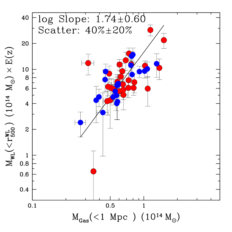
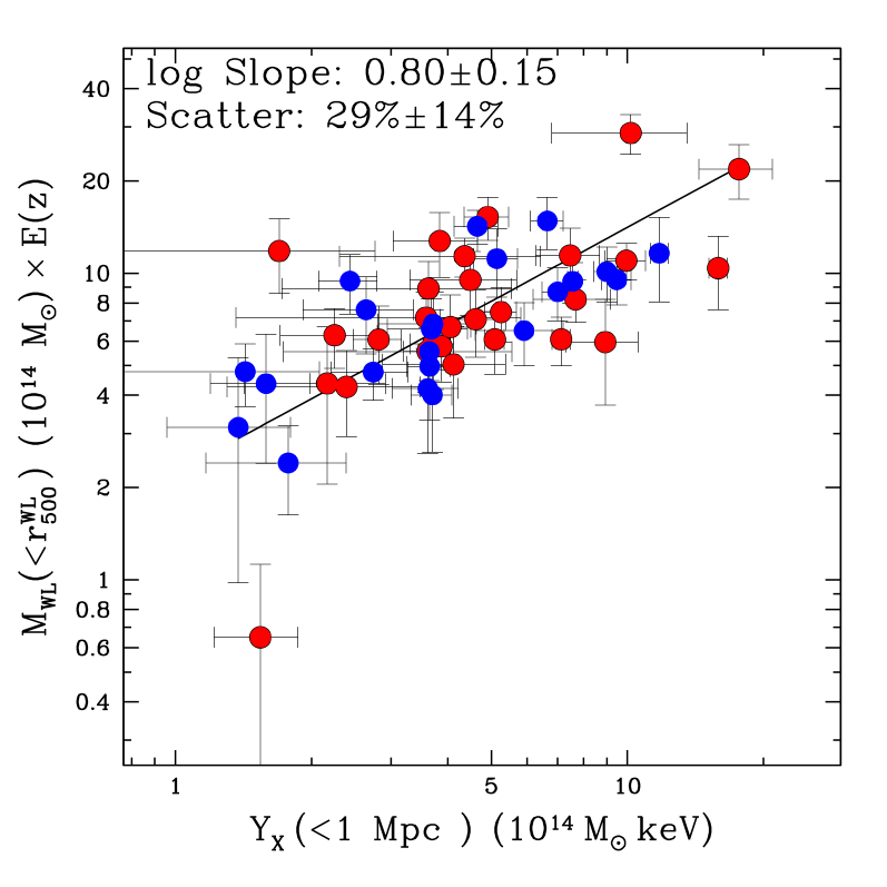
Figure 10.— The lensing mass at $r_{500}$ vs. gas mass and $Y_{X}$ measured at fixed radius of 1 Mpc. Blue circles show low BCG offset clusters, while red circles show high BCG offset clusters.

These data leave us with the perhaps dispiriting result that low ($<10\%$) scatter X-ray mass proxies may be derived either at fixed physical radii, yielding total mass estimates within fixed physical radii; or they may be derived at fixed overdensity radii, yielding total mass estimates within fixed overdensities. But it seems difficult to achieve very low scatter without either committing to fixed physical radii (straightforward to measure, but more difficult to use for cosmology); or to fixed overdensity radii (difficult to measure, but more useful for cosmology) in both axes.

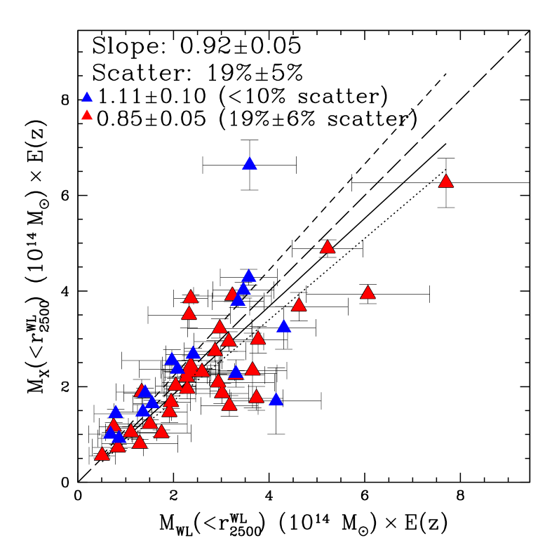
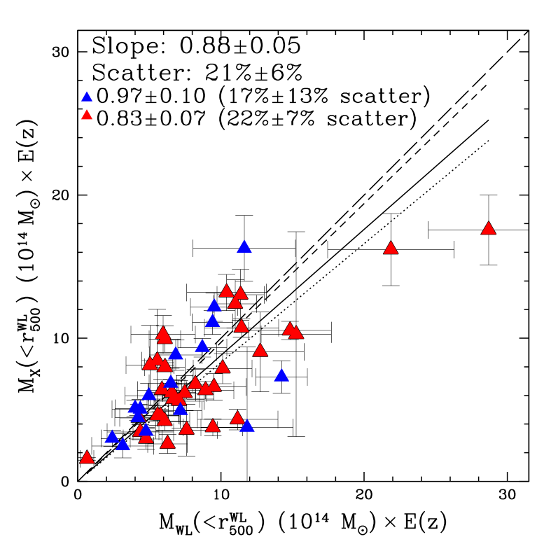
Figure 11.— The relationship between hydrostatic mass and lensing mass at $r_{2500}^{WL}$ (left) and $r_{500}^{WL}$ (right). Blue triangles show cool-core clusters and red triangles show non-cool-core clusters. Cool core clusters tend to have hydrostatic masses that agree with lensing masses; non-cool-core clusters tend to exhibit the hydrostatic mass underestimate. The solid line indicates the best fit; the long-dashed line indicates the line of equality; the short-dashed line corresponds to the cool-core clusters, and the dotted line corresponds to the non-cool-core clusters.

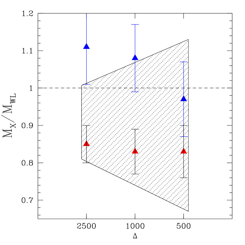
Figure 12.— The X-ray to Weak-Lensing mass ratio as a function of density contrast for cool-core systems (blue triangles) and non-cool-core systems (red triangles). The error bars are not independent because the data within $r_{2500}$ also contributes to the measurement at $r_{500}$. The shaded region shows the range of X-ray cluster mass underestimate as determined by Lau09.

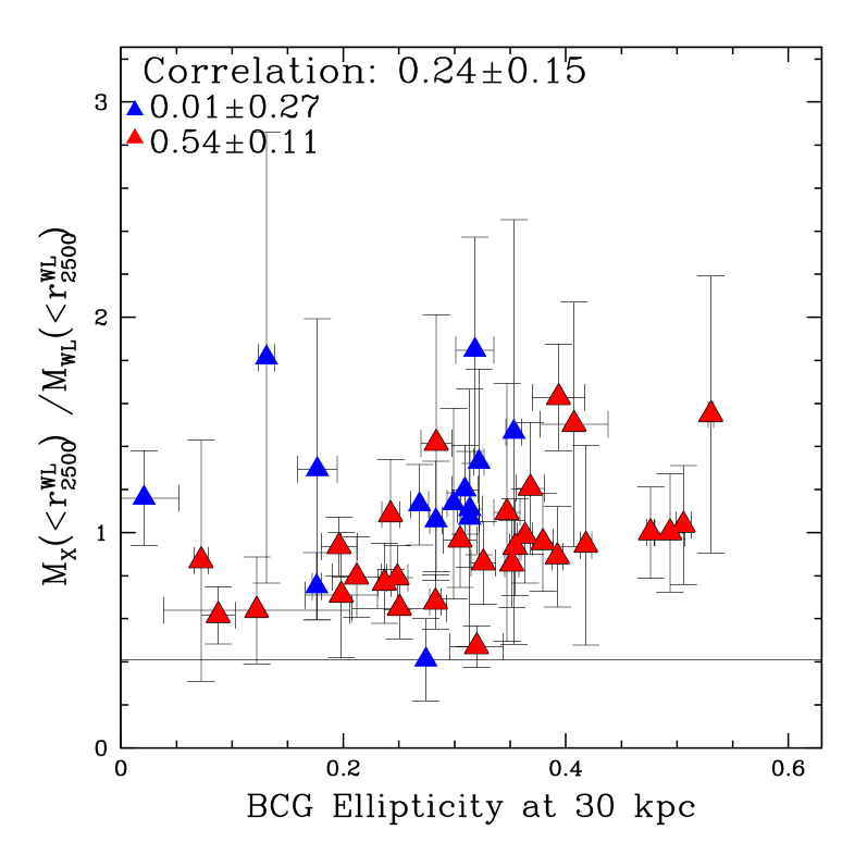
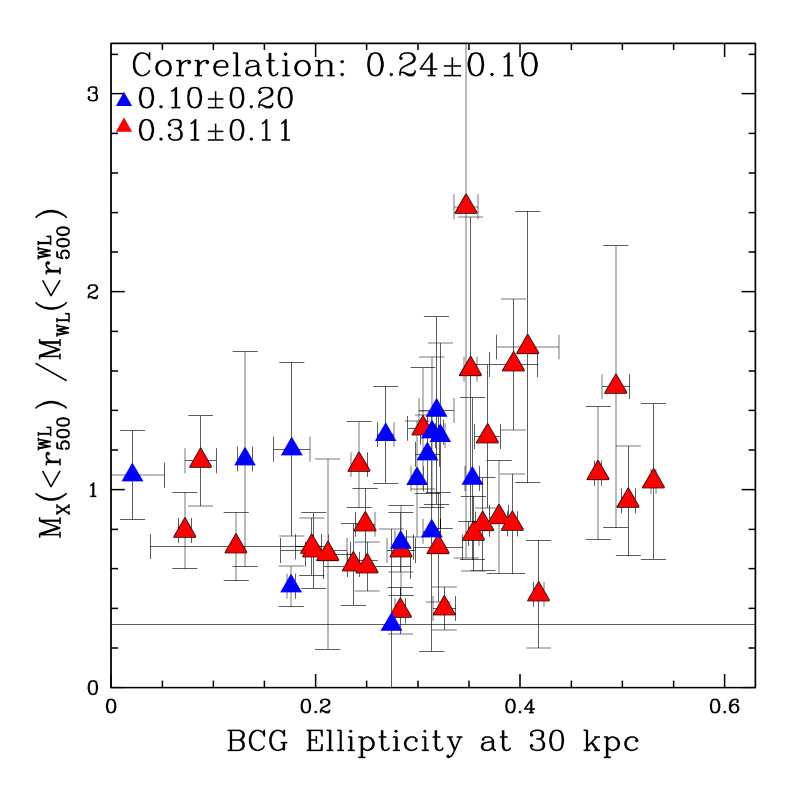
Figure 13.— The X-ray to Weak-Lensing mass ratio as a function of BCG ellipticity for 43 BCGs with measureable ellipticities at 30 kpc. The largest error bar in ellipticity belongs to CL0024. Shown are non-cool-core systems (red triangles) and cool-core systems (blue triangles). The correlation is significant only for the non-cool-core systems at $r_{2500}$; there is a marginal correlation at $r_{500}$. Cool-core systems do not participate in the trend.

5.4. Lack of Correlation with Substructure Measures

We have already argued that the intrinsic scatter in the lensing mass to X-ray observable relations is potentially fully accounted for by the triaxiality of the clusters; nevertheless, it is still useful to consider whether the scatter in such relation may be further minimized via correlation with measures of substructure, at least as an empirical means to gauge the effect of this triaxiality. However, we find that none of the substructure measures—BCG offset, central entropy, centroid shift variance, or power ratio—have any significant correlation with residuals in the mass-observable relation. We note that Marrone12 did find a residual correlation with BCG ellipticity in the relationship between weak lensing mass and the integrated Sunyaev-Zel’dovich effect signal $Y_{\mathrm{SZ}}$. We examine a similar relation in §6.2.

It follows from this lack of correlation that the $M_{x}/M_{WL}$ ratio itself is not correlated with morphological measures such as centroid shift or power ratio, either. Rasia12 consider a similar question; they examine whether the ratio of the X-ray mass to the true mass is correlated with centroid shift or power ratio. They find a weak correlation between this ratio and the substructure measures, with a Pearson rank coefficient of -0.2 to -0.3, significant at $2\sigma$. We do not observe such a correlation, most likely because we do not measure the X-ray to true mass ratio, but rather the X-ray to weak lensing mass ratio, the latter of which has its own intrinsic scatter.

In our present sample, then, it is possible to minimize the scatter in the mass-observable relation by conducting a cut on central entropy, but it is not possible to “correct” this scatter for the non-cool-core clusters by utilizing any of the four substructure quantifiers we consider or even BCG ellipticity.

6. Deviations from Hydrostatic Equilibrium

6.1. Hydrostatic Mass Underestimate

Mahdavi08 argued that a subsample of the clusters discussed here have X-ray masses at $r_{500}^{WL}$ that are on the average $15\%$ lower than their lensing masses at $r_{500}^{WL}$. This discrepancy may be attributed to deviations from hydrostatic equilibrium due to residual gas motions and incomplete thermalization of the ICM; the fact that hydrostatic masses tend to underestimate the true mass by 10-20% was first discussed by Evrard90 and continues to be important in grid-based simulations (e.g. Lau09; Nelson12), SPH simulations (e.g. Rasia06; Battaglia12; Rasia12), and observations of distant clusters (Andersson11; Jee11). Biases in gravitational lensing masses could in principle also affect the X-ray to weak-lensing mass ratio, such systematic biases are only $\approx 5-10\%$, but would have the effect of increasing the X-ray to weak lensing mass ratio (e.g. Becker11). Note that in recent N-body hydrodynamical simulations, even though the hydrostatic bias (10-15%) is roughly twice the level of the weak lensing bias, the scatter about this bias is larger by a factor of two for weak lensing masses than for the hydrostatic masses (Meneghetti10; Rasia12; Nelson12).

It is worth pointing out, however, that the technique we use for our lensing mass measurements should yield lower bias than suggested by these simulations. The technique achieves this lower bias of 3-4% (rather than the expected bias of 5-10%) by omitting the regions of the shear map that are most susceptible, at the cost of increased statistical uncertainty. We refer the reader to Hoekstra12 for details.

In Figure 11 we extend our results to the full sample of 50 clusters. The larger size of the sample allows us to resolve differences between cool-core and non-cool core clusters. We find that cool-core clusters and non-cool-core clusters do not exhibit the same level of departure from hydrostatic equilibrium.

Cool core clusters have hydrostatic masses that are proportional to their weak lensing masses at all radii. The $M_{X}-M_{L}$ relation for this subsample has a small scatter ($<20\%$), about the right level for all the scatter to be accounted for by triaxiality. Overall, we find that cool core clusters are consistent with having no difference between their X-ray and weak lensing masses.

The picture is dramatically different for non-cool-core clusters. In these systems, we find a roughly constant hydrostatic mass to lensing mass ratio of $80\%$, regardless of whether we look at $r_{500}^{WL}$ or $r_{2500}^{WL}$. Our results are consistent with N-body gas dynamical simulations as shown in Figure 12 and Table 6.2. Broadly, these results are consistent the hydrostatic mass underestimates predicted by gasdynamical simulations that account for unthermalized gas, such as Nagai07, Jeltema08 and Lau09. We find that the non-cool-core clusters populate the lower end of the region allowed by these simulations, whereas the cool-core clusters populate the region where X-ray and true mass agree within 10%. Of these simulations Jeltema08 is the most consistent with our measured $20\%$ average mass underestimate for disturbed systems.

6.2. Correlation with BCG Ellipticity

Finally, we consider the question of whether BCG ellipticity is correlated with differences between hydrostatic and weak lensing masses. Such a correlation is suggested by Marrone12, who use the integrated Compton parameter $Y_{\mathrm{sph}}$ as a mass proxy. In figure 13, we show $M_{X}/M_{\mathrm{WL}}$ at $r_{2500}$ and $r_{500}$, plotted against CFHT ellipticities measured at 30kpc. We find that cool-core systems are consistent with $M_{X}/M_{L}=1$ $(\chi^{2}/\nu=18/14)$; whereas non-cool-core systems are definitively not consistent with $M_{x}/M_{L}=1$ ($\chi^{2}/\nu=70/29$).

Therefore, for non-cool-core systems, we find a good correlation between BCG ellipticity and the X-ray to weak lensing ratio ratio at $r_{2500}^{WL}$, and a weak correlation at $r_{500}$. While this is similar to the trend found by Marrone12 for $Y_{\mathrm{sph}}$, there is a difference in that our cool-core systems do not appear to participate in the correlation. Furthermore, also in apparent contrast with Marrone12, our correlation becomes less significant at $r_{500}^{WL}$. We interpret this result as suggesting that while cluster orientation plays some role in low X-ray to weak lensing mass ratios, it is not the only agent at work in this complex relationship (indeed, the hydrostatic mass underestimate must also play a role).

We note that it is not altogether surprising that the trend of ellipticity with $M_{X}/M_{L}$ for cool core clusters is insignificant. We have shown in §6 that our X-ray and weak-lensing masses are consistent for this sub-population (in contrast, Marrone12 contained several undisturbed clusters with significant $Y_{\mathrm{sph}}$ to weak lensing mass discrepancies).

Furthermore, it is difficult to untangle the effects of elongation along the line of sight (which would chiefly bias weak lensing masses high) and non-hydrostatic gas (which would chiefly bias the X-ray masses low). We also stress that the trend is altogether absent at $r_{500}$ However, empirically, we can point out that the non-cool-core clusters with the highest ellipticities have consistent X-ray and weak lensing masses, something corroborated by Marrone12.

Table 3Mass Proxy Fits with Lognormal Intrinsic Scatter

	Proxy	$M_{WL}$		Log	Log	Fractional Scatter
Proxy	Aperture	Aperture	Sample	Slope	Intercept	in $M_{WL}$ at fixed proxy
Relations at Fixed Overdensity in Proxy and Mass
$T^{cut}_{X}/8$ keV	$r_{500}^{WL}$	$r_{500}^{WL}$	all	$1.97\pm 0.89$	$1.04\pm 0.06$	$0.46\pm 0.23$
$T^{cut}_{X}/8$ keV	$r_{500}^{X}$	$r_{500}^{X}$	all	$1.42\pm 0.19$	$0.96\pm 0.02$	$0.17\pm 0.08$
$L^{cut}_{X}E(z)^{-1}$	$r_{500}^{WL}$	$r_{500}^{WL}$	all	$0.45\pm 0.10$	$0.93\pm 0.03$	$0.35\pm 0.07$
$L^{cut}_{X}E(z)^{-1}$	$r_{500}^{X}$	$r_{500}^{X}$	all	$0.50\pm 0.06$	$0.91\pm 0.02$	$0.26\pm 0.05$
$M_{\mathrm{Gas}}E(z)$	$r_{500}^{WL}$	$r_{500}^{WL}$	all	$1.04\pm 0.10$	$0.90\pm 0.02$	$0.15\pm 0.06$
			$K_{0}<70$ keV cm2	$0.91\pm 0.20$	$0.89\pm 0.03$	$<0.1$
			$K_{0}>70$ keV cm2	$1.09\pm 0.13$	$0.90\pm 0.02$	$0.18\pm 0.09$
			$D_{\mathrm{BCG}}<$ 0.01 Mpc	$0.93\pm 0.13$	$0.89\pm 0.02$	$<0.06$
			$D_{\mathrm{BCG}}>$0.01 Mpc	$1.13\pm 0.18$	$0.90\pm 0.03$	$0.22\pm 0.15$
$Y_{X}E(z)^{0.6}$	$r_{500}^{WL}$	$r_{500}^{WL}$	all	$0.56\pm 0.07$	$0.45\pm 0.07$	$0.22\pm 0.05$
			$K_{0}<70$ keV cm2	$0.44\pm 0.14$	$0.53\pm 0.11$	$0.24\pm 0.18$
			$K_{0}>70$ keV cm2	$0.62\pm 0.10$	$0.41\pm 0.09$	$0.21\pm 0.09$
			$D_{\mathrm{BCG}}<$ 0.01	$0.48\pm 0.09$	$0.52\pm 0.08$	$0.17\pm 0.11$
			$D_{\mathrm{BCG}}>$0.01	$0.65\pm 0.14$	$0.36\pm 0.13$	$0.27\pm 0.17$
Relations at Other Radii
$T^{cut}_{X}$/8 keV (keV)	1 Mpc	1 Mpc	all	$1.10\pm 0.57$	$0.80\pm 0.02$	$0.15\pm 0.11$
$L^{cut}_{X}$	”	”	all	$0.23\pm 0.06$	$0.79\pm 0.02$	$0.19\pm 0.04$
$M_{Gas}$	”	”	all	$0.83\pm 0.14$	$0.90\pm 0.03$	$0.16\pm 0.10$
$Y_{X}$	”	”	all	$0.40\pm 0.06$	$0.48\pm 0.05$	$0.12\pm 0.04$
$T^{cut}_{X}$/8 keV	”	$r_{500}^{WL}$	all	$3.04\pm 1.38$	$1.03\pm 0.08$	$0.46\pm 0.31$
$L^{cut}_{X}$	”	$r_{500}^{WL}$	all	$0.50\pm 0.13$	$0.96\pm 0.03$	$0.38\pm 0.07$
$M_{Gas}$	”	$r_{500}^{WL}$	all	$1.73\pm 0.59$	$1.20\pm 0.13$	$0.39\pm 0.18$
$Y_{X}$	”	$r_{500}^{WL}$	all	$0.80\pm 0.15$	$0.35\pm 0.11$	$0.28\pm 0.14$

Note. — All proxies are fit against $M_{WL}E(z)$ at an aperture of $r_{500}^{WL}$ or $M_{WL}$ at an aperture of 1 Mpc. All masses are in units of $10^{14}M_{\odot}$. The core-cut X-ray luminosity is in units of $10^{45}$ erg s^-1, and $Y_{X}$ is in units of $10^{14}M_{\odot}$ keV.

Table 4X-ray to Weak Lensing Mass Ratios

Contrast	Sample	$M_{X}/M_{L}$	Fractional Scatter
			in $M_{X}$ at fixed $M_{L}$
$r_{2500}^{\mathrm{WL}}$	All	$0.92\pm 0.05$	$0.19\pm 0.05$
	$K_{0}<70$ keV cm2	$1.11\pm 0.10$	$<10\%$
	$K_{0}>70$ keV cm2	$0.85\pm 0.05$	$0.19\pm 0.06$
	$D_{\mathrm{BCG}}<0.01$ Mpc	$1.04\pm 0.07$	$<0.15$
	$D_{\mathrm{BCG}}>0.01$ Mpc	$0.81\pm 0.07$	$0.24\pm 0.07$
$r_{1000}^{\mathrm{WL}}$	All	$0.89\pm 0.05$	$0.20\pm 0.05$
	$K_{0}<70$ keV cm2	$1.08\pm 0.09$	$<9\%$
	$K_{0}>70$ keV cm2	$0.83\pm 0.06$	$0.20\pm 0.06$
	$D_{\mathrm{BCG}}<0.01$ Mpc	$0.97\pm 0.07$	$0.13\pm 0.10$
	$D_{\mathrm{BCG}}>0.01$ Mpc	$0.84\pm 0.06$	$0.22\pm 0.07$
$r_{500}^{\mathrm{WL}}$	All	$0.88\pm 0.05$	$0.21\pm 0.06$
	$K_{0}<70$ keV cm2	$0.97\pm 0.10$	$0.17\pm 0.13$
	$K_{0}>70$ keV cm2	$0.83\pm 0.07$	$0.22\pm 0.07$
	$D_{\mathrm{BCG}}<0.01$ Mpc	$0.85\pm 0.09$	$0.22\pm 0.11$
	$D_{\mathrm{BCG}}>0.01$ Mpc	$0.89\pm 0.07$	$0.20\pm 0.08$