The FSI contribution to the observed $B_{s}$ decays into $K^{+}K^{-}$ and $\pi^{+}K^{-}$

Abstract

Because at the tree level $B_{s}\rightarrow K^{+}K^{-}$ is Cabibbo-triple suppressed, so its branching ratio should be smaller than that of $B_{s}\to\pi^{+}K^{-}$. The measurements present a reversed ratio as $R=\mathcal{B}(B_{s}\rightarrow\pi^{+}K^{-})/\mathcal{B}(B_{s}\rightarrow K^{+}K^{-})\sim{4.9/33}$. Therefore, It has been suggested that the transition $B_{s}\to K^{+}K^{-}$ is dominated by the penguin mechanism, which is proportional to $V_{cb}V^{*}_{cs}$. In this work, we show that an extra contribution from the final state interaction (FSI) to $B_{s}\to K^{+}K^{-}$ via sequential processes $B_{s}\to D^{(*)}_{(s)}\bar{D}_{s}^{(*)}\to K^{+}K^{-}$ is also substantial and should be superposed on the penguin contribution. Indeed, taking into account of the FSI effects, the theoretical prediction on $R$ is well consistent with the data.

I Introduction

It is generally believed that the hierarchy of the Cabibbo-Kabayashi-Maskawa (CKM) matrix elements determines the magnitudes of weak decays, and off-diagonal matrix elements would bring up an order suppression. For example, the ratio of $\mathcal{B}(B_{s}\rightarrow D_{s}^{+}\pi^{-})/\mathcal{B}(B_{s}\rightarrow D_{s}^{\pm}K^{\mp})=3.2\times 10^{-3}/3.0\times 10^{-4}$ has been measured Abulencia:2006aa ; Louvot:2008sc , and it is roughly determined by the ratio of the CKM matrix elements $V_{ud}/V_{us}$. Thus one usually categorizes the weak decays according to their CKM structures as the Cabibbo-favored; Cabibbo-suppressed and even the Cabibbo-double or triple-suppressed. However, the newly observed modes $B_{s}\rightarrow K^{+}K^{-}$ and $B_{s}\rightarrow\pi^{+}K^{-}$ obviously do not follow the rule, namely at first look, the branching ratio of $B_{s}\rightarrow K^{+}K^{-}$ should be smaller than that of $B_{s}\rightarrow\pi^{+}K^{-}$ by $|V_{us}/V_{ud}|^{2}$, by contraries, the datum is $\mathcal{R}=\mathcal{B}(B_{s}\rightarrow\pi^{+}K^{-})/\mathcal{B}(B_{s}\rightarrow K^{+}K^{-})={4.9}\times 10^{-6}/3.3\times 10^{-5}$ PDG10 ; Abulencia:2006psa ; Aaltonen:2008hg . If only the tree diagrams are taken into account, this reversion would compose an “anomaly”. Descotes-Genon et al. DescotesGenon:2006wc carefully analyzed the transitions of $B_{s}\to K^{0}\bar{K}^{0}$ and $K^{+}K^{-}$ through flavor symmetries and QCD factorization, and pointed a potential conflict between the QCD prediction on $B_{s}\to K^{+}K^{-}$ and data. By analyzing the transition mechanism, Cheng and Chua Cheng determined that the main contribution to $B_{s}\to K^{+}K^{-}$ comes from the penguin diagram, which is proportional to $V_{cb}V^{*}_{cs}$. Ali et al. also calculated the branching ratios of $B_{s}\to\pi^{+}K^{-}$ and $B_{s}\to K^{+}K^{-}$ in terms of the Perturbative QCD (PQCD) to LO and NLO Ali:2007ff ; Liu:2008rz and the authors of Ref. Williamson:2006hb did calculations in SCET. Their results roughly were consistent with the data available then, so the “conflict” seemed resolved. Even though the theoretical uncertainties in all the calculations are not fully controlled, it is noted that the obtained central values are not sufficiently large to make up the data. It implies that there must be some mechanisms to remarkably enhance the branching ratio of $B_{s}\rightarrow K^{+}K^{-}$.

Looking at the central values they obtained and the resultant ratio of $\mathcal{B}(B_{s}\to\pi^{+}K^{-})/\mathcal{B}(B_{s}\to K^{+}K^{-})$, one can find that the calculated $\mathcal{B}(B_{s}\to\pi^{+}K^{-})$ is close to the data, however, the central values of $\mathcal{B}(B_{s}\to K^{+}K^{-})$ calculated in various approaches are smaller than the newly measured data Abulencia:2006psa ; Aaltonen:2008hg .

Based on this observation, we suggest that the final state interaction (FSI) in $B_{s}$ decays may greatly enhance the branching ratio of $B_{s}\to K^{+}K^{-}$ but not much for $B_{s}\to\pi^{+}K^{-}$. In fact, in the energy regions of $b$-quark and $c$-quark most such anomalies can be naturally explained by considering the role of FSI. For example, a simple quark diagram-analysis tells that the branching ratio of $D^{0}\to K^{0}\bar{K}^{0}$ is almost zero, but its measured value is comparable with that of $D^{0}\to K^{+}K^{-}$, which is large. This can be understood by considering the sequential process $D^{0}\to K^{+}K^{-}\to K^{0}\bar{K}^{0}$ and the later step is a hadronic scattering Dai:1999cs .

The Particle Data Group (PDG) PDG10 tells us that the $D_{s}^{(*)+}D_{s}^{(*)-}$ are the dominant hadronic decay modes of $B_{s}$, therefore it implies that the sequential decays $B_{s}\to D_{s}^{(*)+}D_{s}^{(*)-}\to K^{+}K^{-}$ would compose an important contribution to the observed $B_{s}\to K^{+}K^{-}$. The first step of $B_{s}\to D_{s}^{(*)+}D_{s}^{(*)-}$ is only suppressed by $V_{bc}$ and the process does not suffer form a color-suppression. Moreover it is also isospin-conserved mode, even though the weak interaction does not require isospin conservation, it still may be more favorable than the isospin violated ones. Thus, one can understand why $B_{s}\to D_{s}^{(*)+}D_{s}^{(*)-}$ is dominant. Then let us look at the next step. The FSI is a hadronic scattering process, which is completely governed by strong interaction, so that the isospin must be conserved. The isospin of $D_{s}^{(*)\pm}$ is zero, thus, the final state of the scattering is required to be zero. The isospin of $K$-mesons is 1/2, thus the $K\bar{K}$-states can be either isospin 0 or 1, therefore the inelastic scattering $D_{s}^{(*)+}D_{s}^{(*)-}\to K^{+}K^{-}$ is allowed. By contraries, isospin of pion is 1, thus, the system of $\pi^{+}K^{-}$ does not contain an isospin 0 component, thus the scattering $D_{s}^{(*)+}D_{s}^{(*)-}\to\pi^{+}K^{-}$ is forbidden. Definitely, one can expect a substantial contribution from $B_{s}\to D_{s}^{(*)+}D_{s}^{(*)-}\to K^{+}K^{-}$, which can much enhance the branching ratio of $B_{s}\to K^{+}K^{-}$ in comparison with $B_{s}\to\pi^{+}K^{-}$.

It is worth pointing out that on the other hand, the decay $B_{s}\rightarrow\pi^{+}K^{-}$ also receives a contribution from the FSI via $B_{s}\rightarrow D^{(*)+}D_{s}^{(*)-}\rightarrow\pi^{+}K^{-}$. However, the first step process $B_{s}\rightarrow D^{(*)+}D_{s}^{(*)-}$ is Cabibbo-double suppressed by $V_{cb}V_{cd}^{*}$, so is much less than $B_{s}\rightarrow D_{s}^{(*)+}D_{s}^{(*)-}$, therefore the FSI does not contribute much to the branching ratio of $B_{s}\rightarrow\pi^{+}K^{-}$.

Notice that, the direct process $B_{s}\to K^{+}K^{-}$ via penguin diagrams and the sequential process with FSI $B_{s}\rightarrow D_{s}^{(*)}D_{s}^{(*)}\rightarrow K^{+}K^{-}$ have the same initial and final states, moreover their amplitudes are of the same order of magnitude, so the two contributions interfere. In fact, their contributions are not directly experimentally, but theoretically distinguishable. Moreover, the strong scattering would have a real and an imaginary parts (see below, for the calculations of the triangle diagrams), thus a phase is resulted. In most calculations of the FSI effects, only the absorptive (imaginary) part is kept, the reason is that one may argue that the absorptive part might be dominant or at most the dispersive and absorptive parts have close magnitudes. In that case, the absorptive part is imaginary while the penguin contribution is real, so that the two contributions can be added up at the rate level (amplitude square). Our final results indicate that while taking into account the new contribution, the theoretical predictions are indeed close to the new data.

In this work, we calculate the amplitudes of the decay channels of $B_{s}\rightarrow D_{s}^{(*)}(D^{(*)})\bar{D}_{s}^{(*)}$ and the direct decay channels of $B_{s}\rightarrow K^{+}(\pi^{+})K^{-}$ by the factorization approach Matinyan:1998cb ; Ablikim:2002ep . Then we use the effective SU(4) Lagrangian Haglin:1999xs ; Lin:1999ad to determine the vector-pseudoscalar-pseudoscalar and vector-vector-pseudoscalar vertices for calculating the FSI amplitude of $D_{s}^{(*)}(D^{(*)})\bar{D}_{s}^{(*)}\rightarrow K^{+}(\pi^{+})K^{-}$. The paper is organized as follows, after the introduction, we formulate the weak decays and the re-scattering processes in section II, our numerical results are presented along with all necessary inputs in section III. The last section is devoted to discussion and conclusion.

II The theoretical evaluations of the branching ratios

II.1 Weak decays in factorization approach

Because the measurements on the decay widths of $B_{s}\to D_{s}^{(*)+}D_{s}^{(*)-}$ and $B_{s}\to D^{(*)+}D_{s}^{(*)-}(B_{s}\to D^{(*)-}D_{s}^{(*)+})$ are not accurate yet, as for most of the above channels there are only upper bounds, so that we are going to directly calculate the transition amplitudes based on the quark diagrams. Even though this strategy might bring up certain theoretical uncertainties, it does not break our qualitative conclusion at all.

For calculating the transition amplitudes of $B_{s}\rightarrow D_{s}^{(*)+}(D^{(*)+})D_{s}^{(*)-}$, one needs to employ the effective hamiltonian at the quark level. With the operator product expansion (OPE), the effective Hamiltonian was explicitly presented in Ref. Buchalla:1995vs . At the tree level, from the effective Lagrangian one can notice that $B_{s}\to K^{+}K^{-}$ is suppressed by $V_{ub}V^{*}_{us}$ i.e triple-Cabibbo suppressed, comparing with $B_{s}\to\pi^{+}K^{-}$, which is double-Cabibbo suppressed by $V_{ub}$. Therefore Cheng and Chua decided that the direct transition $B_{s}\to K^{+}K^{-}$ is obviously dominated by the penguin diagram whose CKM structure is $V_{cb}V^{*}_{cs}$. The transition $B_{s}\to D^{(*)+}_{s}D^{(*)-}$ is also double-Cabibbo suppressed. Instead, $B_{s}\to D^{(*)+}_{s}D^{(*)-}_{s}$ is proportional to $V_{cb}V^{*}_{cs}$ and it is a tree process. Now let us compare the sequential processes $B_{s}\to D^{(*)}\bar{D}_{s}^{(*)}\to K^{+}K^{-}$ with the penguin contribution. The two reactions are of the same CKM structure, but the penguin undergoes a loop suppression about $\alpha_{s}/\pi\sim 0.06$, whereas the strong scattering $D_{s}^{(*)}\bar{D}_{s}^{(*)}\to\sum_{i}X_{i}$ where $X_{i}$ stands as any possible final states allowed by symmetry and energy-momentum conservation. $K^{+}K^{-}$ is only one of the possible channels, and its probability is proportional to $\langle D_{s}^{(*)}\bar{D}_{s}^{(*)}|H_{eff}|K\bar{K}\rangle$, which is what we are going to calculate in this work. This is a suppression factor because the total probability to all channels is 1. Therefor, roughly, we notice that the penguin is loop-suppressed and the sequential process is also suppressed by the probability, thus the two modes compete and may have a similar order of magnitude. Concretely, we need to calculate them. The explicit calculation on the penguin contribution can be found in Ali:2007ff ; Liu:2008rz ; Cheng , thus we will use their numbers and only consider the contribution from the sequential processes.

Applying the effective hamiltonian at the quark level to the hadron states, the hadronic matrix elements can be parameterized as Cheng:2003sm :

$$\langle 0|J_{\mu}|P(p_{1})\rangle = -if_{P}p_{1\mu},$$

$$\langle 0|J_{\mu}|V(p_{1},\epsilon)\rangle = f_{V}\epsilon_{\mu}m_{V},$$

$$\langle P(p_{2})|J_{\mu}|B_{s}(p)\rangle = \Big{[}P_{\mu}-{m_{B_{s}}^{2}-m_{P}^{2}\over q^{2}}q_{\mu}\Big{]}F_{1}(q^{2})+{m_{B_{s}}^{2}-m_{P}^{2}\over q^{2}}q_{\mu}F_{0}(q^{2}),$$

$$\langle V(p_{2},\epsilon)|J_{\mu}|B_{s}(p)\rangle = {i\epsilon^{\nu}\over m_{B_{s}}+m_{V}}\Big{\{}i\epsilon_{\mu\nu\alpha\beta}P^{\alpha}q^{\beta}A_{V}(q^{2})+(m_{B_{s}}+m_{V})^{2}g_{\mu\nu}A_{1}(q^{2})-{P_{\mu}P_{\nu}\over m_{B_{s}}+m_{V}}A_{2}(q^{2})$$ (1)

$$-2m_{V}(m_{B_{s}}+m_{V}){P_{\nu}q_{\mu}\over q^{2}}[A_{3}(q^{2})-A_{0}(q^{2})]\Big{\}},$$

where $J_{\mu}=\bar{q}_{1}\gamma_{\mu}(1-\gamma_{5})q_{2}$, $P_{\mu}=(p_{1}+p_{2})_{\mu}$ and $q_{\mu}=(p_{1}-p_{2})_{\mu}$.

With Eq. (II.1), we write down the amplitudes of $B_{s}\rightarrow D_{s}^{(*)+}D_{s}^{(*)-}$:

$$\mathcal{A}(B_{s}(p)\rightarrow D_{s}^{+}(p_{1})D_{s}^{-}(p_{2})) = -{iG_{F}\over\sqrt{2}}V_{cb}V^{*}_{cs}a_{1}f_{D_{s}}(m_{B_{s}}^{2}-m_{D_{s}}^{2})F_{0}^{B_{s}D_{s}}(p_{1}^{2}),$$ (2a)

$$\mathcal{A}(B_{s}(p)\rightarrow D^{*+}_{s}(p_{1})D^{*-}_{s}(p_{2})) = {G_{F}\over\sqrt{2}}V_{cb}V^{*}_{cs}a_{1}f_{D_{s}^{*}}m_{D_{s}^{*}}{ig^{\mu\nu}\over m_{B_{s}}+m_{D_{s}^{*}}}\Big{\{}i\epsilon_{\mu\nu\alpha\beta}(p_{1}+2p_{2})^{\alpha}p_{1}^{\beta}A_{V}^{B_{s}D_{s}^{*}}(p_{1}^{2})+(m_{B_{s}}$$

$$+m_{D_{s}^{*}})^{2}g_{\mu\nu}A_{1}^{B_{s}D_{s}^{*}}(p_{1}^{2})-(p_{1}+2p_{2})_{\mu}(p_{1}+2p_{2})_{\nu}A_{2}^{B_{s}D_{s}^{*}}(p_{1}^{2})-{(p_{1}+2p_{2})_{\mu}p_{1\nu}\over p_{1}^{2}}\Big{[}(m_{B_{s}}$$

$$+m_{D^{*}_{s}})^{2}A_{1}^{B_{s}D_{s}^{*}}(p_{1}^{2})-(m_{B_{s}}^{2}-m_{D^{*}_{s}}^{2})A_{2}^{B_{s}D_{s}^{*}}(p_{1}^{2})-2m_{D^{*}_{s}}(m_{B_{s}}+m_{D^{*}_{s}})A_{0}^{B_{s}D_{s}^{*}}(p_{1}^{2})\Big{]}\Big{\}},$$

and the amplitudes of $$B_{s}\rightarrow D^{(*)+}D_{s}^{(*)-}$$ read as

$$\mathcal{A}(B_{s}(p)\rightarrow D^{+}(p_{1})D_{s}^{-}(p_{2})) = -{iG_{F}\over\sqrt{2}}V_{cb}V^{*}_{cd}a_{1}f_{D}(m_{B_{s}}^{2}-m_{D_{s}}^{2})F_{0}^{B_{s}D_{s}}(p_{1}^{2}),$$ (2c)

$$\mathcal{A}(B_{s}(p)\rightarrow D^{*+}(p_{1})D_{s}^{*-}(p_{2})) = {G_{F}\over\sqrt{2}}V_{cb}V^{*}_{cd}a_{1}f_{D^{*}}m_{D^{*}}{ig^{\mu\nu}\over m_{B_{s}}+m_{D_{s}^{*}}}\Big{\{}i\epsilon_{\mu\nu\alpha\beta}(p_{1}+2p_{2})^{\alpha}p_{1}^{\beta}A_{V}^{B_{s}D_{s}^{*}}(p_{1}^{2})+(m_{B_{s}}$$

$$+m_{D_{s}^{*}})^{2}g_{\mu\nu}A_{1}^{B_{s}D_{s}^{*}}(p_{1}^{2})-(p_{1}+2p_{2})_{\mu}(p_{1}+2p_{2})_{\nu}A_{2}^{B_{s}D_{s}^{*}}(p_{1}^{2})-{(p_{1}+2p_{2})_{\mu}p_{1\nu}\over p_{1}^{2}}\Big{[}(m_{B_{s}}$$

$$+m_{D^{*}_{s}})^{2}A_{1}^{B_{s}D_{s}^{*}}(p_{1}^{2})-(m_{B_{s}}^{2}-m_{D^{*}_{s}}^{2})A_{2}^{B_{s}D_{s}^{*}}(p_{1}^{2})-2m_{D^{*}_{s}}(m_{B_{s}}+m_{D^{*}_{s}})A_{0}^{B_{s}D_{s}^{*}}(p_{1}^{2})\Big{]}\Big{\}},$$

the amplitude of $$\pi^{+}K^{-}$$ at the tree level is:

$$\mathcal{A}^{\mathrm{direct}}(B_{s}(p)\rightarrow\pi^{+}(p_{1})K^{-}(p_{2})) = -{iG_{F}\over\sqrt{2}}V_{ub}V^{*}_{ud}a_{1}f_{\pi}(m_{B_{s}}^{2}-m_{K}^{2})F_{0}^{B_{s}K}(p_{1}^{2}),$$ (2e)

where $a_{1}$ is a proper combination of the Wilson coefficients in the effective hamiltonian Buchalla:1995vs ; Cheng:1986an ; Li:1988hr . $F_{0}(q^{2})$ and $A_{V,1,2}(q^{2})$ are the form factors to be detrmined. In this work, due to lack of accurate data, we use the form factors obtained by fitting the data of the decays of $B$ meson. It is a reasonable approximation because the processes $B_{s}\rightarrow D_{s}^{*}$ and $B\rightarrow D^{*}$ have the same topological structure, and the flavor $SU(3)$ symmetry for light quarks ($u$, $d$ and $s$) would lead to the same form factors, namely the difference between the form factors for different light-quark flavors would be proportional to an $SU(3)$ breaking, which is small for the effective vertices as well known. At least such small difference would not overtake the errors caused by experimental measurements and theoretical uncertainties for evaluating the non-perturbtive effects.

Moreover, a symmetry analysis indicates that the sequential process $B_{s}\to D_{s}^{*+}D_{s}^{-}(D_{s}^{+}D^{*-}_{s})\to K^{+}K^{-}$ is forbidden by angular-momentum conservation.

Taking the three-parameter form, the form factors are written as Cheng:2003sm :

$$F(q^{2})={F(0)\over 1-a{q^{2}\over m_{B}^{2}}+b{\left(q^{2}\over m_{B}^{2}\right)}^{2}},$$ (3)

where $a$, $b$ and $F(0)$ are the three parameters and their values are listed in Table 1.

$F$	$F(0)$	$a$	$b$	$F$	$F(0)$	$a$	$b$
$F_{0}^{BD}$	0.67	0.65	0.00	$F_{0}^{B\pi}$	0.25	0.84	0.10
$V^{BD^{*}}$	0.75	1.29	0.45	$A_{0}^{BD^{*}}$	0.64	1.30	0.31
$A_{1}^{BD^{*}}$	0.63	0.65	0.02	$A_{2}^{BD^{*}}$	0.61	1.14	0.52

Table 1: The parameters given in Ref. Cheng:2003sm .

II.2 Evaluation of FSI effects

Figure 1: The QCD one-particle exchange process in $D_{s}^{(*)+}D_{s}^{(*)-}\rightarrow K^{+}K^{-}$.

Now let us turn to evaluate the long-distance effects at hadron level. For the effective vertices, the flavor-$SU(4)$ symmetry is assumed. The coupling of pseudoscalar and vector meson is

$$\mathcal{L}_{0}=\mathrm{Tr}(\partial_{\mu}\phi^{\dagger}\partial^{\mu}\phi)-{1\over 2}\mathrm{Tr}(F^{\dagger}_{\mu\nu}F^{\mu\nu}),$$ (4)

where $F^{\mu\nu}=\partial^{\mu}V^{\nu}-\partial^{\nu}V^{\mu}$, and $\phi$ and $V$ represent the $4\times 4$ pseudoscalar and vector meson matrices in $SU(4)$, respectively:

$$\phi = {1\over\sqrt{2}}\begin{pmatrix}{\pi^{0}\over\sqrt{2}}+{\eta\over\sqrt{6}}+{\eta_{c}\over\sqrt{1}2}&\pi^{+}&K^{+}&\bar{D}^{0}\\ \pi^{-}&-{\pi^{0}\over\sqrt{2}}+{\eta\over\sqrt{6}}+{\eta_{c}\over\sqrt{1}2}&K^{0}&D^{-}\\ K^{-}&\bar{K}^{0}&-\sqrt{2\over 3}\eta+{\eta_{c}\over\sqrt{1}2}&D^{-}_{s}\\ D^{0}&D^{+}&D^{+}_{s}&-{3\eta_{c}\over\sqrt{1}2},\end{pmatrix},$$ (5)

$$V = {1\over\sqrt{2}}\begin{pmatrix}{\rho^{0}\over\sqrt{2}}+{\omega^{\prime}\over\sqrt{6}}+{J/\psi\over\sqrt{1}2}&\rho^{+}&K^{*+}&\bar{D}^{*0}\\ \rho^{-}&-{\rho^{0}\over\sqrt{2}}+{\omega^{\prime}\over\sqrt{6}}+{J/\psi\over\sqrt{1}2}&K^{*0}&D^{*-}\\ K^{*-}&\bar{K}^{*0}&-\sqrt{2\over 3}\omega^{\prime}+{J/\psi\over\sqrt{1}2}&D^{*-}_{s}\\ D^{*0}&D^{*+}&D^{*+}_{s}&-{3J/\psi\over\sqrt{1}2}.\end{pmatrix}.$$ (6)

For the gauge invariance, covariant derivatives replace the regular ones:

$$\begin{aligned} \partial_{\mu}\phi&\rightarrow\mathcal{D}_{\mu}\phi=\partial_{\mu}\phi-{ig\over 2}[V_{\mu},\phi],\\ F_{\mu\nu}&\rightarrow\partial_{\mu}V_{\nu}-\partial_{\nu}V_{\mu}-{ig\over 2}[V_{\mu},V_{\nu}].\end{aligned}$$ (7)

Now we are ready to write down the relevant terms in the pseudoscalar-vector coupling:

$$\mathcal{L}=\mathcal{L}_{0}+ig\mathrm{Tr}(\partial^{\mu}\phi[\phi,V^{\nu}])+g^{\prime}\epsilon_{\alpha\beta\mu\nu}\partial^{\alpha}V^{\beta}\partial^{\mu}V^{\nu}\phi+\cdots,$$ (8)

where the third term on the right-hand side of Eq. (8) is involved additionally as a vector-vector-pseudoscalar coupling Haglin:2000ar . In the process that $D_{s}^{(*)+}D_{s}^{(*)-}$ re-scatter into $K^{+}K^{-}$, the corresponding Lagrangian is:

$$\begin{aligned} &\mathcal{L}_{KD_{s}D^{*}}=ig_{KD_{s}D^{*}}\Big{\{}D^{-*}_{\mu}\Big{[}\partial^{\mu}K^{+}D_{s}^{-}-K^{+}\partial^{\mu}D_{s}^{-}\Big{]}+\bar{D}^{0*}\Big{[}K^{-}\partial^{\mu}D_{s}^{+}-\partial^{\mu}K^{-}D_{s}^{+}\Big{]}\Big{\}},\\ &\mathcal{L}_{KD_{s}^{*}D}=ig_{KD_{s}^{*}D}\Big{\{}D^{-*}_{s\mu}\Big{[}K^{+}\partial^{\mu}D^{0}-\partial^{\mu}K^{+}D^{0}\Big{]}+D^{+*}_{s\mu}\Big{[}\partial^{\mu}K^{-}\bar{D}^{0}-K^{-}\partial^{\mu}\bar{D}^{0}\Big{]}\Big{\}},\\ &\mathcal{L}_{KD_{s}^{*}D^{*}}=g_{KD_{s}^{*}D^{*}}\epsilon^{\alpha\beta\mu\nu}\Big{[}\partial_{\alpha}\bar{D}^{0*}_{\beta}\partial_{\mu}D^{+*}_{s\nu}K^{-}+\partial_{\alpha}D^{-*}_{s\beta}\partial_{\mu}D^{0*}_{\nu}K^{+}\Big{]},\end{aligned}$$ (9)

and the effective vertices for $\pi DD^{*}$ and $\pi D^{*}D^{*}$ are written as Haglin:1999xs ; Liu:2007qs .

$$\begin{aligned} &\mathcal{L}_{\pi DD^{*}}=\frac{i}{2}g_{\pi DD^{*}}(\bar{D}\tau_{i}D^{*\mu}\partial_{\mu}\pi_{i}-\partial^{\mu}\bar{D}\tau_{i}D^{*}_{\mu}\pi_{i}-H.c.),\\ &\mathcal{L}_{\pi D^{*}D^{*}}=-g_{\pi D^{*}D^{*}}\varepsilon^{\mu\nu\alpha\beta}\partial^{\mu}\bar{D}^{*}_{\nu}\pi\partial_{\alpha}D^{*\beta}\end{aligned}$$ (10)

In the Eq. (9), the values of the coupling constants should be obtained by fitting the experiment data. However, it is noticed that in previous literature those coupling constants are still not well fixed yet (see Table 2), so in this work, we use an average value for each coupling constant, and the uncertainty is considered as a systematical error, which might be attributed to our input parameters. For example, there are no available data for determining the coupling constants $g_{KD_{s}D^{*}}$ and $g_{KD_{s}^{*}D}$, we are going to fix them based on the $SU(4)$ symmetry, which tells us that: $g_{KD_{s}D^{*}}=g_{KD_{s}^{*}D}=\sqrt{2}g_{\rho\pi\pi}={\sqrt{3}}g_{\psi DD}/2$, and by fitting the data, $g_{\rho\pi\pi}=8.8$ and $g_{\psi DD}=7.9$ are set (see Table 2). We may have two different values for $g_{KD_{s}D^{*}}$ and $g_{KD_{s}^{*}D}$: $6.0$ and $9.4$, but by our strategy we adopt an average value for $g_{KD_{s}D^{*}}$ and $g_{KD_{s}^{*}D}$ as: $g_{KD_{s}D^{*}}=g_{KD_{s}^{*}D}=7.7\pm 1.7$. We use the same method to get the values for other relevant coupling constants as long as there are no data to directly fix them, and retain the errors. Then we have:

$$\begin{aligned} &g_{KD_{s}D^{*}}=g_{KD_{s}^{*}D}=\sqrt{2}g_{\rho\pi\pi}={\sqrt{3}\over 2}g_{\psi DD}=7.7\pm 0.9,\\ &{g_{KD_{s}^{*}D^{*}}={1\over\sqrt{3}}g_{\psi D^{*}D}=(2.40\pm 0.02)}\,\mathrm{GeV}^{-1},\\ &g_{\pi D^{*}D^{*}}=(9.0\pm 0.1)\,\mathrm{GeV}^{-1},\quad{g_{\pi DD^{*}}=8.8.}\end{aligned}$$ (11)

The authors of Ref. Casalbuoni:1996pg gave a simple relation between $g_{\pi D^{*}D^{*}}$ and $g_{\pi DD^{*}}$ as $g_{\pi D^{*}D^{*}}=1.4g_{\pi DD^{*}}$ which can also be used to determine $g_{\pi DD^{*}}$ or $g_{\pi D^{*}D^{*}}$ from each other.

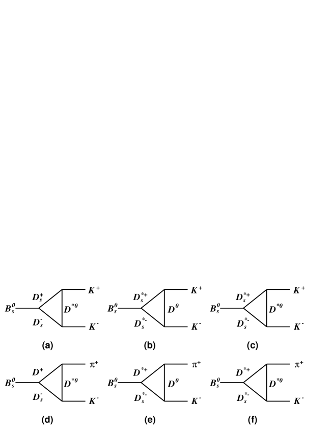
To evaluate the FSI effects, we calculate the absorptive part (see above arguments) of the one-particle-exchange triangle diagrams. Fig. 1 shows the diagrams of $B_{s}\rightarrow D_{s}^{(*)+}D_{s}^{(*)-}\rightarrow K^{+}K^{-}$ by exchanging $D^{0(*)}$. For calculating the absorptive part of the triangle, with the Cutkosky cutting rule Cheng:2004ru ; Shifman:1978bx , the related amplitudes are:

$$\mathcal{A}_{1}\Big{[}B_{s}(p)\rightarrow D_{s}^{+}(p_{1})D_{s}^{-}(p_{2})\rightarrow K^{+}(p_{3})K^{-}(p_{4})\Big{]}$$

$$={1\over 2}\int d\tilde{p}_{1}d\tilde{p}_{2}(2\pi)^{4}\delta(p-p_{1}-p_{2})\mathcal{A}\Big{[}B_{s}\rightarrow D_{s}^{+}(p_{1})D_{s}^{-}(p_{2})\Big{]}(-g_{KD_{s}D^{*}})\Big{[}-i(p_{1}+p_{3})_{\mu}\Big{]}(-g_{KD_{s}D^{*}})\Big{[}-i(p_{2}+p_{4})_{\nu}\Big{]}$$

$$\quad\times\Big{[}-g_{\mu\nu}+{q_{\mu}q_{\nu}\over m_{D^{0*}}^{2}}\Big{]}{i\over q^{2}-m_{D^{0*}}^{2}}\mathcal{F}^{2}(q^{2},m_{D^{0*}}^{2}),$$ (12a)

$$\mathcal{A}_{2}\Big{[}B_{s}(p)\rightarrow D_{s}^{*}(p_{1})D_{s}^{*}(p_{2})\rightarrow K^{+}(p_{3})K^{-}(p_{4})\Big{]}$$

$$={1\over 2}\int d\tilde{p}_{1}d\tilde{p}_{2}(2\pi)^{4}\delta(p-p_{1}-p_{2})\mathcal{A}\Big{[}B_{s}\rightarrow D_{s}^{+*}(p_{1})D_{s}^{-*}(p_{2})\Big{]}(-g_{KD_{s}^{*}D})\Big{[}-i(q+p_{3})_{\xi}\Big{]}(-g_{KD_{s}^{*}D})\Big{[}-i(q-p_{4})_{\sigma}\Big{]}$$

$$\quad\times\Big{[}-g_{\mu\xi}+{p_{1\mu}p_{1\xi}\over m_{D_{s}^{*}}^{2}}\Big{]}\Big{[}-g_{\nu\sigma}+{p_{2\nu}p_{2\sigma}\over m_{D_{s}^{*}}^{2}}\Big{]}{i\over q^{2}-m_{D^{0}}^{2}}\mathcal{F}^{2}(q^{2},m_{D^{0}}^{2}),$$ (12b)

$$\mathcal{A}_{3}\Big{[}B_{s}(p)\rightarrow D_{s}^{*+}(p_{1})D_{s}^{*-}(p_{2})\rightarrow K^{+}(p_{3})K^{-}(p_{4})\Big{]}$$

$$={1\over 2}\int d\tilde{p}_{1}d\tilde{p}_{2}(2\pi)^{4}\delta(p-p_{1}-p_{2})\mathcal{A}\Big{[}B_{s}\rightarrow D_{s}^{+*}(p_{1})D_{s}^{-*}(p_{2})\Big{]}(ig_{KD_{s}^{*}D^{*}})(-ip_{1\sigma})(-iq_{\alpha})\epsilon^{\sigma\omega\alpha\beta}(ig_{KD_{s}^{*}D^{*}})(-ip_{2\xi})(iq_{\kappa})$$

$$\quad\times\epsilon^{\xi\lambda\kappa\rho}\Big{[}-g_{\beta\rho}+{q_{\beta}q_{\rho}\over m_{D^{0*}}^{2}}\Big{]}\Big{[}-g_{\mu\omega}+{p_{1\mu}p_{1\omega}\over m_{D_{s}^{*}}^{2}}\Big{]}\Big{[}-g_{\nu\lambda}+{p_{2\nu}p_{2\lambda}\over m_{D_{s}^{*}}^{2}}\Big{]}{i\over q^{2}-m_{D^{0*}}^{2}}\mathcal{F}^{2}(q^{2},m_{D^{*0}}^{2}),$$ (12c)

instead, for the decay channel $$B_{s}\rightarrow D^{(*)+}D_{s}^{(*)-}\rightarrow\pi^{+}K^{-}$$, we have:

$$\mathcal{A}_{1}\Big{[}B_{s}(p)\rightarrow D^{+}(p_{1})D_{s}^{-}(p_{2})\rightarrow\pi^{+}(p_{3})K^{-}(p_{4})\Big{]}$$

$$={1\over 2}\int d\tilde{p}_{1}d\tilde{p}_{2}(2\pi)^{4}\delta(p-p_{1}-p_{2})\mathcal{A}\Big{[}B_{s}\rightarrow D^{+}(p_{1})D_{s}^{-}(p_{2})\Big{]}(-g_{\pi DD^{*}})\Big{[}-i(p_{1}+p_{3})_{\mu}\Big{]}(-g_{KD_{s}D^{*}})\Big{[}-i(p_{2}+p_{4})_{\nu}\Big{]}$$

$$\quad\times\Big{[}-g_{\mu\nu}+{q_{\mu}q_{\nu}\over m_{D^{0*}}^{2}}\Big{]}{i\over q^{2}-m_{D^{0*}}^{2}}\mathcal{F}^{2}(q^{2},m_{D^{0*}}^{2}),$$ (12d)

$$\mathcal{A}_{2}\Big{[}B_{s}(p)\rightarrow D^{*+}(p_{1})D_{s}^{*-}(p_{2})\rightarrow\pi^{+}(p_{3})K^{-}(p_{4})\Big{]}$$

$$={1\over 2}\int d\tilde{p}_{1}d\tilde{p}_{2}(2\pi)^{4}\delta(p-p_{1}-p_{2})\mathcal{A}\Big{[}B_{s}\rightarrow D^{+*}(p_{1})D_{s}^{-*}(p_{2})\Big{]}(-g_{\pi DD^{*}})\Big{[}-i(q+p_{3})_{\xi}\Big{]}(-g_{KD_{s}^{*}D})\Big{[}-i(q-p_{4})_{\sigma}\Big{]}$$

$$\quad\times\Big{[}-g_{\mu\xi}+{p_{1\mu}p_{1\xi}\over m_{D^{*}}^{2}}\Big{]}\Big{[}-g_{\nu\sigma}+{p_{2\nu p_{2\sigma}}\over m_{D_{s}^{*}}^{2}}\Big{]}{i\over q^{2}-m_{D^{0}}^{2}}\mathcal{F}^{2}(q^{2},m_{D^{0}}^{2}),$$ (12e)

$$\mathcal{A}_{3}\Big{[}B_{s}(p)\rightarrow D^{*+}(p_{1})D_{s}^{*-}(p_{2})\rightarrow\pi^{+}(p_{3})K^{-}(p_{4})\Big{]}$$

$$={1\over 2}\int d\tilde{p}_{1}d\tilde{p}_{2}(2\pi)^{4}\delta(p-p_{1}-p_{2})\mathcal{A}\Big{[}B_{s}\rightarrow D^{+*}(p_{1})D_{s}^{-*}(p_{2})\Big{]}(ig_{\pi D^{*}D^{*}})(-ip_{1\sigma})(-iq_{\alpha})\epsilon^{\sigma\omega\alpha\beta}(ig_{KD_{s}^{*}D^{*}})(-ip_{2\xi})(iq_{\kappa})$$

$$\quad\times\epsilon^{\xi\lambda\kappa\rho}\Big{[}-g_{\beta\rho}+{q_{\beta}q_{\rho}\over m_{D^{0*}}^{2}}\Big{]}\Big{[}-g_{\mu\omega}+{p_{1\mu}p_{1\omega}\over m_{D^{*}}^{2}}\Big{]}\Big{[}-g_{\nu\lambda}+{p_{2\nu}p_{2\lambda}\over m_{D_{s}^{*}}^{2}}\Big{]}{i\over q^{2}-m_{D^{0*}}^{2}}\mathcal{F}^{2}(q^{2},m_{D^{*0}}^{2}),$$ (12f)

where ${d\tilde{p}}=dp^{3}/((2\pi)^{3}2E)$, $q$ is the momentum of the exchanged $D^{0(*)}$ meson and a dipole form factor $\mathcal{F}(q^{2},m^{2})=(\Lambda^{2}-m^{2})^{2}/(\Lambda^{2}-q^{2})^{2}$ with $\Lambda=m+\beta\Lambda_{QCD}$ is introduced to compensate its off-shell effect Liu:2007qs .

$g$	value	$g$	value
$g_{D^{*}D\psi}$	$4.2\mathrm{GeV}^{-1}$ Liu:2007qs , ${\frac{7.7}{m_{D}}}$ GeV-1 Haglin:1999xs	$g_{DD\psi}$	7.9 Liu:2007qs , 8.0 Deandrea:2003pv
$g_{\pi DD^{*}}$	8.8 Haglin:1999xs	$g_{\pi D^{*}D^{*}}$	$8.9\,\mathrm{GeV}^{-1}$ Liu:2007qs , 9.1 $\mathrm{GeV}^{-1}$ Oh:2000qr

Table 2: The values of the coupling constants involved in our work.

III Numerical result

With the amplitudes given in Eq. (12), we can easily calculate the decay width of the sequential processes $B_{s}\rightarrow D_{s}^{(*)}D_{s}^{(*)}\rightarrow K^{+}K^{-}$. We take the relevant parameters from PDG PDG10 as: $m_{B_{s}}=5.366\,\mathrm{GeV}$, $m_{D_{s}}=1.968\,\mathrm{GeV}$, $m_{D^{*}_{s}}=2.112\,\mathrm{GeV}$, $m_{D^{0}}=1.864\,\mathrm{GeV}$, $m_{D^{0*}}=2.007\,\mathrm{GeV}$, $m_{D^{\pm}}=1.869\,\mathrm{GeV}$, $m_{D^{*\pm}}=2.01\,\mathrm{GeV}$; and the value of the weak decay constants, such as $f_{\pi}\;f_{K}\;f_{D}\;f_{D_{s}}$ can be found in Ref. Azizi:2008ty ; $a_{1}=1.14$ is set in our numerical computations Ablikim:2002ep . The total amplitudes are

$$\Big{|}\mathcal{A}(B_{s}\rightarrow K^{+}K^{-})\Big{|} = \Big{|}\mathcal{A}^{\mathrm{direct}}(B_{s}\rightarrow K^{+}K^{-})+\mathcal{A}_{1}(B_{s}\rightarrow D_{s}^{+}D_{s}^{-}\rightarrow K^{+}K^{-})+\mathcal{A}_{2}(B_{s}\rightarrow D_{s}^{*+}D_{s}^{*-}\rightarrow K^{+}K^{-})$$ (13)

$$+\mathcal{A}_{3}(B_{s}\rightarrow D_{s}^{*+}D_{s}^{*-}\rightarrow K^{+}K^{-})\Big{|}=(4.1\pm 0.8)\times 10^{-8},$$

$$\Big{|}\mathcal{A}(B_{s}\rightarrow\pi^{+}K^{-})\Big{|} = \Big{|}\mathcal{A}^{\mathrm{direct}}(B_{s}\rightarrow\pi^{+}K^{-})+\mathcal{A}_{1}(B_{s}\rightarrow D^{+}D_{s}^{-}\rightarrow\pi^{+}K^{-})+\mathcal{A}_{2}(B_{s}\rightarrow D^{*+}D_{s}^{*-}\rightarrow\pi^{+}K^{-})$$ (14)

$$+\mathcal{A}_{3}(B_{s}\rightarrow D^{*+}D_{s}^{*-}\rightarrow\pi^{+}K^{-})\Big{|}=30.4^{+0.2}_{-0.1}\times 10^{-9},$$

where $A^{\mathrm{direct}}(B_{s}\rightarrow K^{+}K^{-})$ is the penguin contribution Cheng . So, the branching ratios are:

$$\mathcal{B}(B_{s}\rightarrow K^{+}K^{-}) = {\Gamma_{B_{s}\rightarrow K^{+}K^{-}}\over\Gamma_{\mathrm{tot}}}={1\over 32\pi^{2}\Gamma_{\mathrm{tot}}}{\Big{|}p_{K}\Big{|}\over m_{B_{s}}^{2}}\Big{|}\mathcal{A}_{\mathrm{tot}}(B_{s}\rightarrow KK)\Big{|}^{2}d\Omega=13.6^{+6.3}_{-5.1}\times 10^{-6},$$

$$\mathcal{B}(B_{s}\rightarrow\pi^{+}K^{-}) = {\Gamma_{B_{s}\rightarrow\pi K}\over\Gamma_{\mathrm{tot}}}={1\over 32\pi^{2}\Gamma_{\mathrm{tot}}}{\Big{|}p_{K}\Big{|}\over m_{B_{s}}^{2}}\Big{|}\mathcal{A}_{\mathrm{tot}}(B_{s}\rightarrow K\pi)\Big{|}^{2}d\Omega=7.8^{+0.1}_{-0.1}\times 10^{-6},$$

where the errors are systematical, originating from the uncertainty of the coupling constants.

Table 3: Various approaches predictions on $\mathcal{B}(B_{s}\to K^{+}K^{-})$ (in units of $10^{-6}$).

and the ratio $\mathcal{R}=\mathcal{B}(B_{s}\rightarrow\pi^{+}K^{-})/\mathcal{B}(B_{s}\rightarrow K^{+}K^{-})$ QCDF Cheng pQCD (LO) Ali:2007ff pQCD (NLO) Liu:2008rz SCET Williamson:2006hb FSI FSI+pQCD (NLO) Experiment Abulencia:2006psa ; Aaltonen:2008hg $\mathcal{B}$ $25.2^{+12.7+12.5}_{-7.2-9.1}$ $13.6^{+8.6}_{-5.2}$ $15.6^{+5.1}_{-3.9}$ $18.2\pm 6.7\pm 1.1\pm 0.5$ ${13.6^{+6.3}_{-5.1}}$ ${29.2^{+8.1}_{-6.5}}$ $33\pm 9$ $\mathcal{R}$ 0.194 0.360 0.314 0.269 0.360 0.167 0.148

In Table 3 we list the theoretical predictions on $\mathcal{B}(B_{s}\to K^{+}K^{-})$ in various approaches. It is noted that most of the predicted cental values are lower than the newly measured value Cheng ; Ali:2007ff ; Liu:2008rz ; Williamson:2006hb as long as the contribution from FSI is not included. We add the contributions from FSI to that calculated in pQCD (NLO), then one can find that the resultant central value is consistent with data Beringer:1900zz : $\mathcal{B}(B_{s}\rightarrow K^{+}K^{-})=(3.3\pm 0.9)\times 10^{-5}$ within $1\sigma$.

The deviations of our theoretical prediction from the data might come from the loophole in our calculation. As indicated above we only consider the absorptive part of the hadronic triangle. Indeed the dispersive part may also make substantial contributions Liu:2006dq . As suggested in literature, the dispersive contribution should be smaller than the absorptive one (it is consistent with the general principle of the quantum field theory), or at most has the same magnitude as that of the absorptive part. If the contribution of the dispersive part is indeed of the same order as the absorptive part, then taking it into account, we may have a result, which is even closer to the data.

In general, even though we cannot precisely re-produce the experimental data, we can confirm ourselves that the FSI is important and non-negligible for understanding the $\mathcal{B}(B_{s}\rightarrow K^{+}K^{-})>\mathcal{B}(B_{s}\rightarrow\pi^{+}K^{-})$ “conflict”.

IV Conclusion and Discussion

As expected, the LHCb is extensively aiming on study of the B-physics, especially to look for some ”anomalies” in experiments, which need high statistics and precise measurements. For $B_{s}$’s charmless non-leptonic two-body decay, the early MC studies show that, nearly 37K $B_{s}\rightarrow K^{+}K^{-}$ signals will be seen at $2\ fb^{-1}$ integrated luminosity Rademacker:2007zza . On the other hand, $314\pm 27$ $B_{s}\rightarrow\pi^{+}K^{-}$ signals were observed based on the 2010 data with its integrated luminosity $0.35fb^{-1}$ Aaij:2012qe . We believe that the statistics of the $B_{s}$ decay into $K^{+}K^{-}$ and $\pi^{+}K^{-}$ is sufficient to draw a definite decision about their branching ratios. The latest result reported by the LHCb collaboration shows that the branching ratios have been measured as :2012as :

$${\mathcal{B}(H_{b}\rightarrow F)\over\mathcal{B}(H_{b}^{\prime}\rightarrow F^{\prime})}={f_{H^{\prime}_{b}}\over f_{H_{b}}}{N(H_{b}\rightarrow F)\over N(H^{\prime}_{b}\rightarrow F^{\prime})}{\epsilon_{\mathrm{rec}}(H^{\prime}_{b}\rightarrow F^{\prime})\over\epsilon_{\mathrm{rec}}(H_{b}\rightarrow F)}{\epsilon_{\mathrm{PID}}(F^{\prime})\over\epsilon_{\mathrm{PID}}(F)},$$ (16)

where the $f_{H^{(^{\prime})}_{b}}$ is the possibility of $b$ quark hadronizing into hadron $H$, $N$ is the observed number of signals for certain decay modes, $\epsilon_{\mathrm{rec}}$ is the efficiency of the reconstruction excluding the particle identification (PID) cuts and $\epsilon_{\mathrm{PID}}$ is just the efficiency of PID cuts.

It is noted that in Table III, the experimental data are taken from Refs. Abulencia:2006psa ; Aaltonen:2008hg , but the 2012 data of PDG indicate that the branching ratio of $B_{s}\to K^{+}K^{-}$ is $(2.64\pm 0.28)\times 10^{-5}$ Beringer:1900zz , which is smaller than the data in Ref. Abulencia:2006psa ; Aaltonen:2008hg . Moreover, the LHCb collaboration reports that with the $0.37fb^{-1}$ 2011 data, the branching ratios of $B_{s}\rightarrow K^{+}K^{-}$ and $B_{s}\rightarrow\pi^{+}K^{-}$ are experimentally determined as:

$$\begin{aligned} \mathcal{B}(B_{s}\rightarrow K^{+}K^{-})&=(23.0\pm 0.7\pm 2.3)\times 10^{-6},\\ \mathcal{B}(B_{s}\rightarrow\pi^{+}K^{-})&=(5.4\pm 0.4\pm 0.6)\times 10^{-6},\end{aligned}$$ (17)

where the former uncertainties are statistical and the later one is systematical, which include the uncertainties of PID calibration, final state radiation with soft gamma, signal shape used for fitting, and the impact of the background: the additional three-body background, the combinatorial background and the cross-feed background. Since $B_{s}\rightarrow K^{+}K^{-}$ and $B_{s}\rightarrow D^{(*)+}_{s}\bar{D}^{(*)-}_{s}\rightarrow K^{+}K^{-}$ have the same final states, it means we cannot single out the contributions of FSI by simply measuring the cross section in experiments. Even though our theoretical prediction on $\mathcal{B}(B_{s}\to K^{+}K^{-})$ presented in Table 3 is slightly above the value of the LHCb measurements, it is still consistent with the data within the experimental error tolerance. Therefore we are expecting more precise measurements in the future.

Cheng and Chua suggested that the decay $B_{s}\to K^{+}K^{-}$ is dominated by the penguin diagram, which does not suffer from large CKM suppression Cheng . In that scenario the “conflict” $\mathcal{B}(B_{s}\to K^{+}K^{-})>\mathcal{B}(B_{s}\to\pi^{+}K^{-})$ could be partly explained. In our work, we show that the FSI definitely makes an important contribution because $B_{s}\to D_{s}^{(*)}\bar{D}_{s}^{(*)}$ are dominant decay modes of $B_{s}$ as confirmed by the data and the scattering $D_{s}^{(*)+}D_{s}^{(*)-}\to K^{+}K^{-}$ is allowed by all the symmetry requirements. Therefore, we might consider that the penguin contribution and the FSI effects are in parallel to contribute to the decay $B_{s}\to K^{+}K^{-}$. Actually, there are several phenomenological parameters in the model for evaluating the FSI effects, which were obtained by fitting the earlier data of heavy flavor processes. One thing can be sure that the FSI should exist and contribute to the process $B_{s}\to K^{+}K^{-}$, but how significant it would be is determined by both requirement of experimental measurements and theoretical estimate. If the data on $\mathcal{B}(B_{s}\to K^{+}K^{-})$ are indeed going down, the FSI effects for $B_{s}\to K^{+}K^{-}$ would be less significant, by that situation, one can further restrict the involved phenomenological parameters at this energy region. On other aspect, the errors of the measurements are still too large to make a definite conclusion yet, so we are expecting more precise measurements not only from LHCb, but also the future super-B factory.

Definitely the FSI effects also play roles in other similar decay channels, such as $B^{\pm}\rightarrow K^{\pm}\omega$. Therefore careful studies on such modes with the same theoretical framework would be helpful for more accurately evaluating the FSI effects. The PDG indicates that, $\mathcal{B}(B^{\pm}\rightarrow K^{\pm}\omega)/\mathcal{B}(B^{\pm}\rightarrow\pi^{\pm}\omega)=(6.7\times 10^{-6})/(6.9\times 10^{-6})$, so one would expect that $\mathcal{B}(B\rightarrow K\omega)$ is also enhanced by the FSI. Moreover, a measurement on the polarization of $\omega$ might be helpful to gain more information about the role of the FSI mechanism, and it will be studied in our coming work.

From the experimental aspect, as the FSI is a scattering fully governed by the strong interaction, its proper time is too short to be measured in the LHCb detector. Although the LHCb can well reconstruct the events $B_{s}\rightarrow K^{+}(\pi^{+})K^{-}$ and identify the $\pi^{+}K^{-}$ purely with the PID cuts Karbach:2012sw , it is impossible to distinguish between the direct decays $B_{s}\to K^{+}(\pi^{+})K^{-}$ and the sequential ones. Considering the good ability of LHCb for tracking charged particles, we believe that, $B^{\pm}\rightarrow K(\pi)^{\pm}\omega$ is another good channel to study FSI. The decay rates of $\mathcal{B}(B\rightarrow\bar{D}^{0}D^{(*)+})$ have been well measured as $\sim 1.8\pm 0.2\times 10^{-2}$, and we can make Mont-Carlo simulations on the re-scattering of $\bar{D}^{0}D_{s}^{(*)+}$ into $K(\pi)^{+}\omega$ to complete the theoretical scenario. The abnormal ratio of the two channels $\mathcal{B}(B^{\pm}\rightarrow K^{\pm}\omega)/\mathcal{B}(B^{\pm}\rightarrow\pi^{\pm}\omega)=(6.7\times 10^{-6})/(6.9\times 10^{-6})$ Beringer:1900zz can also be explained as the FSI contribution as well. With $B^{\pm}\rightarrow DK(\pi)^{\pm}$ measurement Aaij:2012kz and considering the efficiency, about 0.8K $B^{+}\rightarrow K(\pi)^{+}\omega$ can been seen in the 2011 database and it implies that the FSI contribution to the polarization of the vector meson $\omega$ might be distinguished from that of the direct decay. Comparing more accurate data with our theoretical calculation, one can expect to gain more knowledge on the FSI effects, for example how to determine the parameters in the dipole form factor etc.

One object can be recommended for pining down the role of the FSI effects. As well known that the direct CP violation is proportional to $\sin(\alpha_{1}-\alpha_{2})\cdot\sin(\phi_{1}-\phi_{2})$, where the subscripts 1 and 2 refer to two different routes and $\alpha$, $\phi$ are the weak and strong phases respectively. Therefore, if a direct CP violation exists in $B_{s}$ decays, there must at least be two different routes to the final states which possess different weak and strong phases. In fact, the penguin and tree diagrams have different strong and weak phases. The weak phase of the tree diagram is coming from $V_{ub}V^{*}_{us}$ and does not posses a strong phase. Instead, the weak phase of the penguin is from $V_{cb}V^{*}_{cs}$ and the strong phase is due to existence of the absorptive part of the loop. In our scenario the sequential processes $B_{s}(\bar{B}_{s})\to D_{s}^{(*)}\bar{D}_{s}^{(*)}\to K^{+}K^{-}$ which have the same weak phase $V_{cb}V^{*}_{cs}$, but different strong phase from the penguin. Because of the extra contribution, the amplitude would become

$$M=M^{tree}e^{i\alpha_{1}}+M^{penguin}e^{i(\alpha_{2}+\phi_{1})}+M^{seq}e^{i(\alpha_{2}+\phi_{2})},$$

where the last term is the FSI contribution.

Thus the interference between the tree diagram with a sum of the penguin and sequential processes would be different from the situation where the tree diagram only interferes with the penguin. Therefore by measuring the CP violation of $\mathcal{B}(B_{s}\to K^{+}K^{-})-\mathcal{B}(\bar{B}_{s}\to K^{+}K^{-})$, one can distinguish between the penguin contributions and the FSI effects. But since the experimental errors and theoretical uncertainties are not well controlled so far, we cannot make a more definite prediction on the CP violation yet, we would wait for more precise data to be available and then continue our theoretical computations.

Moreover, according to the above arguments, there does not exist a tree diagram for $B_{s}\to K^{0}\bar{K}^{0}$. Consequently, the direct transition $B_{s}\to K^{0}\bar{K}^{0}$ is uniquely determined by the penguin diagram and FSI effects. Because the tree contribution to $B_{s}\to K^{+}K^{-}$ is very small, the rate of $B_{s}\to K^{0}\bar{K}^{0}$ must be close to that of $B_{s}\to K^{+}K^{-}$. However the interference between penguin (neglecting the Cabibbo-suppressed penguin diagrams where $t$-quark and $u$-quark are intermediate agents) and FSI does not lead to a direct CP violation at all, because they have the same weak phase. This can be confirmed by future experiments.

References

• (1) A. Abulencia et al. [CDF Collaboration], Phys. Rev. Lett.  98, 061802 (2007) [hep-ex/0610045].
• (2) R. Louvot et al. [Belle Collaboration], Phys. Rev. Lett.  102, 021801 (2009) [arXiv:0809.2526 [hep-ex]].
• (3) K. Nakamura et al. [Particle Data Group], J. Phys. G 37, 075021 (2010).
• (4) A. Abulencia et al. [CDF Collaboration], Phys. Rev. Lett.  97, 211802 (2006) [hep-ex/0607021].
• (5) T. Aaltonen et al. [CDF Collaboration], Phys. Rev. Lett.  103, 031801 (2009) [arXiv:0812.4271 [hep-ex]].
• (6) S. Descotes-Genon, J. Matias and J. Virto, Phys. Rev. Lett.  97, 061801 (2006) [hep-ph/0603239].
• (7) H. -Y. Cheng and C. -K. Chua, Phys. Rev. D 80, 114026 (2009) [arXiv:0910.5237 [hep-ph]].
• (8) A. Ali, G. Kramer, Y. Li, C. -D. Lu, Y. -L. Shen, W. Wang and Y. -M. Wang, Phys. Rev. D 76, 074018 (2007) [hep-ph/0703162 [HEP-PH]].
• (9) J. Liu, R. Zhou and Z. -J. Xiao, arXiv:0812.2312 [hep-ph].
• (10) A. R. Williamson and J. Zupan, Phys. Rev. D 74, 014003 (2006) [Erratum-ibid. D 74, 03901 (2006)] [hep-ph/0601214].
• (11) Y. -S. Dai, D. -S. Du, X. -Q. Li, Z. -T. Wei and B. -S. Zou, Phys. Rev. D 60, 014014 (1999) [hep-ph/9903204].
• (12) S. G. Matinyan and B. Muller, Phys. Rev. C 58, 2994 (1998).
• (13) M. Ablikim, D. -S. Du and M. -Z. Yang, Phys. Lett. B 536, 34 (2002).
• (14) K. L. Haglin, Phys. Rev. C 61 (2000) 031902.
• (15) Z. -W. Lin and C. M. Ko, Phys. Rev. C 62, 034903 (2000).
• (16) G. Buchalla, A. J. Buras and M. E. Lautenbacher, Rev. Mod. Phys.  68, 1125 (1996).
• (17) H. -Y. Cheng, C. -K. Chua and C. -W. Hwang, Phys. Rev. D 69, 074025 (2004).
• (18) H. -Y. Cheng, Z. Phys. C 32, 237 (1986).
• (19) X. -Q. Li, T. Huang and Z. -C. Zhang, Z. Phys. C 42, 99 (1989).
• (20) M. A. Shifman, A. I. Vainshtein and V. I. Zakharov, Nucl. Phys. B 147, 385 (1979).
• (21) H. -Y. Cheng, C. -K. Chua and A. Soni, Phys. Rev. D 71, 014030 (2005) [hep-ph/0409317].
• (22) X. Liu and X. -Q. Li, Phys. Rev. D 77, 096010 (2008) [arXiv:0707.0919 [hep-ph]].
• (23) R. Casalbuoni, A. Deandrea, N. Di Bartolomeo, R. Gatto, F. Feruglio andG. Nardulli, Phys. Rept. 281, 145 (1997)[hep-ph/9605342];A. Deandrea, N. Di Bartolomeo, R. Gatto, G. Nardulli and A. D. Polosa, Phys. Rev. D 58, 034004 (1998)[hep-ph/9802308].
• (24) A. Deandrea, G. Nardulli and A. D. Polosa, Phys. Rev. D 68, 034002 (2003)[hep-ph/0302273].
• (25) K. L. Haglin and C. Gale, Phys. Rev. C 63, 065201 (2001).
• (26) Y. -S. Oh, T. Song and S. H. Lee, Phys. Rev. C 63, 034901 (2001) [nucl-th/0010064].
• (27) K. Azizi, R. Khosravi and F. Falahati, Int. J. Mod. Phys. A 24, 5845 (2009).
• (28) X. Liu, X. -Q. Zeng and X. -Q. Li, Phys. Rev. D 74, 074003 (2006) [hep-ph/0606191].
• (29) J. Rademacker [LHCb Collaboration], Acta Phys. Polon. B 38, 955 (2007).
• (30) R. Aaij et al. [LHCb Collaboration], Phys. Rev. Lett.  108, 201601 (2012).
• (31) RAaij et al. [LHCb Collaboration], arXiv:1206.2794 [hep-ex].
• (32) J. Beringer et al. [Particle Data Group Collaboration], Phys. Rev. D 86, 010001 (2012).
• (33) T. M. Karbach [LHCb Collaboration], arXiv:1205.6579 [hep-ex].
• (34) R. Aaij et al. [LHCb Collaboration], Phys. Lett. B 712, 203 (2012) [arXiv:1203.3662 [hep-ex]].