Effects of Refraction and Reflection on Coherence Properties of Light

Abstract

Partially coherent light beams are encountered both in classical and in quantum optics. Their coherence properties generally depend on the correlation properties of their sources. In this paper, we propose a technique for controlling the coherence properties of optical beams in laboratory environment. The technique is based on the fact that coherence properties of partially coherent electromagnetic beams can be changed on refraction and on reflection, and that the changes can be controlled by varying the angle of incidence.

Introduction

Coherence properties of light play important roles in many experiments both in classical and quantum optics. These properties are generally determined by the correlation properties of the source, which generates the light. Change of coherence properties of light due to propagation (BW , Ch. 10) and scattering (EW , Ch. 6) have been studied in great detail. However, such changes cannot easily be controlled in a laboratory environment. We propose a method of controlling them in optical experiments. We show that coherence properties of partially coherent beams can be both improved and degraded by means of reflection or refraction at a surface separating two media of different dielectric properties. We also show that such changes can be controlled by varying the angle of incidence.

Properties of refracted and reflected light are usually studied by employing the classic Fresnel formulas. An account of the theory leading to them can be found, for example, in Ref. Jackson , chapter 7. The treatment is based on the assumption that the incident, the refracted and the transmitted electromagnetic fields are monochromatic plane waves. The Fresnel formulas, therefore, do not apply to partially coherent beams, and they cannot provide any information as to whether coherence properties of light can change on refraction or on reflection. However, one can use them to formulate a general theory of refraction and reflection for partially coherent beams. Application of the generalized formulation shows that coherence properties of a partially coherent beam change, in general, on refraction and on reflection.

Coherence theory of stochastic electromagnetic beams

In the optical and in the higher frequency ranges of the electromagnetic spectrum, the concept of monochromaticity is an idealization, which is not encountered in practice. All optical fields exhibit some random fluctuations. If these fluctuations are assumed to be statistically stationary, the field can be represented, at each frequency $\omega$, by an ensemble $\left\{\mathbf{E}(\mathbf{r},\omega)\right\}$ of monochromatic vector fields (see, for example, EW , Sec. 4.1). When the field is beam-like, one can neglect the field components along the propagation direction. Hence, each member of the ensemble of electric field can be represented in terms of two mutually orthogonal components, each of which is perpendicular to the direction of propagation. We label them by the symbols v and h. Each member of the ensemble of the electric field vectors can be represented as a column matrix, i.e., in the form

$$\mathbf{E}(\mathbf{r},\omega)=\begin{pmatrix}E_{\text{v}}(\mathbf{r},\omega)\\ E_{\text{h}}(\mathbf{r},\omega)\end{pmatrix}=\begin{pmatrix}E_{\text{v}}(\mathbf{r},\omega)&\quad E_{\text{h}}(\mathbf{r},\omega)\end{pmatrix}^{T},$$ (1)

where the superscript $T$ denotes the transpose of the matrix. The second-order correlation properties of such a field Note-quant-coh-order are characterized by a $2\times 2$ correlation matrix $\overleftrightarrow{W}(\mathbf{r}_{1},\mathbf{r}_{2};\omega)$, the so-called cross-spectral density matrix (CSDM), which is defined, at a pair of points specified by position vectors $\mathbf{r}_{1}$ and $\mathbf{r}_{2}$, by the formula (EW , Ch. 9)

$$\overleftrightarrow{W}(\mathbf{r}_{1},\mathbf{r}_{2};\omega)=\left\langle\mathbf{E}^{\ast}(\mathbf{r}_{1};\omega)\cdot\mathbf{E}^{T}(\mathbf{r}_{2};\omega)\right\rangle.$$ (2)

Here the asterisk denotes the complex conjugate, the dot denotes matrix multiplication, and the angular brackets denote the ensemble average. Clearly a typical element of the CSDM is $W_{lm}(\mathbf{r}_{1},\mathbf{r}_{2};\omega)=\langle E_{\text{l}}^{\ast}(\mathbf{r}_{1};\omega)E_{\text{m}}(\mathbf{r}_{2};\omega)\rangle$; $l$=h,v; $m$=h,v.

Coherence properties of an optical beam characterize its ability to interfere. The simplest types of coherence properties are characterized by the visibility of fringes produced in an Young’s interference experiment. Suppose that a light beam is incident on an opaque screen containing two pinholes located at points $\mathbf{r}_{1}$ and $\mathbf{r}_{2}$. The visibility of the interference fringes produced by the frequency component $\omega$ at another screen placed sufficiently far behind the pinholes, is given by the modulus $|\eta(\mathbf{r}_{1},\mathbf{r}_{2};\omega)|$ of the spectral degree of coherence, i.e., of the spatial degree of coherence at frequency $\omega$, defined by the formula (EW , Ch. 9)

$$\eta(\mathbf{r}_{1},\mathbf{r}_{2};\omega)\equiv\frac{\text{Tr}~{}\overleftrightarrow{W}(\mathbf{r}_{1},\mathbf{r}_{2};\omega)}{\sqrt{\text{Tr}~{}\overleftrightarrow{W}(\mathbf{r}_{1},\mathbf{r}_{1};\omega)}\sqrt{\text{Tr}~{}\overleftrightarrow{W}(\mathbf{r}_{2},\mathbf{r}_{2};\omega)}},$$ (3)

where Tr $\overleftrightarrow{W}$ denotes the trace of the matrix $\overleftrightarrow{W}$. It can readily be shown that $0\leq|\eta(\mathbf{r}_{1},\mathbf{r}_{2};\omega)|\leq 1$. When $|\eta(\mathbf{r}_{1},\mathbf{r}_{2};\omega)|=1$, i.e., when the fringe-visibility is maximum, the beam is said to be spatially completely coherent at the pair of points $(\mathbf{r}_{1},\mathbf{r}_{2})$. In the other extreme case when $\eta(\mathbf{r}_{1},\mathbf{r}_{2};\omega)=0$, the beam is said to be spatially incoherent at the two points. In any intermediate case ($0<|\eta(\mathbf{r}_{1},\mathbf{r}_{2};\omega)|<1$), the beam is said to be partially coherent at the two points, at frequency $\omega$.

Another definition of the degree of coherence of electromagnetic beams have been proposed (for some discussions relating to this topic see STF1 ; W-comment ; STF1-re-comment ). For our purpose, it is immaterial which of the two definitions is used. In this paper, we use the definition in terms of fringe visibility, because it is often employed in the analysis of experimental results (see, for example, Laura-coh-synth ).

Fresnel formulas for reflection and refraction of monochromatic plane waves

Let us first consider refraction and reflection of a monochromatic plane wave at a planar interface that separates two homogeneous media. Suppose that dielectric properties of the two media are characterized by permittivities and permeabilities $\epsilon$, $\mu$, and $\epsilon^{\prime}$, $\mu^{\prime}$. Their refractive indices are given by $n=\sqrt{\epsilon\mu/\epsilon_{0}\mu_{0}}$, and $n^{\prime}=\sqrt{\epsilon^{\prime}\mu^{\prime}/\epsilon_{0}\mu_{0}}$, respectively (see, for example, Jackson , p. 303). Here $\epsilon_{0}\approx 8.854\times 10^{-12}$ F$/$m is the vacuum permittivity, and $\mu_{0}\approx 1.257\times 10^{-6}$ H$/$m is the vacuum permeability.

Suppose that a monochromatic plane wave is incident on the interface at an angle of incidence $\theta_{\mathbb{i}}$ (see Fig. 1). The electric field vector of the incident wave can be expressed in the form $\mathbf{E}^{(\mathbb{i})}(\mathbf{r},t)=\mathbf{E}_{0}^{(\mathbb{i})}\exp\left[i(\mathbf{k}^{(\mathbb{i})}\cdot\mathbf{r}-\omega t)\right],$ where $\mathbf{k}^{(\mathbb{i})}$ is the wave vector. Similarly, the transmitted and the reflected electric field vectors may be represented by the expressions $\mathbf{E}^{(\mathbb{t})}(\mathbf{r},t)=\mathbf{E}_{0}^{(\mathbb{t})}\exp\left[i(\mathbf{k}^{(\mathbb{t})}\cdot\mathbf{r}-\omega t)\right],$ and $\mathbf{E}^{(\mathbb{r})}(\mathbf{r},t)=\mathbf{E}_{0}^{(\mathbb{r})}\exp\left[i(\mathbf{k}^{(\mathbb{r})}\cdot\mathbf{r}-\omega t)\right],$ respectively. The moduli of the wave vectors are given by the formulas $\left|\mathbf{k}^{(\mathbb{t})}\right|=\omega\sqrt{\epsilon^{\prime}\mu^{\prime}}$, and $\left|\mathbf{k}^{(\mathbb{i})}\right|=\left|\mathbf{k}^{(\mathbb{r})}\right|=\omega\sqrt{\epsilon\mu}$ [see, for example, Jackson , Eq. (7.33)]. The plane formed by the wave vector $\mathbf{k}^{(\mathbb{i})}$ and the normal $\mathbf{n}$ to the interface defines the plane of incidence. The refracted and the reflected wave vectors also lie in this plane.

Because electromagnetic waves are transverse, there is no component of the electric field vector in the direction of propagation of the incident plane wave. Hence, $\mathbf{E}^{(\mathbb{i})}$ can be expressed in terms of two mutually orthogonal components $\mathbf{E}_{\text{v}}^{(\mathbb{i})}$ and $\mathbf{E}_{\text{h}}^{(\mathbb{i})}$, i.e., $\mathbf{E}^{(\mathbb{i})}(\mathbf{r},t)=\mathbf{E}_{\text{v}}^{(\mathbb{i})}(\mathbf{r},t)+\mathbf{E}_{\text{h}}^{(\mathbb{i})}(\mathbf{r},t)=\left(\mathbf{E}_{0\text{v}}^{(\mathbb{i})}+\mathbf{E}_{0\text{h}}^{(\mathbb{i})}\right)\exp\left[i(\mathbf{k}^{(\mathbb{i})}\cdot\mathbf{r}-\omega t)\right]$. We choose $\mathbf{E}_{\text{v}}^{(\mathbb{i})}$ and $\mathbf{E}_{\text{h}}^{(\mathbb{i})}$ to be perpendicular and parallel, respectively, to the plane of incidence (see Fig. 1). Similarly the transmitted and the reflected electric fields can be uniquely decomposed in the v and the h directions, i.e., one has $\mathbf{E}^{(\mathbb{t})}(\mathbf{r},t)=\left(\mathbf{E}_{0\text{v}}^{(\mathbb{t})}+\mathbf{E}_{0\text{h}}^{(\mathbb{t})}\right)\exp\left[i(\mathbf{k}^{(\mathbb{t})}\cdot\mathbf{r}-\omega t)\right]$, and $\mathbf{E}^{(\mathbb{r})}(\mathbf{r},t)=\left(\mathbf{E}_{0\text{v}}^{(\mathbb{r})}+\mathbf{E}_{0\text{h}}^{(\mathbb{r})}\right)\exp\left[i(\mathbf{k}^{(\mathbb{r})}\cdot\mathbf{r}-\omega t)\right],$ respectively.

At the interface, the components of the transmitted and of the reflected fields are related to the components of the incident field by the well known Fresnel formulas, which can be expressed in the matrix form as

$$\mathbf{E}_{0}^{(\mathbb{t})}=\overleftrightarrow{\text{T}}\cdot\mathbf{E}_{0}^{(\mathbb{i})},\qquad\mathbf{E}_{0}^{(\mathbb{r})}=\overleftrightarrow{\text{R}}\cdot\mathbf{E}_{0}^{(\mathbb{i})}.$$ (4)

Here $\overleftrightarrow{\text{T}}=\bigl{(}\begin{smallmatrix}T_{\text{v}}&0\\ 0&T_{\text{h}}\end{smallmatrix}\bigr{)}$ and $\overleftrightarrow{\text{R}}=\bigl{(}\begin{smallmatrix}R_{\text{v}}&0\\ 0&R_{\text{h}}\end{smallmatrix}\bigr{)}$ are two diagonal matrices, whose elements are given by [see, for example, Jackson , Eqs. (7.39), and (7.41)]

$$T_{\text{v}} =\frac{2n\cos\theta_{\mathbb{i}}}{n\cos\theta_{\mathbb{i}}+\frac{\mu}{\mu^{\prime}}\sqrt{n^{\prime 2}-n^{2}\sin^{2}\theta_{\mathbb{i}}}},\qquad T_{\text{h}}=\frac{2nn^{\prime}\cos\theta_{\mathbb{i}}}{\frac{\mu}{\mu^{\prime}}n^{\prime 2}\cos\theta_{\mathbb{i}}+n\sqrt{n^{\prime 2}-n^{2}\sin^{2}\theta_{\mathbb{i}}}},$$ (5a)

$$R_{\text{v}} =\frac{n\cos\theta_{\mathbb{i}}-\frac{\mu}{\mu^{\prime}}\sqrt{n^{\prime 2}-n^{2}\sin^{2}\theta_{\mathbb{i}}}}{n\cos\theta_{\mathbb{i}}+\frac{\mu}{\mu^{\prime}}\sqrt{n^{\prime 2}-n^{2}\sin^{2}\theta_{\mathbb{i}}}},\qquad R_{\text{h}}=\frac{\frac{\mu}{\mu^{\prime}}n^{\prime 2}\cos\theta_{\mathbb{i}}-n\sqrt{n^{\prime 2}-n^{2}\sin^{2}\theta_{\mathbb{i}}}}{\frac{\mu}{\mu^{\prime}}n^{\prime 2}\cos\theta_{\mathbb{i}}+n\sqrt{n^{\prime 2}-n^{2}\sin^{2}\theta_{\mathbb{i}}}},$$ (5b)

$\theta_{\mathbb{i}}$ being the angle of incidence.

Theory of refraction and reflection with partially coherent beams

While dealing with partially coherent beams, one does not have the simplicity associated with monochromatic plane waves. One must then consider the effects of random fluctuations that are present in the electric field. Moreover, since partially coherent beams are not plane waves, one needs to employ the angular spectrum representation to study their properties (for a basic description of angular spectrum representation see, for example, MW , Sec. 3.2). According to the theory relating to such a representation, a partially coherent beam may be represented as superposition of ensembles of homogeneous and of evanescent plane waves. However, if one does not consider total internal reflection, the contribution from evanescent waves can usually be neglected Note-tot-int-refl . On refraction (reflection) of a partially coherent incident beam, the plane wave components present in it are individually refracted (reflected). Each of the plane wave components has a different direction of propagation, and, therefore, their angles of incidence are, in general, different from each other. Hence, the Fresnel coefficients have different values for each plane wave component. After refraction and reflection the plane waves will recombine to generate the transmitted and the reflected partially coherent beams. Because each plane wave undergo transformation characterized by different Fresnel coefficients, the beams generated by their recombination after refraction and reflection have coherence properties which are, in general, different from those of the incident beam.

The phenomenon can readily be described mathematically. It is useful to introduce separate coordinate systems for the incident, for the transmitted, and for the reflected beams. Let us denote them by $(x_{\text{v}}^{(\mathbb{i})},x_{\text{h}}^{(\mathbb{i})},x_{\text{p}}^{(\mathbb{i})})$, $(x_{\text{v}}^{(\mathbb{t})},x_{\text{h}}^{(\mathbb{t})},x_{\text{p}}^{(\mathbb{t})})$, and $(x_{\text{v}}^{(\mathbb{r})},x_{\text{h}}^{(\mathbb{r})},x_{\text{p}}^{(\mathbb{r})})$ respectively. We define each of them as follows: We choose the positive direction of the $x_{\text{p}}^{(l)}$ –axis ($l=\mathbb{i},\mathbb{t},\mathbb{r}$) along the axis of the beam in the direction of propagation, the positive $x_{\text{v}}^{(l)}$ –axis to point at right angle into the plane defined by $\mathbf{n}$ and the axis of the beam; and the $x_{\text{h}}^{(l)}$ –axis is chosen following the right-hand rule. Figure 2 illustrates this for the incident beam. We note that in all the three coordinate systems the v –directions are the same, i.e., that $x_{\text{v}}^{(\mathbb{i})}\equiv x_{\text{v}}^{(\mathbb{t})}\equiv x_{\text{v}}^{(\mathbb{r})}$. It is evident that the coordinate systems for the three beams are related to each other by two-dimensional rotations around the v direction. The angles of incidence ($\theta_{\mathbb{i}}$), of refraction ($\theta_{\mathbb{t}}$), and of reflection ($\theta_{\mathbb{r}}$) are the angles between the normal $\mathbf{n}$ and the respective beam axes.

In the angular spectrum representation, the CSDM of a partially coherent beam is expressed in the form (MW , Sec. 5.6.3; Note-calc-illus )

$$\overleftrightarrow{W}^{(l)}(\mathbf{r},\mathbf{r}^{\prime};\omega)=\iint\overleftrightarrow{W}_{A}^{(l)}(\mathbf{k}^{(l)}_{\perp},\mathbf{k}^{(l)^{\prime}}_{\perp};\omega)\exp\left[i(\mathbf{k}^{(l)^{\prime}}\cdot\mathbf{r}^{\prime}-\mathbf{k}^{(l)}\cdot\mathbf{r})\right]~{}d^{2}k^{(l)}_{\perp}d^{2}k^{(l)^{\prime}}_{\perp},$$ (6)

where the superscript $l$ may represent an incident ($\mathbb{i}$), a refracted ($\mathbb{t}$), or a reflected ($\mathbb{r}$) beam. The angular correlation matrix $\overleftrightarrow{W}_{A}^{(l)}(\mathbf{k}^{(l)}_{\perp},\mathbf{k}^{(l)^{\prime}}_{\perp};\omega)$ is the cross-correlation matrix formed by the space-independent parts of field components of two plane waves with wave vectors $\mathbf{k}^{(l)}$ and $\mathbf{k}^{(l)^{\prime}}$; and $\mathbf{k}^{(l)}_{\perp}$ and $\mathbf{k}^{(l)^{\prime}}_{\perp}$ are two-dimensional vectors representing the transverse components of $\mathbf{k}^{(l)}$ and $\mathbf{k}^{(l)^{\prime}}$ respectively. The integrations extend over the domains $|\mathbf{k}^{(l)}_{\perp}|^{2},|\mathbf{k}^{(l)^{\prime}}_{\perp}|^{2}\ll|\mathbf{k}^{(l)}|^{2}$. In the coordinate system $(x_{\text{v}}^{(l)},x_{\text{h}}^{(l)},x_{\text{p}}^{(l)})$, the vectors $\mathbf{k}^{(l)}$ and $\mathbf{k}^{(l)}_{\perp}$ are represented by $\mathbf{k}^{(l)}\equiv(k_{\text{v}}^{(l)},k_{\text{h}}^{(l)},k_{\text{p}}^{(l)})$ and $\mathbf{k}^{(l)}_{\perp}\equiv(k_{\text{v}}^{(l)},k_{\text{h}}^{(l)})$. Assuming that the plane wave component characterized by the wave vector $\mathbf{k}^{(\mathbb{i})}$ makes an angle of incidence $\tilde{\theta_{\mathbb{i}}}$, one can show that $\cos\tilde{\theta_{\mathbb{i}}}\approx\cos\theta_{\mathbb{i}}+(k_{\text{h}}^{(\mathbb{i})}/|\mathbf{k}^{(\mathbb{i})}|)\sin\theta_{\mathbb{i}}$, and $\sin\tilde{\theta_{\mathbb{i}}}\approx\sin\theta_{\mathbb{i}}-(k_{\text{h}}^{(\mathbb{i})}/|\mathbf{k}^{(\mathbb{i})}|)\cos\theta_{\mathbb{i}}$. When this plane wave component is refracted, the angle of refraction $\tilde{\theta_{\mathbb{t}}}$ is obtained by applying Snell’s law $\sin\tilde{\theta_{\mathbb{t}}}/\sin\tilde{\theta_{\mathbb{i}}}=n/n^{\prime}=\sqrt{\mu\epsilon/\mu^{\prime}\epsilon^{\prime}}$; and when the plane wave is reflected, its angle of reflection $\tilde{\theta_{\mathbb{r}}}=\tilde{\theta_{\mathbb{i}}}$. The plane of incidence of this wave component is the plane formed by the vector $\mathbf{k}^{(\mathbb{i})}$ and the normal $\mathbf{n}$ to the interface. This plane is different from the plane defined by the axis of the incident beam and the normal $\mathbf{n}$. The former (A, say) can be obtained by a rotation of the latter (B, say) through an angle $\alpha=\tan^{-1}[-k_{\text{v}}^{(\mathbb{i})}/(k_{\text{h}}^{(\mathbb{i})}\cos\theta_{\mathbb{i}}-k_{\text{p}}^{(\mathbb{i})}\sin\theta_{\mathbb{i}})]$ around the normal $\mathbf{n}$ (see Fig. 3). For each of the plane wave components, one can now define a coordinate system for which the v, the h and the p directions are defined in a similar way to that illustrated in Fig. 1. These directions are different for each plane wave component and we denote these coordinate systems by $(x_{\text{v}^{\prime}}^{(l)},x_{\text{h}^{\prime}}^{(l)},x_{\text{p}^{\prime}}^{(l)})$, $l=\mathbb{i},\mathbb{t},\mathbb{r}$.

It is convenient to evaluate the integral in Eq. (6) for the incident, for the refracted and for the reflected beams in their respective coordinate systems. The matrices $\overleftrightarrow{W}_{A}^{(\mathbb{t})}(\mathbf{k}^{(\mathbb{t})}_{\perp},\mathbf{k}^{(\mathbb{t})^{\prime}}_{\perp};\omega)$ and $\overleftrightarrow{W}_{A}^{(\mathbb{r})}(\mathbf{k}^{(\mathbb{r})}_{\perp},\mathbf{k}^{(\mathbb{r})^{\prime}}_{\perp};\omega)$ are related to the matrix $\overleftrightarrow{W}_{A}^{(\mathbb{i})}(\mathbf{k}^{(\mathbb{i})}_{\perp},\mathbf{k}^{(\mathbb{i})^{\prime}}_{\perp};\omega)$ by the formulas

$$\overleftrightarrow{W}_{A}^{(\mathbb{t})}=\overleftrightarrow{\mathscr{U}}_{\mathcal{T}}^{\ast}\cdot\overleftrightarrow{W}_{A}^{(\mathbb{i})}\cdot\overleftrightarrow{\mathscr{U}}_{\mathcal{T}}^{T},\quad\text{and}\quad\overleftrightarrow{W}_{A}^{(\mathbb{r})}=\overleftrightarrow{\mathscr{U}}_{\mathcal{R}}^{\ast}\cdot\overleftrightarrow{W}_{A}^{(\mathbb{i})}\cdot\overleftrightarrow{\mathscr{U}}_{\mathcal{R}}^{T}.$$ (7)

Here the matrices $\overleftrightarrow{\mathscr{U}}_{\mathcal{T}}$ and $\overleftrightarrow{\mathscr{U}}_{\mathcal{R}}$ are different for each plane wave component present in the angular spectrum of the beam and, therefore, cannot be treated as constant factors while performing the integration in Eq. (6). They can be represented in the following product forms: $\overleftrightarrow{\mathscr{U}}_{\mathcal{T}}=\left\{\overleftrightarrow{\mathscr{U}}^{(\mathbb{t})}\right\}^{{\dagger}}\cdot\overleftrightarrow{\mathcal{T}}\cdot\overleftrightarrow{\mathscr{U}}^{(\mathbb{i})}$, and $\overleftrightarrow{\mathscr{U}}_{\mathcal{R}}=\left\{\overleftrightarrow{\mathscr{U}}^{(\mathbb{r})}\right\}^{{\dagger}}\cdot\overleftrightarrow{\mathcal{R}}\cdot\overleftrightarrow{\mathscr{U}}^{(\mathbb{i})}$. The matrices $\overleftrightarrow{\mathcal{T}}\equiv\bigl{(}\begin{smallmatrix}\mathcal{T}_{\text{v}^{\prime}}&0\\ 0&\mathcal{T}_{\text{h}^{\prime}}\end{smallmatrix}\bigr{)}$ and $\overleftrightarrow{\mathcal{R}}\equiv\bigl{(}\begin{smallmatrix}\mathcal{R}_{\text{v}^{\prime}}&0\\ 0&\mathcal{R}_{\text{h}^{\prime}}\end{smallmatrix}\bigr{)}$ are similar to the Fresnel transformation matrices for refraction $\overleftrightarrow{\text{T}}$ and reflection $\overleftrightarrow{\text{R}}$ respectively, defined at the end of the previous section; however, their elements $\mathcal{T}_{\text{v}^{\prime}}$, $\mathcal{T}_{\text{h}^{\prime}}$, $\mathcal{R}_{\text{v}^{\prime}}$ and $\mathcal{R}_{\text{h}^{\prime}}$ are now given by expressions that are obtained by replacing $\theta_{\mathbb{i}}$ by $\tilde{\theta_{\mathbb{i}}}$ in expressions (5) of $T_{\text{v}}$, $T_{\text{h}}$, $R_{\text{v}}$ and $R_{\text{h}}$, respectively. This is so because the Fresnel formulas apply separately for each of the plane wave components, which has a unique plane of incidence (A), defined by $\mathbf{k}^{(\mathbb{i})}$ and $\mathbf{n}$. The matrices $\overleftrightarrow{\mathscr{U}}^{(l)}$, $(l=\mathbb{i},\mathbb{t},\mathbb{r})$, define the relations between the v and the h components of the respective fields with their $\text{v}^{\prime}$ and $\text{h}^{\prime}$ components (the p and the $\text{p}^{\prime}$ components may be neglected for beam-like fields). Their explicit forms are given by $\overleftrightarrow{\mathscr{U}}^{(\mathbb{i})}=\left\{\overleftrightarrow{\mathscr{U}}^{(\mathbb{r})}\right\}^{{\dagger}}=\cos\theta_{\mathbb{i}}\bigl{(}\begin{smallmatrix}\cos\alpha/\cos\theta_{\mathbb{i}}&\quad\sin\alpha\\ -\sin\alpha&\quad\cos\alpha\cos\tilde{\theta_{\mathbb{i}}}+\sin\tilde{\theta_{\mathbb{i}}}\tan\theta_{\mathbb{i}}\end{smallmatrix}\bigr{)}$ and $\overleftrightarrow{\mathscr{U}}^{(\mathbb{t})}=\cos\theta_{\mathbb{t}}\bigl{(}\begin{smallmatrix}\cos\alpha/\cos\theta_{\mathbb{t}}&\quad\sin\alpha\\ -\sin\alpha&\quad\cos\alpha\cos\tilde{\theta_{\mathbb{t}}}+\sin\tilde{\theta_{\mathbb{t}}}\tan\theta_{\mathbb{t}}\end{smallmatrix}\bigr{)}$. The dependence on $\alpha$, $\tilde{\theta_{\mathbb{i}}}$ and $\tilde{\theta_{\mathbb{t}}}$ clearly shows that the matrices $\overleftrightarrow{\mathcal{T}}$, $\overleftrightarrow{\mathcal{R}}$, $\overleftrightarrow{\mathscr{U}}^{(\mathbb{t})}$ and $\overleftrightarrow{\mathscr{U}}^{(\mathbb{r})}$ are, in general, different for each plane wave component.

Controlling coherence properties of a beam

We will now show that if a light beam generated by a partially coherent source is refracted and reflected, its coherence properties can change appreciably, and that the change depends on the angle of incidence. For this purpose, we consider a partially coherent light source with known correlation properties, i.e., with known CSDM. It follows from Eq. (6) that for the incident beam, the angular correlation matrix $\overleftrightarrow{W}_{A}^{(\mathbb{i})}(\mathbf{k}^{(\mathbb{i})}_{\perp},\mathbf{k}^{(\mathbb{i})^{\prime}}_{\perp};\omega)$ is the Fourier transform of the CSDM at the source plane (see MW , Sec. 5.6.3; Note-calc-illus ). Following the procedure discussed in the previous section, one can now determine the CSDMs, and hence the coherence properties of the refracted and of the reflected beams.

Let us consider a light beam generated by a Gaussian Schell-model source (see, for example, GSPBMS ; SKW ; see also EW , Sec. 9.4.2). Elements of the CSDM of a such light beam, at a pair of points $(\boldsymbol{\rho}_{0},\boldsymbol{\rho}_{0}^{\prime})$ in the source plane, can be expressed in the form $W_{\beta\gamma}(\boldsymbol{\rho}_{0},\boldsymbol{\rho}_{0}^{\prime};\omega)=A_{\beta}A_{\gamma}B_{\beta\gamma}\exp\left[-(\rho^{2}_{0}+\rho_{0}^{\prime 2})/(4\sigma^{2})\right]\exp\left[-(\boldsymbol{\rho}_{0}^{\prime}-\boldsymbol{\rho}_{0})^{2}/(2\delta^{2})\right]$, where $\beta=$h,v, and $\gamma=$h,v. The parameters $A_{\beta}$, $B_{\beta\gamma}$, $\sigma$, and $\delta$ are position independent. The parameters $B_{\beta\gamma}$, $\sigma$ and $\delta$ cannot be chosen arbitrarily and, in our case, the following relations must hold (see, for example, KSW ; RK ; GSBR ): $B_{\beta\gamma}=B^{\ast}_{\beta\gamma}$; $B_{\beta\gamma}=1$, when $\beta=\gamma$; $|B_{\beta\gamma}|\leq 1$, when $\beta\neq\gamma$; and $1/4\sigma^{2}+1/\delta^{2}\ll 2\pi^{2}/\lambda^{2}$. We take $\omega\approx 3.2\times 10^{15}$ sec^-1, and choose the other parameters as follows: $\delta=0.001$m, $\sigma=0.01$m, $B_{\text{hv}}=9/16$, and $A_{\text{h}}/A_{\text{v}}=1$ (individual values of $A_{\text{h}}$ and $A_{\text{v}}$ are not required in the calculation of the degree of coherence). Suppose now that the beam generated by this source propagates a distance of 1 meter through air (refractive index $n\approx 1$), and is then incident on a planar surface of another medium of refractive index $n^{\prime}$. Coherence properties of the reflected and of the transmitted beams are determined by using Eqs. (3) and (6) for three different media: ethanol ($n^{\prime}\approx 1.36$), flint glass ($n^{\prime}\approx 1.62$), and diamond ($n^{\prime}\approx 2.42$).

We first calculate the moduli of the degrees of coherence of the transmitted and the reflected beams, at a fixed pair of points on the interface, for different values of the angle of incidence. One of the points is chosen as the point of intersection of the incident beam axis with the interface; and the other point is taken to be located on the $y$ axis (see Fig. 2), at a distance 0.001m away from the first point. Figure 4 shows the dependence of the modulus of the degree of coherence of the transmitted beam on the angle of incidence (plotted up to $89^{\circ}$) for the three media considered. Starting from a value of $|\eta|\approx 0.61$ at $\theta_{\mathbb{i}}=0^{\circ}$, the modulus of the degree of coherence attains its maximum value $|\eta|\approx 1$, at $\theta_{\mathbb{i}}\approx 56.17^{\circ}$ for ethanol, at $\theta_{\mathbb{i}}\approx 50.77^{\circ}$ for flint glass, and at $\theta_{\mathbb{i}}\approx 44.04^{\circ}$ for diamond. Then its value gradually decreases with increasing angle of incidence and, eventually, at $\theta_{\mathbb{i}}=89^{\circ}$ it attains values $|\eta|\approx 0.42$ for ethanol, $|\eta|\approx 0.31$ for flint glass, and $|\eta|\approx 0.20$ for diamond. We see from this figure that the coherence properties of the transmitted beam can be both improved and degraded by varying the angle of incidence.

Figure 5 shows the dependence of the modulus of the degree of coherence of the reflected beam on the angle of incidence. It is evident that in this case also the coherence properties can be both improved and degraded by changing the angle of incidence. However, in the case of reflection, the dependence is found to be the same for all the three media, which was not the case for the transmitted beam. Starting from a value of $|\eta|\approx 0.61$ at $\theta_{\mathbb{i}}=0^{\circ}$, the modulus of the degree of coherence of the reflected beam first increases gradually to attain a maximum value $|\eta|\approx 1$ at $\theta_{\mathbb{i}}\approx 24.09^{\circ}$; then it gradually decreases to a minimum value $|\eta|\approx 0.21$ at $\theta_{\mathbb{i}}\approx 58.19^{\circ}$, and finally again increases with the angle of incidence.

We will now examine the changes in the coherence properties of the transmitted and the reflected beams at the interface, by varying the pair of points $(\mathbf{r},\mathbf{r}^{\prime})$, for which the degree of coherence would be determined. We choose the point $\mathbf{r}$ as the point of intersection of the incident beam axis with the interface, and take the point $\mathbf{r}^{\prime}$ as a variable point along the $y$ axis ( $|\mathbf{r}^{\prime}-\mathbf{r}|=\rho$, say). In Figs. 6(a), 6(b) and 6(c), the moduli of the degree of coherence of the transmitted beams are plotted as functions of $\rho$, for ethanol ($n^{\prime}\approx 1.36$), for flint glass ($n^{\prime}\approx 1.62$) and for diamond ($n^{\prime}\approx 2.42$). In each case, they are plotted for two different values of the angle of incidence, at which their minimum and their maximum values were obtained from previous calculations (cf. Fig. 4). In each of these figures, the modulus of the degree of coherence at the source plane is also plotted as a reference line to display the amount of controllable change in degree of coherence that can be achieved in this process.

In Fig. 7, the modulus of the degree of coherence of the reflected beam is plotted as a function of $\rho$, for two different values of the angle of incidence, at which its minimum and maximum values were obtained (cf. Fig. 5). The modulus of the degree of coherence at the source plane is also plotted to give an indication of the amount of controllable change in the degree of coherence that can be achieved by reflection. It is to be noted that, as regards to its coherence properties, the reflected light behaves in the same way for all three types of interfaces.

Summary

The fact that coherence properties of light beams can be controlled by reflecting and refracting them at suitable angles, does not appear to have been previously noted. This is because the laws of refraction and reflection for partially coherent light have not been previously studied. Our results show that it is possible to improve and to degrade coherence properties of a light beam by refraction or reflection, and that the change can be controlled by varying the angle of incidence.

References and Notes

M. Born and E. Wolf, Principles of Optics (Cambridge University Press, Cambridge, 7th Ed. 1999).

E. Wolf, Introduction to the Theory of Coherence and Polarization of Light (Cambridge University Press, Cambridge, 2007).

J. D. Jackson, Classical Electrodynamics (John Wiley and Sons, Inc. New York, 3rd Ed. 2004).

In the quantum theory of coherence these correlations properties are referred to as first order ones.

The formula is obtained from immediate generalization of the scalar tratement presented in Ref. MW , Sec. 5.6.

T. Setala, J. Tervo and A. T. Friberg, “Complete electromagnetic coherence in the space-frequency domain,” Opt. Lett. 29, 328 (2004).

E. Wolf, “Comment on complete electromagnetic coherence in the space-frequency domain,” Opt. Lett. 29, 1712 (2004).

T. Setala, J. Tervo and A. T. Friberg, “Reply to comment on complete electromagnetic coherence in the space-frequency domain,” Opt. Lett. 29, 1713 (2004).

L. Waller, G. Situ and J. W. Fleischer, “Phase-space measurement and coherence synthesis of optical beams,” Nat. Phot. 6, 474 (2012).

L. Mandel and E. Wolf, Optical Coherence and Quantum Optics (Cambridge, Cambridge University Press, 1995).

In the case of the total internal reflection, contributions from the plane wave components in the transmitted field would be minimal, and therefore the effects due to evanscent waves cannot be neglected.

The treatment provided in MW , Sec. 5.6 is based on scalar theory, but it can be readily generalized to vector theory for the case of optical beams, as we did here for our purpose.

F. Gori, M. Santarsiero, G. Piquero, R. Borghi, A. Mondello and R. Simon, “Partially polarized Gaussian Schell-model beams,” J. Opt. A: Pure Appl. Opt. 3, 1-9 (2001).

T. Shirai, O. Korotkova and E. Wolf, “A method of generating electromagnetic Gaussian Schell-model beams,” J. Opt. A: Pure Appl. Opt. 7, 232 237 (2005).

O. Korotkova, M. Salem and E. Wolf, “The far-zone behavior of the degree of polarization of electromagnetic beams propagating through atmospheric turbulence,” Opt. Commun. 233, 225 230 (2004).

H. Roychowdhury and O. Korotkova, “Realizability conditions for electromagnetic Gaussian Schell-model sources,” Opt. Commun. 249, 379 385 (2005).

F. Gori, M. Santarsiero, R. Borghi and V. Ramírez-Sánchez, “Realizability condition for electromagnetic Schell-model sources,” J. Opt. Soc. Am. A 25, 1016-1021 (2008).

Figure Legends

    Fig. 1. Illustrating the geometry relating to refraction and reflection of a monochromatic plane wave at an interface; h and v directions are chosen to be parallel and perpendicular to the plane of incidence.   Fig. 2. Illustrating the coordinate system $(x_{\text{v}}^{(\mathbb{i})},x_{\text{h}}^{(\mathbb{i})},x_{\text{p}}^{(\mathbb{i})})$ of the incident beam.   Fig. 3. Illustrating the geometry relating to the plane of incidence A of the plane wave component with wave vector $\mathbf{k}^{(\mathbb{i})}$. The plane B indicated in dotted line is the plane formed by the axis of the incident beam, and the normal $\mathbf{n}$ to the interface.   Fig. 4. Modulus of the spectral degree of coherence of the transmitted beam, at two fixed points on the interface, plotted against the angle of incidence for ethanol ($n^{\prime}=1.36$), for flint glass ($n^{\prime}=1.62$) and for diamond ($n^{\prime}=2.42$), at frequency $\omega\approx 3.2\times 10^{15}$ sec^-1, for the parameters $\delta=0.001$m, $\sigma=0.01$m, $A_{\text{h}}/A_{\text{v}}=1$.   Fig. 5. Modulus of the spectral degree of coherence of the reflected beam, at two points located on the interface, plotted against the angle of incidence, for ethanol ($n^{\prime}=1.36$), for flint glass ($n^{\prime}=1.62$), and for diamond ($n^{\prime}=2.42$), for the same choice of parameters as used in Fig. 4. All the three curves are identical.   Fig. 6. Modulus $|\eta|$ of the spectral degree of coherence of the transmitted beam plotted as function of $\rho=|\mathbf{r}^{\prime}-\mathbf{r}|$, for two values of $\theta_{\mathbb{i}}$, for ethanol (a), for flint glass (b) and for diamond (c); the other parameters are same as before. The solid line represent the modulus of the spectral degree of coherence at the source plane. The shaded regions indicate the improvement and the degradation of the degree of coherence that can be achieved on transmission.   Fig. 7. Modulus $|\eta|$ of the spectral degree of coherence of the reflected beam (same for all media) plotted as functions of $\rho=|\mathbf{r}^{\prime}-\mathbf{r}|$ for values of $\theta_{\mathbb{i}}=24^{\circ},58^{\circ}$, with the same choice of the other parameters as used in Fig. 4. The solid line represent the modulus of the spectral degree of coherence at the source plane. The shaded region indicates the improvement and the degradation of the degree of coherence that can be obtained by reflection.

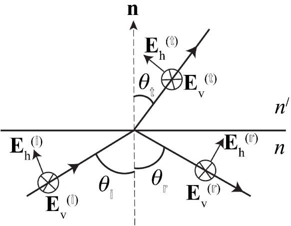
Figure 1:

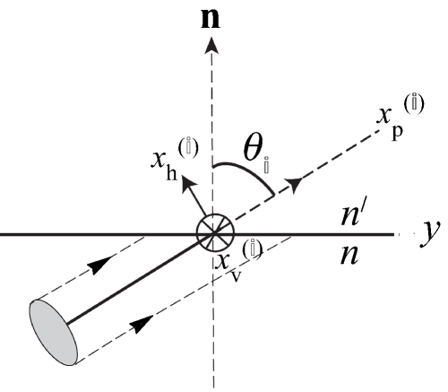
Figure 2:

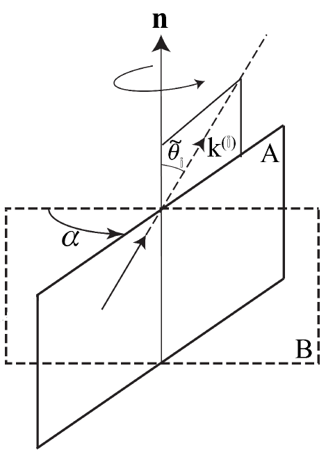
Figure 3:

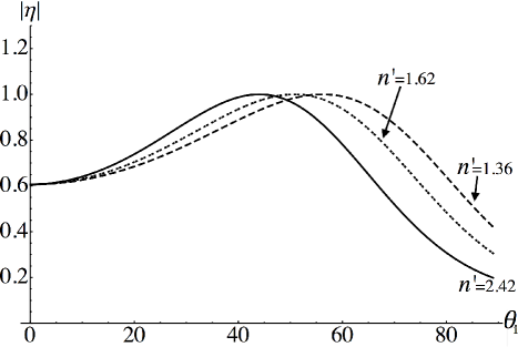
Figure 4:

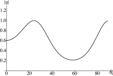
Figure 5:

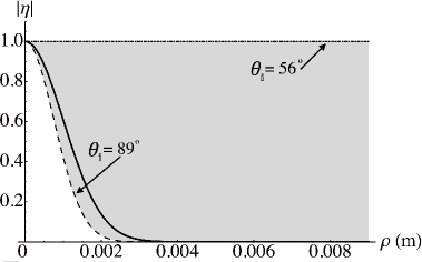
(a)  ethanol ($n^{\prime}=1.36$)

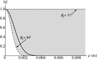
(b)  flint glass ($n^{\prime}=1.62$)

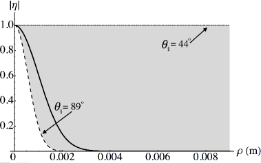
(c)  diamond ($n^{\prime}=2.42$)

Figure 6:

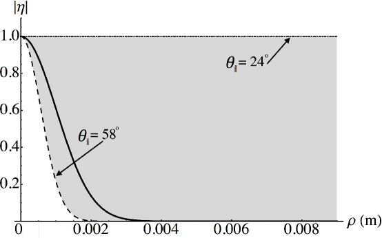
Figure 7: