Evidence of Long Range Order in the Riemann Zeta Function

Abstract

We have done a statistical analysis of some properties of the contour lines Im$(\zeta(s))$ = 0 of the Riemann zeta function. We find that this function is broken up into strips whose average width on the critical line does not appear to vary with height. We also compute the position of the primary zero for the lowest 200 strips, and find that this probability distribution also appears to be scale invariant.

I Introduction

Let $s~{}=~{}\sigma~{}+~{}it$, with $\sigma$ and $t$ real variables. Then for $\sigma~{}>~{}1$ the Riemann zeta function is defined as

$$\zeta(s)~{}=~{}\sum_{n=1}^{\infty}n^{-s}\,.$$ (1)

It follows immediately from Eqn. (1), that for any $t$

$$\lim_{\sigma\to+\infty}\zeta(s)~{}=~{}1\,.$$ (2)

It was shown by RiemannBCRW08 that $\zeta(s)$ can be analytically continued to a function which is meromorphic in the complex plane, that its only divergence is a simple pole at $s$ = 1, and that it has no zeroes on the half-plane $\sigma~{}>~{}1$.

The Riemann HypothesisBCRW08 (RH) is that the only zeroes of $\zeta(s)$ which do not lie on the real axis lie on the critical line $s~{}=~{}{1/2}~{}+~{}it$. It has resisted rigorous proof for over 150 years, and is now widely considered to be the most important unsolved problem in mathematics.Con03 The significance of RH for physics has been shown by many authors.BK99 ; ST08 ; MDMSWS10 ; SH11 ; FHK12

In this work we will study the statistical properties of the contour lines Im$(\zeta(s))$ = 0. We will find that there appears to be a type of long range order in the spacing of these contour lines. We will also find a statistical quantity whose second moment appears to be independent of the height $t$. In other words, this quantity has a scaling exponent of zero, which strongly suggests the existence of some hidden conservation law in $\zeta(s)$.

II Numerical results

The contour lines Im$(\zeta(s))$ = 0 and Re$(\zeta(s))$ = 0 are highly constrained by the Cauchy-Riemann equations. An extensive discussion of their properties, including many illustrations, has been given by Arias de Reyna.Arias03 For this work, the author used the computer program of Collins.Col09 Due to Eqn. (2) and the Cauchy-Riemann equations, there are contour lines Im$(\zeta(s))$ = 0 which break up $\zeta(s)$ into what appear to be essentially horizontal strips, although these contours are not actually straight lines.

If we define the phase $\theta(s)$ by

$$\zeta(s)~{}=~{}|\zeta(s)|\exp(i\theta(s))\,,$$ (3)

then the contour lines at the top and the bottom of each strip have $\cos(\theta)$ = 1, i.e. $\theta$ = 0. Reading the crossings of the critical line, $s$ = 1/2, by these contour lines, we plot the number of strips as a function of the height $t$ in Fig. 1 for the first 200 strips. Because the crossings were measured by eye, the heights were rounded off to integer values. This is merely a rounding error. It does not accumulate. Therefore this rounding error has virtually no effect on the slope of the least squares fitting line shown in Fig. 1.

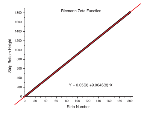
Figure 1: Height of the bottom of a strip (rounded to the nearest integer) on the critical line $\sigma$ = 1/2 as a function of strip number for the first 200 strips.

The linear least squares fit to the data is

$$Y~{}=~{}0.05(9)~{}+~{}9.0646(8)*X\,,$$ (4)

where the numbers in parentheses are the statistical errors in the last significant figure. Since there is a nontrivial distribution of strip widths, there is a small amount of jitter of the data around the fitting line. However, there is absolutely no indication of any curvature in the fit. The bottom of the first strip sits at a height of approximately $t$ = 10. It is therefore somewhat mysterious that the Y-intercept of the fitting line is consistent (within the statistical error) with a value of zero. If one fits the heights of the tops of the strips instead, one finds (unsurprisingly) that the slope of the fitting line is essentially unchanged, but the Y-intercept is now found to be 9.07(9).

For large positive $\sigma$ Eqn. (1) can be approximated by its first two terms. Under this condition

$${\rm Im}(\zeta(s))~{}\approx~{}{\rm Im}(2^{-s})~{}=~{}2^{-\sigma}\sin(\ln(2)t)\,.$$ (5)

Thus the strip boundaries for large positive $\sigma$ and $t>0$ will be

$$t~{}\approx~{}2m\pi/\ln(2)\,,$$ (6)

where the strip number, $m$, is a positive integer. The numerical value of $2\pi/\ln(2)$ is 9.06472… . Assuming the RH is correct, it seems a reasonable conjecture that the strips remain essentially horizontal for any value of $t$ when $\sigma>0$, which implies that the slope of the least squares fit for the heights of the bottom of each strip will be independent of $\sigma$. The author sees no reason, however, why the Y-intercept of this fit should be independent of $\sigma$. In fact, it appears that for $\sigma<0$ this Y-intercept becomes clearly greater than zero.

The reader should note that, since the sum on the right hand side of Eqn. (1) does not even converge for $\sigma$ = 1/2, it is quite remarkable for the data taken on the critical line, shown in Fig. 1, to be well fit by a straight line with a slope of $2\pi/\ln(2)$. Based on the analysis of Berry and Keating,BK99 for example, one might have expected to see oscillations about this line coming from the higher order terms of the sum.

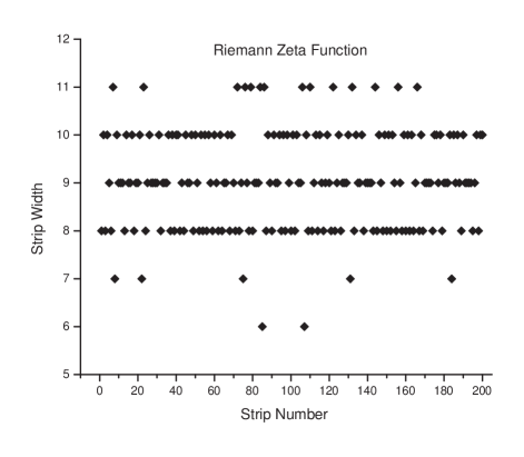
Figure 2: Strip width (rounded to integer values) on the critical line $\sigma$ = 1/2 as a function of strip number, for the first 200 strips.

The strip widths, measured at $\sigma$ = 1/2, as a function of strip number are shown in Fig. 2. As mentioned above, in the process of measuring by eye, these widths were rounded off to integer values. The distribution of strip widths appears to be independent of height. Due to the measurement process, we cannot determine how well this distribution would be fit by a Poisson distribution. There is a clear tendency for the distribution to become narrower as $\sigma$ becomes greater than 1, i.e. the narrow strips become wider and the wide strips become narrower. It would be interesting to calculate the analytical form of this distribution for large positive $\sigma$.

The reader should note that Arias de ReynaArias03 displays a few strips near the critical line at much greater values of $t$ than those studied here, and the widths of those strips are consistent with our estimates of the widths for $t~{}<~{}2000$.

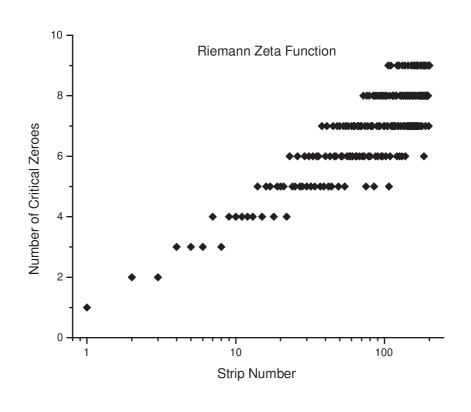
Figure 3: Number of critical zeroes in a strip versus strip number, for the first 200 strips. The $X$-axis is scaled logarithmically.

The number of critical zeroes in a strip versus strip height is shown in Fig. 3. We see that the number of zeroes increases approximately logarithmically with strip number. Because we saw in Fig. 1 and Fig. 2 that the distribution of strip widths appears to be independent of the strip number, this is unsurprising. It has been known for many years that the density of the critical zeroes increases approximately as $\log(t)$. Actually, the average density of critical zeroes as a function of $t$ is known to a much greater precision than this.Arias03

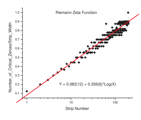
Figure 4: (Number of zeroes on the strip)/(strip width) versus strip number, for the first 200 strips. The $X$-axis is scaled logarithmically.

The width of each strip on the line $\sigma$ = 1/2 is highly correlated with the number of zeroes in the strip. To see this, in Fig. 4 we display the function (number of zeroes on the strip) divided by (strip width) versus the strip number. Comparing Fig. 4 to Fig. 3, it is clear that the scatter in Fig. 4 is much smaller. This is true despite the large roundoff error in our measurement of the strip width.

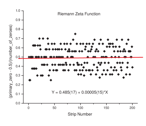
Figure 5: (Number of the primary zero $-~{}0.5$)/(Number of zeroes) versus strip number, for the first 200 strips.

Due to the requirements of the Cauchy-Riemann equations, in each strip there is one special zero, which we will call the primary zero. Each primary zero has the property that the contour with phase $\theta$ = 0 going out of it extends to $\sigma~{}=~{}+\infty$, at a height

$$t~{}\approx~{}(2m+1)\pi/\ln(2)\,.$$ (7)

For all the other critical zeroes, the contour with phase $\theta~{}=~{}0$ goes to $\sigma~{}=~{}-\infty$.

One can now ask the question “Where is the primary zero located in the strip?” It seems obvious, by reason of symmetry, that the average position of the primary zero should be at the center of the strip. However, there is no symmetry reason why the probability distribution for the primary zero should be uniform. In Fig. 5 we display the values for the function (number of the primary zero (counting from the bottom of the strip) $-~{}0.5$) divided by (number of zeroes in the strip) versus the strip number. The subtraction of 0.5 in the numerator is necessary so that this function has the value 0.5 when the primary zero is the middle zero.

The linear least squares fit to the data of Fig. 5 shows that the average position of the primary zero is indeed at the center of the strip. Remarkably, one sees that the value of the variance of this probability distribution seems to be independent of the strip height. This observation is confirmed by comparing the variance for the first 100 strips with the variance for the second 100 strips.

If this probability distribution remains nontrivial (i.e. neither becoming uniform nor collapsing) in the limit $t\to\infty$, then we must conclude that all of the zeroes in a strip are highly correlated with each other. Since the number of zeroes in a strip is expected to diverge as $t\to\infty$, this is a very interesting effect. It strongly suggests that there must exist some unknown (to the author) symmetry or hidden conservation law at work.

III Summary

In this work we have done a statistical analysis of some properties of the contour lines of the Riemann zeta function. We have uncovered some amazing and previously unknown facets of the behavior of this remarkable function.

- (1) The Riemann Hypothesis, edited by P. Borwein, S. Choi, B. Rooney and A. Weirathmueller (Springer, New York, 2008).
- (2) J. B. Conrey, Notices Amer. Math. Soc. 50, 341 (2003).
- (3) M. V. Berry and J. P. Keating, SIAM Rev. 41, 236 (1999).
- (4) G. Sierra and P. K. Townsend, Phys. Rev. Lett. 101, 110201 (2008).
- (5) R. Mack et al., Phys. Rev. A 82, 032119 (2010).
- (6) D. Shumayer and D. A. W. Hutchinson, Rev. Mod. Phys. 83, 307 (2011).
- (7) Y. V. Fyodorov, G. A. Hiary and J. P. Keating, Phys. Rev. Lett. 108, 170601 (2012).
- (8) J. Arias de Reyna, arXiv:math/0309433v1 (2003).
- (9) B. Collins, Contour Plots of the Zeta Function from the Wolfram Demonstrations Project, http://demonstrations.wolfram.com/ContourPlotsOfTheZetaFunction/ (2009).