Nature of Lyman Alpha Blobs: Powered by Extreme Starbursts

Abstract

We present a new model for the observed Ly$\alpha$ blobs (LABs) within the context of the standard cold dark matter model. In this model, LABs are the most massive halos with the strongest clustering (proto-clusters) undergoing extreme starbursts in the high-z universe. Aided by calculations of detailed radiative transfer of ${\rm Ly}\alpha$ photons through ultra-high resolution ($159$pc) large-scale ($\geq 30$Mpc) adaptive mesh-refinement cosmological hydrodynamic simulations with galaxy formation, this model is shown to be able to, for the first time, reproduce simultaneously the global ${\rm Ly}\alpha$ luminosity function and luminosity-size relation of the observed LABs. Physically, a combination of dust attenuation of ${\rm Ly}\alpha$ photons within galaxies, clustering of galaxies, and complex propagation of ${\rm Ly}\alpha$ photons through circumgalactic and intergalactic medium gives rise to the large sizes and frequently irregular isophotal shapes of LABs that are observed. A generic and unique prediction of this model is that there should be strong far-infrared (FIR) sources within each LAB, with the most luminous FIR source likely representing the gravitational center of the proto-cluster, not necessarily the apparent center of the ${\rm Ly}\alpha$ emission of the LAB or the most luminous optical source. Upcoming ALMA observations should unambiguously test this prediction. If verified, LABs will provide very valuable laboratories for studying formation of galaxies in the most overdense regions of the universe at a time when global star formation is most vigorous.

1 Introduction

The physical origin of spatially extended (tens to hundreds of kiloparsecs) luminous (${\rm L_{Ly\alpha}}\geq 10^{43}$erg/s) Ly$\alpha$ sources, also known as Ly$\alpha$ blobs (LABs) first discovered more than a decade ago (e.g., Francis et al., 1996; Fynbo et al., 1999; Keel et al., 1999; Steidel et al., 2000), remains a mystery. By now several tens of LABs have been found (e.g., Matsuda et al., 2004; Dey et al., 2005; Saito et al., 2006; Smith et al., 2009; Matsuda et al., 2011). One fact that has confused the matter considerably is that they appear to be associated with a very diverse galaxy population, including regular Lyman break galaxies (LBGs) (e.g., Matsuda et al., 2004), ultra-luminous infrared galaxies (ULIRGs) and sub-millimeter galaxies (SMGs) (e.g., Chapman et al., 2001; Geach et al., 2005, 2007; Matsuda et al., 2007; Yang et al., 2011b), unobscured (e.g., Bunker et al., 2003; Weidinger et al., 2004) and obscured quasars (e.g., Basu-Zych & Scharf, 2004; Geach et al., 2007; Smith et al., 2009), or either starbursts or obscured quasars (e.g., Geach et al., 2009; Scarlata et al., 2009; Colbert et al., 2011). An overarching feature, however, is that the vast majority of them are associated with massive halos or rich large-scale structures that reside in dense parts of the Universe and will likely evolve to become rich clusters of galaxies by $z=0$ (e.g., Steidel et al., 2000; Chapman et al., 2004; Matsuda et al., 2004; Palunas et al., 2004; Matsuda et al., 2006; Prescott et al., 2008; Matsuda et al., 2009; Yang et al., 2009; Webb et al., 2009; Weijmans et al., 2010; Matsuda et al., 2011; Erb et al., 2011; Yang et al., 2011a; Zafar et al., 2011). Another unifying feature is that LABs are strong infrared emitters. For instance, most of the 35 LABs with size $>30$ kpc identified by Matsuda et al. (2004) in the SSA 22 region have been detected in deep Spitzer observations (Webb et al., 2009).

Many physical models of LABs have been proposed. A leading contender is the gravitational cooling radiation model in which gas that collapses inside a host dark matter halo releases a significant fraction of its gravitational binding energy in Ly$\alpha$ line emission (e.g., Haiman et al., 2000; Fardal et al., 2001; Birnboim & Dekel, 2003; Dijkstra et al., 2006; Yang et al., 2006; Dijkstra & Loeb, 2009; Goerdt et al., 2010; Faucher-Giguère et al., 2010; Rosdahl & Blaizot, 2012). The strongest observational support for this model comes from two LABs that appear not to be associated with any strong AGN/galaxy sources (Nilsson et al., 2006; Smith et al., 2008), although lack of sub-mm data in the case of Nilsson et al. (2006) and a loose constraint of $\leq 550{\rm\,M_{\odot}}$yr^-1 ($3\sigma$) in the case of Smith et al. (2008) both leave room to accommodate AGN/galaxies powered models. Another tentative support is claimed to come from the apparent positive correlation between velocity width (represented by the full width at half maximum, or FWHM, of the line) and Ly$\alpha$ luminosity (Saito et al., 2008), although the observed correlation FWHM $\propto{\rm L_{Ly\alpha}}$ appears to be much steeper than expected (approximately) FWHM $\propto{\rm L_{Ly\alpha}}^{1/3}$ for virialized systems. Other models include photoionization of cold dense, spatially extended gas by obscured quasars (e.g., Haiman & Loeb, 2001; Geach et al., 2009), by population III stars (e.g., Jimenez & Haiman, 2006), or by spatially extended inverse Compton X-ray emission (e.g., Scharf et al., 2003), emission from dense, cold superwind shells (e.g., Taniguchi & Shioya, 2000; Ohyama et al., 2003; Mori et al., 2004; Wilman et al., 2005; Matsuda et al., 2007), or a combination of photoionization and gravitational cooling radiation (e.g., Furlanetto et al., 2005).

The aim of this writing is, as a first step, to explore a simple star formation based model in sufficient details to access its physical plausibility and self-consistency, through detailed ${\rm Ly}\alpha$ radiative transfer calculations utilizing a large set of massive ($\geq 10^{12}{\rm\,M_{\odot}}$) starbursting galaxies from an ultra-high resolution ($\sim 110h^{-1}$pc), cosmological, adaptive mesh refinement (AMR) hydrodynamic simulation at $z=3.1$. The most critical, basically the only major, free parameter in our model is the magnitude of dust attenuation. Adopting the observationally motivated trend that higher SFR galaxies have higher dust attenuation, with an overall normalization that seems plausible (e.g., we assume that $\sim 5$% of ${\rm Ly}\alpha$ photons escape a galaxy of ${\rm SFR}=100{\rm\,M_{\odot}}$ yr^-1), the model can successfully reproduce the global ${\rm Ly}\alpha$ luminosity function and the luminosity-size relation of LABs. To our knowledge this is the first model that is able to achieve this. The precise dependence of dust attenuation on SFR is not critical, within a reasonable range, and hence the results are robust.

In this model we show that LABs at high redshift correspond to proto-clusters containing the most massive galaxies/halos in the universe. Within each proto-cluster, all member galaxies contribute collectively to the overall ${\rm Ly}\alpha$ emission, giving rise to the diverse geometries of the apparent contiguous large-area LAB emission, which is further enhanced by projection effects due to other galaxies that are not necessarily in strong gravitational interactions with the main galaxy (or galaxies), given the strong clustering environment of massive halos in a hierarchical universe. This prediction that LABs should correspond to the most overdense regions in the universe at high redshift is fully consistent with the observed universal association of LABs with high density peaks (see references above). The relative contribution to the overall ${\rm Ly}\alpha$ emission from each individual galaxy depends on a number of variables, including dust attenuation of ${\rm Ly}\alpha$ photons within the galaxy and propagation and diffusion processes through its complex circumgalactic medium and the intergalactic medium. Another major predictions of this model is that a large fraction of the stellar (and AGN) optical and ultraviolet (UV) radiation (including Ly$\alpha$ photons) is reprocessed by dust and emerges as infrared (IR) radiation, consistent with observations of ubiquitous strong infrared emission from LABs. We should call this model simply “starburst model” (SBM), encompassing those with or without contribution from central AGNs. This model automatically includes emission contribution from gravitational cooling radiation, which is found to be significant but sub-dominant compared to stellar radiation. Interestingly, we also find that ${\rm Ly}\alpha$ emission originating from nebular emission (rather than the stellar emission), which includes contribution from gravitational binding energy due to halo collapse, is more centrally concentrated than that from stars.

One potentially very important prediction is that in this model the Ly$\alpha$ emission from photons that escape to us is expected to contain significant polarization signals. Although polarization radiative transfer calculations will be performed to detail the polarization signal in a future study, we briefly elaborate the essential physics and latest observational advances here. One may broadly file all the proposed models into two classes in terms of the spatial distribution of the underlying energy source: central powering or in situ. Starburst galaxy and AGN powered models belong to the former, whereas gravitational cooling radiation model belongs to the latter. A smoking gun test between these two classes of models is the polarization signal of the Ly$\alpha$ emission. In the case of a central powering source (not necessarily a point source) the Ly$\alpha$ photons diffuse out, spatially and in frequency, through optically thick medium and escape by a very large number of local resonant scatterings in the Ly$\alpha$ line profile core and a relatively smaller number of scatterings in the damping wings with long flights. Upon each scattering a Ly$\alpha$ photon changes its direction, location and frequency, dependent upon the geometry, density and kinematics of the scattering neutral hydrogen atoms. In idealized models with central powering significant linear polarizations of tens of percent on scales of tens to hundreds of kiloparsecs are predicted and the polarization signal strength increases with radius (e.g., Lee & Ahn, 1998; Rybicki & Loeb, 1999; Dijkstra & Loeb, 2008). On the other hand, in situ radiation from the gravitational cooling model is not expected to have significant polarizations (although detailed modeling will be needed to quantify this) or any systematic radial trend, because thermalized cooling gas from (likely) filaments will emit Ly$\alpha$ photons that are either not scattered significantly or have no preferential orientation or impact angle with respect to the scattering medium.

An earlier attempt to measure polarization of LABd05 at $z=2.656$ produced a null detection (Prescott et al., 2011). A more recent observation by Hayes et al. (2011), for the first time, detected a strong polarization signal tangentially oriented (almost forming a complete ring) from LAB1 at $z=3.05$, whose strength increases with radius from the LAB center, a signature that is expected from central powering; they found the polarized fraction (P) of 20 percent at a radius of 45 kpc. Hayes et al. (2011) convincingly demonstrate their detection and, at the same time, explain the consistency of their result with the non-detection by Prescott et al. (2011), if the emission from LABd05 is in fact polarized, thanks to a significant improvement in sensitivity and spatial resolution in Hayes et al. (2011). This latest discovery lends great support to models with central powering, including SBM, independent of other observational constraints that may or may not differentiate between the two classes of models or between models in each class. But we stress that detailed polarization calculations will be needed to enable statistical comparisons.

The outline of this paper is as follows. In §2.1 we detail simulation parameters and hydrodynamics code, followed by a description of our Ly$\alpha$ radiative transfer method in §2.2. Results are presented in §3 with conclusions given in §4.

2 Simulations

2.1 Hydrocode and Simulation Parameters

We perform cosmological simulations with the AMR Eulerian hydro code, Enzo (Bryan & Norman, 1999; Joung et al., 2009). First we ran a low resolution simulation with a periodic box of $120~{}h^{-1}$Mpc (comoving) on a side. We identified a region centered on a cluster of mass of $\sim 3\times 10^{14}{\rm\,M_{\odot}}$ at $z=0$. We then resimulate with high resolution of the chosen region embedded in the outer $120h^{-1}$Mpc box to properly take into account large-scale tidal field and appropriate boundary conditions at the surface of the refined region. The refined region has a comoving size of $21\times 24\times 20h^{-3}$Mpc³ and represents $1.8\sigma$ matter density fluctuation on that volume. The dark matter particle mass in the refined region is $1.3\times 10^{7}h^{-1}{\rm\,M_{\odot}}$. The refined region is surrounded by three layers (each of $\sim 1h^{-1}$Mpc) of buffer zones with particle masses successively larger by a factor of $8$ for each layer, which then connects with the outer root grid that has a dark matter particle mass $8^{4}$ times that in the refined region. We choose the mesh refinement criterion such that the resolution is always better than $111h^{-1}$pc (physical), corresponding to a maximum mesh refinement level of $13$ at $z=0$. The simulations include a metagalactic UV background (Haardt & Madau, 1996), and a model for shielding of UV radiation by neutral hydrogen (Cen et al., 2005). They include metallicity-dependent radiative cooling (Cen et al., 1995). Our simulations also solve relevant gas chemistry chains for molecular hydrogen formation (Abel et al., 1997), molecular formation on dust grains (Joung et al., 2009), and metal cooling extended down to $10~{}$K (Dalgarno & McCray, 1972). Star particles are created in cells that satisfy a set of criteria for star formation proposed by Cen & Ostriker (1992). Each star particle is tagged with its initial mass, creation time, and metallicity; star particles typically have masses of $\sim$$10^{6}{\rm\,M_{\odot}}$.

Supernova feedback from star formation is modeled following Cen et al. (2005). Feedback energy and ejected metal-enriched mass are distributed into 27 local gas cells centered at the star particle in question, weighted by the specific volume of each cell, which is to mimic the physical process of supernova blastwave propagation that tends to channel energy, momentum and mass into the least dense regions (with the least resistance and cooling). We allow the entire feedback processes to be hydrodynamically coupled to surroundings and subject to relevant physical processes, such as cooling and heating. The total amount of explosion kinetic energy from Type II supernovae for an amount of star formed $M_{*}$ with a Chabrier initial mass function (IMF) is $e_{SN}M_{*}c^{2}$ (where $c$ is the speed of light) with $e_{SN}=6.6\times 10^{-6}$. Taking into account the contribution of prompt Type I supernovae, we use $e_{SN}=1\times 10^{-5}$ in our simulations. Observations of local starburst galaxies indicate that nearly all of the star formation produced kinetic energy is used to power galactic superwinds (e.g., Heckman, 2001). Supernova feedback is important primarily for regulating star formation and for transporting energy and metals into the intergalactic medium. The extremely inhomogeneous metal enrichment process demands that both metals and energy (and momentum) are correctly modeled so that they are transported in a physically sound (albeit still approximate at the current resolution) way. The kinematic properties traced by unsaturated metal lines in damped Lyman-alpha systems (DLAs) are extremely tough tests of the model, which is shown to agree well with observations (Cen, 2012b).

We use the following cosmological parameters that are consistent with the WMAP7-normalized (Komatsu et al., 2010) $\Lambda$CDM model: $\Omega_{M}=0.28$, $\Omega_{b}=0.046$, $\Omega_{\Lambda}=0.72$, $\sigma_{8}=0.82$, $H_{0}=100h\,{\rm km\,s}^{-1}{\rm Mpc}^{-1}=70\,{\rm km\,s}^{-1}{\rm Mpc}^{-1}$ and $n=0.96$. This simulation has been used (Cen, 2011b) to quantify partitioning of stellar light into optical and infrared light, through ray tracing of continuum photons in a dusty medium that is based on self-consistently computed metallicity and gas density distributions.

We identify galaxies in our high resolution simulations using the HOP algorithm (Eisenstein & Hu, 1999), operated on the stellar particles, which is tested to be robust and insensitive to specific choices of concerned parameters within reasonable ranges. Satellites within a galaxy are clearly identified separately. The luminosity of each stellar particle at each of the Sloan Digital Sky Survey (SDSS) five bands is computed using the GISSEL stellar synthesis code (Bruzual & Charlot, 2003), by supplying the formation time, metallicity and stellar mass. Collecting luminosity and other quantities of member stellar particles, gas cells and dark matter particles yields the following physical parameters for each galaxy: position, velocity, total mass, stellar mass, gas mass, mean formation time, mean stellar metallicity, mean gas metallicity, star formation rate, luminosities in five SDSS bands (and various colors) and others. At a spatial resolution of $159$pc (physical) with nearly 5000 well resolved galaxies at $z\sim 3$, this simulated galaxy catalog presents an excellent (by far, the best available) tool to study galaxy formation and evolution.

2.2 ${\rm Ly}\alpha$ Radiative Transfer Calculation

The AMR simulation resolution is $159$pc at $z=3$. For each galaxy we produce a cylinder of size $(2R_{\rm vir})\times(2R_{\rm vir})\times(42R_{\rm vir})$ on a uniform grid of cell size $318$pc, where $R_{\rm vir}$ is the virial radius of the host halo. The purpose of using the elongated geometry is to incorporate the line-of-sight structures. Subsequently, in our ${\rm Ly}\alpha$ radiative transfer calculation, the line-of-sight direction is set to be along the longest dimension of the cylinder. In each cell of a cylinder ${\rm Ly}\alpha$ photon emissivities are computed, separately from star formation and cooling radiation. The luminosity of ${\rm Ly}\alpha$ produced by star formation is computed as ${\rm L_{Ly\alpha}}=10^{42}[{\rm SFR}/({\rm\,M_{\odot}}{\rm yr}^{-1})]\,{\rm erg\,s^{-1}}$ (Furlanetto et al., 2005), where SFR is the star formation rate in the cell. The ${\rm Ly}\alpha$ emission from cooling radiation is computed with the gas properties in the cell by following the rates of excitation and ionization.

With ${\rm Ly}\alpha$ emissivity, neutral hydrogen density, temperature, and velocity in the simulations, a Monte Carlo code (Zheng & Miralda-Escudé, 2002) is adopted to follow the ${\rm Ly}\alpha$ radiative transfer. The code has been recently used to study ${\rm Ly}\alpha$ emitting galaxies (Zheng et al., 2010, 2011a, 2011b). In our radiative transfer calculation, the number of ${\rm Ly}\alpha$ photons drawn from a cell is proportional to the total ${\rm Ly}\alpha$ luminosity in the cell, with a minimum number of 1000, and each photon is given a weight in order to reproduce the luminosity of the cell. ${\rm Ly}\alpha$ photons associated with star formation and cooling radiation are tracked separately so that we can study their final spatial distributions. For each photon, the scattering with neutral hydrogen atoms and the subsequent changes in frequency, direction, and position are followed until it escapes from the simulation cylinder. More details about the code can be found in Zheng & Miralda-Escudé (2002) and Zheng et al. (2010).

The pixel size of the ${\rm Ly}\alpha$ images from the radiative transfer calculation is chosen to be equal to $318$pc, corresponding to $0.04\arcsec$. We smooth the ${\rm Ly}\alpha$ images with 2D Gaussian kernels to match the resolutions in Matsuda et al. (2011) for detecting and characterizing LABs from observation. In Matsuda et al. (2011), the area of an LAB is the isophotal area with a threshold surface brightness $1.4\times 10^{-18}{\rm erg\,s^{-1}cm^{-2}arcsec^{-2}}$ in the narrowband image smoothed to an effective seeing of FWHM 1.4$\arcsec$ (slightly different from Matsuda et al. 2004, where FWHM=1$\arcsec$), while the ${\rm Ly}\alpha$ luminosity is computed with the isophotal aperture in the FWHM=1$\arcsec$ image. We define LABs in our model by applying a friends-of-friends algorithm to link the pixels above the threshold surface brightness in the computed ${\rm Ly}\alpha$ images, with the area and luminosity computed from smoothed images with FWHM=1.4$\arcsec$ and FWHM=1$\arcsec$, respectively.

3 Results

The SBM model that we study here in great detail may appear at odds with available observations at first sight. In particular, the LABs often lack close correspondence with galaxies in the overlapping fields and their centers are often displaced from the brightest galaxies in the fields. As we show below, these puzzling features are in fact exactly what are expected in the SBM model. The reasons are primarily three-fold. First, LABs universally arise in large halos with a significant number of galaxies clustered around them. Second, dust attenuation renders the amount of Ly$\alpha$ emission emerging from a galaxy dependent substantially sub-linearly on star formation rate. Third, the observed Ly$\alpha$ emission, in both amount and three-dimensional (3D) location, originating from each galaxy depends on complex scattering processes subsequently.

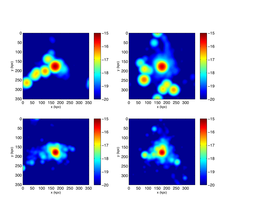
Figure 1: Two examples: left (a) and right (b) columns. See the caption below with columns (c) and (d).

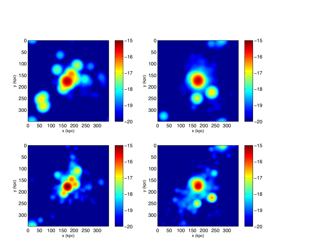
Figure 1: Two more examples: left (c) and right (d) columns. The four columns (a,b,c,d) show the logarithm of Ly$\alpha$ surface brightness maps (in units of ${\rm erg\,s^{-1}cm^{-2}arcsec^{-2}}$) for four randomly selected large galaxies of virial masses both exceeding $10^{12}{\rm\,M_{\odot}}$ at $z=3.1$ with the primary galaxy centered on their respective panel. For each column the bottom panel is obtained, if one only includes galaxies within $\pm R_{\rm vir}$ of the primary galaxy along the line of sight, where $R_{\rm vir}$ is the virial radius of the primary galaxy. The top panel is obtained, including all galaxies within $\pm 10h^{-1}$Mpc comoving of the primary galaxy along the line of sight. The length shown is in physical kpc. The effects of dust and faint sources have not been included yet in these plots (see the text for more details).

3.1 Effects Caused by Galaxy Clustering

We find that large-scale structure and clustering of galaxies play a fundamental role in shaping all aspects of LABs, including two-dimensional line-of-sight velocity structure, line profile and ${\rm Ly}\alpha$ image in the sky plane. To illustrate this, Figure 1 shows Ly$\alpha$ surface brightness maps (after the radiative transfer calculation) for four randomly selected galaxies with virial mass of the central galaxy exceeding $10^{12}{\rm\,M_{\odot}}$ at $z=3.1$. We find that Ly$\alpha$ emission stemming from stellar radiation dominate over the gas cooling by about 10:1 to 4:1 in all relevant cases. We also find that the Ly$\alpha$ emission due to gas cooling is at least as centrally concentrated as from the stellar emission for each galaxy. From this figure it has become clear that large-scale structure and projection effects are instrumental to rendering the appearance of LABs in all aspects (image as well as spectrum). One could see that, for example in the top-left panel of Figure 1, the approximately linear structure aligned in the direction of lower-left to upper-right is composed of three additional galaxies that are well outside the virial radius of the primary galaxy but from projected structures. At the $1.4\times 10^{-18}{\rm erg\,s^{-1}cm^{-2}arcsec^{-2}}$ detection isophotal contours of Matsuda et al. (2004) and Matsuda et al. (2011) for LABs, the entire linear structure may be identified as a single LAB. This rather random example is strikingly reminiscent of the observed LAB structures (e.g., Matsuda et al., 2009; Erb et al., 2011; Yang et al., 2011a). Interestingly, depending on which galaxy is brighter and located on the front or back, the overall Ly$\alpha$ emission of the LAB may show a variety of line profiles. For example, it could easily account for a broad/brighter blue side in the line profile, as noted by Saito et al. (2006) for some of the observed LABs, which was originally taken as supportive evidence for the gravitational cooling radiation model. Furthermore, it is not difficult to envision that the overall velocity width of an LAB does not necessarily reflect the virial velocity of a virialized system and may display a wide range from small (masked by caustics effect) to large (caused by either large virial velocities, infall velocities, or Hubble expansion). A detailed spectral analysis will be presented elsewhere.

For the results shown in Figure 1 we have not included dust effect, contributions from small galaxies ($M_{h}<10^{9.5}{\rm\,M_{\odot}}$) that are not properly captured in our simulation due to finite resolution, and instrumental noise. We now describe how we include these important effects.

3.2 Taking into Account Faint, Under-resolved Sources

Although the resolution of our simulations is high, it is still finite and small sources are incomplete. We find that the star formation rate (SFR) function in the simulation flattens out at 3${\rm\,M_{\odot}}\,{\rm yr}^{-1}$ toward lower SFR at $z=2-3$ (Cen, 2011b), which likely means that sources with SFR$<3{\rm\,M_{\odot}}\,{\rm yr}^{-1}$ are unresolved/under-resolved and hence incomplete in the simulations. Since these low SFR sources that cluster around large galaxies contribute to the ${\rm Ly}\alpha$ emission of LABs, it is necessary to include them in our modeling. For this purpose, we need to sample their SFR distribution and spatial distribution inside halos.

First, we need to model the luminosity or SFR distribution of the faint, unresolved sources. In each LAB-hosting halo in the simulations, the number of (satellite) sources with SFR$>$3${\rm\,M_{\odot}}\,{\rm yr}^{-1}$ is found to be proportional to the halo mass $M_{h}$. Observationally, the faint end slope $\alpha$ of the UV luminosity function of star forming galaxies is $\sim-1.8$ (e.g., Reddy & Steidel, 2009). Given this faint end slope, the contribution due to faint, unresolved sources is weakly convergent. As a result, the overall contribution from faint sources do not strongly depend on the faint limit of the correction procedure. We find that the conditional SFR function $\phi(L;M_{h})$ of faint sources (SFR$<3{\rm\,M_{\odot}}\,{\rm yr}^{-1}$) in halos can be modeled as

$$\phi(L;M_{h})=\frac{dN(M_{h})}{dL}=\frac{-(\alpha+1)}{L_{\rm th}}\left(\frac{L}{L_{\rm th}}\right)^{\alpha}\frac{M_{h}}{M_{1}},$$ (1)

where $L$ represents the SFR and $L_{\rm th}=3{\rm\,M_{\odot}}\,{\rm yr}^{-1}$, $\alpha=-1.8$, and $M_{1}=10^{12}{\rm\,M_{\odot}}$. This conditional SFR function allows us to draw SFR for faint sources to be added in our model.

We now turn to the spatial distribution of faint sources. In the simulation the spatial distribution (projected to the sky plane) of satellite sources in halos is found to closely follow a power-law with a slope of $-2$. This is in good agreement with the observed small scale slope of the projected two-point correlation function of LBGs (Ouchi et al., 2005). There is some direct observational evidence that there are faint UV sources distributed within the LAB radii. Matsuda et al. (2012) perform stacking analysis of $z\sim 3.1$ ${\rm Ly}\alpha$ emitters and protocluster LBGs, showing diffuse ${\rm Ly}\alpha$ profile in the stacked ${\rm Ly}\alpha$ image. Interestingly, the profiles in the stacked UV images appear to be extended to scales of tens of kpc (physical) for the most luminous ${\rm Ly}\alpha$ sources or for sources in protoclusters, suggesting contributions from faint, starforming galaxies.

We add the contribution from faint sources to post-processed unsmoothed ${\rm Ly}\alpha$ images from radiative transfer modeling as follows. For each model LAB, we draw the number and SFRs of faint sources in the range of 0.01–3${\rm\,M_{\odot}}{\rm yr}^{-1}$ based on the conditional SFR distribution in equation (1). Then we distribute them in the unsmoothed ${\rm Ly}\alpha$ image in a radial range of 0.01–1$R_{\rm vir}$ by following the power-law distribution with slope $-2$. The faint sources can be either added as point or extended sources in ${\rm Ly}\alpha$ emission. If added as point sources, they would be smoothed with a 2D Gaussian kernel of FWHM=1.4$\arcsec$ or 1$\arcsec$ when defining LAB size and luminosity. In our fiducial model, each faint source is added as an exponential disk with scale length of 3$\arcsec$ to approximate the radiative transfer effect, which is consistent with the observed diffuse emission profile of star-forming galaxies (Steidel et al., 2011). We find that our final conclusion does not sensitively depend on our choice of the faint source ${\rm Ly}\alpha$ profile.

In Figure 2, panel (a) shows the surface brightness and the $1.4\times 10^{-18}{\rm erg\,s^{-1}cm^{-2}arcsec^{-2}}$ isphotal contour for a model LAB without including the faint sources, while panel (b) is the case with faint sources. We see that the size of the LAB defined by the isophotal aperture does not change much. If the ${\rm Ly}\alpha$ emission of each faint sources is more concentrated, e.g., close to a point source in the unsmoothed image, the LAB size can increase a little bit. Therefore, in both panels (a) and (b), the size is mainly determined by the central bright source. However, as will be described in the next subsection, including the effect of dust extinction will suppress the contribution of the central source and relatively boost that of the faint sources in determining the LAB size.

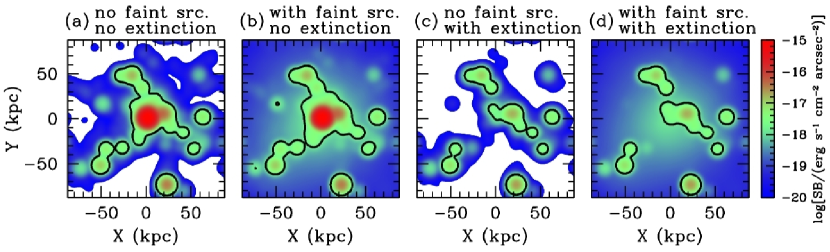
Figure 2: An LAB under different model assumptions. The model LAB shown in this example resides in the most massive host halo in our simulation ($\sim 5\times 10^{12}{\rm\,M_{\odot}}$) at $z=3.1$. The ${\rm Ly}\alpha$ images are smoothed to correspond to seeing of FWHM=1.4$\arcsec$. In each panel, the black contour is the isophotal level of $1.4\times 10^{-18}{\rm erg\,s^{-1}cm^{-2}arcsec^{-2}}$, the surface brightness threshold used in observation to define LABs (Matsuda et al., 2004, 2011). Panels (a)–(d) enumerate the combinations of adding faint sources and extinction. Panel (a) is the initial case without faint sources and without extinction. Panel (d) corresponds to the case with faint sources added and with extinction considered, which we regard as the favored model. See the text for more details.

3.3 Dust Effect

In the cases shown in Figure 1, the central galaxies each have SFR that exceeds $100{\rm\,M_{\odot}}$ yr^-1 and is expected to be observed as a luminous infrared galaxy (LIRG) or ULIRG (Sanders & Mirabel, 1996). This suggests that dust effects are important and have to be taken into account.

In general, there are two types of effects of dust on ${\rm Ly}\alpha$ emission from star-forming galaxies. The first one is related to the production of ${\rm Ly}\alpha$ phtons. Dust attenuates ionizing photons in star-forming galaxies. Since ${\rm Ly}\alpha$ photons come from reprocessed ionizing photons, the attenuation by dust leads to a lower ${\rm Ly}\alpha$ luminosity in the first place. Second, after being produced, ${\rm Ly}\alpha$ photons can be absorbed by dust during propagation. A detailed investigation needs to account for both effects self-consistently, and we reserve that for a future study.

In Cen (2011b) the dust obscuration/absorption is considered in a self-consistent way, with respect to luminosity functions observed in UV and FIR bands. The modelling uses detailed ray tracing with dust obscuration model based on that of our own Galaxy (Draine, 2011) and extinction curve taken from Cardelli et al. (1989). While the simultaneous match of both UV and FIR luminosity functions at $z=2$ without introducing additional free parameters is an important validation of the physical realm of our simulations, it is not necessarily directly extendable to the radiative transfer of ${\rm Ly}\alpha$ photons. Nevertheless, it is reasonable to adopt a simple optical depth approach as follows for our present purpose, normalized by relevant observations, as follows.

For each galaxy we suppress the initial intrinsic Ly$\alpha$ emission, by applying a mapping ${\rm L_{Ly\alpha}}$ to ${\rm L_{Ly\alpha}}\exp{[-\tau({\rm SFR})]}$, where the “effective” optical depth $\tau({\rm SFR})$ is intended to account for extinction of ${\rm Ly}\alpha$ photons as a function of SFR. We stress that this method is approximate and its validation is only reflected by the goodness of our model fitting the observed properties of LABs. We adopt $\tau({\rm SFR})=0.2[{\rm SFR}/({\rm\,M_{\odot}}{\rm yr^{-1}})]^{0.6}$. In reality, in addition, it may be that there is a substantial scatter in $\tau({\rm SFR})$ at a fixed SFR. We ignore such complexities in this treatment. The adopted trend that higher SFR galaxies have larger optical depths is fully consistent with observations (e.g., Nilsson & Møller, 2009). At intrinsic ${\rm SFR}=100{\rm\,M_{\odot}}{\rm yr}^{-1}$ the escaped ${\rm L_{Ly\alpha}}$ luminosity is equivalent to ${\rm SFR}=5{\rm\,M_{\odot}}{\rm yr}^{-1}$, whereas at intrinsic ${\rm SFR}=10{\rm\,M_{\odot}}{\rm yr}^{-1}$ the escaped ${\rm L_{Ly\alpha}}$ luminosity is equivalent to ${\rm SFR}=4.5{\rm\,M_{\odot}}{\rm yr}^{-1}$. It is evident that the scaling of the emerging ${\rm L_{Ly\alpha}}$ luminosity on intrinsic SFR is substantially weakened with dust attenuation. In fact, it may be common that, due to dust effect, the optical luminosity of a galaxy does not necessarily positively correlate with its intrinsic SFR, or the most luminous source in ${\rm Ly}\alpha$ does not necessarily correspond to the highest SFR galaxy within an LAB. As a result, a variety of image appearance and mis-matches between the LAB centers and the most luminous galaxies detected in other bands may result, seemingly consistent with the anecdotal observational evidence mentioned in the introduction.

The effect of dust on the surface brightness distribution for a model LAB is shown in panel (c) of Figure 2. Compared to panel (a), which is the model without dust effect, we see that surface brightness of the central source is substantially reduced and the isophotal area for the threshold $1.4\times 10^{-18}{\rm erg\,s^{-1}cm^{-2}arcsec^{-2}}$ also reduces. The case in panel (c) does not include the contribution from faint sources. In general, taking into account dust effect in our Ly$\alpha$ radiative transfer calculation, the central galaxies tend to make reduced (absolutely and relative to other smaller nearby galaxies) contributions to the Ly$\alpha$ surface brightness maps and in fact the center of each LAB may or may not coincide with the primary galaxy that would likely be a ULIRG in these cases, which is again reminiscent of some observed LABs. In the next subsection, we describe the modeling results of combining all the above effects.

3.4 Final LABs with All Effects Included

By accounting for the line-of-sight structures, the unresolved faint sources, and the dust effect, we find that the observed properties of LABs can be reasonably reproduced by our model.

In panel (d) of Figure 2, we add the faint sources and apply the dust effect. Compared with the case in panel (c), where no faint sources are added, the isophotal area increases. The central source has a substantially reduced surface brightness because of extinction. There appears to be another source near the central source, which corresponds to a source of lower SFR seen in panel (a) but with lower extinction than the central source. From Figure 2, we see that the overall effect is that dust helps reduce the central surface brightness and faint sources help somewhat enlarge the isophotal area.

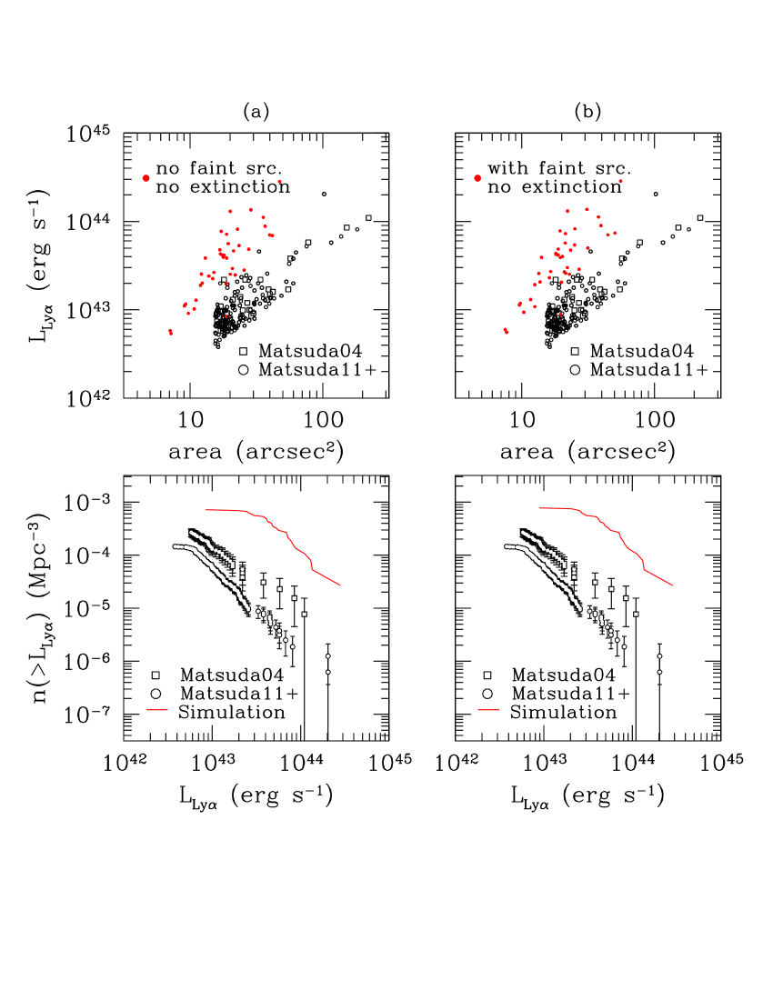
Figure 3: Model predictions under different assumptions along with observed properties of LABs. Top panels show luminosity and size relations and bottom panels cumulative luminosity functions. Panel (a) does not account for dust effect and contributions from faint galaxies under-resolved in our simulation. Panel (b) includes under-resolved sources. Observations are taken from Matsuda et al. (2004) (open squares) and Matsuda et al. (2011) supplemented with new unpublished data (open circles). Model predictions are shown as red points (top panels) and curves (bottom panels).

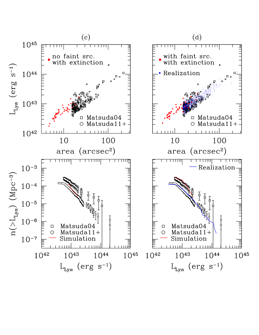
Figure 3: Continued. Panel (c) only includes the dust extinction effect. Panel (d) includes both the dust extinction and the faint sources. The blue dots and blue curve in panel (d) is our realization of the global LF by using the $L_{{\rm Ly}\alpha}-M_{h}$ relation from our model and the analytic halo mass function.

To test the model and see the effect of different assumptions on extinction and faint sources, we compare the model predictions with observational properties of LABs, shown in Figure 3. In the top panels, we compare the luminosity-size relation defined by the isophot with surface brightness $1.4\times 10^{-18}{\rm erg\,s^{-1}cm^{-2}arcsec^{-2}}$. The observed data points are taken from Matsuda et al. (2004) (open squares) and Matsuda et al. (2011) (open circles), which has been supplemented with new, yet unpublished data (Matsuda 2012, private communications). Note that the isophotal area is defined with FWHM=1$\arcsec$ and 1.4$\arcsec$ images in Matsuda et al. (2004) and Matsuda et al. (2011), respectively. This may partly explain that the LAB sizes are somewhat larger with the Matsuda et al. (2011) data points. However, the difference is not substantial. Our model data points follow Matsuda et al. (2011) in defining the luminosity and size.

In the bottom panels of Figure 3, we show the cumulative ${\rm Ly}\alpha$ luminosity function or abundance of LABs. The data points from Matsuda et al. (2004) and Matsuda et al. (2011) (supplemented with new unpublished data; Matsuda 2012, private communications) have a large offset ($\sim$1 dex at the luminous end) from each other, suggesting large sample variance. The survey volumes of Matsuda et al. (2004) and Matsuda et al. (2011) are $1.3\times 10^{5}{\rm Mpc}^{3}$ and $1.6\times 10^{6}{\rm Mpc}^{3}$, respectively. For comparison, the volume of our parent simulation from which we choose our LAB sample is only $3.06\times 10^{4}{\rm Mpc}^{3}$, much smaller than the volume probed by observation.

The red points in top panel (a) of Figure 3 come from our model without extinction and faint sources. Compared to the observational data, the model predicts more or less the correct slope in the luminosity-size relation. However, the overall relation has an offset, which means that the model either overpredicts the luminosity or underpredicts the size, or both. From the bottom panel (a), the model greatly over-predicts the LAB abundance, showing as a vertical shift. But it can also be interpreted as an overprediction of the LAB luminosity, leading to a horizontal shift, which is more likely. Because the central sources are bright, adding faint sources only slightly changes the sizes, as shown in panel (b), which leads to little improvement in solving the mismatches in the luminosity-size relation and in the abundance.

Once the dust extinction effect is introduced, the situation greatly improves. Panel (c) of Figure 3 shows the case with extinction but without adding faint sources. With the extinction included, the luminosity of the predicted LABs drops, and at the same time, the size becomes smaller. Now the model points agree well with observations at the lower end of the range of LAB luminosity ($10^{42.6}-10^{43.3}$erg/s) and size (15-30 arcsec²), the predicted luminosity-size relation conforms to and extends the observed one to still lower luminosity and smaller size. The predicted abundance is much closer to the observed one, as well.

Finally, panel (d) shows the case with both extinction and faint sources included. Adding faint sources helps enlarge the size of an LAB, because faint sources extends the isophot to larger radii. The luminosity also increases by including the contribution from faint sources. As a whole, the model data points appear to slide over the luminosity-size relation towards higher luminosity and larger size. The model luminosity-size relation, although still at the low luminosity end, is fully overlapped with the observed relation. The abundance at the high-luminosity end from the model is within the range probed by observation and shows a similar slope as that in Matsuda et al. (2004). The agreement of the luminosity function between simulations and Matsuda et al. (2004) is largely fortuitous, reflecting that the overall bias of our simulation box over the underlying matter happens to be similar to that of the Matsuda et al. (2004) volume over matter, provided that the model universe is a reasonable statistical representation of the real universe.

Limited by the simulation volume, we are not able to directly simulate the full range of the observed luminosity and size of LABs. Our model, however, reproduces the luminosity-size relation and abundance in the low luminosity end. The most important ingredient in our model to achieve such an agreement with the observation is the dust extinction, which drives the apparent ${\rm Ly}\alpha$ luminosity down into the right range. Accounting for the contribution of faint, unresolved sources in the simulation also plays a role in further enhancing the sizes and, to a less extent, the luminosities of LABs.

To rectify the lack of high luminosity, large size LABs in our simulations due to the limited simulation volume, we perform the following exercise. Figure 4 shows the ${\rm Ly}\alpha$ luminosity and LAB size as a function of halo mass from our model LABs in Figure 3(d). Both quantities correlate with halo mass, but there is a large scatter, which is caused by varying SFRs as well as different environmental effects for halos of a given mass. The largest LABs fall into the range probed by the observational data and they reside in halos above $10^{12}M_{\odot}$. The model suggests that the vast majority of the observed LABs should reside in proto-clusters with the primary halos of mass above $10^{12}M_{\odot}$ at $z\sim 3$ and on average larger LABs correspond to more massive halos. Note that the sources with halo mass below $10^{12}M_{\odot}$ is highly incomplete here. Our results suggest an approximate relation between the halo mass of the central galaxy and the apparent ${\rm Ly}\alpha$ luminosity of the LAB:

$${\rm L_{Ly\alpha}}=10^{42.4}\left({M_{h}\over 10^{12}{\rm\,M_{\odot}}}\right)^{1.15}{\rm erg\,s^{-1}},$$ (2)

which is shown as the solid curve in the left panel of Figure 4. This relation should provide a self-consistency test of our model, when accurate halo masses hosting LABs or spatial clustering of LABs can be measured, interpreted in the context of the $\Lambda$CDM clustering model. We also find that the area-halo mass relation:

$${\rm area}=5.0\left({M_{h}\over 10^{12}{\rm\,M_{\odot}}}\right)^{1.15}{\rm arcsec}^{2},$$ (3)

shown as the solid curve in the right panel of Figure 4. Equations (2) and (3) lead to the following luminosity-size relation

$${\rm area}=5.0\left({{\rm L_{Ly\alpha}}\over{10^{42.4}{\rm erg\,s^{-1}}}}\right){\rm arcsec}^{2},$$ (4)

which matches the observed one, nothing new in this except as a self-consistency check.

Figure 4: Dependence of LAB luminosity and size on halo mass from the model. In each panel, the points are from our model LABs in the simulation. The solid and dotted lines show the relation and scatter we use to populate halos drawn from the analytic halo mass function to compute the expected global ${\rm Ly}\alpha$ LF of LABs. See the text for more details.

By extrapolating the above relations (2,3) to higher halo mass and using the analytic halo mass function (Jenkins et al., 2001), we can obtain the global ${\rm Ly}\alpha$ LF expected from our model. In detail, we draw halo masses based on the analytic halo mass function. For each halo, we compute ${\rm L_{Ly\alpha}}$ from Equation (2). A scatter in $\log{\rm L_{Ly\alpha}}$ is added following a Gaussian distribution with 1$\sigma$ deviation of 0.28dex (indicated by the dotted lines in the left panel of Figure 4). Then Equation (4) is used to assign the area, and a Gaussian scatter of 0.11dex is added to approximately reproduce the scatter seen in the observed luminosity-size relation. The implied scatter in the area-halo mass relation is the sum of the above two scatters in quadrature, i.e., about 0.30 dex, which is indicated by the dotted lines in the right panel of Figure 4. Finally, we adopt the same area cut ($>$15 ${\rm arcsec}^{2}$) used in observations (Matsuda et al., 2011) to define LABs.

Our computed global ${\rm Ly}\alpha$ LF of LABs is shown as the blue curve in the bottom panel (d). The agreement between our predicted global LF and that from the larger-survey-volume observations of Matsuda et al. (2011) is striking. Given still substantial uncertainties involved in our model assumptions, the precise agreement is not to be overstated. However, the fact that the relative displacement between LF from our simulated volume and global LF is in agreement with that between Matsuda et al. (2004) and Matsuda et al. (2011) is quite encouraging, recalling that we have no freedom to adjust any cosmological parameters. This is also indicative of the survey volume of Matsuda et al. (2011) having becoming a fair sample of the universe for LABs in question. The blue dots in top panel (d) show that the predicted luminosity-area relation is simultaneously in agreement with observations, now over the entire luminosity and size range, suggesting that our derived relations in Equations (2), (3), and (4) are statistically applicable to LABs of luminosities higher than those probed by the current simulations.

4 Conclusions and Discussions

We present a new model, termed star-burst model (SBM), for the spatially extended (tens to hundreds of kiloparsecs) luminous (${\rm L_{Ly\alpha}}\gtrsim 10^{43}$erg/s) Ly$\alpha$ blobs. The SBM model is the first model to successfully reproduce both the global ${\rm Ly}\alpha$ luminosity function and the luminosity-size relation of the observed LABs (Matsuda et al., 2004, 2011). In the SBM model ${\rm Ly}\alpha$ emission from both stars and gravitational sources (such as gravitational binding energy released from structure collapse) is included, although it is found that the nebular ${\rm Ly}\alpha$ emission sourced by those other than stars, while significant, is sub-dominant compared to stellar emission. It is also found that ${\rm Ly}\alpha$ emission originating from sources rather than stars is at least as centrally concentrated as that from stars within each galaxy.

Our modeling is based on a high-resolution large-scale cosmological hydrodynamic simulation of structure formation, containing more than $3000$ galaxies with halo mass $M_{h}>10^{10}{\rm\,M_{\odot}}$ and more than $25$ galaxies with $M_{h}>10^{12}{\rm\,M_{\odot}}$ at $z=3.1$, all resolved at a resolution of $159$pc or better. Detailed 3D ${\rm Ly}\alpha$ radiative transfer calculation is applied to sub-volumes centered on each of the 40 most massive star-bursting galaxies in the simulation box with ${\rm SFR}=10-400{\rm\,M_{\odot}}$yr^-1. A self-consistent working model emerges, if proper dust attenuation trend is modeled in that ${\rm Ly}\alpha$ emission from higher SFR galaxies are more heavily attenuated by dust than lower SFR galaxies, which is empirically motivated by observations. For the results shown, we adopt an effective ${\rm Ly}\alpha$ optical depth $\tau({\rm SFR})=0.2[{\rm SFR}/({\rm\,M_{\odot}}{\rm yr^{-1}})]^{0.6}$, which translates to escape fractions of ($5\%$, $45\%$) for ${\rm Ly}\alpha$ photons at ${\rm SFR}=(100,10){\rm\,M_{\odot}}{\rm yr}^{-1}$, respectively. The dust attenuation model has two parameters, a normalization and a powerlaw index. The powerlaw index actually follows the slope of the metal column density dependence on SFR in the simulation. This thus leaves us with the normalization as the only free parameter. In practice, changing the powerlaw index does not sensitively change the results, as long as the normalization is adjusted such that the attenuation at high SFR end ($\sim 100{\rm\,M_{\odot}}$yr^-1) is approximately the same as the adopted value, making the model rather robust.

Also very encouraging is that the model is in broad agreeement with other observed properties of LABs, in addition to the simultaneous reproduction of the observed global ${\rm Ly}\alpha$ luminosity function and the luminosity-size relation aforenoted. Among them, we predict that LABs at high redshift correspond to proto-clusters containing the most massive galaxies/halos in the universe and ubiquitous strong infrared emitters, with the most luminous member galaxies mostly copious in FIR emission, fully consistent with extant observations (e.g., Geach et al., 2007; Bridge et al., 2012). It seems inevitable that some of the galaxies would contain active galactic nuclei (AGN) at the epoch of peak AGN formation in the universe (e.g., Geach et al., 2009). While it is straight-forward to include, the results shown do not include AGN, partly because, to the zero-th order, we may simply “absorb” that by adjusting the dust attenuation effect and partly because observations indicate AGN contribution is subdominant (e.g., Webb et al., 2009; Colbert et al., 2011).

The most massive halos in the standard cold dark matter universe also tend be the most strongly clustered in the universe, among all types of galaxies, and we predict that there should be numerous galaxies clustered around LABs (e.g., Uchimoto et al., 2008). Prescott et al. (2012) use high-resolution Hubble Space Telescope imaging to resolve galaxies within a giant LAB at $z\sim 2.656$. They find many compact, low-luminosity galaxies. Their observation becomes incomplete below $\sim 0.1L^{*}$, and with extrapolation there would be about 80 sources above $0.01L^{*}$ within a radius of 7$\arcsec$. Their LAB has ${\rm L_{Ly\alpha}}=10^{44}{\rm erg\,s^{-1}}$ and an isophotal area $\sim 140\,{\rm arcsec}^{2}$, falling well onto the observed luminosity-size relation shown in Figure 3. Extrapolating from our model, the LAB is predicted to reside in a halo with mass of $\sim 10^{13}M_{\odot}$ (Fig. 4). The number of faint sources within 7$\arcsec$ above $0.01L^{*}$ from our model would be about 100, in agreement with the observation. With the availability of ALMA, observers could make use of its superb capabilities to confirm the generic prediction of this model that there should be FIR sources in each LAB with the most luminous FIR source likely representing the center of the proto-cluster. In combination with optical and other observations, this will potentially provide extremely useful information on the formation of galaxies in the most overdense regions of the universe when star formation is most vigorous and clusters have yet to be assembled.

We highlight here that a potentially very discriminating signature of this model lies in the expected, significant polarization strength of the ${\rm Ly}\alpha$ emission at large scales ($\sim$10−100kpc), which is not expected in some competing models for LABs, such as those sourcing primarily gravitational binding energy on large scales due to massive halo formation. We plan to quantify this signal with detailed polarization radiative transfer calculations of ${\rm Ly}\alpha$ photons.

It is mentioned in passing that our model suggests the trends seen in LABs, in terms of the global ${\rm Ly}\alpha$ luminosity function and the luminosity-size relation of the observed LABs, are continuously extended to less luminous ${\rm Ly}\alpha$ emitters (LAEs). Consequently, we predict that LAEs, less luminous than LABs, have smaller sizes compared to those of LABs at a fixed isophotal level and should also be less strongly clustered than LABs, forming an extension of the observed LAB luminosity-size relation as well as the LAB luminosity and correlation functions.

Finally, it is reassuring to note that the cosmological simulations themselves have already been subject to and passed a range of tests concerning a variety of observables of galaxies and the intergalactic medium, including properties of DLAs at $z=0-4$ (Cen, 2012b), O VI absorbers in the circumgalactic and intergalactic medium in the local universe (Cen, 2012a), global evolution of star formation rate density and cosmic downsizing of galaxies (Cen, 2011a), galaxy luminosity functions from $z=0$ to $z=3$ (Cen, 2011a, b), and properties of galaxy pairs as a function of environment in the low-$z$ universe (Tonnesen & Cen, 2012), among others.

We would like to thank Dr. Yuichi Matsuda for kindly providing and allowing us to use new observational data before publication. Computing resources were in part provided by the NASA High-End Computing (HEC) Program through the NASA Advanced Supercomputing (NAS) Division at Ames Research Center. R.C. is supported in part by grant NNX11AI23G. Z.Z. is supported in part by NSF grant AST-1208891. The simulation data are available from the authors upon request.