Characterizing the development of sectoral
Gross Domestic Product composition

Abstract

We consider the sectoral composition of a country’s GDP, i.e. the partitioning into agrarian, industrial, and service sectors. Exploring a simple system of differential equations we characterize the transfer of GDP shares between the sectors in the course of economic development. The model fits for the majority of countries providing 4 country-specific parameters. Relating the agrarian with the industrial sector, a data collapse over all countries and all years supports the applicability of our approach. Depending on the parameter ranges, country development exhibits different transfer properties. Most countries follow 3 of 8 characteristic paths. The types are not random but show distinct geographic and development patterns.

I Introduction

During its development, human kind has transgressed various stages of fundamentally different ecological and technological characteristics. In line with dramatic population growth, an increasing interaction with the biosphere and a domination of ecosystems took place. During the neolithic revolution, around 10,000 BCE, hunter-gatherer societies were progressively replaced by agrarian ones with far-reaching consequences such as the formation of settlements. The industrial revolution is considered as the most carving development affecting all areas of human life and coming along with the systematic exploration of fossil energy sources.

From an economic point of view, the increasing significance of services is understood as an additional level of development. In fact, agrarian, industrial, and service sectors are commonly denoted primary, secondary, and tertiary, respectively. However, the production forms do not completely replace each other but are complements and economies have more or less contributions from each sector.

Current theories and models on sectoral development are largely influenced by the work of Clark, Fisher, and Fourastie who developed the ‘three-sector hypothesis’ in the first half of the 20th century, describing development as a process of shifting economic activities from the primary via the secondary to the tertiary sector Clark (1940); Fisher (1939); Fourastie (1949); Krüger (2008). Their research was mainly based on observed historical shifts of workforce between sectors in today’s more developed countries. Further recently, approaches have concentrated on describing the relationship between shifts in sectoral labor allocation or Gross Domestic Product (GDP) shares and economic development, often focusing on specific countries or regions Raiser et al. (2004); Echevarria (1997); Kongsamut et al. (2001). Yet, the universality of the three-sector hypothesis has been challenged, since it does not well represent labor allocation in today’s developing countries Timberlake and Kentor (1983); Pandit and Casetti (1989). Different from the historical pathways of industrialized countries, shifts of labor force from the primary to the secondary sector have been relatively low. Instead, advancement of the tertiary sector appears disproportionate early, which has been related to excessive urbanization and different structural conditions Timberlake and Kentor (1983); Pandit and Casetti (1989).

While existing work has mainly focused on modeling patterns observed in the United States or in Western Europe, applying a similar analysis in a universal model does not exist to the best of our knowledge. Furthermore, attention has mainly been given to sectoral resource allocation, e.g. labor input, rather than to economic output, e.g. the fractions of GDP. Thus, the objective is to develop a parsimonious description of a countries sectoral composition of GDP, which is also able to capture the early advancement of the tertiary sector observed in developing countries.

II Model

We consider a country $c$ and it’s sectoral GDP composition, where the fractions $a$, $i$, $s$, correspond to the agricultural, industrial, and service sector contributions, respectively. The fractions of the three sectors add up to unity, $a+i+s=1$.

With economic development, i.e. increasing GDP/cap, the shares of the GDP shift between the sectors. We assume the transfer occurs according to a system of ordinary differential equations

$$\frac{\text{d}a}{\text{d}g} = -k_{1}a$$ (1)

$$\frac{\text{d}i}{\text{d}g} = \alpha k_{1}a-k_{2}i$$ (2)

$$\frac{\text{d}s}{\text{d}g} = (1-\alpha)k_{1}a+k_{2}i\,,$$ (3)

where $g$ is the $\log$ of the GDP/cap (the natural logarithm is used in order to compensate for the broad distribution of GDP/cap values) and $k_{1},k_{2},\alpha$ are country-specific parameters .

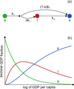
Figure 1: Illustration of the transfer model. (a) The three sectors, agrarian $a$, industrial $i$, and service $s$, are represented by colored circles. The arrows indicate possible transfer paths and their parameters as defined in Eqs. (1)-(3). (b) Typical evolution of sectoral composition as a function of the logarithm of per capita GDP (here: $k_{1}=1$, $k_{2}=0.5$, $\alpha=1$).

An additional parameter, $g_{0}$, emerges from the boundary conditions, i.e. from the value of $g$ where $a=1$, and has the character of a shift along the $g$-axis. Figure 1 illustrates the model and shows schematic trajectories. Parameter $k_{1}$ determines the transfer from the agrarian sector, which, depending on $\alpha$, is split into contributions to the industrial or service sectors. Moreover, $k_{2}$ determines the transfer from industrial to service. E.g. for $k_{1}>0$, $k_{2}>0$, and $\alpha=1$ transfer takes place from $a$ to $i$ and continuously from $i$ to $s$, leading to monotonously decreasing agrarian and increasing service whereas the industrial sector exhibits a maximum (Fig. 1(b)). Except for the trivial case, the model does not have any steady state.

III Results

type	$k_{1}$	$k_{2}$	$\alpha$	transfer	number of
				behavior	countries
1	$>0$	$>0$	$<1$	$a\rightarrow i$, $i\rightarrow s$, $a\rightarrow s$	59
2	$>0$	$>0$	$>1$	$a\rightarrow i$, $i\leftrightarrows s$, $a\text{ -- }s$	25
3	$>0$	$<0$	$<1$	$a\rightarrow i$, $i\leftarrow s$, $a\rightarrow s$	43
4	$>0$	$<0$	$>1$	$a\rightarrow i$, $i\leftarrow s$, $a\text{ -- }s$	0
5	$<0$	$>0$	$<1$	$a\leftarrow i$, $i\rightarrow s$, $a\leftarrow s$	3
6	$<0$	$>0$	$>1$	$a\leftarrow i$, $i\rightarrow s$, $a\text{ -- }s$	1
7	$<0$	$<0$	$<1$	$a\leftarrow i$, $i\leftarrow s$, $a\leftarrow s$	1
8	$<0$	$<0$	$>1$	$a\leftarrow i$, $i\rightleftarrows s$, $a\text{ -- }s$	5

Table 1: Types of sectoral GDP transfer as obtained from the fitting parameters of the model Eqs. (1)-(3). The types are defined according to the sign of the parameters $k_{1}$ and $k_{2}$ as well as if $0<\alpha<1$ or $\alpha>1$. The parameters also specify between which sectors there is a transfer and in which direction. For $\alpha>1$ instead of a transfer from the agriculture to the services sector, a transfer occurs between industry and services, depending on the values of $k_{1}$ and $k_{2}$ (indicated by a —). If $k_{1}$ and $k_{2}$ have opposite signs, the flow is in one direction for all possible values of $a$, $i$, and $s$. If $k_{1}$ and $k_{2}$ are positive, flow may occur from $s$ to $i$ for large $a$, while it is reversed for large $i$ (indicated by $\leftrightarrows$). Vice versa for $k_{1}$ and $k_{2}$ negative. Only types $1$+$2$ have a convergent asymptotic behavior, namely $a\rightarrow 0$, $i\rightarrow 0$, $s\rightarrow 1$ for $g\rightarrow\infty$. Most countries belong to the types 1-3. The remaining types are type 5 (Guinea-Bissau, Madagascar, Vanuatu), type 6 (Ivory Coast), type 7 (Cameroon), and type 8 (Burkina Faso, Morocco, Sudan, Venezuela, South Africa). The special cases $k_{1}=0$, $k_{2}=0$, $\alpha=0$ or $\alpha=1$ did not occur.

We fit the model Eqs. (1)-(3) with a two step procedure, using global country-level data . In the first step, the logarithmic form of Eq. (4), as introduced later, was used to identify $k_{1}$ and an initial value of $g_{0}$ by using a linear regression between $\log(a)$ and $g$. In the second step, $k_{2}$, $\alpha$, and $g_{0}$ were estimated by using the R-implementation of the shuffled complex evolution algorithm (Duan et al., 1993) to minimize the sum of the mean squared errors between $a$, $i$, $s$ from the model and the corresponding observed values. To obtain more reasonable fits, we restricted the parameter ranges as follows: $-5<k_{2}<5$, $0<\alpha<5$, and $1<g_{0}<15$.

For 176 out of 246 countries the available data was sufficient, i.e. data on GDP/cap was available for at least 4 years, and for 137 countries the fitting worked reasonable (we choose $0.1$ as the threshold for the sum of the mean squared error between the data and the fits of all sectors). Due to an anomalous decline of $g$ after dissolution of the Soviet Union, disbandment of the Warsaw Pact, and the breakup of Yugoslavia, respectively, the data before 1995 has been disregarded, in the case of the corresponding countries. For the same reason, data from Liberia and Mongolia prior to 1995 was omitted.

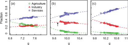
Figure 2: Examples of sectoral GDP fractions versus the logarithm of GDP/cap. (a) Pakistan, (b) Finland, and (c) the United States. Open symbols represent the observed values, solid lines the fitted functions according to Eqs. (1)-(3), and dashed lines extrapolations for illustration. The fitted parameters are (a) Pakistan ($k_{1}=0.56$, $k_{2}=-0.01$, $\alpha=0.32$, $g_{0}=8.12$), (b) Finland ($k_{1}=2.29$, $k_{2}=0.35$, $\alpha=0.50$, $g_{0}=8.74$), and (c) the United States ($k_{1}=1.76$, $k_{2}=0.94$, $\alpha=1.27$, $g_{0}=5.02$). For Finland, the maximum of the industrial sector, $g_{{\rm max}i}\approx 9.7$, is indicated by a black arrow in (b).

Typical examples for which the model results were accepted are depicted in Fig. 2 together with the obtained fits. In all three examples the model agrees reasonably with the data. In the case of Pakistan, the fraction of industry overtakes the fraction of agriculture at $g_{a\times i}\approx 7.5$ ($1,800$ $/cap). The industrial fraction of Finland reached it’s maximum at $g_{{\rm max}i}\approx 9.7$ ($16,300$ $/cap). The service sector is the largest and still increasing for these examples. In the case of the USA, the agrarian sector has a very low contribution.

Different parameter ranges imply different behavior, e.g. $k_{1}<0$ means that the country transfers economic activity to agriculture with increasing GDP/cap. In total there are two different cases for each parameter leading to eight combinations. Table 1 gives an overview of the corresponding types together with the transfer behavior, i.e. economic transfer from which sector to which, and the frequency of each type. Almost half of the considered countries belong to type 1, the traditional path from the agrarian, via industrial, to the service sector. The second most frequent is type 3, which includes a transfer from the service to industrial sector. Another big group consists of type 2 countries, i.e. with transfer from agrarian to industry and flows between industry and services depending on the development. All other types are less populated, type 4 does not occur at all. The occurrence of types 5-8 might be due to noise in the data. Only types 1&2 and 7&8 exhibit a maximum of the industrial sector at $g_{{\rm max}i}=\frac{\log(k_{1}/k_{2})}{k_{1}-k_{2}}+g_{0}$. The examples from Fig. 2 are of type 3 (Pakistan), type 1 (Finland), and type 2 (USA).

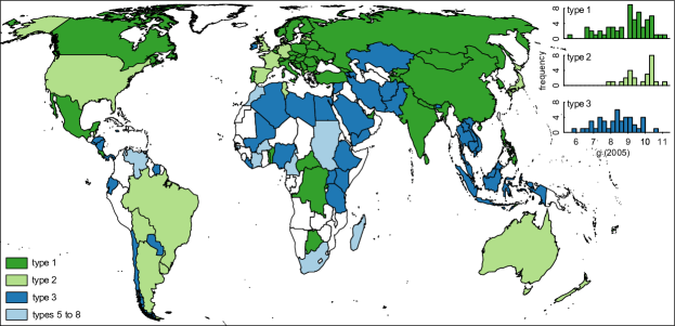
Figure 3: Types of sectoral GDP transfer, geographic location, and frequency. The resolves the three most common types 1-3 (Tab. 1) and the remaining types 5-8. Countries with insufficient data or bad fitting are not colored. Countries of the same type tend to be neighbors. The inset in the upper right corner shows the frequency of countries according to their $g$ (log of GDP/cap) in 2005 for the types 1-3.

On the world map, Fig. 3, one can see which country belongs to which type. Type 1 consists of big parts of Asia and Eastern Europe, some countries in Africa, Canada, and Mexico. The USA, Brazil, other Southern American countries, Western European countries, Japan, and Australia belong to type 2. Type 3 is mainly found in Africa, Middle East, Central Asia, South-East Asia, and a few times in Southern America. A strong regionality can be observed and neighboring countries tend to belong to the same types. It is apparent that most developed countries belong to either type 1 or type 2. At this stage it is not clear what the decisive factor is and further analysis including other economic data could help to pinpoint the most relevant influences of the countries economic paths. Methods from network theory have been applied to analyze the economic productions of countries, indicating that neighboring countries instead of diversifying tend to compete over the same markets Caldarelli et al. (2012).

The inset of Fig. 3 shows the histograms of $g$ (year 2005) for the types 1-3. Type 1 and 3 countries are spread over a wide range of GDP/cap, whereas there is a tendency of type 1 countries to higher GDP/cap ($g>9$) compared to the type 3 case. Type 2 countries generally tend to larger GDP/cap. Surprisingly, many high GDP/cap countries belong to type 2 and not to type 1. Accordingly, their economic growth follows the traditional path $a\rightarrow i\rightarrow s$ but depending on the state of $a$ and $i$, the flow between $i\rightarrow s$ may be increased (high $i$), decreased, or even reversed (high $a$) (see Tab. 1). Type 3, which is the second most frequent one, also follows the traditional path from the agrarian to the industry and service sector, but comes along with a transfer from the service sector to the industry sector, $a\rightarrow i\leftarrow s$, $a\rightarrow s$. This version seems to be characteristic for many developing economies – although not exclusively.

IV Data Collapse

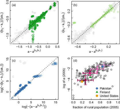
Figure 4: Data collapse according to Eq. (7) and correlations between agrarian sector and rural population. Panels (a)-(c) display the transformed values of all countries and all years. (a) type 1, (b) type 2, and (c) type 3, see Tab. 1. For clarity, in (c) the signs have been changed and the logarithm taken. The underlying grey data points show the values of all other types. The dashed lines have slope $1$ and intercept $0$. For some countries the fitting does not perform well, in particular (a) Singapore (at approx. $-0.8$,$-0.35$) and Bulgaria (approx. between $-0.8$,$-1.2$ and $-0.8$,$-1.8$), (b) Denmark (at approx. $-0.7$,$-0.14$), and (c) Saudi Arabia (at approx. $0.6$,$2.9$) and the Maldives (at approx. $14.6$,$12.9$). Panel (d) shows for the year 2005 $\log a$ versus the fraction of rural population, based on data from the World dataBank. The open circles represent the values of all countries with available data and exhibit a correlation coefficient of $0.69$. The examples from Fig. 2 are highlighted with filled symbols, i.e. Pakistan (diamond), Finland (triangle), and USA (circle). The filled squares with error-bars represent averages and standard deviations of GDP/cap quartiles, i.e. lowest (light, top right) to highest (dark, lower left).

In order to test the universality and applicability of the model, we derive a collapsed representation of all data. We start from solutions of Eqs. (1)-(3)

$$a(g) = {\rm e}^{-k_{1}(g-g_{0})}$$ (4)

$$i(g) = \frac{\alpha k_{1}}{k_{2}-k_{1}}\left({\rm e}^{-k_{1}(g-g_{0})}-{\rm e}^{-k_{2}(g-g_{0})}\right)$$ (5)

$$s(g) = 1-a(g)-i(g)\,.$$ (6)

Eliminating $(g-g_{0})$ in Eq. (4) and (5) one obtains a relation between $a(g)$ and $i(g)$

$$\frac{k_{2}-k_{1}}{\alpha k_{1}}i(g)=\left(a(g)-a(g)^{k_{2}/k_{1}}\right)\,,$$ (7)

allowing to collapse the data of all countries and all years, i.e. independent of $g$. In Fig. 4(a)-(c) we plot the transformed data and separate the three most frequent types for better visibility into panels. The data generally collapses onto the unity diagonal, despite few countries where deviations are partly due to the fact that values before 1995 have been excluded from the fitting (see above) but the values are still displayed for completeness. The collapse suggests universality Stanley (1999); Malmgren et al. (2009) and supports the applicability of the proposed model.

For the set of countries with reasonable fitting, some of the parameters are correlated non-linearly, i.e. $g_{0}$ and $k_{1}$ as well as $k_{2}$ and $\alpha$. Thus, by introducing global parameters, the number of country-specific ones could be reduced. Moreover, $k_{1}$ is weakly correlated with $g$, suggesting that – from the ensemble point of view – Eq. (4) has rather a log-normal shape, which indicates that the system is not ergodic.

We would like to note that since $g$ is the logarithm of the GDP/cap, $a$ decreases as a power-law with the GDP/cap. Studying the asymptotic behavior of the types as defined in Tab. 1, it turns out, that types 1 and 2 converge to $s=1$ for $g\rightarrow\infty$. The model is confined to specific ranges of $g$, e.g. $g\leq g_{0}$ for negative parameter $k_{1}$. Thus, it is important to keep in mind that fitting the model only characterizes the transfer as it is included in the data. This means, the obtained parameters only capture the behavior of the past.

V Discussion

Finally, $\log a$ is plotted versus the fraction of urban population for the year 2005 in Fig. 4(d). The two quantities are correlated with a correlation coefficient of $0.69$. Despite not being completely linear, the correlations are considerable, implying that low agrarian contribution to the economy’s GDP comes along with less rural population. In order to visualize the relation to overall economic output, Figure 4(d) also includes averages and standard deviations of those countries belonging to GDP/cap quartiles, i.e. the quarter of all countries with highest GDP/cap, the second quarter of countries, etc. As one can see, with increasing GDP/cap, rurality and agrarian GDP share decrease. In other words, a high degree of urbanization comes along with economic development or vice versa. This can be related to the finding that per capita socio-economic quantities such as wages, GDP, number of patents applied, and number of educational and research institutions increase by an approximate factor of $1.15$ with increasing city size Bettencourt and West (2010).

However, as Timberlake Timberlake and Kentor (1983) has pointed out, in the case of developing countries an “overurbanization” with fast growing urban populations and excessive employment in the service sector can also hinder economic growth. Not without reason most developing countries in our model belong to type 3, where economic growth is associated with a sectoral transfer from service to industry.

In summary, we propose a system of ordinary differential equations to characterize the development of the sectoral GDP composition. Despite being very simple and involving only 4 country-specific parameters ($g_{0}$ has only the character of shift along $g$), the model fits for the majority of the countries in the world. Relating agrarian and industrial fractions, we collapse the data of all countries and all years onto a straight line. This could be used as an alternative approach to fit the parameters by means of non-linear techniques.

We find that according to the parameter ranges, the countries belong to eight different types. Most countries are found in three of them; the members are distinct in geography and state of economic development. This suggests that countries with low current GDP/cap follow a different path from early developed countries. Our results could indicate a relation between transfer patterns and economic development. Further analysis of additional socio-economic data could shed light on reasons of economic failure or success.

As with any model, our approach is a strong simplification of reality. Also, we assume that parameters are fixed over time and countries follow a given development pathway. This may be justified by cultural, bio-climatic, and structural conditions, which have been consistent over the period of observation. On the other hand, a transition between characteristic pathways is possible. For workforce distribution of 22 countries from the former Soviet Union and Central as well as Eastern Europe, such a transition analysis has been performed using another simple model based on the three-sector hypothesis (Raiser et al., 2004). A similar transition analysis could be an extension of the work presented.

Since it has been found that countries tend to develop goods which are similar to those they currently produce Hidalgo et al. (2007) and that economically successful countries are extremely diversified Tacchella et al. (2012), it could be also of interest, to extend the analysis to the level of products, in order to enable a more detailed analysis. Furthermore, the inclusion of a “quaternary” sector Kenessey (1987); Selstad (1990) in our model might provide additional insights, but sufficient data is not (yet) available. In this context we would also like to note that many developing countries exhibit an informal service sector which is not included in the official figures. Similarly, in developed countries the products can be very complex so that the separation between industrial and service sector might be fuzzy. Accordingly, already the data analyzed in this study is likely to be affected by inaccuracies.

References

- Clark (1940) C. Clark, The Conditions of Economic Progress (Macmillan, London, 1940).
- Fisher (1939) A. G. B. Fisher, Econ. Rec. 15, 24 (1939).
- Fourastie (1949) J. Fourastie, Le Grand Espoir du XXe Siècle (Gallimard, Paris, 1949).
- Krüger (2008) J. J. Krüger, J. Econ. Surv. 22, 330 (2008).
- Raiser et al. (2004) M. Raiser, M. Schaffer, and J. Schuchhardt, Struct. Change Econ. Dynam. 15, 47 (2004).
- Echevarria (1997) C. Echevarria, Int. Econ. Rev. 38, 431 (1997).
- Kongsamut et al. (2001) P. Kongsamut, S. Rebelo, and D. Xie, Rev. Econ. Stud. 68, 869 (2001).
- Timberlake and Kentor (1983) M. Timberlake and J. Kentor, Sociol. Quart. 4, 489 (1983).
- Pandit and Casetti (1989) K. Pandit and E. Casetti, Ann. Ass. Am. Geogr. 79, 329 (1989).
- Duan et al. (1993) Q. Y. Duan, V. K. Gupta, and S. Sorooshian, J. Optimiz. Theory App. 76, 501 (1993).
- Caldarelli et al. (2012) G. Caldarelli, M. Cristelli, A. Gabrielli, L. Pietronero, A. Scala, and A. Tacchella, PLoS ONE 7, e47278 (2012).
- Stanley (1999) H. E. Stanley, Rev. Mod. Phys. 71, S358 (1999).
- Malmgren et al. (2009) R. D. Malmgren, D. B. Stouffer, A. S. L. O. Campanharo, and L. A. N. Amaral, Science 325, 1696 (2009).
- Bettencourt and West (2010) L. Bettencourt and G. West, Nature 467, 912 (2010).
- Hidalgo et al. (2007) C. A. Hidalgo, B. Klinger, A.-L. Barabási, and R. Hausmann, Science 317, 482 (2007).
- Tacchella et al. (2012) A. Tacchella, M. Cristelli, G. Caldarelli, A. Gabrielli, and L. Pietronero, Sci. Rep. 2, srep00723 (2012).
- Kenessey (1987) Z. Kenessey, Rev. Income Wealth 3, 359 (1987).
- Selstad (1990) T. Selstad, Nor. Geogr. Tidsskr. 44, 21 (1990).
- The Worldbank (2012) The Worldbank (2012).