Harmonic mixing in two coupled qubits: quantum synchronization via ac drives

Abstract

Simulating a system of two driven coupled qubits, we show that the time-averaged probability to find one driven qubit in its ground or excited state can be controlled by an ac drive in the second qubit. Moreover, off-diagonal elements of the density matrix responsible for quantum coherence can also be controlled via driving the second qubit, i.e., quantum coherence can be enhanced by appropriate choice of the bi-harmonic signal. Such a dynamic synchronization of two differently driven qubits has an analogy with harmonic mixing of Brownian particles forced by two signals through a substrate. Nevertheless, the quantum synchronization in two qubits occurs due to multiplicative coupling of signals in the qubits rather than via a nonlinear harmonic mixing for a classical nano-particle.

I Introduction

While the desire of building code-cracking quantum computers Bellac ; Zagoskin2011 remains a long standing goal, its pursuit has pushed forward the enormous progress achieved in quantum mesoscopic physics and quantum nanodevices. These efforts have already resulted in the development of a new class of mesoscopic devices Nori-new ; Nori2 ; smirnov ; mi and even new types of materials known as quantum metamaterials metamat ; ost-zag .

Development of such new devices requires a deep understanding of dynamics of single and multi-qubit systems driven both by ac signals (e.g., electromagnetic radiation, or ac voltage and/or currents) and noise. Following this direction of research, several quantum amplifiers have been recently proposed for one omelya1 and two-qubit omelya2 ; omelya3 systems. The idea omelya1 ; omelya2 was to extend the stochastic resonance phenomenon (amplification by certain amount of noise) for one or two ac driven qubits to enhance quantum coherence. Further analogy omelya3 ; rakh ; param between two-qubit system, a Brownian particle driven in periodic substrate and a parametric amplifier has resulted in a proposal to use two coupled qubits as an amplifier of quantum oscillations.

This work was motivated by the analogy between driven Brownian nanoparticles and a system of coupled qubits. It is well-known that an overdamped particle driven by two harmonic ac signals through the substrate can drift in any desirable direction if frequencies of the two drives are commensurate. This effect known as harmonic mixing mix1 ; mix2 ; mix3 ; mix4 ; mix5 ; mix6 ; mix7 ; mix8 ; mix9 has been already observed in many systems, including vortices in superconductors marat , nanoparticles driven through a pore nanopore , current driven Josephson junctions ustinov etc. This suggests an idea that a coupled two-qubit system also should exhibit a harmonic mixing behaviour, but in contrast to the usual classical harmonic mixing for overdamped particles, quantum harmonic mixing should be via parametric coupling of two drives in the quantum master equation. This effect can be used to synchronize quantum oscillations in the two qubits and can control the average probability for a qubit to stay in either ground or excited state by changing the relative phase and/or frequencies of the bi-harmonic drive.

Further, our results can be applied to the case when one needs to control qubits, which do not have their own control circuitry for the reasons of limiting the decoherence brought in by such extra elements, or because of accessibility (e.g., in case of 2D or 3D qubit arrays everitt ; 2djosephson with control circuitry placed at the boundary viz. surface of the device). Similar problems arise in the so-called indirect quantum tomography (see e.g., Ref.fn1, ) or in quantum computations with access to a limited number of qubits (see e.g., Ref. fn2, ). In all these cases, the proposed method of harmonic mixing in qubits allows to control the state of the second (not directly accessible qubit) by varying the frequency and/or phase of the first (accessible) qubit.

II Model

In order to describe a two-qubit system we will use a Hamiltonian in a spin-representation for each qubit with the so called $\sigma_{x}-\sigma_{x}$ coupling:

$$H=-\frac{1}{2}\sum_{j=1,2}\left[\Delta_{j}\;\sigma^{j}_{z}+\epsilon_{j}(t)\;\sigma^{j}_{x}\right]+g\;\sigma^{1}_{x}\>\sigma^{2}_{x}$$ (1)

where $\sigma^{j}_{z}$ and $\sigma^{j}_{x}$ are Pauli matrices corresponding to either the first ($j=1$) or the second ($j=2$) qubit. The tunnelling splitting energies $\Delta_{j}$ are usually determined by the geometry and fabrication details of the specific device, while the bias energies $\epsilon_{j}$ can be driven externally. For simplicity, we consider two identical qubits; that is, we assume $\Delta_{1}=\Delta_{2}=\Delta$. Let us drive the qubits by a controlled bi-harmonic drive:

$$\epsilon_{1}(t)=A_{1}\sin(\omega_{1}t)$$

$$\epsilon_{1}(t)=A_{2}\sin(\omega_{2}t+\phi)$$ (2)

In other words, each qubit is driven by its own signal and amplitudes, frequencies and relative phase of these two signal can be varied at will. The question arises if and under what conditions the second qubit can influence the coherence and occupation of the ground and excited states of the first one. Therefore, we are interested if the second qubit can be used to control the state of the first qubit via dynamic synchronization of their quantum oscillations.

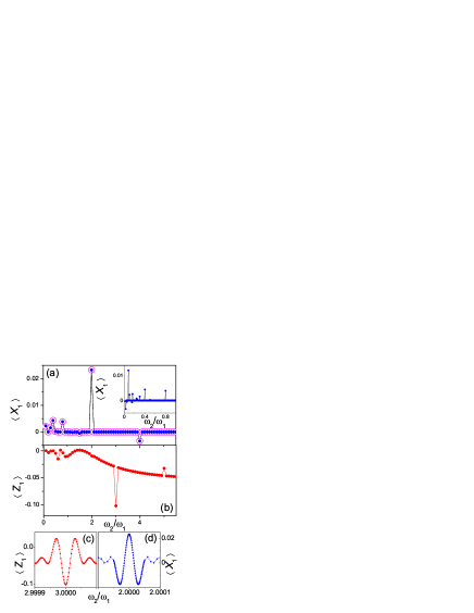
Figure 1: Time-averaged Bloch tensor components $\langle X_{1}\rangle=\langle\Pi_{0x}\rangle$ (a) and $\langle Z_{1}\rangle=\langle\Pi_{0z}\rangle$ (b) for two coupled qubits driven by the two harmonic drives (2) with parameters: $A_{1}=A_{2}=10$, $\phi=0$, $\omega_{1}=2\sqrt{\Delta^{2}+g^{2}}$ and the averaging time interval $5.6\times 10^{4}<\omega_{t}t<1.4\times 10^{5}$ (thus, averaging time $T$ was $8.4\times 10^{4}/\omega_{1}$). Other parameters are the simulation step $dt=1.13\times 10^{-5}$, the number of simulation steps $5\times 10^{9}$, damping $\Gamma=10^{-3}$, coupling constant $g=1$, the tunneling splitting energies $\Delta=1$. To veryfy our numerical results we simulate by using both Euler (open circles) and second-order multidirivative methods (filled circles). The time-averaged Bloch tensor element $\langle X_{1}\rangle$ responsible for the qubit coherence shows peaks at $\omega_{2}/\omega_{1}=2/5,4/5,2,4$, while the time averaged component $\langle Z_{1}\rangle$ peaks at $\omega_{2}/\omega_{1}=3/5,9/10,3,5$. Also, pumping of the excited state for incommensurate frequencies is clearly seen: $|\langle Z_{1}\rangle|$ increases for $\omega_{2}\gtrsim 2\omega_{1}$. By simulating the ten times denser point mesh for frequency ratios from 0.01 to 1 (see inset in (a)) we have obtained extra commensurate resonance frequency ratios but still could not resolve width resonances, which is consistent (see, e.g., Ref. mix8, ) with zero-width harmonic mixing resonances in classical nonlinear devices, where the response near resonances behave as $\cos\Delta\omega T$, where $T$ is the observation time, and $\Delta\Omega$ is detuning. In order to check whether we have a similar behaviour for qubit harmonic mixing, we have simulated $\langle Z_{1}\rangle$ and $\langle X_{1}\rangle$ (panels (c) and (d)) near resonances $\omega_{2}/\omega_{1}=3$ and 2 with frequency detuning $\Delta\omega<1/T$ and observed finite resonance width and oscillations near resonances similar to classical harmonic mixing.

The two-qubit density matrix $\hat{\rho}$ can be written as

$$\hat{\rho}=\frac{1}{4}\sum_{a,b=0,x,y,z}\Pi_{ab}\>\sigma^{1}_{a}\otimes\sigma^{2}_{b}.$$ (3)

This is a straightforward generalization of the standard representation of the single-qubit density matrix expression using the Bloch vector; the components $\Pi_{ab}$ thus constitute what can be called the Bloch tensor. Then, the master equation,

$$\frac{d\hat{\rho}}{dt}=-i\left[\hat{H}(t),\hat{\rho}\right]+\hat{\Gamma}\hat{\rho},$$ (4)

can be written down directly, using the standard approximation for the dissipation operator $\hat{\Gamma}$ via the dephasing $(\Gamma_{\phi 1},\Gamma_{\phi 2})$, and relaxation $(\Gamma_{1},\Gamma_{2})$ rates, to characterize the intrinsic noise in the system. The master equation (3) can be explicitly written as follows omelya2 ; omelya3 :

$$\begin{array}[]{lll}\dot{\Pi}_{0x}&=&\Delta_{2}\Pi_{0y}-\Gamma_{\phi 2}\Pi_{0x}\\ \dot{\Pi}_{0y}&=&-\Delta_{2}\Pi_{0x}+\epsilon_{2}(t)\Pi_{0z}-2g\Pi_{xz}-\Gamma_{\phi 2}\Pi_{0y}\\ \dot{\Pi}_{0z}&=&-\epsilon_{2}(t)\Pi_{0y}+2g\Pi_{xy}-\Gamma_{2}(\Pi_{0z}-Z_{T2})\\ &&\\ \dot{\Pi}_{x0}&=&\Delta_{1}\Pi_{y0}-\Gamma_{\phi 1}\Pi_{x0}\\ \dot{\Pi}_{y0}&=&-\Delta_{1}\Pi_{x0}+\epsilon_{1}(t)\Pi_{z0}-2g\Pi_{zx}-\Gamma_{\phi 1}\Pi_{y0}\\ \dot{\Pi}_{z0}&=&-\epsilon_{1}(t)\Pi_{y0}+2g\Pi_{yx}-\Gamma_{1}(\Pi_{z0}-Z_{T1})\\ &&\\ \dot{\Pi}_{xx}&=&\Delta_{2}\Pi_{xy}+\Delta_{1}\Pi_{yx}-(\Gamma_{\phi 1}+\Gamma_{\phi 2})\Pi_{xx}\\ \dot{\Pi}_{xy}&=&-2g\Pi_{0z}-\Delta_{2}\Pi_{xx}+\Delta_{1}\Pi_{yy}\\ &+&\epsilon_{2}(t)\Pi_{xz}-(\Gamma_{\phi 1}+\Gamma_{\phi 2})\Pi_{xy}\\ \dot{\Pi}_{yx}&=&-2g\Pi_{z0}-\Delta_{1}\Pi_{xx}+\Delta_{2}\Pi_{yy}\\ &+&\epsilon_{1}(t)\Pi_{xz}-(\Gamma_{\phi 1}+\Gamma_{\phi 2})\Pi_{yx}\\ \dot{\Pi}_{xz}&=&2g\Pi_{0y}-\epsilon_{2}(t)\Pi_{xy}+\Delta_{1}\Pi_{yz}-(\Gamma_{\phi 1}+\Gamma_{2})\Pi_{xz}\\ \dot{\Pi}_{zx}&=&2g\Pi_{y0}-\epsilon_{1}(t)\Pi_{yx}+\Delta_{2}\Pi_{zy}-(\Gamma_{\phi 2}+\Gamma_{1})\Pi_{zx}\\ \dot{\Pi}_{yy}&=&-\Delta_{1}\Pi_{xy}-\Delta_{2}\Pi_{yx}\\ &+&\epsilon_{2}(t)\Pi_{yz}+\epsilon_{1}(t)\Pi_{zy}-(\Gamma_{\phi 1}+\Gamma_{\phi 2})\Pi_{yy}\\ \dot{\Pi}_{yz}&=&-\Delta_{1}\Pi_{xz}-\epsilon_{2}(t)\Pi_{yy}\\ &+&\epsilon_{1}(t)\Pi_{zz}-(\Gamma_{\phi 1}+\Gamma_{2})\Pi_{yz}\\ \dot{\Pi}_{zy}&=&-\Delta_{2}\Pi_{zx}-\epsilon_{1}(t)\Pi_{yy}\\ &+&\epsilon_{2}(t)\Pi_{zz}-(\Gamma_{1}+\Gamma_{\phi 2})\Pi_{zy}\\ \dot{\Pi}_{zz}&=&-\epsilon_{1}(t)\Pi_{yz}-\epsilon_{2}(t)\Pi_{zy}\\ &-&(\Gamma_{1}+\Gamma_{2})(\Pi_{zz}-Z_{T1}Z_{T2})\end{array}$$ (28)

Also, for simplicity, hereafter we assume that the relaxation rates are the same for both identical qubits, i.e., $\Gamma_{\phi 1}=\Gamma_{\phi 2}=\Gamma_{\phi}$ and $\Gamma_{1}=\Gamma_{2}=\Gamma_{r}$, and the temperature is low enough, resulting in $Z_{T2}=Z_{T1}=1$, where $Z_{Tj}=\tanh(\Delta_{j}/2k_{B}T_{j})$ is the equilibrium value of the $z$-component of the Bloch vector. This set of ordinary differential equations is an ideal starting point for numerical analysis of the dynamics of two driven and dissipative qubits as it has been proved before omelya2 ; omelya3 . We will simulate these differential equations for two differently driven qubits and will study quantum harmonic mixing.

In the limit of zero coupling, $g=0$, there exists a solution of Eqs. (28) with no entanglement between the qubits. This solution can be written as a direct product of two independent density matrices expressed through their Bloch vectors:

$$\hat{\rho}_{j}=\frac{1}{2}(1+X_{j}\sigma_{x}+Y_{j}\sigma_{y}+Z_{j}\sigma_{z}).$$ (29)

The components of the Bloch tensor $\Pi_{ab}$ are all zero with the exception of

$$(\Pi_{ox},\Pi_{oy},\Pi_{oz})=(X_{1},Y_{1},Z_{1});\>\>(\Pi_{xo},\Pi_{yo},\Pi_{zo})=(X_{2},Y_{2},Z_{2})\;,$$ (30)

which are just the separate qubits’ Bloch vector components. The density matrix components $\Pi_{ox}=X_{1}$, $\Pi_{xo}=X_{2}$, $\Pi_{oy}=Y_{1}$, $\Pi_{yo}=Y_{2}$, $\Pi_{oz}=Z_{1}$, and $\Pi_{zo}=Z_{2}$ can be often directly accessible in experiments. For instance, for two coupled flux qubits the circulating currents in each qubit are proportional to $X_{1}$ or $X_{2}$, respectively (see e.g., Ref. omelya1, ), while $Z_{1}$ and $Z_{2}$ determine the occupation probabilities of the upper (lower) level for the first and the second qubit:

$$P_{\pm,j}=\frac{1}{2}\left(1\mp Z_{j}(t)\right)$$ (31)

with $j=1$ or 2.

III Simulation results

We simulated the set (28) by using the standard Euler method which has been proved to converge well for low-noise drives omelya2 ; omelya3 and analyzed the time-averaged diagonal element of density matrix $\langle X_{1}\rangle=\langle\Pi_{ox}\rangle=\lim_{T\rightarrow\infty}\int_{0}^{T}\Pi_{ox}dt/T$, responsible for the mean coherence in the first qubit, as well as the time-averaged density matrix element $\langle Z_{1}\rangle=\langle\Pi_{oz}\rangle=\lim_{T\rightarrow\infty}\int_{0}^{T}\Pi_{oz}dt/T$, responsible for the mean occupation of the ground and excited states in the first qubit. To verify validity of our numerical results we have also used higher-order multiderivative methods to prove the stability of our numerical procedure (compare the open circles for Euler methods and the filled circles for the second order method in Fig. 1 and 2).

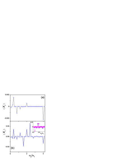
Figure 2: Time-averaged Bloch tensor components $\langle X_{1}\rangle=\langle\Pi_{0x}\rangle$ for two coupled qubits driven by the two harmonic drives (Eq.(2)) with the same parameters as in Fig. 1 and driving frequency $\omega_{1}=\sqrt{\Delta^{2}+g^{2}}-g$ (a) equal to an energy level transition frequency omelya3 and for $\omega_{1}=2.113(\sqrt{\Delta^{2}+g^{2}}-g)$ (b) which is away from the energy level transition. Simulations with a ten-time denser point mesh for frequency ratio from 0.01 to 1 (see inset in (a)) uncovered some extra commensurate frequency ratio where peaks in $\langle X_{1}\rangle$ occurs.

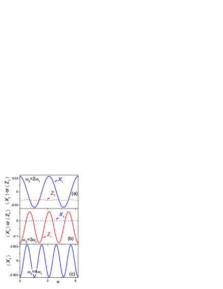
Figure 3: Dependence of $\langle X_{1}\rangle$ and $\langle Z_{1}\rangle$ on the relative phase of two drives of the bi-harmonic signal at different frequency ratio $\omega_{2}/\omega_{1}=2$ (a), 3(b), 4(c). All other parameters are the same as in Fig. 1. For even frequency ratio, where $\langle X_{1}\rangle$ has a peak (Fig.1), the strong dependence of $\langle X_{1}\rangle(\varphi)$ and a week dependence of $\langle Z_{1}\rangle(\varphi)$ occurs, while, for odd ratio of $\omega_{2}/\omega_{1}$, dependence of $\langle Z_{1}\rangle(\varphi)$ is clearly seen and $\langle X_{1}\rangle(\varphi)$ is negligible. The periods of functions $\langle X_{1}\rangle(\varphi)$ and $\langle Z_{1}\rangle(\varphi)$ are controlled by the frequency ratio and are equal to $2\pi\omega_{1}/\omega_{2}$ (for $\omega_{2}>\omega_{1}$).

As we expected, there is no mean coherence $\langle X_{1}\rangle\approx 0$ for most of frequency ratio $\omega_{1}/\omega_{2}$ apart from the specific commensurate cases (e.g., $\omega_{1}/\omega_{2}=2/5,4/5,2,4$, see Fig.1a). Such a situation reminds of a usual classical harmonic mixing for nanoparticles (see, e.g., mix8 ), however, the frequency ratios where peaks occur, are also tuneable by changing the absolute value of signal frequency in either the first or the second qubit. Indeed, choosing the frequency $\omega_{1}$ to be equal to the inter-level spacing frequency $\omega_{1}=\sqrt{\Delta^{2}+g^{2}}-g$ (Fig. 1a) or $\omega_{1}=2\sqrt{\Delta^{2}+g^{2}}$ (Fig.2a) or even away from the inter-level resonances $\omega_{1}=2.113(\sqrt{\Delta^{2}+g^{2}}-g)$ (Fig. 2b) results in a qualitatively similar peak structure, but showing different sequence of the frequency ratios. Indeed, for $\omega_{1}=2.113(\sqrt{\Delta^{2}+g^{2}}-g)$ (Fig. 2b), several new frequency ratios corresponding to the enhancement of qubit coherence occur at $\omega_{2}/\omega_{1}=2/5,4/5,6/5,8/5,2,12/5,14/5,4$. Moreover, some peaks can even change their signs (compare peaks at $\omega_{2}/\omega_{1}=4/5$ in Fig. 1a, 2a, 2b) indicating that both the frequency ratio and the absolute value of frequency can be used to tune qubit harmonic mixing. Such a behaviour is quite unusual with respect to classical harmonic mixing (see e.g., mix3 ) where the frequency ratio is defined by nonlinearity of the system. In contrast, the master equation set (28) is linear and harmonic mixing occurs via a mixture of multiplicative drives as in the qubit parametric oscillator. As we have recently shown, this results in a quite unusual spectra of $\Pi_{a,b}$, and in particular $X_{1}$ and $Z_{1}$ with many harmonic peaks showing complex hierarchy. This can explain a non-trivial behaviour of harmonic mixing changes when varying $\omega_{1}$ or $\omega_{2}$. Note also, that the quantum harmonic mixing occurs in both cases: when (i) $\omega_{1}$ is equal to inter-level spacing and (ii) away from this situation. Therefore, there is no need to tune the parameters of the external drives to any characteristic internal frequency of the two qubit system to observe quantum harmonic mixing.

We have also observed a similar harmonic mixing in time-averaged matrix element $\langle Z_{1}\rangle$ responsible for the occupation of the excited and ground states (Fig. 1b). Interestingly, the peaks in $\langle Z_{1}\rangle$ occur at different ratios of bi-harmonic drive $\omega_{2}/\omega_{1}=3/5,9/10,3,5$. However, such a behaviour is perfectly consistent with the harmonic spectra of $\langle Z_{1}\rangle$ and $\langle X_{1}\rangle$ studied in omelya3 . Indeed, the specrum of $X_{1}$ contains only odd harmonics, while the spectrum of $Z_{1}$ consist of even harmonics in agreement with the fact that peaks of $\langle X_{1}\rangle$ and $\langle Z_{1}\rangle$ have a different parity. Moreover, apart from the peaks at the specific commensurate frequencies, the value of $|\langle Z_{1}\rangle|$ gradually increases with the frequency for $\omega_{2}\gtrsim 2\omega_{1}$ indicating pumping in the excited state even for incommensurate frequencies.

Following the analogy with classical harmonic mixing mix8 , we expect the dependence of $\langle X_{1}\rangle$ and $\langle Z_{1}\rangle$ on the relative phase $\varphi$ of bi-harmonic drive at commensurate frequencies where peaks have been observed. Indeed, we obtained such a dependence $\langle X_{1}\rangle(\varphi)$ and $\langle Z_{1}\rangle(\varphi)$ shown in Fig. 3(a-c) for the same simulation parameters as in Fig. 1 and for frequency ratios $\omega_{2}/\omega_{1}=2$ (a), 3 (b), 4 (c). The well resolved peaks of $\langle X_{1}\rangle$ at even frequency ratios $\omega_{2}/\omega_{1}=2$ and 4 exhibit a strong dependence on relative phase, while very weak peaks of $\langle Z_{1}\rangle$ at these frequency ratios show almost no dependence on $\varphi$. Comparing figures 3(a) and 3(c), we also conclude that periodicity of the $\langle X_{1}\rangle(\varphi)$ changes with increasing frequency ratio following the rule: $\langle X_{1}\rangle(\varphi+2\pi\omega_{1}/\omega_{4})=\langle X_{1}\rangle(\varphi)$. Therefore, the number of full oscillations increases with frequency ratio $\omega_{2}/\omega_{1}$. This dependence of the $\varphi$-periods of $\langle X_{1}\rangle$ and $\langle Z_{1}\rangle$ oscillations on the frequency ratio of the harmonic drives is analogous to the similar dependence of classical harmonic mixing of a Brownian particle driven by bi-harmonic drive on nonlinear substrate mix8 .

IV Conclusions

We have predicted quantum harmonic mixing in a two-qubit system driven by a bi-harmonic drive. It manifests itself in a set of peaks of time-averaged density matrix components responsible for both qubit coherence and occupation of ground and excited states of the qubits. These peaks can be controlled not only by the ratio of frequencies of the two signals but also by tuning frequencies themselves and by relative phase of the two signals. Such a quantum harmonic mixing can be used to manipulate one driven qubit by applying an additional ac signal to the other qubit coupled with the one we have to control. Indeed, setting the frequency of the second qubit to be three times larger than the one of the first qubit and changing the relative phase of signals in these qubits produces oscillations of the density matrix element $Z_{1}$ with amplitude of about 0.1 according to Fig. 3b. Therefore, by changing the driving signal only in the second qubit should allow us to indirectly vary the occupation probabilities of the upper level in the first qubit between 47 and 58 percent (see eq. (31)). A stronger coupling between the qubits should allow an even larger amplitude of the indirect control of the occupation probability. This effect is obviously robust to a reasonably strong decoherence and energy dissipation in the system.

- (1) M. Le Bellac, A Short Introduction to Quantum Information and Quantum Computation (Cambridge University Press, 2006).
- (2) A.M. Zagoskin, Quantum Engineering, Cambridge University Press (2011).
- (3) J.Q. You, F. Nori, Nature 474, 589 (2011).
- (4) I. Buluta, F. Nori, Science 326, 108 (2009).
- (5) A.Yu. Smirnov, S. Savel’ev, L.G. Mourokh, F. Nori, Euro. Phys. Lett. 80, 67008 (2007).
- (6) A.M. Zagoskin, S. Savel’ev, F. Nori, Phys. Rev. Lett. 98, 120503 (2007).
- (7) A.L. Rakhmanov, A.M. Zagoskin, S. Savel’ev, and F. Nori, Phys. Rev. B 77, 144507 (2008).
- (8) O. Astafiev, A. M. Zagoskin, A. A. Abdumalikov, Jr., Y. A. Pashkin, T. Yamamoto, K. Inomata, Y. Nakamura, and J. S. Tsai, Science 327, 840 (2010); A. A. Abdumalikov, O. Astafiev, A. M. Zagoskin, Yu. A. Pashkin, Y. Nakamura, J. S. Tsai, Phys. Rev. Lett. 104, 193601 (2010).
- (9) A.N. Omelyanchouk, S. Savel’ev, A.M. Zagoskin, E. Il’ichev, F. Nori, Phys. Rev. B 80, 212503 (2009)
- (10) S. Savel’ev, A.M. Zagoskin, A.N. Omelyanchouk, F. Nori, Chem. Phys. 375 180 (2010).
- (11) S. Savel’ev, A. M. Zagoskin, A. L. Rakhmanov, A. N. Omelyanchouk, Z. Washington, and Franco Nori Phys. Rev. A 85, 013811 (2012).
- (12) S. Savel’ev, A.L. Rakhmanov, and F. Nori, Phys. Rev. E 72, 056136 (2005); New J. Phys. 7, 82 (2005).
- (13) V. Damgov, Nonlinear and Parametric Phenomena: Theory and Applications in Radiophysical and Mechnical Systems (World Scientific, Singapore, 2001).
- (14) F. Marchesoni, Phys. Lett. A 119, 221 (1986).
- (15) W. Wonneberger, Solid State Commun. 30, 511 (1979).
- (16) I. Goychuk and P. H’́anggi, Europhys. Lett. 43, 503 (1998).
- (17) J. Lehmann, S. Kohler, P. H’́anggi, and A. Nitzan, J. Chem. Phys. 118, 3283 (2003).
- (18) J. Luczka, R. Bartussek, and P. Hänggi, Europhys. Lett. 31, 431 (1995); P. H’́anggi, R. Bartussek, P. Talkner, and J. Luczka, ibid. 35, 315 (1996).
- (19) R. Guantes and S. Miret-Artés, Phys. Rev. E 67, 046212 (2003).
- (20) M. Barbi and M. Salerno, Phys. Rev. E 63, 066212 (2001).
- (21) S. Savel’ev, F. Marchesoni, P. H’́anggi, F. Nori, Phys. Rev. E 70, 066109 (2004); Europhys. Lett. 67, 179 (2004); Eur. Phys. J. B 40, 403 (2004).
- (22) S. Savel’ev, F. Marchesoni, F. Nori, Phys. Rev. Lett. 92, 160602 (2004).
- (23) S. Ooi, S. Savel’ev, M. B. Gaifullin, T. Mochiku, K. Hirata, and F. Nori, Phys. Rev. Lett. 99, 207003 (2007).
- (24) E Kalman, K Healy, Z. S Siwy, Europhysics Letters (EPL) 78, 28002 (2007).
- (25) A. V. Ustinov, C. Coqui, A. Kemp, Y. Zolotaryuk, M. Salerno, Phys. Rev. Lett. 93, 087001 (2004).
- (26) M. J. Everitt, J. H. Samson, S. E. Savel’ev, T. P. Spiller, R. Wilson, A. M. Zagoskin, arXiv:1208.4555 (2012).
- (27) D. Zueco, J. J. Mazo, E. Solano, and J. J. Garcia-Ripoll, Phys. Rev. B 86, 024503 (2012).
- (28) D. Burgarth, K. Maruyama, F. Nori, New J. Phys. 13, 13019 (2011).
- (29) D. Burgarth, K. Maruyama, M.l Murphy, S. Montangero, T. Calarco, F. Nori, M. B. Plenio, Phys. Rev. A 81, 040303(R) (2010).