Classification of global and blow-up
sign-changing solutions of a semilinear heat
equation in the subcritical Fujita range II. Higher-order diffusion

Abstract.

A detailed study of two classes of oscillatory global (and blow-up) solutions was began in [20] for the semilinear heat equation in the subcritical Fujita range

(0.1) $$\textstyle{u_{t}=\Delta u+|u|^{p-1}u\quad\mbox{in}\quad\mathbb{R}^{N}\times\mathbb{R}_{+}\quad\mbox{for}\,\,\,1<p\leq p_{0}=1+\frac{2}{N},}$$

with bounded integrable initial data $u(x,0)=u_{0}(x)$. This study is continued and extended here for the $2m$th-order heat equation, for $m\geq 2$, with non-monotone nonlinearity

(0.2) $$\textstyle{u_{t}=-(-\Delta)^{m}u+|u|^{p}\quad\mbox{in}\quad\mathbb{R}^{N}\times\mathbb{R}_{+},\quad\mbox{in the range}\,\,\,1<p\leq p_{0}=1+\frac{2m}{N},}$$

with the same initial data $u_{0}$. The fourth order bi-harmonic case $m=2$ is studied in greater detail. The blow-up Fujita-type result for (0.2) now reads as follows: blow-up occurs for any initial data $u_{0}$ with positive first Fourier coefficient:

$$\textstyle{\int u_{0}(x)\,{\mathrm{d}}x>0,}$$

i.e., as for (0.1), any such arbitrarily small initial function $u_{0}(x)$ leads to blow-up. The construction of two countable families of global sign changing solutions is performed on the basis of bifurcation/branching analysis and a further analytic-numerical study. In particular, a countable sequence of bifurcation points of similarity solutions is obtained:

$$p_{l}=1+\frac{2m}{N+l},\quad l=0,1,2,...\,.$$

1. Introduction: higher-order semilinear heat equations, blow-up, Fujita exponent, and global oscillatory solutions

This paper generalizes to higher-order (poly-harmonic) diffusion operators the study of [20] of the semilinear second-order heat equation in the subcritical Fujita range

(1.1) $$\textstyle{u_{t}=\Delta u+|u|^{p-1}u\quad\mbox{in}\quad\mathbb{R}^{N}\times\mathbb{R}_{+},\quad\mbox{where}\,\,\,1<p\leq p_{0}=1+\frac{2}{N},}$$

with bounded integrable initial data $u(x,0)=u_{0}(x)$. Necessary key references, results, and our main motivation of the study of (1.1) and further related models can be found in [20, § 1].

1.1. Higher-order semilinear heat equation: blow-up Fujita-like result

Thus, we intend to extend some of key results of [20] to semilinear parabolic equations with higher-order diffusion operators. Such models are steadily becoming more and more popular in various applications and in general PDE theory. Namely, we consider the $2m$th-order heat equation, for $m\geq 2$, in the subcritical Fujita range:

(1.2) $$\textstyle{u_{t}=-(-\Delta)^{m}u+|u|^{p}\quad\mbox{in}\quad\mathbb{R}^{N}\times\mathbb{R}_{+}\quad\mbox{for}\,\,\,1<p\leq p_{0}=1+\frac{2m}{N},}$$

with sufficiently smooth, bounded, and integrable initial data,

(1.3) $$u(x,0)=u_{0}(x)\quad\mbox{in}\quad\mathbb{R}^{N}.$$

The choice of the non-monotone nonlinearity $|u|^{p}$ (a source term) in (1.2) is associated with the necessity of having a standard sounding Fujita-type blow-up result. Namely, it is known [8] that blow-up occurs for (1.2) for any solutions with initial data having positive first Fourier coefficient (see [9] for further details and [21] for an alternative proof):

(1.4) $$\textstyle{\int_{\mathbb{R}^{N}}u_{0}(x)\,{\mathrm{d}}x>0,}$$

i.e., any, even arbitrarily small, such data lead to blow-up. A similar result for positive solutions of (1.1) was well-known since Fujita work in 1966; see [20, § 1] for a survey.

1.2. Results and layout of the paper

In Sections 2–4, we perform construction of countable sets of global sign changing solutions on the basis of bifurcation/branching analysis, as well as of a centre-stable manifold one. Here, we apply spectral theory of related non-self-adjoint $2m$th-order operators [9], which is available for any $m=2,3,...$ . As for (1.1), i.e., for $m=1$, this gives a similar sequence of critical bifurcation exponents:

(1.5) $$p_{l}=1+\frac{2m}{N+l},\quad l=0,1,2,...\,.$$

References and some results for analogous global similarity solutions of a different higher-order reaction-diffusion PDE with a standard monotone nonlinearity as in (1.1),

(1.6) $$u_{t}=-(-\Delta)^{m}u+|u|^{p-1}u\quad(m\geq 2)$$

can be found in [17]. It is remarkable (and rather surprising for us) that the bifurcation-branching phenomena therein for (1.6) are entirely different from those for the present equation (1.2), which turn out also to be more complicated, with various standard and non-standard bifurcation phenomena.

It is worth mentioning here that our study also directly concerns blow-up solutions of (1.1): we claim that, under the conditions that our two classes of its global oscillatory solutions are evolutionary complete (see [20, § 7] for a precise statement and some results for (1.1)), all other solutions of (1.2) must blow-up in finite time. Then this describes a much wider class of blow-up solutions, and actually says that almost all  (with a.a. defined in a natural way) solutions of (1.2) in the subcritical Fujita range blow-up in finite time.

2. Global similarity solutions and $p$-bifurcation branches

In what follows, we use a general scheme and “ideology” of the study in [20] of the second-order semilinear equation (1.1). Therefore, omitting some obvious details, we now more briefly start to describe which results on global solutions can be extended to the $2m$th-order reaction-diffusion equation (1.2) in the subcritical range.

2.1. First family of global patterns: similarity solutions

As usual, for the higher-order model (1.2) with $m\geq 2$, we first study the existence and multiplicity of the standard global (i.e., well defined for all $t>0$) similarity solutions of the form

(2.1) $$u_{S}(x,t)=t^{-\frac{1}{p-1}}f(y),\quad y=x/t^{\frac{1}{2m}}.$$

This leads to the semilinear elliptic problem for the rescaled similarity profile $f$:

(2.2) $$\left\{\begin{matrix}{\bf B}_{1}f+|f|^{p}\equiv-(-\Delta)^{m}f+\textstyle{\frac{1}{2m}}\,y\cdot\nabla f+\textstyle{\frac{1}{p-1}}\,f+|f|^{p}=0\quad\mbox{in}\quad\mathbb{R}^{N},\vskip 3.0pt plus 1.0pt minus 1.0pt\vskip 3.0pt plus 1.0pt minus 1.0pt\\ f(y)\,\,\,\mbox{decays exponentially fast as}\,\,\,|y|\to\infty.\qquad\qquad\qquad\qquad\quad\,\,\end{matrix}\right.$$

For $m=1$, this problem admits a variational setting in a weighted metric of $L^{2}_{\rho}(\mathbb{R}^{N})$, where $\rho={\mathrm{e}}^{|y|^{2}/4}$. This positive fact was heavily used in [20], where category/fibering techniques allowed us to detect a countable number of solutions and bifurcation branches.

However, for any $m\geq 2$, (2.2) is not variational in any weighted $L^{2}$ space; cf. reasons for that and a similar negative result in [23, § 7]. So, those power tools of potential operator theory in principle cannot be applied for (2.2), with any $m\geq 2$.

Moreover, unlike the previous study of (1.1) in [20], we cannot use standard variational results on bifurcation from eigenvalues of arbitrary multiplicity (for our purposes, the results for odd multiplicity [7, p. 381, 401] concerning local and global continuation of branches are sufficient). We also do not have global multiplicity results via Lusternik–Schnirel’man (L–S, for short) and fibering theory. As usual, higher-order semilinear elliptic equations such as (2.2), or even the corresponding ODEs for radially symmetric profiles $f$, become principally different and more difficult than their second-order variational counterparts. We again refer to [2, § 6.7C] for general results on bifurcation diagrams, and to [1, 29] for more detailed results for related $2m$th-order ODEs in 1D. These results do not apply directly but can be used for a better understanding of global bifurcation diagrams of similarity patterns $f(y)$.

Thus, as in [17] for a quite similar looking equation (1.6), for global continuation of branches, we have to rely more heavily on numerical methods, and this is an unavoidable feature of such a study of nonlinear higher-order equations. Surprisingly, we detect completely different local and global properties of $p$-branches in contrast with those in [17] for the equation (1.6), which therefore are not so definitely attached to variational, monotone, or order-preserving (i.e., via the Maximum Principle) features of these difficult global similarity problems studied since the 1980s.

2.2. Fundamental solution and Hermitian spectral theory

We begin with the necessary fundamental solution $b(x,t)$ of the corresponding linear parabolic (poly-harmonic) equation

(2.3) $$u_{t}=-(-\Delta)^{m}u\quad\mbox{in}\quad\mathbb{R}^{N}\times\mathbb{R}_{+},$$

which takes the standard similarity form

(2.4) $$b(x,t)=t^{-\frac{N}{2m}}F(y),\quad\mbox{where}\quad y=x/t^{\frac{1}{2m}}.$$

The rescaled kernel $F$ is then the unique radial solution of the elliptic equation

(2.5) $${\bf B}F\equiv-(-\Delta)^{m}F+\textstyle{\frac{1}{2m}}\,y\cdot\nabla F+\textstyle{\frac{N}{2m}}\,F=0\,\,\,\,{\rm in}\,\,\mathbb{R}^{N},\quad\mbox{with}\,\,\,\textstyle{\int F=1.}$$

The rescaled kernel $F(|y|)$ is oscillatory as $|y|\to\infty$ and satisfies the estimate [10, 14]

(2.6) $$|F(y)|<D\,\,{\mathrm{e}}^{-d|y|^{\alpha}}\,\,\,{\rm in}\,\,\,\mathbb{R}^{N},\quad\mbox{where}\,\,\,\alpha=\textstyle{\frac{2m}{2m-1}}\in(1,2),$$

for some positive constants $D$ and $d$ depending on $m$ and $N$. The linear operator ${\bf B}_{1}$ in equation (2.2) is connected with the operator (2.5) for the rescaled kernel $F$ in (2.4) by

(2.7) $$\textstyle{{\bf B}_{1}={\bf B}+c_{1}I,\quad\mbox{where}\,\,\,c_{1}=\frac{1}{p-1}-\frac{N}{2m}\equiv\textstyle{\frac{N(p_{0}-p)}{2m(p-1)}}\quad\mbox{and}\quad p_{0}=1+\frac{2m}{N}.}$$

In view of (2.7), in order to study the similarity solutions, we need the spectral properties of ${\bf B}$ and of the corresponding adjoint operator ${\bf B}^{*}$. Both are considered in weighted $L^{2}$-spaces with the weight functions induced by the exponential estimate of the rescaled kernel (2.6). For $m\geq 2$, we consider ${\bf B}$ in the weighted space $L^{2}_{\rho}(\mathbb{R}^{N})$ with the exponentially growing weight function

(2.8) $$\rho(y)={\mathrm{e}}^{a|y|^{\alpha}}>0\quad{\rm in}\,\,\,\mathbb{R}^{N},$$

where $a\in(0,2d)$ is any fixed constant and $d$ is as in (2.6). We ascribe to ${\bf B}$ the domain $H^{2m}_{\rho}(\mathbb{R}^{N})$ being a Hilbert space with the norm

$$\textstyle{\|v\|^{2}=\int\rho(y)\sum\limits_{k=0}^{2m}|D^{k}v(y)|^{2}\,\mathrm{d}y,}$$

induced by the corresponding inner product. Then $H^{2m}_{\rho}\subset L^{2}_{\rho}\subset L^{2}$. The spectral properties ${\bf B}$ are as follows [9]:

Lemma 2.1.

(i) ${\mathbf{B}}:H^{2m}_{\rho}\to L^{2}_{\rho}$ is a bounded linear operator with the real point spectrum

(2.9) $$\sigma({\mathbf{B}})=\{\lambda_{l}=-\textstyle{\frac{l}{2m}},\,\,l=0,1,2,...\}.$$

The eigenvalues $\lambda_{l}$ have finite multiplicities with eigenfunctions

(2.10) $$\psi_{\beta}(y)=\textstyle{\frac{(-1)^{|\beta|}}{\sqrt{\beta!}}}\,D^{\beta}F(y),\quad\mbox{for any}\,\,\,|\beta|=l.$$

(ii) The set $\Phi=\{\psi_{\beta}\}_{|\beta|\geq 0}$ is complete and the resolvent $({\mathbf{B}}-\lambda I)^{-1}$ is compact in $L^{2}_{\rho}$.

By Lemma 2.1, the centre and stable subspaces of ${\bf B}$ are given by $E^{c}={\rm Span}\{\psi_{0}=F\}$ and $E^{s}={\rm Span}\{\psi_{\beta},\,|\beta|>0\}$.

Consider next the adjoint (in the dual $L^{2}$-metric) operator

(2.11) $${\bf B}^{*}=-(-\Delta)^{m}-\textstyle{\frac{1}{2m}}\,y\cdot\nabla\,.$$

For $m\geq 2$, we treat ${\bf B}^{*}$ in $L^{2}_{\rho^{*}}$ with the exponentially decaying weight function

(2.12) $$\textstyle{\rho^{*}(y)=\frac{1}{\rho(y)}\equiv{\mathrm{e}}^{-a|y|^{\alpha}}>0.}$$

Lemma 2.2.

(i) ${\bf B}^{*}:H^{2m}_{\rho^{*}}\to L^{2}_{\rho^{*}}$ is a bounded linear operator with the same spectrum $(\ref{spec1})$ as ${\bf B}$. Eigenfunctions $\psi_{\beta}^{*}(y)$ with $|\beta|=l$ are $l$th-order generalized Hermite polynomials given by

(2.13) $$\psi_{\beta}^{*}(y)=\textstyle{\frac{1}{\sqrt{\beta!}}\,\Big{[}y^{\beta}+\sum\limits_{j=1}^{[|\beta|/2m]}\frac{1}{j!}(-\Delta)^{mj}y^{\beta}\Big{]}.}$$

(ii) The set $\Phi^{*}=\{\psi_{\beta}^{*}\}_{|\beta|\geq 0}$ is complete and resolvent $({\mathbf{B}}^{*}-\lambda I)^{-1}$ compact in $L^{2}_{\rho^{*}}$.

It follows that the orthonormality condition holds

(2.14) $$\langle\psi_{\beta},\psi_{\gamma}^{*}\rangle=\delta_{\beta\gamma},$$

where $\langle\cdot,\cdot\rangle$ denotes the standard $L^{2}(\mathbb{R}^{N})$ inner product and $\delta_{\beta\gamma}$ is Kronecker’s delta.

Using (2.14), we introduce the subspaces of eigenfunction expansions and begin with the operator ${\bf B}$. We denote by $\tilde{L}^{2}_{\rho}$ the subspace of eigenfunction expansions $v=\sum c_{\beta}\psi_{\beta}$ with coefficients $c_{\beta}=\langle v,\psi^{*}\rangle$ defined as the closure of the finite sums $\{\sum_{|\beta|\leq M}c_{\beta}\psi_{\beta}\}$ in the norm of $L^{2}_{\rho}$. Similarly, for the adjoint operator ${\bf B}^{*}$, we define the subspace $\tilde{L}^{2}_{\rho^{*}}\subseteq L^{2}_{\rho^{*}}$. Note that since the operators are not self-adjoint and the eigenfunction subsets are not orthonormal, in general, these subspaces can be different from $L^{2}_{\rho}$ and $L^{2}_{\rho^{*}}$, and the equality is guaranteed in the self-adjoint case $m=1$, $a=\frac{1}{4}$ only.

2.3. Existence of similarity profiles close to transcritical bifurcations

Consider the elliptic problem (2.2). Using the above Hermitian spectral analysis of the operator pair $\{{\bf B},{\bf B}^{*}\}$, we formulate the bifurcation problems, which guarantee the existence of a similarity solution in a neighbourhood of bifurcation points. In fact, our consideration is quite similar to that for the second-order case in [20], so we may omit some details. Since $p<p_{0}$, our analysis is performed in the subcritical Sobolev range:

(2.15) $$1<p<p_{S}=\frac{N+2m}{N-2m}\quad\Longrightarrow\quad H^{m}_{\rho}(\mathbb{R}^{N})\subset L^{p+1}_{\rho}(\mathbb{R}^{N})\,\,\,\mbox{compactly}.$$

Taking $p$ close to the critical values, as defined in (1.5), we look for small solutions of (2.2). At $p=p_{l}$, the linear operator ${\bf B}_{1}$ has a nontrivial kernel, hence:

Proposition 2.1.

Let for an $l\geq 0$, the eigenvalue $\lambda_{l}=-\frac{l}{2m}$ of operator $(\ref{ODEf})$ is of odd multiplicity. Then the critical exponent $(\ref{h2})$ is a bifurcation point for the problem $(\ref{1.7R})$.

Proof. Consider in $L^{2}_{\rho}$ our equation written as

(2.16) $$\hat{{\bf B}}f=-(1+c_{1})f-|f|^{p},\quad\mbox{where}\,\,\,\hat{{\bf B}}={\bf B}_{1}-(1+c_{1})I\equiv{\bf B}-I.$$

It follows that the spectrum $\sigma(\hat{{\bf B}})=\{-1-\frac{l}{2m}\}$ consists of strictly negative eigenvalues. The inverse operator $\hat{{\bf B}}^{-1}$ is known to be compact, [9, Prop. 2.4]. Therefore, in the corresponding integral equation

(2.17) $$f=\hat{\bf A}(f)\equiv-(1+c_{1})\hat{{\bf B}}^{-1}f-\hat{{\bf B}}^{-1}(|f|^{p}),$$

the right-hand side is a compact Hammerstein operator; see [26, Ch. V] and applications in [3, 17, 23]. In view of the known spectral properties of $\hat{\bf B}^{-1}$, bifurcations in the problem (2.17) occur if the derivative $\hat{\bf A}^{\prime}(0)=-(1+c_{1})\hat{{\bf B}}^{-1}$ has the eigenvalue $1$ of odd multiplicity, [27, 26]. Since $\sigma(\hat{\bf A}^{\prime}(0))=\{(1+c_{1})/(1+\frac{l}{2m})\}$, we obtain the critical values (1.5). By construction, the solutions of (2.17) for $p\approx p_{l}$ are small in $L^{2}_{\rho}$ and, as can be seen from the properties of the inverse operator, $f$ is small in the domain $H^{2m}_{\rho}$ of ${\bf B}$. Since the weight (2.8) is a monotone growing function as $|y|\to\infty$, using the known asymptotic properties of solutions of (2.2), $f\in H^{2m}_{\rho}$ is a uniformly bounded, continuous function (for $N<2m$, this directly follows from Sobolev’s embedding theorem). ∎

Thus, $l=0$ is always a bifurcation point since $\lambda_{0}=0$ is simple. In general, for $l=1,2,...$ the odd multiplicity occurs depending on the dimension $N$. For instance, for $l=1$, the multiplicity is $N$, and, for $l=2$, it is $\frac{N(N+1)}{2}$. In the case of even multiplicity of $\lambda_{l}$, an extra analysis is necessary to guarantee that a bifurcation occurs [27] using the rotation $\gamma_{l}$ of the vector field corresponding to the nonlinear term in (2.17) on the unit sphere in the eigenspace $\Phi_{l}={\rm Span}\{\psi_{\beta},\,|\beta|=l\}$ (if $\gamma_{l}\not=1$, then bifurcation occurs). We do not perform this study here and note that the non-degeneracy of this vector field is not straightforward; see related comments below. It is crucial that, for main applications, for $N=1$ and for the radial setting in $\mathbb{R}^{N}$, the eigenvalues (2.9) are simple and (1.5) are always bifurcation points. Unlike Proposition 3.2 for $m=1$ [20, § 3], we have the following result describing the local behaviour of bifurcation branches occurring in the main applications, see [26] and [27, Ch. 8]. Unlike the case $m=1$, some bifurcations become transcritical.

Proposition 2.2.

Let $\lambda_{l}$ be a simple eigenvalue of ${\bf B}$ with eigenfunction $\psi_{l}$, and let

(2.18) $$\kappa_{l}=\langle|\psi_{l}|^{p},\psi_{l}^{*}\rangle\not=0.$$

Then the $p$-bifurcation branch crosses transversely the $p$-axis at $p=p_{l}$.

We next describe the behaviour of solutions for $p\approx p_{l}$ and apply the classical Lyapunov–Schmidt method, [27, Ch. 8], to equation (2.17) with the operator $\hat{\bf A}$ that is differentiable at $0$. Since, under the assumptions of Proposition 2.2, the kernel $E_{0}={\rm ker\,}\hat{\bf A}^{\prime}(0)={\rm Span\,}\{\psi_{l}\}$ is one-dimensional, denoting by $E_{1}$ the complementary (orthogonal to $\psi_{l}^{*}$) invariant subspace, we set

(2.19) $$\textstyle{f=F_{0}+F_{1},\quad\mbox{where}\quad F_{0}=\varepsilon_{l}\psi_{l}\in E_{0}\quad\mbox{and}\quad F_{1}=\sum_{k\not=l}\varepsilon_{k}\psi_{k}\in E_{1}.}$$

Let $P_{0}$ and $P_{1}$, $P_{0}+P_{1}=I$, be projections onto $E_{0}$ and $E_{1}$ respectively. Projecting (2.17) onto $E_{0}$ yields

(2.20) $$\gamma_{l}\varepsilon_{l}=-\langle\hat{\bf B}^{-1}(|f|^{p}),\psi_{l}^{*}\rangle,\quad\gamma_{l}=1-\textstyle{\frac{1+c_{1}}{1+l/2m}}=\textstyle{\frac{(N+l)s}{(p-1)(2m+l)}},\quad s=p-p_{l}.$$

By bifurcation theory (see [27, p. 355] or [7, p. 383], where $\hat{\bf A}^{\prime}(0)$ is Fredholm of index zero), $F_{1}=o(\varepsilon_{l})$ as $\varepsilon_{l}\to 0$, so that $\varepsilon_{l}$ is calculated from (2.20) as:

(2.21) $$\textstyle{\gamma_{l}\varepsilon_{l}=-|\varepsilon_{l}|^{p}\langle\hat{\bf B}^{-1}|\psi_{l}|^{p},\psi_{l}^{*}\rangle+o(\varepsilon_{l}^{p})\,\,\Longrightarrow\,\,|\varepsilon_{l}|^{p-2}\varepsilon_{l}=\hat{c}_{l}(p-p_{l})[1+o(1)],}$$

where $\hat{c}_{l}=\textstyle{\frac{(N+l)^{2}}{4m^{2}\kappa_{l}}}$. We have used the following calculation:

$$\textstyle{\langle\hat{\bf B}^{-1}|\psi_{l}|^{p},\psi_{l}^{*}\rangle=\langle|\psi_{l}|^{p},(\hat{\bf B}^{*})^{-1}\psi_{l}^{*}\rangle=-\frac{\kappa_{l}}{1+\frac{l}{2m}}.}$$

Recall the identity $(\hat{\bf B}^{-1})^{*}=(\hat{\bf B}^{*})^{-1}$.

It follows from the algebraic equation in (2.21) that the bifurcations are transcritical provided that $\kappa_{l}\not=0$, while the sign of $\kappa_{l}$ determines how the branches cross the $p$-axis. For $l=0$, it is easy to see that $\kappa_{0}>0$, since $\psi_{0}=F$ and $\psi_{0}^{*}=1$, so that

(2.22) $$\kappa_{0}=\langle|\psi_{0}|^{p},\psi_{0}^{*}\rangle=\int|F|^{p}>0\quad(p=p_{0}).$$

Moreover, for $p_{0}\approx 1^{+}$, by the definition of $F$ in (2.5), we have that $\kappa_{0}\approx 1$. The positivity or negativity of the scalar product (2.18) for $l\geq 1$ and arbitrary $p>1$ is not straightforward, and we should rely on a delicate numerical evidence; see [17]. It turns out that $\kappa_{l}$ can be both positive and negative for different $l\geq 1$.

Let us note the following principal difference in comparison with the case of monotone nonlinearity $+|f|^{p-1}f$ studied before for $m=1$, [20]. It turns out that

(2.23) $$\kappa_{l}=0\quad\mbox{for odd $l=1,3,5,...$},$$

since in (2.18), $|\psi_{l}(y)|^{p}$ is even, while the polynomial $\psi_{l}^{*}(y)$ is odd. This means the following:

(2.24) $$p=p_{l}\quad\mbox{for odd $l\geq 1$ are not {\bf``standard"} bifurcation points.}$$

The corresponding “non-standard” bifurcation phenomenon will be discussed shortly. On the other hand, for the standard monotone nonlinearity as in (1.6), all critical exponents $\{p_{l}\}$ are pitchfork bifurcations, [17].

Thus, under the assumption $\kappa_{l}\not=0$ on the coefficients (2.18), we obtain a countable sequence of bifurcation points (1.5) satisfying $p_{l}\to 1^{+}$ as $l\to\infty$, with typical transcritical bifurcation branches appearing in a neighbourhood. The behaviour of solutions in $H^{2m}_{\rho}$ and uniformly in $\mathbb{R}^{N}$, for $p<p_{S}$, takes the form

(2.25) $$f_{l}(y)=|\hat{c}_{l}(p-p_{l})|^{\frac{1}{p-1}}\,{\rm sign}\,(\hat{c}_{l}(p-p_{l}))\,(\psi_{l}(y)+o(1))\quad\mbox{as}\,\,\,p\to p_{l}.$$

Instability of all these local branches of similarity profiles is studied similar to the case $m=1$ in [20, § 2]; see also [17].

2.4. Lyapunov–Schmidt branching equation in the general multiple case: non-radial patterns

Let now $\lambda_{l}=-\frac{l}{2m}$ have multiplicity $M=M(l)>1$ given by the binomial coefficient

(2.26) $$\textstyle{M(l)={\rm dim}\,W^{c}({\bf B}-\lambda_{l}I)=C_{N+l-1}^{l}=\frac{(N+l-1)!}{l!(N-1)!},\quad\mbox{so that}}$$

(2.27) $$E_{0}={\rm ker}({\bf B}-\lambda_{l}I)={\rm Span}\{\psi_{l1},...,\psi_{lM}\}.$$

Then, looking for a solution

(2.28) $$f=f_{0}+f_{1},\quad\mbox{with}\quad f_{0}=\varepsilon_{1}\psi_{l1}+...+\varepsilon_{M}\psi_{lM},\quad\mbox{where}\quad f_{1}\bot E_{0},$$

and substituting into the equation (2.17), multiplying by $\psi_{li}^{*}$, and denoting, as usual, $s=p-p_{l}$, $0<|s|\ll 1$, we obtain the following generating system of $M$ algebraic equations:

(2.29) $$\varepsilon_{i}=\frac{2m}{s(N+l)^{2}}\,\int|\varepsilon_{1}\psi_{l1}+...+\varepsilon_{M}\psi_{lM}|^{p}\,\psi_{li}^{*}\equiv D_{i}(\varepsilon_{1},...,\varepsilon_{M}),\quad i=1,2,...,M.$$

Here $p=p_{l}$. Denoting $x=(\varepsilon_{1},...,\varepsilon_{M})^{T}\in\mathbb{R}^{M}$, the system (2.29) is written as a fixed point problem for the given nonlinear operator ${\bf D}=(D_{1}(x),...,D_{M}(x))^{T}$,

(2.30) $$x={\bf D}(x)\quad\mbox{in}\quad\mathbb{R}^{M}.$$

In the second-order case $m=1$ [20, § 3], the system (2.30) was variational, that allowed us to get a multiplicity result. In view of the dual metric in (2.14), for any $m\geq 2$, the algebraic system (2.29) is not variational, so the multiplicity of admissible solutions remains an open problem.

Global extension of the above local $p$-bifurcation branches is performed by classic theory of nonlinear compact operators, [7, 26, 27]. However, since the problem is not variational, nothing prevents existence of closed $p$ sub-branches or appearances of turning, saddle-node bifurcations (we will show that this can actually happens), so that the total number and structure of solutions for any $p\in(1,p_{0}]$ remain a difficult problem. We will then inevitably should rely on careful numerics.

2.5. “Non-standard” pitchfork bifurcations for $\kappa_{l}=0$

Without loss of generality, we consider the simplest case $l=1$, $N=1$, $m=2$ (then $p_{1}=1+m=3$ by (1.5)), where, from (2.18) and (2.10), (2.13), it is clear that $\kappa_{1}$ vanishes:

(2.31) $$\textstyle{\kappa_{1}=\langle|\psi_{1}|^{p_{1}},\psi_{1}^{*}\rangle\equiv\int_{\mathbb{R}}\big{|}F^{\prime}(y)|^{3}y\,{\mathrm{d}}y=0.}$$

Next, unlike the standard approximation (2.19) close to $p=3$, we now use an improved one given by the expansion on the 2D invariant subspace $E_{12}={\rm Span}\{\psi_{1},\psi_{2}\}$ (this choice will be explained below):

(2.32) $$f=F_{12}+F_{3},\quad\mbox{where}\quad F_{12}=\varepsilon_{1}\psi_{1}+\varepsilon_{2}\psi_{2}\quad\mbox{and}\quad F_{3}\bot E_{12},$$

with the scalar parameters $\varepsilon_{1}$, $\varepsilon_{2}$ to be determined. For simplicity, we next use the differential version of the integral equation (2.17) for $l=1$:

(2.33) $$\textstyle{({\bf B}-\lambda_{1}I)f-\frac{s}{4}\,f=|f|^{p}+...,\quad\mbox{where}\quad s=p-p_{1}}$$

and where we omit the $O(s^{2})$-term. Substituting (2.32) into (2.33) and projecting onto corresponding one-dimensional subspaces, quite similar to the system (2.29), we obtain the following asymptotic system of two algebraic equations:

(2.34) $$\left\{\begin{matrix}-\frac{s}{4}\,\varepsilon_{1}=-\int|\varepsilon_{1}\psi_{1}+\varepsilon_{2}\psi_{2}|^{3}\psi_{1}^{*}+...,\quad\,\,\,\vskip 3.0pt plus 1.0pt minus 1.0pt\vskip 3.0pt plus 1.0pt minus 1.0pt\\ -\frac{1}{4}\,\varepsilon_{2}=\frac{s}{4}\,\varepsilon_{2}-\int|\varepsilon_{1}\psi_{1}+\varepsilon_{2}\psi_{2}|^{3}\psi_{2}^{*}+...\,,\end{matrix}\right.$$

where we put $\lambda_{2}=-\frac{l}{2m}=-\frac{1}{2}$ (for $l=m=2$) and where we have omitted higher-order terms associated with the orthogonal $F_{3}$ in (2.32) and via replacing $p$ by $p_{1}=3$ in the integrals on the right-hand sides. Then, the second equation, as $s\to 0$, gives the dependence of $\varepsilon_{2}$ on the leading expansion coefficient $\varepsilon_{1}$ on $E_{12}$:

(2.35) $$\textstyle{\varepsilon_{2}=2|\varepsilon_{1}|^{3}\mu_{12}+...,\quad\mbox{where}\quad\mu_{12}=\int|\psi_{1}|^{3}\psi_{2}^{*}\neq 0\quad\mbox{and}\quad\psi_{2}^{*}=\frac{1}{\sqrt{2}}\,y^{2}.}$$

It is crucial that, unlike in (2.31), the coefficient $\mu_{12}$ is given by the integral of some even function, so that, now, the assumption $\mu_{12}\neq 0$ is not that restrictive and can be quite reliably checked numerically.

Next, the first equation in (2.34), after a Taylor expansion in the integral, by using that $\varepsilon_{2}=o(\varepsilon_{1})$ as $s\to 0$, provides us with the necessary bifurcation scalar equation on $\varepsilon_{1}$,

(2.36) $$\textstyle{\frac{s}{4}\,\varepsilon_{1}=\int|\varepsilon_{1}\psi_{1}|^{3}\psi_{1}^{*}+3\varepsilon_{1}^{2}\,{\rm sign}\,\varepsilon_{1}\varepsilon_{2}\nu_{12}+...,\,\,\mbox{with}\,\,\nu_{12}=\int\psi_{1}^{2}({\rm sign}\,\psi_{1})\,\psi_{2}\psi_{1}^{*}\neq 0,}$$

where, again, in $\nu_{12}$, we face an even function in the integral. Since the first coefficient vanishes by (2.23) for $l=1$, $\int|\psi_{1}|^{3}\psi_{1}^{*}=0$, using the dependence (2.35), we obtain

(2.37) $$\textstyle{|\varepsilon_{1}|^{5}=\hat{c}_{12}\,s+...,\quad\mbox{where}\quad\hat{c}_{12}=\frac{1}{24\mu_{12}\nu_{12}}.}$$

It follows that we thus deal with a pitchfork bifurcation at $p=p_{1}=3$, which is subcritical if $\hat{c}_{12}<0$ and supercritical if $\hat{c}_{12}>0$.

Overall, the bifurcation branches take the following form: for, e.g., $\hat{c}_{12}>0$,

(2.38) $$\textstyle{f(y)=\pm[\hat{c}_{12}(p-3)]^{\frac{1}{5}}\psi_{1}(y)+2\mu_{12}[\hat{c}_{12}(p-3)]^{\frac{3}{5}}\psi_{2}(y)+...\quad\mbox{as}\quad p\to 3^{+}.}$$

We will reveal this kind of bifurcation numerically in Section 4. Note that this non-standard bifurcation branch near $p=3$ is more “steep”, $\sim O((p-3)^{\frac{1}{5}}))$, than the standard one in (2.25), which, for $l=1$, is of the order $\sim O(\sqrt{p-3})$.

One can see that a similar bifurcation scenario, under the vanishing assumption (2.23), can be developed by using other invariant subspaces rather than that in (2.32). The crucial conditions then remain the same: the corresponding coefficients $\mu_{..}$ in (2.35) and $\nu_{..}$ in (2.36) must be non-zero, which is possible by mixing even and odd eigenfunctions in the subspace, depending on the multiindices chosen. This has an interesting and surprising consequence:

(2.39) (2.23): there can be more than one bifurcation branch, even for 1D eigenspace.

In Section 4, we will observe this numerically for the one-dimensional eigenspace.

2.6. Transversality of intersections of subspaces

This was a permanent subject of an intense study for nonlinear second-order parabolic equations; see related key references and further comments in [20, § 6.2]. We briefly recall these important results below. Namely, this problem was completely solved rather recently for a scalar reaction-diffusion equation on a circle of the form

(2.40) $$u_{t}={\bf A}(u)\equiv u_{xx}+g(x,u,u_{x}),\quad x\in S^{1}=\mathbb{R}/2\pi{\mathbb{Z}},$$

where the nonlinearity $g(\cdot)$ satisfies necessary conditions for existence of global classical bounded solutions for arbitrary bounded smooth initial data. Then, if $f$ is a hyperbolic equilibrium of ${\bf A}$, ${\bf A}(f)=0$, known to be generic (or a rotating wave), then the global stable and unstable subspaces of ${\bf A}^{\prime}(f)$ span the whole functional space $X^{\alpha}=H^{2\alpha}(S^{1})$, $\alpha\in\big{(}\frac{3}{2},1)$, where the global semiflow is naturally defined, i.e.,

(2.41) $$W^{s}({\bf A}^{\prime}(f))\oplus W^{u}({\bf A}^{\prime}(f))=X^{\alpha},$$

so that these subspaces intersect transversely. It is crucial that such a complete analysis can be performed in 1D only, since it is based on Sturmian zero set arguments (see [16] for main references and various extensions of these fundamental ideas), so, in principle, cannot be extended to equation in $\mathbb{R}^{N}$. We refer to most recent papers [5, 13, 24], where earlier key references and most advances results on the transversality and connecting orbits can be found.

We perform our transversality analysis for $p$ close to the bifurcation points $p\approx p_{l}$ in (1.5) by using bifurcation theory from Section 2.3:

Proposition 2.3.

Fix, for a given $p\approx p_{l}$, $p\neq p_{l}$, a hyperbolic equilibrium $f_{\beta}$, with a $|\beta|=l$, of the operator ${\bf A}$ in $\eqref{1.7R}$,

(2.42) $$\textstyle{{\bf A}(f)=-(-\Delta)^{m}f+\frac{1}{2m}\,y\cdot\nabla f+\frac{1}{p-1}\,f+|f|^{p}.}$$

Then the transversality conclusion holds:

(2.43) $$W^{s}({\bf A}^{\prime}(f_{\beta}))\oplus W^{u}({\bf A}^{\prime}(f_{\beta}))=H^{2m}_{\rho}(\mathbb{R}^{N}).$$

Proof. It follows from (2.42) and the expansion (2.25) that, for $p=p_{l}+\varepsilon$, with $0<|\varepsilon|\ll 1$,

(2.44) $$\begin{matrix}{\bf A}^{\prime}(f_{\beta})=-(-\Delta)^{m}+\frac{1}{2m}\,y\cdot\nabla+\frac{1}{p-1}\,I+p|f_{\beta}|^{p-1}\,{\rm sign}\,f_{\beta}\,I\vskip 3.0pt plus 1.0pt minus 1.0pt\vskip 3.0pt plus 1.0pt minus 1.0pt\\ =({\bf B}-\lambda_{l}I)+p|\hat{c}_{l}|\,|\varepsilon||\psi_{l}|^{p-1}{\rm sign}\,(c_{l}\varepsilon\psi_{\beta})+...\quad(l=|\beta|)\,.\end{matrix}$$

Therefore, for $p=p_{l}$, the following analogy of (2.43) is valid:

(2.45) $${\bf A}^{\prime}(f_{\beta})={\bf B}-\lambda_{l}I\quad\Longrightarrow\quad W^{s}({\bf B}-\lambda_{l}I)\oplus W^{u}({\bf B}-\lambda_{l}I)\oplus W^{c}({\bf B}-\lambda_{l}I)=H^{2m}_{\rho}(\mathbb{R}^{N}),$$

and ${\rm dim}\,W^{c}({\bf B}-\lambda_{l}I)$ is equal to the algebraic multiplicity (2.26) of $\lambda_{l}=-\frac{l}{2m}$. By the assumption of the hyperbolicity of $f_{\beta}$ and in view of small perturbations (see, e.g., [4, 25]) of all the eigenfunctions of ${\bf A}^{\prime}(f_{\beta})$ for any $|\varepsilon|\ll 1$, $\varepsilon\not=0$, which remain complete and closed as for $p=p_{l}$, we arrive at (2.43). Recall that, since by (2.44), ${\bf A}^{\prime}(f_{\beta})$, with eigenfunction $\{\hat{\psi}_{\beta}\}$, is a small perturbation of ${\bf B}-\lambda_{\beta}I$ (with eigenfunctions $\{\psi_{\beta}\}$) and, in addition, the perturbation is exponentially small as $y\to\infty$, the “perturbed” eigenfunctions $\hat{\psi}_{\beta}(y)$ remain a small perturbation of the known $\psi_{\beta}(y)$ in any bounded ball, and sharply approximate those as $y\to\infty$. Therefore, close to $p=p_{l}$, there is no doubt that the well-known condition of completeness/closure of $\{\hat{\psi}_{\beta}\}$ (the so-called property of stability of the basis) is, indeed, valid:

$$\textstyle{\sum_{(\beta)}\|\psi_{\beta}\|_{\rho}\,\|\hat{\psi}_{\beta}-\psi_{\beta}\|_{\rho}<1.\quad\qed}$$

Thus, close to any bifurcation point $p=p_{l}$, we precisely know both the dimensions of the unstable subspace of ${\bf A}^{\prime}(f_{\beta})$ of any hyperbolic equilibrium $f_{\beta}$ (and, sometimes, we can prove the latter) and the corresponding eigenfunctions $\{\hat{\psi}_{\beta}\}$:

(2.46) $$\textstyle{\mbox{ by continuity, for all}\,\,\,p\approx p_{l}:\quad\hat{\lambda}_{l}\approx-\lambda_{l}=\frac{l}{2m}\quad\mbox{and}\quad\hat{\psi}_{\beta}\approx\psi_{\beta},}$$

where convergence of eigenfunctions as $p\to p_{l}^{-}$ holds in $H^{2m}_{\rho}$ and uniformly in $\mathbb{R}^{N}$.

Furthermore, moving along the given bifurcation $p$-branch, the transversality persists until a saddle-node bifurcation appears, when a centre subspace for ${\bf A}^{\prime}(f_{\beta})$ occurs, and hence (2.43) does not apply. If such a “turning” point of a given $p$-branch does not appear (but sometimes it does; see Section 4 below), the transversality persists globally in $p$.

3. Numerical results: extension of even $p$-branches

Thus, the above bifurcation analysis establishes existence of a countable set of transcritical $p$-bifurcations at $p=p_{l}$ for even $l$.As we have mentioned, since (2.2) is not variational for $m\geq 2$, we do not have any chance to use power tools of category-genus-fibering theory in order to guarantee nonlocal extensions of $p$-branches of similarity profiles $f(y)$. However, as is well-known from compact nonlinear integral operator theory [7, 26, 27], these branches are always extensible, but can end up at other bifurcation points, so their global extension for all $p>p_{l}$ is not straightforward. Actually, we show that precisely this happens for $m=2$ in 1D.

3.1. Preliminaries for $m=2$: well-posed shooting of even profiles

We first concentrate on the simplest fourth-order case:

(3.1) $$\textstyle{N=1\quad\mbox{and}\quad m=2,\quad\mbox{so that}\quad p_{0}=1+\frac{2m}{N}=5,}$$

in order to exhibit typical difficult and surprising behaviours of global $p$-branches of the first similarity profile $f_{0}(y)$, which bifurcates from the first critical exponent $p_{0}=5$ in (3.1). We also compare $f_{0}$ in dimensions $N=1$, 2, 3, and 4. For convenience, we will denote by $f_{l}(y)$ the profiles that bifurcate at the corresponding critical $p_{l}$ and hence, by (2.25), “inherit” the nodal set structure of the eigenfunction $\psi_{l}(y)$ in (2.10) for $N=1$.

In the case (3.1), the problem (2.2) becomes an ODE one:

(3.2) $$\left\{\begin{matrix}{\bf A}(f)\equiv-f^{(4)}+\frac{1}{4}\,yf^{\prime}+\frac{1}{p-1}\,f+|f|^{p}=0\quad\mbox{for}\quad y>0,\vskip 3.0pt plus 1.0pt minus 1.0pt\vskip 3.0pt plus 1.0pt minus 1.0pt\\ f(y)\,\,\,\mbox{decays exponentially fast as $y\to\pm\infty$}.\qquad\qquad\,\,\,\end{matrix}\right.$$

We first easily prove the following result, somehow confirming our bifurcation analysis:

Proposition 3.1.

(i) In the critical case $p=5$, the only solution of $\eqref{09Nm}$ is $f=0$; and

(ii) The total mass of solutions of $\eqref{09Nm}$ satisfies

(3.3) $$\textstyle{\int f<0\quad\mbox{for}\quad p<p_{0}=5\quad\mbox{and}\quad\int f>0\quad\mbox{for}\quad p>5.}$$

Proof. Integrating the ODE (3.2) over $\mathbb{R}$ yields the following identity:

(3.4) $$\textstyle{\int|f|^{p}=\frac{p-5}{4(p-1)}\,\int f.\qed}$$

Remark on bifurcation analysis. Firstly, according to the bi-orthogonality (2.14),

(3.5) $$\textstyle{\int\psi_{l}=0\quad\mbox{for all}\quad l=1,2,3,...\,,\quad\mbox{and}\quad\int\psi_{0}=\int F=1,}$$

so we see that (2.25) somehow “contradicts” (3.3). However, there is no any controversy here: indeed, (2.19) assumes, in 1D, the following expansion:

(3.6) $$f=\varepsilon_{l}\psi_{l}+\varepsilon_{0}\psi_{0}+...\,,$$

where we keep the only eigenfunction $\psi_{0}$ with the unit non-zero mass. Then, the identity (3.4) is perfectly valid provided that

(3.7) $$\textstyle{\varepsilon_{0}=\frac{4(p-1)}{p-5}\,|\varepsilon_{l}|^{p}\int|\psi_{l}|^{p}(1+o(1))=o(\varepsilon_{l}),}$$

so that this small correction in (3.6) allows one to keep the necessary non-zero mass on any even $p$-bifurcation branch.

As usual, for the even profile $f_{0}$ (and for $f_{2}$, $f_{4}$,…), since the ODE (3.2) is invariant under the symmetry reflection $y\mapsto-y$, two symmetry conditions at the origin are imposed,

(3.8) $$f^{\prime}(0)=f^{\prime\prime\prime}(0)=0\quad(\mbox{then}\,\,\,f(-y)\equiv f(y)).$$

Let us first reveal a natural “geometric” origin of existence of various solutions of the problem (3.2), (3.8). This is important for the present non-variational problem, where we do not have other standard techniques of its global analysis. It is easy to see that the ODE in (3.2) admits 2D bundle of proper exponential asymptotics as $y\to+\infty$:

(3.9) $$\textstyle{f(y)\sim{\mathrm{e}}^{-\frac{a_{0}}{2}\,y^{4/3}}\big{[}C_{1}\cos\big{(}\frac{a_{0}\sqrt{3}}{2}\,y^{\frac{4}{3}}\big{)}+C_{2}\sin\big{(}\frac{a_{0}\sqrt{3}}{2}\,y^{\frac{4}{3}}\big{)}\big{]},\,\,\,a_{0}=3\cdot 2^{-\frac{8}{3}},}$$

where $C_{1,2}\in\mathbb{R}$ are arbitrary constants. Obviously, (3.2) also admits a lot of solutions with much slower algebraic decay,

(3.10) $$f(y)\sim C_{0}y^{-\frac{4}{p-1}}\quad\mbox{as}\quad y\to+\infty,\quad C_{0}\in\mathbb{R},\quad C_{0}\neq 0,$$

but these should be excluded from the consideration, so we always must take $C_{0}=0$.

These two parameters $C_{1,2}$ in (3.9) are used to satisfy (to “shoot”) also two conditions at the origin (3.8). Overall, this looks like a well-posed (“2–2”, i.e., not over- and under-determined) geometric shooting problem, but indeed extra difficult “oscillatory” properties of the ODE involved are necessary to guarantee a proper mathematical conclusion on existence of solutions and their multiplicity (in fact, an infinite number of those). This will be done with the help of numerical methods, and, as was mentioned, the final conclusions are striking different from those obtained in [17, 18, 19] for monotone nonlinearities.

Thus, we arrive at a well posed “$2-2$” shooting problem: denoting by $f=f(y;C_{1},C_{2})$ solutions having the asymptotic behaviour (3.9) (note that such solutions can blow-up at finite $y_{0}\geq 0$, but we are interested in those with $y_{0}(C_{1},C_{2})<0$; see below), by (3.8), an algebraic system of two equations with two unknowns occurs:

(3.11) $$\left\{\begin{matrix}f^{\prime}(0;C_{1},C_{2})=0,\\ f^{\prime\prime\prime}(0;C_{1},C_{2})=0.\end{matrix}\right.$$

Proposition 3.2.

For any even integers $p=2,4,6,...$, the system (3.11) admits not more than a countable set of solutions.

Proof. For such $p$’s, the ODE (3.2) has an analytic nonlinearity, so by classic ODE theory [6, Ch. I], both functions in (3.11) are also analytic, whence the result.  ∎

We expect that a similar result is true for arbitrary $p>1$, but a proof of an analytic dependence on parameters, is expected to be very technical.

3.2. The first symmetric profile $f_{0}(y)$

For solving our problem (3.2), we use the bvp4c solver of the MatLab with the enhanced accuracy and tolerances in the range

(3.12) $$10^{-6}-10^{-12},$$

and always, with a proper choice of initial approximations (data), observed fast convergence and did not need more than 2000–8000 points, so that each computation usually took from 15 seconds to a few minutes.

We begin with Figure 1 presenting a general view of the similarity profile $f_{0}(y)$ for various $p$ above the critical exponent $p_{0}=5$. It is clearly seen that $f_{0}(y)$ is oscillatory for large $y$, but definitely has a dominated “positive hump” on $y\in(0,3.4)$, so that overall (cf. (3.3))

$$\textstyle{\int f_{0}>0.}$$

However, by (1.4), this does not imply blow-up of the corresponding similarity solution $u(x,t)$, since this happens in the supercritical range $p>p_{0}=5$, when, in particular, all sufficiently small solutions are known to be global in time.

Figure 2 shows the dependence of the radial pattern $f_{0}=f_{0}(|y|)$ on dimensions $N=1$, 2, 3, 4. All the profiles look similar and their $L^{\infty}$-norm, $f_{0}(0)$, increases with $N$. However, the location of the “positive hump” of each $f_{0}(y)$ remains practically unchanged, as well as the location of the first “nonlinear transversal zero”, $y_{0}\sim 4$ always; see more below.

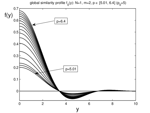
Figure 1. The first profile $f_{0}(y)$ of (3.2) for $N=1$, $m=2$ and $p\in[5.01,6.4]$.

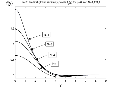
Figure 2. The first radially symmetric solution $f_{0}(y)$ of (2.2) for $m=2$, $p=6$, and dimensions $N=1$, 2, 3, 4.

3.3. $p$-branches and further even profiles

More delicate results are shown in Figure 3, where we present the global $p_{0}$-branch, initiated at $p=5^{+}$ and extended up to $p=200$. In particular, this shows that

(3.13) $$\|f_{0}\|_{\infty}\equiv f_{0}(0)\to 1^{+}\quad\mbox{as}\quad p\to+\infty,$$

an asymptotic phenomenon with a possible difficult logarithmically perturbed behaviour that was discovered and studied in [17, § 5] for another model (3.2) with the monotone nonlinearity $|f|^{p-1}f$. The deformation of the profile $f_{0}$ on the same interval $p\in[5.01,200]$ is shown in Figure 4, again confirming (3.13).

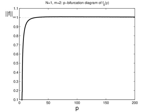
Figure 3. $p_{0}$-branch of $f_{0}$ for $N=1$, $m=2$, extended for $p\in[5.01,200]$.

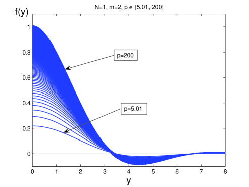
Figure 4. $p$-deformation of $f_{0}$ from Figure 3; $N=1$, $m=2$, $p\in[5.01,200]$.

We next study the extension of the $p_{0}$-branch for $p<p_{0}=5$. The transition through the first transcritical bifurcation at $p=p_{0}=5$ is explained in Figure 5, which shows a clear spatial similarity of $f_{0}(y)\sim\pm\psi_{0}(y)=\pm F(y)$ along both limits $p\to p_{0}^{\pm}=5^{\pm}$, according to (2.25) for $l=0$.

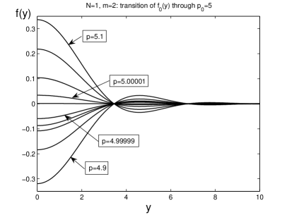
Figure 5. Transition of $f_{0}(y)$ to $f_{2}(y)$ of (3.2) for $N=1$, $m=2$ for $p\approx 5^{\pm}$.

The global $p_{2}$-branch, which is an extension of the positive $p_{0}$-one in Figure 4, is shown in Figure 6 while the corresponding deformation of $f$’s in Figure 7. It turns out that it ends up at the next (even) bifurcation point

(3.14) $$\textstyle{p=p_{2}=1+\frac{4}{1+2}=\frac{7}{3}=2.3333...\,,}$$

so that the branch is expected to be continued for $p<p_{2}=\frac{7}{3}$ in a “positive” way, etc.

To justify such transcritical bifurcations at $p=p_{l}$ for even $l\geq 2$, in Figure 8, we present a transition through $p=p_{2}=\frac{7}{3}\,.$ Similarly, in Figure 9, we show transition from $f_{4}(y)$ for $p=1.85>p_{4}=1+\frac{4}{5}=1.8$ to $f_{6}(y)$ for $p=1.75<p_{4}$.

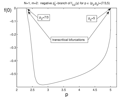
Figure 6. $p_{2}$-branch of $f_{2}$ for $N=1$, $m=2$, extended for $p\in(p_{2},p_{0})$.

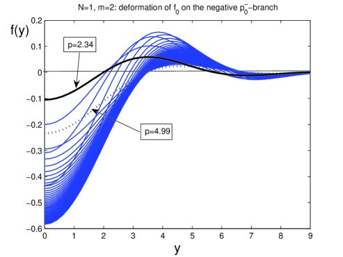
Figure 7. $p$-deformation of $f_{2}$ from Figure 6; $N=1$, $m=2$, $p\in(p_{2},p_{0})$.

Thus, according to the results given above, we expect that there is a continuous deformation along each connected branch of $f_{0}$ into $f_{2}$, $f_{2}$ into $f_{4}$, $f_{4}$ into $f_{6}$, etc., i.e., there exists a unique global $p$-branch of even similarity profiles. Hence, we observe that all connected branches have similar shapes with always two bifurcation points involved: the right-hand end point $p=p_{4k}$ and the left-hand end one $p_{4k+2}$.

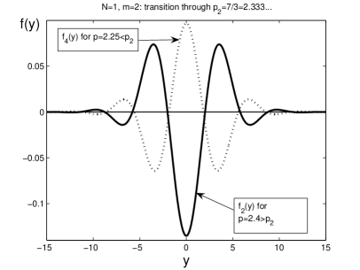
Figure 8. Transition of $f_{2}$ for $p=2.4>p_{2}$ into $f_{4}$ for $p=2.25<p_{2}$, where spatial shape of both mimics the eigenfunction $\psi_{2}(y)$ according to (2.25).

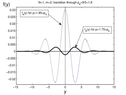
Figure 9. Transition of $f_{4}$ for $p=1.85>p_{4}$ into $f_{6}$ for $p=1.75<p_{4}$, where spatial shape of both mimics the eigenfunction $\psi_{4}(y)$ according to (2.25).

3.4. “Approximate” Sturmian zero property

Let us comment on the “Sturmian property” of similarity profiles $\{f_{l}(y)\}$. Figures 5 and 8 indicate that, regardless the oscillatory exponential tails, each profile $f_{l}(y)$ has a clear “approximate” (“nonlinear”) Sturmian structure and exhibits $l+1$ dominant extrema (meaning $l$ “transversal” zeros in between). In a rigorous mathematical sense, such properties are known to hold for the second-order problems. In [20], where (1.1) was studied, Sturmian properties were connected with the category of the functional subset for each $f_{l}$, being the corresponding min-max critical point of the functional, since the category assumes using the reflection of the functions $(\cdot)\mapsto-(\cdot)$ and hence the nodal sets of $f_{l}(y)$ gets more and more complicated as $l$ increases. However, in the present non-variational case, we cannot use even those rather obscure issues, though numerical evidence clearly suggests that the approximate Sturmian nodal properties persist in both variational and non-potential problems. Honestly, we do not know, which “mathematical/functional structures” can be responsible for such a hugely stable Sturmian-like phenomena, and this remains a challenging open problem of nonlinear operator theory.

For the higher-order equations, some extra mathematical reasons for Sturmian properties to persist in an approximate fashion are discussed in [17, § 4.4]. These can be attributed to the fact that the principal part of (3.2) contains the iteration of two positive operators

$$-D^{4}_{y}=-(-D^{2}_{y})(-D^{2}_{y}),$$

and for such pure higher-order operators Sturm’s zero property is true [11]. Then the linear perturbations affect non-essential zeros in the exponential tails only. No rigor justification of such a conclusion is available still.

4. Towards odd non-symmetric profiles and their $p$-branches

4.1. An auxiliary discussion

We begin with noting that, for such fourth-order nonlinear ODEs (3.2) with a clearly principal non-coercive operator, for any $p>1$, we expect to have, at least, a countable set of different solutions (as in [17, 18, 19]).

However, in all our previous studies of higher-order elliptic ODE problems, [17, 18, 19], exactly half of such solutions were odd functions of $y$ (in 1D; in the radial symmetry, obviously, odd profiles are not admitted). In the present case, the profiles $f_{1}(y)$, $f_{3}(y)$,… , are not odd (anti-symmetric), since the ODE (3.2), unlike that for (1.6), does not admit the corresponding symmetry

(4.1) $$f\mapsto-f,\quad y\mapsto-y.$$

Bearing in mind the multiplicity bifurcation results in Section 2.5, one concludes that other profiles must be non-symmetric in any odd sense. Notice that precisely that explains the bifurcation expansion (2.38), where the leading term is odd via $\psi_{1}(y)$, while there exists always an even correction via $\psi_{2}(y)$.

We first check some analytical issues concerning such unusual similarity profiles. Thus, we shoot from $y=+\infty$ using the same bundle as (3.9), with the coefficients $C^{+}_{1,2}$,

(4.2) $$\textstyle{f(y)\sim{\mathrm{e}}^{-\frac{a_{0}}{2}\,y^{4/3}}\big{[}C^{+}_{1}\cos\big{(}\frac{a_{0}\sqrt{3}}{2}\,y^{\frac{4}{3}}\big{)}+C^{+}_{2}\sin\big{(}\frac{a_{0}\sqrt{3}}{2}\,y^{\frac{4}{3}}\big{)}\big{]},\quad\mbox{where}\quad a_{0}=3\cdot 2^{-\frac{8}{3}}.}$$

Evidently, most of such solutions $f=f(y;C_{1}^{+},C_{2}^{+})$ will blow-up at some finite $y_{0}=y_{0}(C_{1}^{+},C_{2}^{+})$ according to the following asymptotics: as $y\to y_{0}^{+}$,

(4.3) $$\begin{matrix}f^{(4)}=|f|^{p}(1+o(1))\quad\Longrightarrow\quad f(y)=C_{0}(y-y_{0})^{-\frac{4}{p-1}}(1+o(1)),\vskip 3.0pt plus 1.0pt minus 1.0pt\\ \mbox{where}\quad C_{0}^{p-1}=\frac{4}{p-1}\big{(}\frac{4}{p-1}+1\big{)}\big{(}\frac{4}{p-1}+2\big{)}\big{(}\frac{4}{p-1}+3\big{)}.\end{matrix}$$

Therefore, in order to have a global profile, we have to require that

(4.4) $$y_{0}(C_{1}^{+},C_{2}^{+})=-\infty.$$

Once we have got such a global solution defined for all $y\in\mathbb{R}$, we then need to require that, at $y=-\infty$, the algebraic decay component (3.10) therein vanishes, i.e.,

(4.5) $$C_{0}^{-}(C_{1}^{+},C_{2}^{+})=0.$$

We, thus, again arrive at a system of two algebraic equation (4.4), (4.5), where the result of Proposition 3.2 applies directly to guarantee that the total number of possible solutions is not more than countable.

In Figure 10, as a first typical example, we show a non-symmetric “dipole-like” profile, denoted by $f_{3}(y)$ (see below why such a subscript) for $p=2.7$, which with a sufficient accuracy $\sim 10^{-5}$ satisfies the identity (3.4). It turned out that this identity can be used as a “blueprint” for checking the quality in some worse-converging cases.

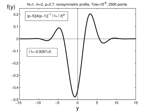
Figure 10. A non-symmetric profile $f_{3}(y)$ for $p=2.7$, well satisfying the identity (3.4).

4.2. $p$-branch of $f_{3}$: from $p_{1}=3$ to a saddle-node bifurcation

Starting from the profile $f_{3}$ for $p=2.7$ in Figure 10, we perform a continuation in the parameter $p$ to get to the bifurcation origin of this $p$-branch. Not that surprisingly (cf. Section 2.5), we observe in Figure 11(a) that the corresponding bifurcation branch, with certain accuracy, goes to the odd bifurcation point (1.5), with $l=1$:

(4.6) $$\textstyle{p_{1}=1+\frac{4}{2}=3.}$$

In this calculation, we take the continuation step $\Delta p=10^{-2}$ (then the calculation takes a couple of hours), so, as seen, we cannot approach closely to this bifurcation point. To see approaching $p=p_{1}$ more clearly, we, in addition, took the continuation step $\Delta p=10^{-4}$ (the calculation of the full branch then took about 16 hours) and observe approaching $p_{1}=3$ up to $p=2.9991$, so that existence of such a “forbidden” earlier bifurcation is without any doubt. Figure 11(b) clearly shows that, as $p\to p_{1}^{-}=3$, the profile $f_{3}(y)$ (the bold dashed line at $p=2.998$)) takes a typical “dipole” behaviour governed by the second eigenfunction from (2.10):

(4.7) $$\textstyle{\psi_{1}(y)=-F^{\prime}(y),}$$

where $F(|y|)$ is the even “bi-harmonic Gaussian” satisfying (2.5) for $m=2$. Therefore, this $f_{3}(y)\sim C(p)\psi_{1}(y)$, with some (unknown still) constant $C(p)$, looks like a standard dipole for the Gaussian for $m=1$

(4.8) $$\textstyle{\psi_{1}(y)=\frac{1}{2\sqrt{4\pi}}\,y\,{\mathrm{e}}^{-y^{2}/4},}$$

but it has oscillatory tails and further dominant positive and negative humps.

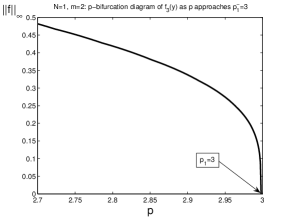
(a) $p$-bifurcation branch of $f_{3}$

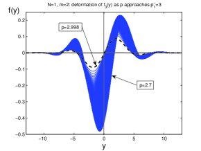
(b) deformation of $f_{3}$

Figure 11. $p$-bifurcation branch of $f_{3}$ (a), and its deformation (b) for $p\in[2.7,2.924]$.

Extending this $p$-branch of $f_{3}$ for $p<2.7$, we observe existence of a saddle-node bifurcation at some $p=p_{s-n}$, where we obtain the estimate

(4.9) $$\framebox{$2.6148<p_{s-n}\leq 2.6149,$}$$

by using again the step $\Delta p=10^{-4}$. The profiles $f_{3}$ close to $p_{s-n}$ are shown in Figure 12.

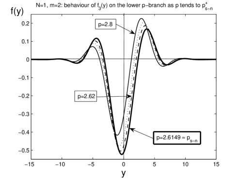
Figure 12. Non-symmetric profiles $f_{3}(y)$ close to the saddle-node bifurcation (4.9).

The lower bifurcation branch of $f_{3}$ is shown in Figure 13. The corresponding upper bifurcation branch is shown in Figure 14, while the corresponding deformation of $f_{3}$ is presented in Figure 15.

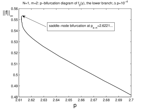
Figure 13. The lower bifurcation branch of the non-symmetric profile $f_{3}(y)$ for $p\in[2.6149,2.7]$.

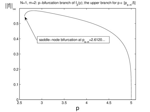
Figure 14. The upper bifurcation branch of the non-symmetric profile $f_{3}(y)$ for $p\in[2.6149,5]$.

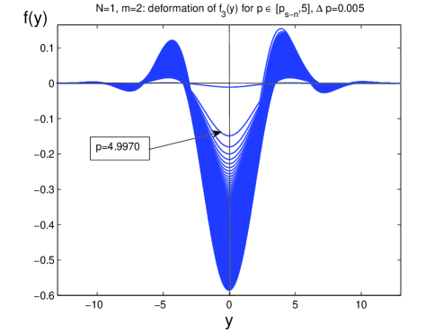
Figure 15. Deformation of the non-symmetric profile $f_{3}(y)$ for $p\in[2.6149,5]$.

Quite surprisingly, the upper bifurcation branch in Figure 14 ends up at the previous bifurcation point $p_{0}=5$! Comparing with Figure 6 for symmetric even profiles, we thus obtain two different bifurcation branches (of symmetric and non-symmetric) solutions originated at $p=5^{-}$. It is worth mentioning that the kernel of the linearized operator at $p=5$ is one-dimensional. We still do not have a proper explanation of such a hard and unusual bifurcation phenomenon. However, the case $l=0$ is not degenerate by (2.22), so it seems one cannot create a bifurcation approach similar to that in Section 2.5. This remains an open problems

5. Second countable family: global linearized patterns

5.1. Stable manifold patterns

This construction is similar to that for $m=1$ and again relies on stable manifold [28] and Hermitian spectral theory for the operator pair $\{{\bf B},{\bf B}^{*}\}$ in Section 2.2. We perform the same scaling of a global solution $u(x,t)$ of (1.2) for $t\gg 1$,

(5.1) $$\textstyle{u(x,t)=t^{-\frac{1}{p-1}}\,v(y,\tau),\quad y=x/{t^{\frac{1}{2m}}},\quad\tau=\ln t,\quad\mbox{where}\quad}$$

(5.2) $$\textstyle{v_{\tau}={\bf A}(v)\equiv-(-\Delta)^{m}v+\frac{1}{2m}\,y\cdot\nabla v+\frac{1}{p-1}\,v+|v|^{p},\quad\mbox{so}}$$

(5.3) $$\textstyle{{\bf A}^{\prime}(0)={\bf B}+c_{1}I,\quad c_{1}=\frac{1}{p-1}-\frac{N}{2m}=\frac{N(p_{0}-p)}{2(p-1)}>0\,\,\,\mbox{for}\,\,\,p<p_{0}.}$$

Thus, ${\bf A}^{\prime}(0)$ has the infinite-dimensional stable subspace:

(5.4) $$E^{s}={\rm Span}\{\psi_{\beta}:\,\,\,\lambda_{\beta}+c_{1}<0,\,\,\mbox{i.e.,}\,\,|\beta|>2c_{1}\}.$$

Using the above spectral properties of ${\bf B}$ [9], similar to [20, § 5], by invariant manifold theory for parabolic equations [28, Ch. 9], we arrive at the following (see also [15, 17]):

Proposition 5.1.

For any multiindex $\beta$ satisfying $|\beta|=l>2c_{1}$, equation $(\ref{L2m})$ admits global solutions with the behaviour, as $\tau\to+\infty$,

(5.5) $$v_{\beta}(y,\tau)={\mathrm{e}}^{(\lambda_{\beta}+c_{1})\tau}\varphi_{\beta}(y)(1+o(1)),\quad\mbox{where}\quad\varphi_{\beta}\in{\rm Span}\{\psi_{\beta}:\,\,\,|\beta|=l\},\,\,\,\varphi_{\beta}\not=0.$$

In the original variables (5.1), the global patterns (5.5) take the form:

(5.6) $$\textstyle{u_{\beta}(x,t)=t^{-\frac{N+|\beta|}{2m}}\,\varphi_{\beta}\big{(}\frac{x}{t^{1/2m}}\big{)}(1+o(1))\quad\mbox{as}\quad t\to+\infty.}$$

5.2. Centre manifold patterns

Unlike the simpler case $m=1$ in [20, § 5.2], for the present $m\geq 2$, such patterns do exist. Performing a model 1D analysis of the equation (5.2), as in [20, § 5], we conclude that such patterns may occur if

(5.7) $$\lambda_{\beta}+c_{1}=0\quad\Longrightarrow\quad l=|\beta|=2mc_{1}>0,\quad\mbox{or}\quad p=p_{l}.$$

Studying the centre manifold behaviour of the simplest 1D type

(5.8) $$v(\tau)=a_{l}(\tau)\psi_{l}+w^{\bot}\quad\mbox{as}\quad\tau\to+\infty,$$

we obtain from (5.2) the following equation for the expansion coefficient:

(5.9) $$\dot{a}_{l}=\kappa_{l}\,|a_{l}|^{p}(1+o(1)),\quad\mbox{where}\quad\kappa_{l}=\langle|\psi_{l}|^{p},\psi_{l}^{*}\rangle\,\,(\neq 0),$$

which admits global bounded orbits. For instance, noting that $\kappa_{0}>0$, one obtains the behaviour

(5.10) $$a_{0}(\tau)=-[\kappa_{0}(p-1)]^{-\frac{1}{p-1}}\,\tau^{-\frac{1}{p-1}}(1+o(1))\quad\mbox{as}\quad\tau\to+\infty\quad(p=p_{0}).$$

Similarly, the same estimate is derived for any $l\geq 0$ provided that $\kappa_{l}\not=0$. Finally, this means that, at such critical values $p=p_{l}$, we expect the following logarithmically perturbed patterns:

(5.11) $$\textstyle{u_{l}(x,t)\sim-{\rm sign}\,\kappa_{l}\,\big{[}\frac{2m|\kappa_{l}|}{N+l}\big{]}^{-\frac{N+l}{2m}}\,\big{(}t\ln t\big{)}^{-\frac{N+l}{2m}}\psi_{l}\big{(}\frac{x}{t^{1/2m}}\big{)}\quad\mbox{as}\quad t\to+\infty.}$$

For the $M$-dimensional eigenspace for $l\geq 1$, we obtain the decomposition

(5.12) $$\textstyle{v(y,\tau)=\sum\limits_{|\beta|=l}a_{\beta}(\tau)\psi_{\beta}(y)+w^{\bot}(y,\tau),}$$

that leads to a system of ODEs for the expansion coefficients $\{a_{\beta}(\tau)\}_{|\beta|=l}$:

(5.13) $$\textstyle{\dot{a}_{\gamma}=\big{\langle}\big{|}\sum_{|\beta|=l}a_{\beta}(\tau)\psi_{\beta}\big{|}^{p},\psi_{\gamma}^{*}\big{\rangle}+...\,,\quad|\gamma|=l.}$$

Assuming the natural “homogenuity” of this centre subspace behaviour:

(5.14) $$\textstyle{a_{\beta}(\tau)=\hat{a}_{\beta}\,\tau^{-\frac{N+l}{2m}}(1+o(1))\quad\mbox{as}\quad\tau\to+\infty,\quad|\beta|=l,}$$

where $\{\hat{a}_{\beta}\}$ are constants, (5.13) reduces to an algebraic system (cf. the bifurcation one (2.29)) of the usual form:

(5.15) $$\textstyle{\hat{a}_{\gamma}=-\frac{2m}{N+l}\big{\langle}\big{|}\sum_{|\beta|=l}\hat{a}_{\beta}\psi_{\beta}\big{|}^{p},\psi_{\gamma}^{*}\big{\rangle},\quad|\gamma|=l.}$$

General solvability properties of (5.15), except some obvious elementary solutions, and sharp multiplicity results are unknown. Of course, as above, (5.15) is not variational.

Again, as for $m=1$, we arrive at two countable families of global patterns: the nonlinear (2.1) and the linearized (5.6) ones. Since the rescaled equation (5.2) is not a gradient system in any weighted space, their evolution completeness remains entirely open, though may be expected.

References

- [1] R. Bari and B. Rynne, Solution curves and exact multiplicity results for th order boundary value problems, J. Math. Anal. Appl., 292 (2004), 17–22.
- [2] M. Berger, Nonlinearity and Functional Analysis, Acad. Press, New York, 1977.
- [3] C.J. Budd, V.A. Galaktionov, and J.F. Williams, Self-similar blow-up in higher-order semilinear parabolic equations, SIAM J. Appl. Math., 64 (2004), 1775–1809.
- [4] M.S. Birman and M.Z. Solomjak, Spectral Theory of Self-Adjoint Operators in Hilbert Space, D. Reidel, Dordrecht/Tokyo, 1987.
- [5] R. Czaja and C. Rocha, Transversality in scalar reaction-diffusion equations on a circle, J. Differ. Equat., 245 (2008), 692–721.
- [6] E.A. Coddington and N. Levinson, Theory of Ordinary Differential Equations, McGraw-Hill Book Company, Inc., New York/London, 1955.
- [7] K. Deimling, Nonlinear Functional Analysis, Springer-Verlag, Berlin/Tokyo, 1985.
- [8] Yu.V. Egorov, V.A. Galaktionov, V.A. Kondratiev, and S.I. Pohozaev, On the necessary conditions of existence to a quasilinear inequality in the half-space, Comptes Rendus Acad. Sci. Paris, Série I, 330 (2000), 93-98.
- [9] Yu.V. Egorov, V.A. Galaktionov, V.A. Kondratiev, and S.I. Pohozaev, Global solutions of higher-order semilinear parabolic equations in the supercritical range, Adv. Differ. Equat., 9 (2004), 1009–1038.
- [10] S.D. Eidelman, Parabolic Systems, North-Holland Publ. Comp., Amsterdam/London, 1969.
- [11] U. Ellias, Eigenvalue problems for the equation , J. Differ. Equat., 29 (1978), 28–57.
- [12] M. Escobedo and O. Kavian, Variational problems related to self-similar solutions of the heat equation, Nonl. Anal., TMA, 11 (1987), 1103–1133.
- [13] B. Fiedler and C. Rocha, Connectivity and design of planar global attractors of Sturm type. II: Connection graphs, J. Differ. Equat., 244 (2008), 1255–1286.
- [14] M.V. Fedoryuk, Singularities of the kernels of Fourier integral operators and the asymptotic behaviour of the solution of the mixed problem, Russian Math. Surveys, 32 (1977), 67–120.
- [15] V.A. Galaktionov, Critical global asymptotics in higher-order semilinear parabolic equations, Int. J. Math. Math. Sci., 60 (2003), 3809–3825.
- [16] V.A. Galaktionov, Geometric Sturmian Theory of Nonlinear Parabolic Equations and Applications, ChapmanHall/CRC, Boca Raton, Florida, 2004.
- [17] V.A. Galaktionov and P.J. Harwin, Non-uniqueness and global similarity solutions for a higher-order semilinear parabolic equation, Nonlinearity, 18 (2005), 717–746.
- [18] V.A. Galaktionov, E. Mitidieri, and S.I. Pohozaev, Variational approach to complicated similarity solutions of higher-order nonlinear evolution equations of parabolic, hyperbolic, and nonlinear dispersion types, In: Sobolev Spaces in Mathematics. II, Appl. Anal. and Part. Differ. Equat., Series: Int. Math. Ser., Vol. 9, V. Maz’ya Ed., Springer, New York, 2009 (an extended version in arXiv:0902.1425).
- [19] V.A. Galaktionov, E. Mitidieri, and S.I. Pohozaev, Variational approach to complicated similarity solutions of higher-order nonlinear PDEs. II, Nonl. Anal.: RWA, 12 (2011), 2435–2466 (arXiv:1103.2643).
- [20] V.A. Galaktionov, E. Mitidieri, and S.I. Pohozaev, Classification of global and blow-up sign-changing solutions of a semilinear heat equation in the subcritical Fujita range I. Second-order diffusion, submitted.
- [21] V.A. Galaktionov and S.I. Pohozaev, Existence and blow-up for higher-order semilinear parabolic equations: majorizing order-preserving operators, Indiana Univ. Math. J., 51 (2002), 1321–1338.
- [22] V.A. Galaktionov and J.L. Vazquez, A Stability Technique for Evolution Partial Differential Equations. A Dynamical Systems Approach, Birkhäuser, Boston/Berlin, 2004.
- [23] V.A. Galaktionov and J.F. Williams, On very singular similarity solutions of a higher-order semilinear parabolic equation, Nonlinearity, 17 (2004), 1075–1099.
- [24] R. Joly and G. Raugel, Generic hyperbolicity of equilibria and periodic orbits of the parabolic equation on a circle, Trans. Amer. Math. Soc., 362 (2010), 5189–5211.
- [25] T. Kato, Perturbation Theory for Linear Operators, Springer-Verlag, Berlin/ New York, 1976.
- [26] M.A. Krasnosel’skii, Topological Methods in the Theory of Nonlinear Integral Equations, Pergamon Press, Oxford/Paris, 1964.
- [27] M.A. Krasnosel’skii and P.P. Zabreiko, Geometrical Methods of Nonlinear Analysis, Springer-Verlag, Berlin/Tokyo, 1984.
- [28] A. Lunardi, Analytic Semigroups and Optimal Regularity in Parabolic Problems, Birkhäuser, Basel/Berlin, 1995.
- [29] B. Rynn, Global bifurcation for th-order boundary value problems and infinitely many solutions of superlinear problems, J. Differ. Equat., 188 (2003), 461–472.