Contact intensity and extended hydrodynamics in the BCS-BEC crossover

Abstract

In the first part of this chapter we analyze the contact intensity $C$, which has been introduced by Tan [Ann. Phys. 323, 2952 (2008)] and appears in several physical observables of the strongly correlated two-component Fermi gas. We calculate the contact $C$ in the full BCS-BEC crossover for a uniform superfluid Fermi gas by using an efficient parametetrization of the ground-state energy. In the case of harmonic confinement, within the Thomas-Fermi approximation, we derive analytical formulas of $C$ in the three relevant limits of the crossover. In the second part of this chapter we discuss the extended superfluid hydrodynamics we have recently proposed to describe static and dynamical collective properties of the Fermi gas in the BCS-BEC crossover. In particular we show the relation with the effective theory for the Goldstone field derived by Son and Wingate [Ann. Phys. 321, 197 (2006)] on the basis of conformal invariance. By using our equations of extended hydrodynamics we determine nonlinear sound waves, static response function and structure factor of a generic superfluid at zero temperature.

1 Contact intensity

It has been proved by Tan tan1 that the momentum distribution $\rho_{\sigma}(k)$ in an arbitrary system consisting of fermions in two spin states ($\sigma=\uparrow,\downarrow$) with a large scattering length has a tail that falls off as

$$\rho_{\sigma}(k)\sim{C\over k^{4}}$$ (1)

for $k\to\infty$, where $C$ is the so-called contact intensity tan1 . Here large s-wave scattering length $a$ means that $|a|\gg r_{0}$, where $r_{0}$ is the effective interaction radius. Under this condition Tan tan1 has shown that $C$ is related to the total energy $E$ of the Fermi system by the rigorous expression

$$C={4\pi ma^{2}\over\hbar^{2}}{dE\over da}\;,$$ (2)

where the derivative is taken under constant entropy and, in general, $C$ depends on the number $N$ of fermions, the scattering length $a$ and the parameters of the trapping potential tan2 ; tan3 . Remarkably, Eqs. (1) and (2) work also at finite temperature and in this case $C$ will be a function of $T$ tan2 ; leggett . Tan has also derived, for finite scattering lengths, a generalized virial theorem and a generalized pressure relation where the contact $C$ appears tan3 . The contact intensity $C$ appears also in other physical observables of the strongly correlated Fermi system. For instance, the radio-frequency spectroscopy shift is proportional to $C$ zwerger ; zwierlein ; pieri ; pieri2 , and the same happens to the photoassociation rate castin . Very recently, it has been shown that the contact $C$ gives the asymptotic tail behavior of the shear viscosity as a function of the frequency braaten3 .

Using the methods of quantum field theory, Braaten and Platter have rederived braaten1 ; braaten11 the Tan’s universal relations tan1 ; tan2 ; tan3 . In addition, they have shown that the contact intensity can be written as

$$C=\int g^{2}\langle{\hat{\psi}}_{\uparrow}^{+}({\bf r}){\hat{\psi}}_{\downarrow}^{+}({\bf r}){\hat{\psi}}_{\downarrow}({\bf r}){\hat{\psi}}_{\uparrow}({\bf r})\rangle\ d^{3}{\bf r}\;,$$ (3)

where ${\hat{\psi}}_{\sigma}({\bf r})$ is the fermionic field operator of spin $\sigma$ and $g=4\pi a/(1-(2ak_{cut}/\pi))$ is the bare coupling constant of the Fermi pseudo-potential interaction, with $k_{cut}$ the ultraviolet wavenumber cutoff braaten1 ; braaten2 . Braaten and Platter have also shown that the number ${\cal N}_{pair}({\bf r})$ of pairs of fermions with opposite spins in a small ball of volume $4\pi s^{3}/3$ centered at the point ${\bf r}$ scales as $s^{4}{\cal C}({\bf r})/2$ for $s\to 0$, where ${\cal C}({\bf r})=g^{2}\langle{\hat{\psi}}_{\uparrow}^{+}({\bf r}){\hat{\psi}}_{\downarrow}^{+}({\bf r}){\hat{\psi}}_{\downarrow}({\bf r}){\hat{\psi}}_{\uparrow}({\bf r})\rangle$ is the contact density braaten1 ; braaten2 .

Explicit expressions of the universal quantity $C$ have been derived by Tan tan1 for a uniform superfluid Fermi gas at zero temperature only in three limits: the Bardeen-Cooper-Schrieffer (BCS) limit of weakly bound Cooper pairs, the unitarity limit of infinite scattering length, and the Bose-Einstein condensate (BEC) limit of weakly-interacting bosonic molecular pairs.

In this section we calculate the contact $C$ as a function of the inverse scattering parameter $1/(k_{F}a)$ for a uniform superfluid Fermi gas in the full BCS-BEC crossover. To perform this calculation we use an efficient fitting formula of the ground-state energy nick ; nick2 and the Tan’s equation (2). We find that the contact $C$ has a maximum close to the unitarity limit of infinite scattering length. We also consider the interacting Fermi system under harmonic confinement. For this superfluid Fermi cloud we derive analytical formulas of the contact $C$ in the three relevant limits of the crossover.

1.1 Uniform superfluid Fermi gas at zero temperature

In the case of a zero-temperature uniform two-component superfluid Fermi gas of total density $n=n_{\uparrow}+n_{\downarrow}$ ($n_{\uparrow}=n_{\downarrow}$), large scattering length $a$ ($a\gg r_{0}$) in a volume $V$, the energy density can be written as

$${E\over V}={3\over 5}n\epsilon_{F}f({1\over k_{F}a})\;,$$ (4)

where $f(y)$ is a universal function of inverse interaction parameter $y=1/(k_{F}a)$, with $\epsilon_{F}=\hbar^{2}k_{F}^{2}/(2m)$ the Fermi energy and $k_{F}=(3\pi^{2}n)^{1/3}$ the Fermi wave numberleggett . We observe that at finite finite temperature $T$ the function $f(y)$ is substituted by a more general universal function $\Phi(y,t)$, where $t=T/\epsilon_{F}$ is the scaled temperature. $\Phi(y,t)$ has been studied with Monte Carlo methods by Bulgac, Drut, and Migierski bulgac ; bulgac01 , but only in the unitarity limit ($y=0$).

It is straightforward to derive from Eq. (2) the expression of the contact density

$${C\over V}=-{6\pi\over 5}k_{F}n{df\over dy}\;.$$ (5)

The behavior of $f(y)$ is well known in three relevant limits:

$$f(y)=\left\{\begin{array}[]{cc}1+{10\over 9\pi}{1\over y}+O(1/y^{2})\;,&y\ll-1\\ \xi-\zeta y+O(y^{2})\;,&-1\ll y\ll 1\\ {5{\cal P}\over 18\pi}{1\over y}+O(1/y^{5/2})\;,&y\gg 1\end{array}\right.$$ (6)

In fact, in the weakly attractive limit ($y\ll-1$) one expects a BCS Fermi gas of weakly bound Cooper pairs. As the superfluid gap correction is exponentially small, the function $f(y)$ follows the Fermi-gas expansion p15 ; p151 . In the so-called unitarity limit ($y=0$) one expects that the energy per particle is proportional to that of a non-interacting Fermi gas with the universal constant $\xi$ given by $\xi\simeq 0.42$ giorgini . Note that more recent auxiliary-field Monte Carlo results gandolfi predict a smaller value for $\xi$, namely $\xi\simeq 0.38$, while the experiment performed at Ecole Normale Superieure salomon suggests $\xi\simeq 0.40$. The first correction to this behavior, shown in Eq. (6), has been estimated from Monte Carlo data with $\zeta\simeq 1$ bertsch . In the weak BEC limit ($y\gg 1$) one expects a weakly repulsive Bose gas of dimers. Such Bose-condensed molecules of mass $m_{M}=2m$ and density $n_{M}=n/2$ interact with a positive scattering length $a_{M}={\cal P}a$ with ${\cal P}\simeq 0.6$, as predicted by Petrov et al. p16 . In this regime, after subtraction of the molecular binding energy, the function $f(y)$ follows the Bose-gas expansion p17 . It is easy to obtain the contact intensity $C$ by using Eqs. (2) and (6) in the relevant limits of the crossover. One finds

$${C\over V}=\left\{\begin{array}[]{cc}{4\over 3}k_{F}^{3}na^{2}+O(a^{3})\;,&y\ll-1\\ {6\pi\over 5}k_{F}n\zeta+O(1/a)\;,&-1\ll y\ll 1\\ {{\cal P}\over 3}k_{F}^{3}na^{2}+O(a^{7/2})\;,&y\gg 1\end{array}\right.$$ (7)

in agreement with the previous determinations of Tan tan1 and Werner, Tarruell and Castin castin . Notice that in the BEC limit we have removed the binding energy of molecules. Moreover, very recently finite temperature corrections to Eq. (7) were given in Ref. finite-t .

1.2 Contact intensity in the BCS-BEC crossover

Now we want to calculate the behavior of $C$ in the full BCS-BEC crossover. In 2005 we have proposed nick the following analytical fitting formula

$$f(y)=\alpha_{1}-\alpha_{2}\arctan{\left(\alpha_{3}\;y\;{\beta_{1}+|y|\over\beta_{2}+|y|}\right)}\;,$$ (8)

interpolating the Monte Carlo energy per particle giorgini and the limiting behaviors for large and small $|y|$. Eq. (8) is very reliable nick ; nick2 and it has been successfully used by various authors for studying grund-state and collective properties of this superfluid Fermi system vari ; vari2 ; vari3 ; vari4 ; vari5 . The parameter $\alpha_{1}$ is fixed by the value $\xi$ of $f(y)$ at $y=0$, the parameter $\alpha_{2}$ is fixed by the value of $f(y)$ at $y=\infty$, and $\alpha_{3}$ is fixed by the asymptotic $1/y$ coefficient of $\epsilon(y)$ at large $|y|$. The ratio $\beta_{1}/\beta_{2}$ is determined by the linear behavior $\zeta$ of $\epsilon(y)$ near $y=0$. The value of $\beta_{1}$ is then determined by minimizing the mean square deviation from the Monte-Carlo data. Of course, we have considered two different set of parameters: one set in the BCS region ($y<0$) and a separate set in the BEC region ($y>0$) nick . Table 1 of nick reports the values of these parameters, with $\zeta=\zeta_{-}=1$ in the BCS region but $\zeta=\zeta_{+}=1/3$ in the BEC region.

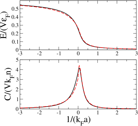
Figure 1: Upper panel: Scaled ground-state energy $E/(V\epsilon_{F})$ of the uniform Fermi gas as a function of the inverse interaction parameter $1/(k_{F}a)$ in the BCS-BEC crossover. Lower panel: Scaled contact intensity $C/(Vk_{F}n)$ of the Fermi system as a function of the inverse interaction parameter $1/(k_{F}a)$. Here $V$ and $n=N/V$ are the volume and the density of the Fermi gas, $k_{F}=(3\pi^{2}n)^{1/3}$ is the Fermi wave number and $\epsilon_{F}=\hbar^{2}k_{F}^{2}/(2m)$ is the Fermi energy. Two different parametrization of the universal function $f(y)$: solid lines are obtained with Eq. (8), while dashed lines are calculated using the Pade approximant of kim .

Here we use Eq. (8) to calculate the contact density given by Eq. (5), but contrary to nick , we choose $\zeta_{+}=\zeta_{-}=\zeta=1$ to ensure the continuity of $f^{\prime}(y)$ at $y=0$. Notice that the recent experimental results obtained at Ecole Normale Superieure salomon indeed suggest the continuity of $f^{\prime}(y)$ at $y=0$. In this way, in the BEC region $\beta_{2}=0.1517$ while $\beta_{1}$ is unchanged (see Table. 1 of nick ). In the upper panel of Fig. 1 we plot the ground-state energy $E$ while in the lower panel we plot the contact $C$, both as a function of the inverse interaction parameter $y=1/(k_{F}a)$. For comparison, in addition to the data obtained with our method (solid lines), we insert also the results (dashed lines) one obtains using the Pade parametrization of $f(y)$ proposed by Kim and Zubarev kim . The figure shows that solid and dashed lines are always close each other, apart for $-1\ll y\leq 0$ where our fitting formula is smoother (and closer to the Monte Carlo data giorgini ). Moreover, the scaled contact $C/(Vk_{F}n)$ as a function of $1/(k_{F}a)$ has its maximum near to the unitarity limit $1/(k_{F}a)=0$: the position of the maximum is located at $1/(k_{F}a)\simeq 0.05$. Remarkably, the scaled contact has a behavior quite similar to the Landau’s critical velocity $v_{c}$ (at which there is the breaking of superfluid motion), calculated along the BCS-BEC crossover. In fact, also $v_{c}$ goes to zero for $y\to\pm\infty$ and it has a peak at $y\simeq 0.08$ comb . Clearly, the contact $C$ exhibits a maximum close to unitarity because we have subtracted the molecular binding energy contribution, given by $y^{2}$ in the BEC side ($y>0$). Including this energy term it is easy to show that $C$ increases monotonically from the BCS side to the BEC side, according the definition in Eq. (2). Nevertheless, as prevously stated, the radio-frequency spectroscopy shift is proportional to $C$, and its maximum around unitarity has been shown in Ref. zwierlein , where the same artificial subtraction has been adopted.

1.3 Trapped superfluid Fermi gas

Let us now consider the superfluid Fermi gas under an external harmonic confinement

$$U({\bf r})={1\over 2}m\omega^{2}(x^{2}+y^{2}+z^{2})\;.$$ (9)

In the limit of a large number $N$ of fermions we can use the local density (Thomas-Fermi) approximation flavio ; flavio2 ; flavio3 ; flavio4 ; flavio5 ; flavio6 ; flavio7 ; flavio8 and the energy of the system can be written as

$$E=\int\left\{{3\over 5}n({\bf r})\epsilon_{F}({\bf r})f({1\over k_{F}({\bf r})a})+n({\bf r})U({\bf r})\right\}\ d^{3}{\bf r}\ ,$$ (10)

where $\epsilon_{F}({\bf r})=\hbar^{2}k_{F}({\bf r})^{2}/(2m)$ is the local Fermi energy and $k_{F}=(3\pi^{2}n({\bf r}))^{1/3}$ is the local Fermi wave number. As in the uniform case, this expression is not very useful without the knowledge of the universal function $f(y)$.

The numerical calculation of the contact indensity $C$ for a harmonically trapped Fermi superfluid in the full BCS-BEC crossover by using Eqs. (2) and (8) is very demanding. Consequently, we calculate $C$ only in the three relevant limits of the BEC-BEC crossover. In these limits we obtain useful analytical expressions for the contact $C$.

BCS limit. In the BCS limit ($a\to 0^{-}$) from Eqs. (6) and (10) we find

$${dE\over da}={3\over 5}{10\over 9\pi}\int\left\{\epsilon_{F}({\bf r})n({\bf r})k_{F}({\bf r})\right\}\ d^{3}{\bf r}\;,$$ (11)

where $n({\bf r})$ is the density profile of the ideal Fermi gas in the harmonic potential (9), given by ideal

$$n({\bf r})={2\sqrt{2}\over 3\pi^{2}a_{H}^{3}}(3N)^{1/2}(1-{r^{2}\over r_{F}^{2}})^{3/2}\;,$$ (12)

where $r_{F}=\sqrt{2}(3N)^{1/6}a_{H}$ is the Fermi radius of the cloud, with $a_{H}=\sqrt{\hbar/(m\omega)}$ the characteristic harmonic length. Inserting this density profile into Eq. (11) and using Eq. (8) we get the contact intensity in the BCS limit:

$$C={4096\sqrt{2}\over 2835\pi}{1\over a_{H}}\left({a\over a_{H}}\right)^{2}(3N)^{3/2}\;.$$ (13)

Unitarity limit. In the unitarity limit ($a\to\pm\infty$) from Eqs. (6) and (10) we have

$${dE\over da}={3\over 5}{\zeta\over a^{2}}\int\left\{\epsilon_{F}({\bf r})n({\bf r}){1\over k_{F}({\bf r})}\right\}\ d^{3}{\bf r}\;,$$ (14)

where $n({\bf r})$ is the density profile of the unitary Fermi gas in the potential (9), namely flavio

$$n({\bf r})={2\sqrt{2}\over 3\pi^{2}a_{H}^{3}\xi^{3/4}}(3N)^{1/2}(1-{r^{2}\over r_{F}^{2}})^{3/2}\;,$$ (15)

where $r_{F}=\sqrt{2}\xi^{1/4}(3N)^{1/6}a_{H}$ is the Fermi radius of the unitary cloud. Inserting this density profile into Eq. (14) and using Eq. (8) we obtain the contact in the unitarity limit:

$$C={512\sqrt{2}\over 525}{\zeta\over\xi^{1/4}}{1\over a_{H}}(3N)^{7/6}\;.$$ (16)

BEC limit. In the BEC limit ($a\to 0^{+}$) it is straightforward to calculate the contact $C$. In fact, the explicit formula of the ground-state energy of the dilute BEC is well known review-bose and for a BEC of molecules it is given by

$$E={5\over 7}{\hbar\omega\over 2}\left({15{\cal P}a\over a_{H}}\right)^{2/5}\left({N\over 2}\right)^{7/5}\;,$$ (17)

where ${\cal P}\simeq 0.6$ and $N/2$ is the number of molecules. Then from Eq. (2) the contact intensity reads

$$C={2\pi\over 7}{1\over a_{H}}\left({15{\cal P}\over 2}\right)^{2/5}\left({aN\over a_{H}}\right)^{7/5}\;.$$ (18)

2 Extended superfluid hydrodynamics

In this section we discuss the extended Lagrangian density of superfluids we have proposed few years ago flavio and applied to study mainly the unitary Fermi gas flavio ; flavio2 ; flavio3 ; flavio4 ; flavio5 ; flavio6 ; flavio7 ; flavio8 . The internal energy density of this Lagrangian contains a term proportional to the kinetic energy of a uniform non interacting gas of fermions, plus a gradient correction of the von-Weizsacker form $\lambda\hbar^{2}/(8m)(\nabla n/n)^{2}$ von . This approach has been adopted for studying the quantum hydrodynamics of electrons by March and Tosi tosi , and by Zaremba and Tso tso . In the context of the BCS-BEC crossover, the gradient term is quite standard nick ; kim ; v2 ; v3 ; v4 ; v5 ; v6 ; v7 ; v8 . In particular we show the relation between our approach and the effective theory for the Goldstone field derived by Son and Wingate son , and improved by Manes and Valle valle , on the basis of conformal invariance. Finally, by using our equations of extended superfluid hydrodymics at zero temperature we calculate sound waves, static response function and structure factor of a generic superfluid.

The extended Lagrangian density of superfluids is given by

$${\cal L}=-\hbar\,{\dot{\theta}}\,n-{\hbar^{2}\over 2m}({\boldsymbol{\nabla}}\theta)^{2}\,n-{\cal E}(n,{\boldsymbol{\nabla}}n)-U({\bf r})\,n\;,$$ (19)

where $n({\bf r},t)$ is the local density, $U({\bf r})$ is the external potential acting on particles, and $m$ the mass of superfluid particles. In the case of superfluid bosons $\theta({\bf r},t)$ is the phase of the condensate order parameter, while in the case of superfluid fermions $\theta({\bf r},t)$ is half of the phase of the condensate order parameter (of Cooper pairs). ${\cal E}(n,{\boldsymbol{\nabla}}n)$ is the internal energy density of the system. Note that we are supposing that this equation of state ${\cal E}(n,{\boldsymbol{\nabla}}n)$ can depend not only on the local density $n({\bf r},t)$ but also on its space derivatives. For this reason we call (19) the extended superfluid Lagrangian. We stress that in the context of the BCS-BEC crossover the extended internal energy density could be written as

$${\cal E}(n,{\boldsymbol{\nabla}}n)={\cal E}_{0}(n)+\lambda{\hbar^{2}\over 8m}{({\boldsymbol{\nabla}}n)^{2}\over n}\;,$$ (20)

where

$${\cal E}_{0}(n)={3\over 5}n\epsilon_{F}f({1\over k_{F}a})$$ (21)

is the energy density discussed in the previous section (see Eq. (4)) which depends on the universal function $f(y)$ of the BCS-BEC crossover, while the second term is the gradient correction of the von-Weizsacker form flavio2 . In the BCS-BEC crossover we expect that $1/6\leq\lambda\leq 1/4$, where $\lambda=1/6$ is the appropriate value in BCS regime of weakly-interacting superfluid fermions of mass $m$ tosi ; tso , while $\lambda=1/4$ is the appropriate value in the deep BEC regime of weakly-interacting superfluid bosonic dimers of mass $2m$ flavio2 .

By using the Lagrangian density (19) the Euler-Lagrange equation

$${\partial{\cal L}\over\partial\theta}-{\partial\over\partial t}{\partial{\cal L}\over\partial{\dot{\theta}}}-{\boldsymbol{\nabla}}\cdot{\partial{\cal L}\over\partial({\boldsymbol{\nabla}}\theta)}=0$$ (22)

gives

$${\partial n\over\partial t}+{\hbar\over m}{\boldsymbol{\nabla}}\cdot\left(n\;{\boldsymbol{\nabla}}\theta\right)=0\;.$$ (23)

The Euler-Lagrange equation

$${\partial{\cal L}\over\partial n}-{\partial\over\partial t}{\partial{\cal L}\over\partial{\dot{n}}}-{\boldsymbol{\nabla}}\cdot{\partial{\cal L}\over\partial({\boldsymbol{\nabla}}n)}=0$$ (24)

gives instead

$$\hbar\,{\dot{\theta}}+{\hbar^{2}\over 2m}({\boldsymbol{\nabla}}\theta)^{2}+U({\bf r})+X(n,{\boldsymbol{\nabla}}n)=0\;,$$ (25)

where

$$X(n,{\boldsymbol{\nabla}}n)={\partial{\cal E}\over\partial n}-{\boldsymbol{\nabla}}\cdot{\partial{\cal E}\over\partial({\boldsymbol{\nabla}}n)}\;$$ (26)

is the local chemical potential of the system (see also son and valle ).

The local field velocity ${\bf v}({\bf r},t)$ of the superfluid is related to the phase $\theta({\bf r},t)$ of the condensate by

$${\bf v}({\bf r},t)={\hbar\over m}{\boldsymbol{\nabla}}\theta({\bf r},t)\;.$$ (27)

This definition ensures that the velocity is irrotational, i.e. ${\boldsymbol{\nabla}}\wedge{\bf v}={\bf 0}$. By using the definition (27) in both Eqs. (23) and (25) and applying the gradient operator $\boldsymbol{\nabla}$ to Eq. (25) one finds the extended hydrodynamic equations of superfluids

$${\partial n\over\partial t}+{\boldsymbol{\nabla}}\cdot\left(n\;{\bf v}\right)=0\;.$$ (28)

$$m{\partial{\bf v}\over\partial t}+{\boldsymbol{\nabla}}\left[{1\over 2}m{\bf v}^{2}+U({\bf r})+X(n,{\boldsymbol{\nabla}}n)\right]={\bf 0}\;.$$ (29)

We stress that in the presence of an external confinement $U({\bf r})$ the chemical potential $\mu$ of the system does not coincide with the local chemical potential $X(n,{\boldsymbol{\nabla}}n)$. The chemical potential $\mu$ can be obtained from Eq. (25) setting $\theta({\bf r},t)=-\mu t/\hbar$ and ${\bf v}({\bf r},t)={\bf 0}$, such that

$$U({\bf r})+X(n_{0},{\boldsymbol{\nabla}}n_{0})=\mu\;,$$ (30)

where $n_{0}({\bf r})$ is the ground-state local density.

The Lagrangian density (19) depends on the dynamical variables $\theta({\bf r},t)$ and $n({\bf r},t)$. The conjugate momenta of these dynamical variables are then given by

$$\pi_{\theta} = {\partial{\cal L}\over\partial{\dot{\theta}}}=-\hbar\,n\;,$$ (31)

$$\pi_{n} = {\partial{\cal L}\over\partial{\dot{n}}}=0\;,$$ (32)

and the corresponding Hamiltonian density reads

$${\cal H}=\pi_{\theta}\,{\dot{\theta}}+\pi_{n}\,{\dot{n}}-{\cal L}=-\hbar\,n\,{\dot{\theta}}-{\cal L}\;,$$ (33)

namely

$${\cal H}={\hbar^{2}\over 2m}({\boldsymbol{\nabla}}\theta)^{2}\,n+{\cal E}(n,{\boldsymbol{\nabla}}n)+U({\bf r})\,n\;,$$ (34)

which is the sum of the flow kinetic energy density $\hbar^{2}({\boldsymbol{\nabla}}\theta)^{2}n/(2m)=(1/2)mv^{2}n$, the internal energy density ${\cal E}(n,{\boldsymbol{\nabla}}n)$, and the external energy density $U({\bf r})n$.

2.1 Extended hydrodynamics in terms of Goldstone field

Note that taking into account Eq. (25) one immediately finds

$$X(n,{\boldsymbol{\nabla}}n)\,n=-\hbar\,{\dot{\theta}}\,n-{\hbar^{2}\over 2m}({\boldsymbol{\nabla}}\theta)^{2}\,n-U({\bf r})\,n\;.$$ (35)

Consequently the Lagrangian density (19) can be rewritten as

$${\cal L}=X(n,{\boldsymbol{\nabla}}n)\,n-{\cal E}(n,{\boldsymbol{\nabla}}n)\;.$$ (36)

Remarkably

$$P(n,\nabla n)=X(n,{\boldsymbol{\nabla}}n)\,n-{\cal E}(n,{\boldsymbol{\nabla}}n)$$ (37)

is the local pressure of the system as a function of the density and its spatial derivatives, which can be written as a function of the local chemical potential $X$ and its spatial derivatives, namely

$${\cal L}=P(X,{\boldsymbol{\nabla}}X)\;.$$ (38)

This result, based on a Legendre transformation, is clearly illustrated in the book of Popov popov and used in the recent papers of Son and Wingate son and Manes and Valle valle . Finally one can introduce the Goldstone field $\phi({\bf r},t)$ as

$$\phi({\bf r},t)=\theta({\bf r},t)+{\mu\over\hbar}t\;.$$ (39)

In this way, by using again Eq. (25), one can write

$$X=\mu-\hbar{\dot{\phi}}-{\hbar^{2}\over 2m}({\boldsymbol{\nabla}}\phi)^{2}-U({\bf r})\;,$$ (40)

Thus, the Lagrangian density (38) actually depends only on the Goldstone field $\phi({\bf r},t)$. This is exactly the main message of the paper of Son and Wingate son , which however traces back to the older results of Popov popov .

2.2 Application: the Unitary Fermi gas

Let us now suppose that the equation of state of the superfluid at zero temperature is that of the unitary Fermi gas, i.e.

$${\cal E}(n,{\boldsymbol{\nabla}}n)={3\over 5}{\hbar^{2}\over 2m}(3\pi^{2})^{2/3}\xi\,n^{5/3}+\lambda{\hbar^{2}\over 8m}{({\boldsymbol{\nabla}}n)^{2}\over n}\;,$$ (41)

where $\xi\simeq 0.4$ and $\lambda\simeq 0.25$ flavio4 ; flavio8 . It follows from Eq. (26) that

$$X(n,{\boldsymbol{\nabla}}n)={\hbar^{2}\over 2m}(3\pi^{2})^{2/3}\xi\,n^{2/3}-\lambda{\hbar^{2}\over 8m}{({\boldsymbol{\nabla}}n)^{2}\over n^{2}}\;,$$ (42)

by taking into account that the surface terms give zero contribution. In addition we get from Eq. (37) that

$$P(n,{\boldsymbol{\nabla}}n)={2\over 5}{\hbar^{2}\over 2m}(3\pi^{2})^{2/3}\xi\,n^{5/3}-\lambda{\hbar^{2}\over 4m}{({\boldsymbol{\nabla}}n)^{2}\over n}\;,$$ (43)

The Lagrangian density of Eq. (38) is then obtained by finding $n$ and $\nabla n$ as functions of $X$ and $\nabla X$ by inverting Eq. (42). This can be done in terms of a derivative expansion. One gets $n=(2m\xi)^{3/2}X^{3/2}/(3\pi^{2}\hbar^{3})$ and

$${\cal L}={\cal L}_{LO}+{\cal L}_{NLO}\;$$ (44)

where

$${\cal L}_{LO}=c_{0}\,{m^{3/2}\over\hbar^{3}}\,X^{5/2}\;,$$ (45)

with

$$c_{0}={2^{5/2}\over 15\pi^{2}\xi^{3/2}}\;,$$ (46)

is the Lagrangian density at the leading order, and

$${\cal L}_{NLO}=c_{1}\,{m^{1/2}\over\hbar}\,{(\nabla X)^{2}\over\sqrt{X}}\;,$$ (47)

with

$$c_{1}=-\lambda{3\cdot 2^{1/2}\over 8\pi^{2}\xi^{3/2}}\;,$$ (48)

is the next-to-leading contribution to the Lagrangian density. The Lagrangian density (44) is the same of that derived by Son and Wingate son from general coordinate invariance and conformal invariance. Actually, at the lext-to-leading order Son and Wingate have found an additional term son , which has been questioned by Manes and Valle valle and is absent in our approach.

2.3 Nonlinear sound waves, static response function and structure factor

In this subsection we consider the following zero-temperature equation of state of a generic superfluid

$${\cal E}(n,{\boldsymbol{\nabla}}n)={\cal E}_{0}(n)+\lambda{\hbar^{2}\over 2m}{({\boldsymbol{\nabla}}n)^{2}\over 4n}\;.$$ (49)

Here the internal energy is the sum of two contributions: a generic internal energy ${\cal E}_{0}(n)$ which depends only of the local density $n({\bf r},t)$ (for instance that of Eq. (21)) plus the gradient correction of the von Weizsac̈ker type, where the coefficient $\lambda$ can be a function of the interaction strength.

The equation of motion (29) becomes

$$m{\partial{\bf v}\over\partial t}+{\boldsymbol{\nabla}}\left[{1\over 2}m{\bf v}^{2}+U({\bf r})+X_{0}(n)-\lambda{\hbar^{2}\over 2m}{\nabla^{2}\sqrt{n}\over\sqrt{n}}\right]={\bf 0}\;,$$ (50)

with

$$X_{0}(n)={\partial{\cal E}_{0}\over\partial n}\;.$$ (51)

We are interested on the propagation of sound waves in superfluids. For simplicity we set

$$U({\bf r})=0\;,$$ (52)

and consider a small perturbation ${\tilde{n}}({\bf r},t)$ around a uniform and constant configuration $n_{0}$, namely

$$n({\bf r},t)=n_{0}+{\tilde{n}}({\bf r},t)\;.$$ (53)

Neglecting quadratic terms in ${\tilde{n}}$ and $v$ we derive the linearized equations of extended superfluid hydrodynamics

$${\partial{\tilde{n}}\over\partial t}+n_{0}{\boldsymbol{\nabla}}\cdot{\bf v}=0\;,$$ (54)

$$n_{0}{\partial{\bf v}\over\partial t}+{c_{s}^{2}}{\boldsymbol{\nabla}}{\tilde{n}}-\lambda{\hbar^{2}\over 4m^{2}}{\boldsymbol{\nabla}}\left(\nabla^{2}{\tilde{n}}\right)={\bf 0}\;,$$ (55)

where $c_{s}$ is the sound velocity, given by

$$c_{s}^{2}={n_{0}\over m}{\partial{X}_{0}(n_{0})\over\partial n}={n_{0}\over m}{\partial^{2}{\cal E}_{0}(n_{0})\over\partial n^{2}}\;.$$ (56)

Applying the operator ${\partial\over\partial t}$ to Eq. (54) and the operator ${\boldsymbol{\nabla}}$ to Eq. (55) and subtracting the two resulting equations we get

$$\left({\partial^{2}\over\partial t^{2}}-c_{s}^{2}\nabla^{2}+\lambda{\hbar^{2}\over 4m^{2}}\nabla^{4}\right){\tilde{n}}({\bf r},t)=0\;.$$ (57)

This is the wave equation of the small perturbation ${\tilde{n}}({\bf r},t)$ around the uniform density $n_{0}$. We stress that the effect of the gradient term in the equation of state is the presence of quartic spatial derivatives in this wave equation.

It is straightforward to show that the wave equation admits the real solution

$${\tilde{n}}({\bf r},t)=A\,e^{i({\bf q}\cdot{\bf r}-\omega_{q}t)}+A^{*}\,e^{-i({\bf q}\cdot{\bf r}-\omega_{q}t)}\;,$$ (58)

where the frequency $\omega_{q}$ and the wave vector ${\bf q}$ are related by the Bogoliubov-like dispersion formula

$$\hbar\omega_{q}=\sqrt{{\hbar^{2}q^{2}\over 2m}\left(\lambda{\hbar^{2}q^{2}\over 2m}+2mc_{s}^{2}\right)}\;,$$ (59)

or equivalently

$$\omega_{q}=c_{s}q\sqrt{1+\alpha q^{2}}=c_{s}q\left(1+{\alpha\over 2}q^{2}-{\alpha^{2}\over 8}q^{4}+...\right)\;,$$ (60)

with $\alpha=\lambda\hbar^{2}/(4m^{2}c_{s}^{2})$. Thus, the dispersion relation $\omega_{q}$ is linear in $q=|{\bf q}|$ only for small values of the wavenumber $q$ and becomes quadratic for large values of $q$.

We observe that, for a generic many-body system, the dispersion relation can be written as treiner

$$\hbar\omega_{q}=\sqrt{m_{1}(q)\over m_{-1}(q)}\;,$$ (61)

where $m_{n}(q)$ is the $n$ moment of the dynamic structure function $S(q,\omega)$ of the many-body system under investigation, i.e.

$$m_{n}(q)=\int_{0}^{\infty}d\omega\ S(q,\omega)\ (\hbar\omega)^{n}\;.$$ (62)

Note that Eq. (61) is not exact and is valid under the approximation of a single-mode density excitation. It therefore only gives an upper bound for the dispersion relation. This is important for large $q$, for which quasiparticles other than density excitations may contribute. In our problem we have

$$m_{1}(q)={\hbar^{2}q^{2}\over 2m}$$ (63)

and

$$m_{-1}(q)={1\over\lambda{\hbar^{2}q^{2}\over 2m}+2mc_{s}^{2}}\;.$$ (64)

In general, the static response function $\chi(q)$ is defined as treiner

$$\chi(q)=-2\ m_{-1}(q)\;,$$ (65)

and in our problem it reads

$$\chi(q)=-{2\over\lambda{\hbar^{2}q^{2}\over 2m}+2mc_{s}^{2}}\;,$$ (66)

or equivalently

$$\chi(q)=-{1\over mc_{s}^{2}}{1\over 1+\alpha q^{2}}=-{1\over mc_{s}^{2}}\left(1-\alpha q^{2}+\alpha^{2}q^{4}+...\right)\;,$$ (67)

where again $\alpha=\lambda\hbar^{2}/(4m^{2}c_{s}^{2})$.

The static structure factor $S(q)$ is instead defined as treiner

$$S(q)=m_{0}(q)=\int_{0}^{\infty}d\omega\ S(q,\omega)\;,$$ (68)

but it can be approximated by the expression

$${\tilde{S}}(q)=\sqrt{m_{1}(q)\,m_{-1}(q)}\;,$$ (69)

which gives an upper bound of $S(q)$, i.e. ${\tilde{S}}(q)\geq S(q)$ treiner . In our problem we immediately find

$${\tilde{S}}(q)=\sqrt{{\hbar^{2}q^{2}\over 2m}\over\lambda{\hbar^{2}q^{2}\over 2m}+2mc_{s}^{2}}\;,$$ (70)

or equivalently

$${\tilde{S}}(q)={\hbar q\over 2mc_{s}}{1\over\sqrt{1+\alpha q^{2}}}={\hbar q\over 2mc_{s}}\left(1-{1\over 2}\alpha q^{2}+{3\over 8}\alpha^{2}q^{4}+...\right)\;.$$ (71)

Our results clearly indicate that it should be possible to observe experimentally the effect of the dispersive von-Weizsacker-like gradient term from sound-wave measurements.

3 Conclusions

In the first part of this contribution we have calculated the contact $C$ as a function of the inverse scattering parameter $1/(k_{F}a)$ for a uniform superfluid Fermi gas in the full BCS-BEC crossover at zero temperature. We have found that the contact $C$ has a maximum close to the unitarity limit of infinite scattering length, in analogy with the behavior of the Landau’s critical velocity $v_{c}$, at which there is the breaking of superfluid motion comb . We have also considered the interacting Fermi system under harmonic confinement. In this case, we have derived analytical formulas of the contact intensity $C$ in the three relevant limits of the crossover. Our results can be experimentally tested with ultracold atomic clouds by measuring one of the quantities which are directly related to the contact intensity $C$: the tail of the momentum distribution, the derivative of the total energy with respect to the scattering length, the radio-frequency spectroscopy shift, or the photoassociation rate. In the second part we have analyzed some properties of the extended superfluid hydrodynamics flavio ; in particular, we have shown its strict relation with the low-energy effective field theory built on the Goldstone mode. Finally, by using the extended hydrodynamics we have calculated, for generic superfluid in the absence of external confinement, the nonlinear dispersion relation of sound waves, and, as a by-product, both static response function and structure factor.

References

- (1) S. Tan, Ann. Phys. 323, 2952 (2008).
- (2) S. Tan, Ann. Phys. 323, 2971 (2008).
- (3) S. Tan, Ann. Phys. 323, 2987 (2008).
- (4) S. Zhang and A.J. Leggett, Phys. Rev. A 79 023601 (2009).
- (5) M. Punk and W. Zwerger, Phys. Rev. Lett. 99 170404 (2007).
- (6) G. Baym, C.J. Pethick, Z. Yu, and M.W. Zwierlein, Phys. Rev. Lett. 99, 190407 (2007).
- (7) P. Pieri, A. Perali, and G.C. Strinati, Nature Physics 5, 736 (2009).
- (8) J.P. Gaebler, J.T. Stewart, T.E. Drake, D.S. Jin, A. Perali, P. Pieri, G.C. Strinati, Nature Physics 6, 569 (2010).
- (9) F. Werner, L. Tarruell, and Y. Castin, Eur. Phys. J. B 68, 401 (2009).
- (10) E. Braaten, in The BCS-BEC Crossover and the Unitary Fermi Gas, edited by W. Zwerger (Springer, Berlin, 2012).
- (11) E. Braaten and L. Platter, Phys. Rev. Lett. 100, 205301 (2008).
- (12) E. Braaten, D. Kang, and L. Platter, Phys. Rev. A 78, 053606 (2008).
- (13) E. Braaten and L. Platter, Laser Phys. 19, 550 (2009).
- (14) A. Bulgac, J.E. Drut, and P. Magierski, Phys. Rev. Lett. 96, 090404 (2006).
- (15) A. Bulgac, J.E. Drut, and P. Magierski, Phys. Rev. Lett. 99, 120401 (2007).
- (16) K. Huang and C.N. Yang, Phys. Rev. 105 767 (1957).
- (17) T.D. Lee and C.N. Yang, Phys. Rev. 105 1119 (1957).
- (18) G.E. Astrakharchik, J. Boronat, J. Casulleras, and S. Giorgini, Phys. Rev. Lett. 93, 200404 (2004).
- (19) J. Carlson, S. Gandolfi, K.E. Schmidt, and S. Zhang, Phys. Rev. A 84, 061602(R) (2011).
- (20) N. Navon, S. Nascimbene, F. Chevy, and C. Salomon, Science 328, 729 (2010).
- (21) A. Bulgac and G.F. Bertsch, Phys. Rev. Lett. 94, 070401 (2005).
- (22) D.S. Petrov, C. Salomon, and G.V. Shlyapnikov, Phys. Rev. Lett. 93, 090404 (2004).
- (23) T.D. Lee, K. Huang, and C.N. Yang, Phys. Rev. 106, 1135 (1957).
- (24) Z. Yu, G.M. Bruun, and G. Baym, Phys. Rev. A 80, 023615 (2009).
- (25) N. Manini and L. Salasnich, Phys. Rev. A, 71, 033625 (2005).
- (26) G. Diana, N. Manini, and L. Salasnich, Phys. Rev. A, 73, 065601 (2006).
- (27) T.N. De Silva and E.J. Mueller, Phys. Rev. A 72, 063614 (2005).
- (28) Yu. Zhou and G. Huang, Phys. Rev. A 75, 023611 (2007).
- (29) T.K. Ghosh, Phys. Rev. A 76, 033602 (2007).
- (30) S.K. Adhikari, Phys. Rev. A 77, 045602 (2008).
- (31) S.K. Adhikari, Phys. Rev. A 79, 023611 (2009).
- (32) Y.E. Kim and A.L. Zubarev, Phys. Rev. A 70, 033612 (2004).
- (33) R. Combescot, M.Yu. Kagan and S. Stringari, Phys. Rev. A 74, 042717 (2006).
- (34) L. Salasnich and F. Toigo, Phys. Rev. A 78, 053626 (2008).
- (35) L. Salasnich, Laser Phys. 19, 642 (2009).
- (36) F. Ancilotto, L. Salasnich, and F. Toigo, Phys. Rev. A 79, 033627 (2009).
- (37) S.K. Adhikari and L. Salasnich, New J. Phys. 11, 023011 (2009).
- (38) L. Salasnich, F. Ancilotto, and F. Toigo, Laser Phys. Lett. 7, 78 (2010).
- (39) L. Salasnich, EPL 96, 40007 (2011).
- (40) F. Ancilotto, L. Salasnich, and F. Toigo, Phys. Rev. A 85, 063612 (2012).
- (41) L. Salasnich, Few-Body Syst. DOI 10.1007/s00601-012-0442-y.
- (42) L. Salasnich, J. Math. Phys. 41, 8016 (2000).
- (43) F. Dalfovo, S. Giorgini, L.P. Pitaevskii, and S. Stringari, Rev. Mod. Phys. 71, 463 (1999).
- (44) C.F. von Weizsäcker, Zeit. Phys. 96, 431 (1935).
- (45) N.H. March and M. P. Tosi, Proc. R. Soc. A 330, 373 (1972).
- (46) E. Zaremba and H.C. Tso, Phys. Rev. B 49, 8147 (1994).
- (47) M.A. Escobedo, M. Mannarelli and C. Manuel, Phys. Rev. A 79, 063623 (2009).
- (48) E. Lundh and A. Cetoli, Phys. Rev. A 80, 023610 (2009).
- (49) G. Rupak and T. Schäfer, Nucl. Phys. A 816, 52 (2009).
- (50) S.K. Adhikari, Laser Phys. Lett. 6, 901 (2009).
- (51) W.Y. Zhang, L. Zhou, and Y.L. Ma, EPL 88, 40001 (2009).
- (52) A. Csordas, O. Almasy, and P. Szepfalusy, Phys. Rev. A 82, 063609 (2010).
- (53) S. N. Klimin, J. Tempere, and J.P.A. Devreese, J. Low Temp. Phys. 165, 261 (2011).
- (54) D.T. Son and M. Wingate, Ann. Phys. 321, 197 (2006).
- (55) J.L. Manes and M.A. Valle, Ann. Phys. 324, 1136 (2009).
- (56) V.N. Popov, Functional Integrals in Quantum Field Theory and Statistical Physics (Reidel, Dordrecht, 1983).
- (57) F. Dalfovo, A. Lastri, L. Pricaupenko, S. Stringari, and J. Treiner, Phys. Rev. B 52, 1193 (1995).