ENGG4920CP Thesis II

ON MULTI-RATE SEQUENTIAL DATA TRANSMISSION

BY

Cheuk Ting LI

A FINAL YEAR PROJECT REPORT SUBMITTED IN PARTIAL FULFILLMENT OF THE REQUIREMENTS FOR THE DEGREE OF BACHELOR OF INFORMATION ENGINEERING DEPARTMENT OF INFORMATION ENGINEERING THE CHINESE UNIVERSITY OF HONG KONG

May, 2012

On Multi-rate Sequential Data Transmission

Cheuk Ting Li
Abstract.

In this report, we investigate the data transmission model in which a sequence of data is broadcasted to a number of receivers. The receivers, which have different channel capacities, wish to decode the data sequentially at different rates. Our results are applicable to a wide range of scenarios. For instance, it can be employed in the broadcast streaming of a video clip through the internet, so that receivers with different bandwidths can play the video at different speed. Receivers with greater bandwidths can provide a smooth playback, while receivers with smaller bandwidths can play the video at a slower speed, or with short pauses or rebuffering.

1. Introduction

Consider the scenario in which a long video clip has to be transmitted to a number of receivers having different packet loss ratios. One approach is to divide the video data into blocks of K𝐾K packets, encode each block into Lβ‰₯K𝐿𝐾L\geq K encoding packets, and then transmit the blocks to the receiver sequentially. Using random linear projections or any capacity-achieving erasure code, the receiver can decode the block if about K𝐾K out of L𝐿L packets are received. This method, which we call a blockwise code, can only cater for the need of the receiver with packet loss probability less than 1βˆ’K/L1𝐾𝐿1-K/L.

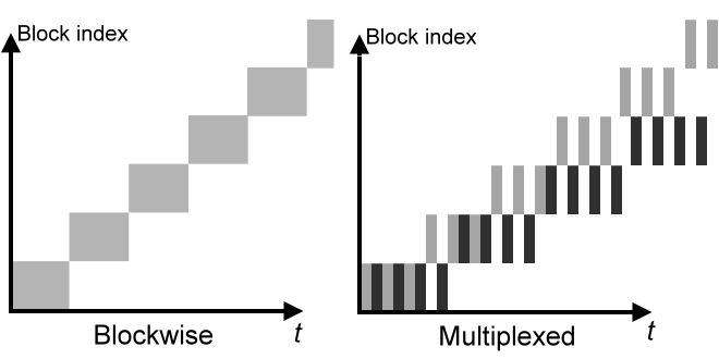
To suit the need of different receivers, we can perform time multiplexing on two blockwise codes at different rates. Cosider Blockwise code 1 and Blockwise code 2, which use random linear projections to encode each block of K𝐾K packets into L1subscript𝐿1L_{1} and L2subscript𝐿2L_{2} packets respectively (L1<L2subscript𝐿1subscript𝐿2L_{1}<L_{2}). Denote the i𝑖i-th packet generated using Blockwise code kπ‘˜k by Pk,isubscriptπ‘ƒπ‘˜π‘–P_{k,i}. We transmit the packets of the two codes in an interleaved manner (in the sequence P1,1,P2,1,P1,2,P2,2,P1,3,…subscript𝑃11subscript𝑃21subscript𝑃12subscript𝑃22subscript𝑃13…P_{1,1},P_{2,1},P_{1,2},P_{2,2},P_{1,3},...). Receiver 1, which uses only the packets generated using Blockwise code 1, can decode a block using K𝐾K out of the L1subscript𝐿1L_{1} packets encoded from the block, and therefore can tolerate a packet loss probability 1βˆ’K/L11𝐾subscript𝐿11-K/L_{1}. As Blockwise code 1 transmits a block of K𝐾K packet per L1subscript𝐿1L_{1} channel uses, taking interleaving into account, Receiver 1 can decode at a rate of K/(2​L1)𝐾2subscript𝐿1K/(2L_{1}) packets per channel use. Receiver 2 uses packets generated by both codes. It can decode a block using K𝐾K out of the L1+L2subscript𝐿1subscript𝐿2L_{1}+L_{2} packets encoded from the block, and allows a higher packet loss probability 1βˆ’K/(L1+L2)1𝐾subscript𝐿1subscript𝐿21-K/(L_{1}+L_{2}). However, to use the packets generated by both codes, Receiver 2 has to wait for the slower Blockwise code 2, which transmits a block of K𝐾K packet per L2subscript𝐿2L_{2} channel uses. Receiver 2 can decode at a rate K/(2​L2)𝐾2subscript𝐿2K/(2L_{2}).

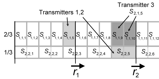
Refer to caption
Figure 1.1. Encoding process of blockwise and multiplexed codes

In the scenario, the receivers with different channel conditions wish to decode the same sequence of data. Each receiver will decode the data sequentially at a roughly constant rate which depends on the channel condition. We call these settings as multi-rate sequential data transmission. It can be viewed as multilevel diversity coding [1] with an additional sequential decoding constraint. In the following sections, we will discuss various cases of the problem. The case of one transmitter is described in Section 3. The main contribution lies in Section 6 concerning multiple transmitters, in which multi-rate sequential data transmission has apparently dissimilar behavior compared to its non-sequential counterpart.

2. Formulation of Multi-rate Sequential Data Transmission

We consider the transmission of a sequence of data through an erasure channel. To simplify the setting, we assume that one bit is sent at a time through the erasure channel. Assume the sender is going to transmit a sequence of bits M1,M2,…subscript𝑀1subscript𝑀2…M_{1},M_{2},.... We assume Mi∼i.i.d.Bern​(1/2)M_{i}\stackrel{{\scriptstyle i.i.d.}}{{\sim}}\mathrm{Bern}(1/2). The sender will encode it into a sequence of bits X1,X2,…subscript𝑋1subscript𝑋2…X_{1},X_{2},... and transmit them through an erasure channel. The symbols arrive at the receiver as Y1,Y2,…subscriptπ‘Œ1subscriptπ‘Œ2…Y_{1},Y_{2},..., where some of them may be erased (denoted by e𝑒e, Yi∈{0,1,e}subscriptπ‘Œπ‘–01𝑒Y_{i}\in\{0,1,e\}). Based on these symbols, the receiver tries to decode M1,M2,…subscript𝑀1subscript𝑀2…M_{1},M_{2},....

Definition 1 (MRS code).

A multi-rate sequential code (MRS code) is specified by a pair of encoding and decoding functions. The encoding function is a function mapping the message {Mi}subscript𝑀𝑖\left\{M_{i}\right\} to the encoding symbols {Xj}subscript𝑋𝑗\left\{X_{j}\right\}. There is a random variable Q𝑄Q supported in 𝒬𝒬\mathcal{Q} which is known by both the sender and the receiver, and independent of the message and the channel erasure, to allow random coding scheme. The encoding function is a function

Enc:𝒬×{0,1}β„•Γ—β„•:Enc𝒬superscript01β„•β„•\displaystyle\mathrm{Enc}\,:\,\mathcal{Q}\times\{0,1\}^{\mathbb{N}}\times\mathbb{N} β†’β†’\displaystyle\rightarrow {0,1}01\displaystyle\{0,1\}
(Q,{Mi},j)𝑄subscript𝑀𝑖𝑗\displaystyle\left(Q,\left\{M_{i}\right\},j\right) ↦maps-to\displaystyle\mapsto Xj.subscript𝑋𝑗\displaystyle X_{j}.

Note that this definition allows the encoder to look at all blocks.

The decoding function maps the received symbols {Yj}subscriptπ‘Œπ‘—\left\{Y_{j}\right\}, where some of them may be erased, to the recovered blocks {M~i}subscript~𝑀𝑖\left\{\widetilde{M}_{i}\right\}. Let 𝒴=⋃nβˆˆβ„•{0,1,e}n𝒴subscript𝑛ℕsuperscript01𝑒𝑛\mathcal{Y}=\bigcup_{n\in\mathbb{N}}\{0,1,e\}^{n} be the space of received symbols. The decoding function is a function

Dec:𝒬×𝒴×ℕ:Dec𝒬𝒴ℕ\displaystyle\mathrm{Dec}\,:\,\mathcal{Q}\times\mathcal{Y}\times\mathbb{N} β†’β†’\displaystyle\rightarrow {0,1}01\displaystyle\{0,1\}
(Q,Y1n,i)𝑄superscriptsubscriptπ‘Œ1𝑛𝑖\displaystyle\left(Q,Y_{1}^{n},i\right) ↦maps-to\displaystyle\mapsto M~i.subscript~𝑀𝑖\displaystyle\widetilde{M}_{i}.

We use the notation Yab=(Ya,Ya+1,…,Yb)superscriptsubscriptπ‘Œπ‘Žπ‘subscriptπ‘Œπ‘Žsubscriptπ‘Œπ‘Ž1…subscriptπ‘Œπ‘Y_{a}^{b}=(Y_{a},Y_{a+1},...,Y_{b}). For simplicity, we write Xj(Q,{Mi}))=Enc(Q,{Mi},j)X_{j}\left(Q,\left\{M_{i}\right\}\right))=\mathrm{Enc}\left(Q,\left\{M_{i}\right\},j\right), and M~i​(Q,Y1n)=Dec​(Q,Y1n,i)subscript~𝑀𝑖𝑄superscriptsubscriptπ‘Œ1𝑛Dec𝑄superscriptsubscriptπ‘Œ1𝑛𝑖\widetilde{M}_{i}\left(Q,Y_{1}^{n}\right)=\mathrm{Dec}\left(Q,Y_{1}^{n},i\right).

The MRS code does not admit a fixed rate like other block codes. Instead its rate depends on the channel capacity.

Definition 2 (admissible pair).

A rate-capacity pair (r,c)π‘Ÿπ‘(r,c) is called Ο΅italic-Ο΅\epsilon-admissible by a code if there exist N0subscript𝑁0N_{0} such that when Xiβ†’Yiβ†’subscript𝑋𝑖subscriptπ‘Œπ‘–X_{i}\to Y_{i} is an erasure channel with capacity c𝑐c (i.e. erasure channel with erasure probability 1βˆ’c1𝑐1-c),

ℙ​{Mmβ‰ M~m​(Q,Y1N)}≀ϡ​ for any ​Nβ‰₯N0​ and ​m≀N​(rβˆ’Ο΅).β„™subscriptπ‘€π‘šsubscript~π‘€π‘šπ‘„superscriptsubscriptπ‘Œ1𝑁italic-ϡ for any 𝑁subscript𝑁0Β andΒ π‘šπ‘π‘Ÿitalic-Ο΅\mathbb{P}\left\{M_{m}\neq\widetilde{M}_{m}\left(Q,Y_{1}^{N}\right)\right\}\leq\epsilon\>\text{ for any }N\geq N_{0}\text{ and }m\leq N(r-\epsilon).

In other words, any receiver with channel capacity c𝑐c can decode the first N​(rβˆ’Ο΅)π‘π‘Ÿitalic-Ο΅N(r-\epsilon) bits M1N​(rβˆ’Ο΅)superscriptsubscript𝑀1π‘π‘Ÿitalic-Ο΅M_{1}^{N(r-\epsilon)} with bit error probability less than Ο΅italic-Ο΅\epsilon when the first N𝑁N symbols Y1Nsuperscriptsubscriptπ‘Œ1𝑁Y_{1}^{N} are received, for sufficiently large N𝑁N.

It is clear that if (c,r)π‘π‘Ÿ(c,r) is Ο΅italic-Ο΅\epsilon-admissible, then all pairs in {(cβ€²,rβ€²)|cβ€²β‰₯c,r′≀r}conditional-setsuperscript𝑐′superscriptπ‘Ÿβ€²formulae-sequencesuperscript𝑐′𝑐superscriptπ‘Ÿβ€²π‘Ÿ\left\{(c^{\prime},r^{\prime})|c^{\prime}\geq c,r^{\prime}\leq r\right\} are Ο΅italic-Ο΅\epsilon-admissible. Therefore we can use a function to characterize the rate of a code. We call r:[0,1]β†’[0,∞):π‘Ÿβ†’010r:[0,1]\to[0,\infty) a rate-capacity function if it is monotonically increasing, right continuous, and there exists an Ξ·>0πœ‚0\eta>0 such that r​(c)=0π‘Ÿπ‘0r(c)=0 for cβ‰€Ξ·π‘πœ‚c\leq\eta.

Definition 3 (rate of MRS code).

A rate-capacity function r​(c)π‘Ÿπ‘r(c) is called Ο΅italic-Ο΅\epsilon-admissible by a code if all of the pairs (c,r​(c))π‘π‘Ÿπ‘(c,r(c)) are Ο΅italic-Ο΅\epsilon-admissible by the code.

The rate-capacity functions of the blockwise code and the multiplexed blockwise code described in the introduction can be given by Figure 2.1.
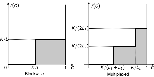
Refer to caption
Figure 2.1. Rate-capacity functions of blockwise and multiplexed blockwise code
Definition 4 (achievable rate-capacity functions).

A rate-capacity function r​(c)π‘Ÿπ‘r(c) is achievable if for any Ο΅>0italic-Ο΅0\epsilon>0, there exist a code where r​(c)π‘Ÿπ‘r(c) is Ο΅βˆ’limit-fromitalic-Ο΅\epsilon-admissible by that code.

3. Superposition Coding for Single Transmitter

In this section, we will present the design of superposition multi-rate sequential codes, and prove their optimality by giving the set of achievable rate-capacity functions explicitly.

Definition 5 (superposition MRS code).

A superposition MRS code is characterized by the block size K𝐾K and the parameter g:[0,∞)β†’[0,∞):𝑔→00g:[0,\infty)\to[0,\infty) which is bounded, monotonically decreasing and left continuous with ∫0∞g​(Ξ±)​𝑑α=1superscriptsubscript0𝑔𝛼differential-d𝛼1\int_{0}^{\infty}g(\alpha)d\alpha=1. The message {Mi}subscript𝑀𝑖\left\{M_{i}\right\} is divided into blocks of K𝐾K bits, Bi=M(iβˆ’1)​K+1i​Ksubscript𝐡𝑖superscriptsubscript𝑀𝑖1𝐾1𝑖𝐾B_{i}=M_{(i-1)K+1}^{iK}. In the encoding process of the code, we first sample a sequence of non-negative random variables A1,A2,…subscript𝐴1subscript𝐴2…A_{1},A_{2},... i.i.d. according to the cumulative distribution function

(3.1) FA​(Ξ±)subscript𝐹𝐴𝛼\displaystyle F_{A}(\alpha) =\displaystyle= ∫0Ξ±g​(x)​𝑑xβˆ’Ξ±β€‹g​(Ξ±)superscriptsubscript0𝛼𝑔π‘₯differential-dπ‘₯𝛼𝑔𝛼\displaystyle\int_{0}^{\alpha}g(x)dx-\alpha g(\alpha)
=\displaystyle= βˆ’βˆ«0Ξ±x​𝑑g​(x).superscriptsubscript0𝛼π‘₯differential-d𝑔π‘₯\displaystyle-\int_{0}^{\alpha}xdg(x).

Note that FA​(Ξ±)subscript𝐹𝐴𝛼F_{A}(\alpha) is increasing as g​(Ξ±)𝑔𝛼g(\alpha) is decreasing. The sequence is known by both the sender and the receiver (we may let Q=(A1,A2,…)𝑄subscript𝐴1subscript𝐴2…Q=(A_{1},A_{2},...)). At time instance i𝑖i, the sender generate an encoding symbol Xisubscript𝑋𝑖X_{i} from the block B⌈iβ‹…Ai/KβŒ‰subscript𝐡⋅𝑖subscript𝐴𝑖𝐾B_{\left\lceil i\cdot A_{i}/K\right\rceil} using random linear projections and transmit it to the receiver.

Note that we employ a random coding scheme. Random linear projections allow us to decode a block of K𝐾K bits using K+o​(K)πΎπ‘œπΎK+o(K) encoding bits with an arbitrarily small error probability. The superposition MRS code is essentially performing time multiplex on blockwise codes at different rates.

The parameter g​(Ξ±)𝑔𝛼g(\alpha) roughly corresponds to the proportion of the encoding symbols dedicated to satisfying the need of the receivers which wish to decode at rate α𝛼\alpha. When we send encoding symbols encoded at rate γ𝛾\gamma (i.e. Ai=Ξ³subscript𝐴𝑖𝛾A_{i}=\gamma), a receiver which decodes at rate α≀γ𝛼𝛾\alpha\leq\gamma can use a portion of Ξ±/γ𝛼𝛾\alpha/\gamma of the encoding symbols. The parameter g​(Ξ±)𝑔𝛼g(\alpha) describes the proportion of the symbols which can be used, divided by the proportion needed (which is α𝛼\alpha), given by

g​(Ξ±)=1Ξ±β€‹βˆ«Ξ±βˆžΞ±Ξ³β€‹π‘‘FA​(Ξ³),𝑔𝛼1𝛼superscriptsubscript𝛼𝛼𝛾differential-dsubscript𝐹𝐴𝛾g(\alpha)=\frac{1}{\alpha}\int_{\alpha}^{\infty}\frac{\alpha}{\gamma}dF_{A}(\gamma),

which can be verified using (3.1):

1Ξ±β€‹βˆ«Ξ±βˆžΞ±Ξ³β€‹π‘‘FA​(Ξ³)1𝛼superscriptsubscript𝛼𝛼𝛾differential-dsubscript𝐹𝐴𝛾\displaystyle\frac{1}{\alpha}\int_{\alpha}^{\infty}\frac{\alpha}{\gamma}dF_{A}(\gamma) =\displaystyle= ∫α∞1γ​𝑑FA​(Ξ³)superscriptsubscript𝛼1𝛾differential-dsubscript𝐹𝐴𝛾\displaystyle\int_{\alpha}^{\infty}\frac{1}{\gamma}dF_{A}(\gamma)
=\displaystyle= βˆ’βˆ«Ξ±βˆž1γ⋅γ​𝑑g​(Ξ³)superscriptsubscript𝛼⋅1𝛾𝛾differential-d𝑔𝛾\displaystyle-\int_{\alpha}^{\infty}\frac{1}{\gamma}\cdot\gamma dg(\gamma)
=\displaystyle= βˆ’βˆ«Ξ±βˆžπ‘‘g​(Ξ³)=g​(Ξ±).superscriptsubscript𝛼differential-d𝑔𝛾𝑔𝛼\displaystyle-\int_{\alpha}^{\infty}dg(\gamma)=g(\alpha).

The blockwise code and the multiplexed blockwise code described in the introduction are examples of superposition MRS codes. For the blockwise code, the parameter is taken to be

g​(Ξ±)={L/KΒ when ​α≀K/L0Β when ​α>K/L.𝑔𝛼cases𝐿𝐾 when 𝛼𝐾𝐿0Β when 𝛼𝐾𝐿g(\alpha)=\begin{cases}L/K&\text{ when }\alpha\leq K/L\\ 0&\text{ when }\alpha>K/L.\end{cases}

For the multiplexed blockwise code, the parameter is taken to be

g​(Ξ±)={L1+L2KΒ when ​α≀K2​L2L1KΒ when ​K2​L2<α≀K2​L10Β when ​α>K2​L1.𝑔𝛼casessubscript𝐿1subscript𝐿2𝐾 when 𝛼𝐾2subscript𝐿2subscript𝐿1𝐾 when 𝐾2subscript𝐿2𝛼𝐾2subscript𝐿10Β when 𝛼𝐾2subscript𝐿1g(\alpha)=\begin{cases}\frac{L_{1}+L_{2}}{K}&\text{ when }\alpha\leq\frac{K}{2L_{2}}\\ \frac{L_{1}}{K}&\text{ when }\frac{K}{2L_{2}}<\alpha\leq\frac{K}{2L_{1}}\\ 0&\text{ when }\alpha>\frac{K}{2L_{1}}.\end{cases}

The choice of the parameter is closely related to the rate-capacity function we would like to achieve. The following theorem describes the relationship between the two functions.

Theorem 6.

For a fixed Ο΅italic-Ο΅\epsilon, the rate-capacity function r​(c)π‘Ÿπ‘r(c) is Ο΅italic-Ο΅\epsilon-admissible by the superposition MRS code with block size K𝐾K and parameter g​(Ξ±)𝑔𝛼g(\alpha) for all sufficiently large K𝐾K, if there exists ΞΎ>0πœ‰0\xi>0 satisfying

cβ‹…g​(r​(c))β‰₯1+ξ​ for all ​c>0​ with ​r​(c)>0.β‹…π‘π‘”π‘Ÿπ‘1πœ‰Β for all 𝑐0Β withΒ π‘Ÿπ‘0c\cdot g\left(r(c)\right)\geq 1+\xi\text{ for all }c>0\text{ with }r(c)>0.
Proof.

Fix Ο΅>0italic-Ο΅0\epsilon>0. Let r​(c)π‘Ÿπ‘r(c) be a rate-capacity function, and let g​(Ξ±)𝑔𝛼g(\alpha) be a bounded and monotonically decreasing function (let g​(Ξ±)β‰€ΞΆπ‘”π›Όπœg(\alpha)\leq\zeta for all Ξ±β‰₯0𝛼0\alpha\geq 0). Assume the condition cβ‹…g​(r​(c))β‰₯1+ΞΎβ‹…π‘π‘”π‘Ÿπ‘1πœ‰c\cdot g\left(r(c)\right)\geq 1+\xi is satisfied for some ΞΎ>0πœ‰0\xi>0. We take Kβ‰₯max⁑(4/ΞΎ, 32β‹…(ΞΆ+1)/(ϡ​ξ))𝐾4πœ‰β‹…32𝜁1italic-Ο΅πœ‰K\geq\max\left(4/\xi,\,32\cdot(\zeta+1)/(\epsilon\xi)\right). We now consider the superposition MRS code with block size K𝐾K and parameter g​(Ξ±)𝑔𝛼g(\alpha).

Fix any channel capacity c𝑐c with r​(c)>0π‘Ÿπ‘0r(c)>0. Let Ξ±1=r​(c)subscript𝛼1π‘Ÿπ‘\alpha_{1}=r(c), and Ξ±0=r​(c)βˆ’Ο΅subscript𝛼0π‘Ÿπ‘italic-Ο΅\alpha_{0}=r(c)-\epsilon. At time instance i𝑖i, the sender generate an encoding symbol from the block B⌈iβ‹…Ai/KβŒ‰subscript𝐡⋅𝑖subscript𝐴𝑖𝐾B_{\left\lceil i\cdot A_{i}/K\right\rceil} (note that Bi=M(iβˆ’1)​K+1i​Ksubscript𝐡𝑖superscriptsubscript𝑀𝑖1𝐾1𝑖𝐾B_{i}=M_{(i-1)K+1}^{iK}). Let FA​(Ξ±)=∫0Ξ±g​(x)​𝑑xβˆ’Ξ±β€‹g​(Ξ±)subscript𝐹𝐴𝛼superscriptsubscript0𝛼𝑔π‘₯differential-dπ‘₯𝛼𝑔𝛼F_{A}(\alpha)=\int_{0}^{\alpha}g(x)dx-\alpha g(\alpha). The probability that Bjsubscript𝐡𝑗B_{j} is chosen is

ℙ​{Ai∈(K​(jβˆ’1)i,K​ji]}=FA​(K​ji)βˆ’FA​(K​(jβˆ’1)i).β„™subscript𝐴𝑖𝐾𝑗1𝑖𝐾𝑗𝑖subscript𝐹𝐴𝐾𝑗𝑖subscript𝐹𝐴𝐾𝑗1𝑖\mathbb{P}\left\{A_{i}\in\left(\frac{K(j-1)}{i},\frac{Kj}{i}\right]\right\}=F_{A}\left(\frac{Kj}{i}\right)-F_{A}\left(\frac{K(j-1)}{i}\right).

Let nβ‰₯Kϡ𝑛𝐾italic-Ο΅n\geq\frac{K}{\epsilon}, and j≀n​α0K+1𝑗𝑛subscript𝛼0𝐾1j\leq\frac{n\alpha_{0}}{K}+1. We will study whether the block Bjsubscript𝐡𝑗B_{j} can be decoded using Y1nsuperscriptsubscriptπ‘Œ1𝑛Y_{1}^{n} with error probability less than Ο΅italic-Ο΅\epsilon when the channel capacity is c𝑐c. If so, then M1⌊α0​nβŒ‹superscriptsubscript𝑀1subscript𝛼0𝑛M_{1}^{\left\lfloor\alpha_{0}n\right\rfloor} can be decoded using Y1nsuperscriptsubscriptπ‘Œ1𝑛Y_{1}^{n} with bit error probability less than Ο΅italic-Ο΅\epsilon whenever nβ‰₯Kϡ𝑛𝐾italic-Ο΅n\geq\frac{K}{\epsilon}, and thus the rate-capacity pair (Ξ±1,c)subscript𝛼1𝑐(\alpha_{1},c) is Ο΅βˆ’limit-fromitalic-Ο΅\epsilon-admissible. Let S𝑆S be the random variable representing the number of times Bjsubscript𝐡𝑗B_{j} is chosen in the encoding of Xisubscript𝑋𝑖X_{i}, and Xisubscript𝑋𝑖X_{i} is not erased, for i=1,…,n𝑖1…𝑛i=1,...,n. Its expected value is given by

𝔼​[S]𝔼delimited-[]𝑆\displaystyle\mathbb{E}[S] =\displaystyle= cβ‹…βˆ‘i=1n(FA​(K​ji)βˆ’FA​(K​(jβˆ’1)i)).⋅𝑐superscriptsubscript𝑖1𝑛subscript𝐹𝐴𝐾𝑗𝑖subscript𝐹𝐴𝐾𝑗1𝑖\displaystyle c\cdot\sum_{i=1}^{n}\left(F_{A}\left(\frac{Kj}{i}\right)-F_{A}\left(\frac{K(j-1)}{i}\right)\right).

Note that FAsubscript𝐹𝐴F_{A} is monotonically increasing and not greater than 1 (and therefore FA​(K​jn​x)subscript𝐹𝐴𝐾𝑗𝑛π‘₯F_{A}\left(\frac{Kj}{nx}\right) is monotonically decreasing with respect to xπ‘₯x), we have

βˆ‘i=1nFA​(K​ji)superscriptsubscript𝑖1𝑛subscript𝐹𝐴𝐾𝑗𝑖\displaystyle\sum_{i=1}^{n}F_{A}\left(\frac{Kj}{i}\right) β‰₯\displaystyle\geq n​(∫1/n1FA​(K​jn​x)​𝑑x)𝑛superscriptsubscript1𝑛1subscript𝐹𝐴𝐾𝑗𝑛π‘₯differential-dπ‘₯\displaystyle n\left(\int_{1/n}^{1}F_{A}\left(\frac{Kj}{nx}\right)dx\right)
β‰₯\displaystyle\geq n​(∫01FA​(K​jn​x)​𝑑x)βˆ’1,𝑛superscriptsubscript01subscript𝐹𝐴𝐾𝑗𝑛π‘₯differential-dπ‘₯1\displaystyle n\left(\int_{0}^{1}F_{A}\left(\frac{Kj}{nx}\right)dx\right)-1,
βˆ‘i=1nFA​(K​(jβˆ’1)i)superscriptsubscript𝑖1𝑛subscript𝐹𝐴𝐾𝑗1𝑖\displaystyle\sum_{i=1}^{n}F_{A}\left(\frac{K(j-1)}{i}\right) ≀\displaystyle\leq n​(∫01FA​(K​(jβˆ’1)n​x)​𝑑x).𝑛superscriptsubscript01subscript𝐹𝐴𝐾𝑗1𝑛π‘₯differential-dπ‘₯\displaystyle n\left(\int_{0}^{1}F_{A}\left(\frac{K(j-1)}{nx}\right)dx\right).

Therefore

𝔼​[S]𝔼delimited-[]𝑆\displaystyle\mathbb{E}[S] β‰₯\displaystyle\geq c​n​(∫01(FA​(K​jn​x)βˆ’FA​(K​(jβˆ’1)n​x))​𝑑x)βˆ’c𝑐𝑛superscriptsubscript01subscript𝐹𝐴𝐾𝑗𝑛π‘₯subscript𝐹𝐴𝐾𝑗1𝑛π‘₯differential-dπ‘₯𝑐\displaystyle cn\left(\int_{0}^{1}\left(F_{A}\left(\frac{Kj}{nx}\right)-F_{A}\left(\frac{K(j-1)}{nx}\right)\right)dx\right)-c
β‰₯\displaystyle\geq c​n​(∫01(FA​(K​jn​x)βˆ’FA​(K​(jβˆ’1)n​x))​𝑑x)βˆ’1,𝑐𝑛superscriptsubscript01subscript𝐹𝐴𝐾𝑗𝑛π‘₯subscript𝐹𝐴𝐾𝑗1𝑛π‘₯differential-dπ‘₯1\displaystyle cn\left(\int_{0}^{1}\left(F_{A}\left(\frac{Kj}{nx}\right)-F_{A}\left(\frac{K(j-1)}{nx}\right)\right)dx\right)-1,

where

∫01FA​(Ξ±x)​𝑑xsuperscriptsubscript01subscript𝐹𝐴𝛼π‘₯differential-dπ‘₯\displaystyle\int_{0}^{1}F_{A}\left(\frac{\alpha}{x}\right)dx =\displaystyle= FA​(Ξ±)βˆ’βˆ«01x​𝑑FA​(Ξ±x)subscript𝐹𝐴𝛼superscriptsubscript01π‘₯differential-dsubscript𝐹𝐴𝛼π‘₯\displaystyle F_{A}(\alpha)-\int_{0}^{1}xdF_{A}\left(\frac{\alpha}{x}\right)
=\displaystyle= FA​(Ξ±)+Ξ±β€‹βˆ«Ξ±βˆž1x​𝑑FA​(x)subscript𝐹𝐴𝛼𝛼superscriptsubscript𝛼1π‘₯differential-dsubscript𝐹𝐴π‘₯\displaystyle F_{A}(\alpha)+\alpha\int_{\alpha}^{\infty}\frac{1}{x}dF_{A}\left(x\right)
=\displaystyle= FA(Ξ±)+α∫α∞1xβ‹…βˆ’xdg(x)\displaystyle F_{A}(\alpha)+\alpha\int_{\alpha}^{\infty}\frac{1}{x}\cdot-xdg(x)
=\displaystyle= FA​(Ξ±)βˆ’Ξ±β€‹βˆ«Ξ±βˆž1​𝑑g​(x)subscript𝐹𝐴𝛼𝛼superscriptsubscript𝛼1differential-d𝑔π‘₯\displaystyle F_{A}(\alpha)-\alpha\int_{\alpha}^{\infty}1dg(x)
=\displaystyle= FA​(Ξ±)+α​g​(Ξ±)subscript𝐹𝐴𝛼𝛼𝑔𝛼\displaystyle F_{A}(\alpha)+\alpha g(\alpha)
=\displaystyle= ∫0Ξ±g​(x)​𝑑x.superscriptsubscript0𝛼𝑔π‘₯differential-dπ‘₯\displaystyle\int_{0}^{\alpha}g(x)dx.

Hence, as g​(x)𝑔π‘₯g(x) is monotonically decreasing,

𝔼​[S]𝔼delimited-[]𝑆\displaystyle\mathbb{E}[S] β‰₯\displaystyle\geq c​nβ‹…(∫0K​j/ng​(x)​𝑑xβˆ’βˆ«0K​(jβˆ’1)/ng​(x)​𝑑x)βˆ’1⋅𝑐𝑛superscriptsubscript0𝐾𝑗𝑛𝑔π‘₯differential-dπ‘₯superscriptsubscript0𝐾𝑗1𝑛𝑔π‘₯differential-dπ‘₯1\displaystyle cn\cdot\left(\int_{0}^{Kj/n}g(x)dx-\int_{0}^{K(j-1)/n}g(x)dx\right)-1
=\displaystyle= c​nβ‹…βˆ«K​(jβˆ’1)/nK​j/ng​(x)​𝑑xβˆ’1⋅𝑐𝑛superscriptsubscript𝐾𝑗1𝑛𝐾𝑗𝑛𝑔π‘₯differential-dπ‘₯1\displaystyle cn\cdot\int_{K(j-1)/n}^{Kj/n}g(x)dx-1
β‰₯\displaystyle\geq c​Kβ‹…g​(K​jn)βˆ’1⋅𝑐𝐾𝑔𝐾𝑗𝑛1\displaystyle cK\cdot g\left(\frac{Kj}{n}\right)-1
β‰₯\displaystyle\geq c​Kβ‹…g​(Ξ±0+Kn)βˆ’1⋅𝑐𝐾𝑔subscript𝛼0𝐾𝑛1\displaystyle cK\cdot g\left(\alpha_{0}+\frac{K}{n}\right)-1
β‰₯\displaystyle\geq c​Kβ‹…g​(Ξ±0+Ο΅)βˆ’1⋅𝑐𝐾𝑔subscript𝛼0italic-Ο΅1\displaystyle cK\cdot g\left(\alpha_{0}+\epsilon\right)-1
=\displaystyle= c​Kβ‹…g​(Ξ±1)βˆ’1⋅𝑐𝐾𝑔subscript𝛼11\displaystyle cK\cdot g\left(\alpha_{1}\right)-1
β‰₯\displaystyle\geq K​(1+ΞΎ)βˆ’1.𝐾1πœ‰1\displaystyle K(1+\xi)-1.

On the other hand,

βˆ‘i=1nFA​(K​ji)superscriptsubscript𝑖1𝑛subscript𝐹𝐴𝐾𝑗𝑖\displaystyle\sum_{i=1}^{n}F_{A}\left(\frac{Kj}{i}\right) ≀\displaystyle\leq n​(∫01FA​(K​jn​x)​𝑑x),𝑛superscriptsubscript01subscript𝐹𝐴𝐾𝑗𝑛π‘₯differential-dπ‘₯\displaystyle n\left(\int_{0}^{1}F_{A}\left(\frac{Kj}{nx}\right)dx\right),

and

βˆ‘i=1nFA​(K​(jβˆ’1)i)superscriptsubscript𝑖1𝑛subscript𝐹𝐴𝐾𝑗1𝑖\displaystyle\sum_{i=1}^{n}F_{A}\left(\frac{K(j-1)}{i}\right) β‰₯\displaystyle\geq n​(∫1/n1FA​(K​(jβˆ’1)n​x)​𝑑x)𝑛superscriptsubscript1𝑛1subscript𝐹𝐴𝐾𝑗1𝑛π‘₯differential-dπ‘₯\displaystyle n\left(\int_{1/n}^{1}F_{A}\left(\frac{K(j-1)}{nx}\right)dx\right)
β‰₯\displaystyle\geq n​(∫01FA​(K​(jβˆ’1)n​x)​𝑑x)βˆ’1.𝑛superscriptsubscript01subscript𝐹𝐴𝐾𝑗1𝑛π‘₯differential-dπ‘₯1\displaystyle n\left(\int_{0}^{1}F_{A}\left(\frac{K(j-1)}{nx}\right)dx\right)-1.

Let

pi=c​(FA​(K​ji)βˆ’FA​(K​(jβˆ’1)i)).subscript𝑝𝑖𝑐subscript𝐹𝐴𝐾𝑗𝑖subscript𝐹𝐴𝐾𝑗1𝑖p_{i}=c\left(F_{A}\left(\frac{Kj}{i}\right)-F_{A}\left(\frac{K(j-1)}{i}\right)\right).

The variance of S𝑆S can be given by

Var​[S]Vardelimited-[]𝑆\displaystyle\mathrm{Var}[S] =\displaystyle= βˆ‘i=1n(piβˆ’pi2)superscriptsubscript𝑖1𝑛subscript𝑝𝑖superscriptsubscript𝑝𝑖2\displaystyle\sum_{i=1}^{n}\left(p_{i}-p_{i}^{2}\right)
≀\displaystyle\leq βˆ‘i=1npisuperscriptsubscript𝑖1𝑛subscript𝑝𝑖\displaystyle\sum_{i=1}^{n}p_{i}
≀\displaystyle\leq c​nβ‹…(∫01(FA​(K​jn​x)βˆ’FA​(K​(jβˆ’1)n​x))​𝑑x)+c⋅𝑐𝑛superscriptsubscript01subscript𝐹𝐴𝐾𝑗𝑛π‘₯subscript𝐹𝐴𝐾𝑗1𝑛π‘₯differential-dπ‘₯𝑐\displaystyle cn\cdot\left(\int_{0}^{1}\left(F_{A}\left(\frac{Kj}{nx}\right)-F_{A}\left(\frac{K(j-1)}{nx}\right)\right)dx\right)+c
≀\displaystyle\leq nβ‹…(∫01(FA​(K​jn​x)βˆ’FA​(K​(jβˆ’1)n​x))​𝑑x)+1⋅𝑛superscriptsubscript01subscript𝐹𝐴𝐾𝑗𝑛π‘₯subscript𝐹𝐴𝐾𝑗1𝑛π‘₯differential-dπ‘₯1\displaystyle n\cdot\left(\int_{0}^{1}\left(F_{A}\left(\frac{Kj}{nx}\right)-F_{A}\left(\frac{K(j-1)}{nx}\right)\right)dx\right)+1
=\displaystyle= nβ‹…(∫0K​j/ng2​(x)​𝑑xβˆ’βˆ«0K​(jβˆ’1)/ng2​(x)​𝑑x)+1⋅𝑛superscriptsubscript0𝐾𝑗𝑛subscript𝑔2π‘₯differential-dπ‘₯superscriptsubscript0𝐾𝑗1𝑛subscript𝑔2π‘₯differential-dπ‘₯1\displaystyle n\cdot\left(\int_{0}^{Kj/n}g_{2}(x)dx-\int_{0}^{K(j-1)/n}g_{2}(x)dx\right)+1
=\displaystyle= nβ‹…βˆ«K​(jβˆ’1)/nK​j/ng2​(x)​𝑑x+1⋅𝑛superscriptsubscript𝐾𝑗1𝑛𝐾𝑗𝑛subscript𝑔2π‘₯differential-dπ‘₯1\displaystyle n\cdot\int_{K(j-1)/n}^{Kj/n}g_{2}(x)dx+1
≀\displaystyle\leq K​΢+1,𝐾𝜁1\displaystyle K\zeta+1,
ΟƒS≀Kβ‹…ΞΆ+1.subscriptπœŽπ‘†β‹…πΎπœ1\sigma_{S}\leq\sqrt{K}\cdot\sqrt{\zeta+1}.

As a result, for K𝐾K large enough, S𝑆S is close to 𝔼​[S]𝔼delimited-[]𝑆\mathbb{E}[S] with high probability. Chebyshev’s inequality gives

ℙ​{S<K​(1+ΞΎ)βˆ’1βˆ’Kβ‹…ΞΆ+1Ο΅/2}≀ϡ/2,ℙ𝑆𝐾1πœ‰1β‹…πΎπœ1italic-Ο΅2italic-Ο΅2\mathbb{P}\left\{S<K(1+\xi)-1-\frac{\sqrt{K}\cdot\sqrt{\zeta+1}}{\sqrt{\epsilon/2}}\right\}\leq\epsilon/2,

where

K​(1+ΞΎ)βˆ’1βˆ’Kβ‹…ΞΆ+1Ο΅/2𝐾1πœ‰1β‹…πΎπœ1italic-Ο΅2\displaystyle K(1+\xi)-1-\frac{\sqrt{K}\cdot\sqrt{\zeta+1}}{\sqrt{\epsilon/2}}
=\displaystyle= K​(1+ΞΎβˆ’1Kβˆ’ΞΆ+1K​ϡ/2)𝐾1πœ‰1𝐾𝜁1𝐾italic-Ο΅2\displaystyle K\left(1+\xi-\frac{1}{K}-\frac{\sqrt{\zeta+1}}{\sqrt{K\epsilon/2}}\right)
β‰₯\displaystyle\geq K​(1+ΞΎ/2)𝐾1πœ‰2\displaystyle K\left(1+\xi/2\right)

by the assumption Kβ‰₯max⁑(4/ΞΎ, 32β‹…(ΞΆ+1)/(ϡ​ξ))𝐾4πœ‰β‹…32𝜁1italic-Ο΅πœ‰K\geq\max\left(4/\xi,\,32\cdot(\zeta+1)/(\epsilon\xi)\right). When random linear projections are used, for a fixed probability of error Ο΅/2italic-Ο΅2\epsilon/2, the number of symbols needed to decode a block of K𝐾K bits is K+o​(K)πΎπ‘œπΎK+o(K), which is smaller than K​(1+ΞΎ/2)𝐾1πœ‰2K\left(1+\xi/2\right) for sufficiently large K𝐾K. Therefore the rate function r​(c)π‘Ÿπ‘r(c) is Ο΅italic-Ο΅\epsilon-admissable by the superposition MRS code with parameter g​(Ξ±)𝑔𝛼g(\alpha) for K𝐾K large enough. ∎

The following theorem gives the achievable region for the rate-capacity function, which coincides with the region attained by superposition MRS code.

Theorem 7.

A rate-capacity function r​(c)π‘Ÿπ‘r(c) is achievable if and only if

∫011c​𝑑r​(c)≀1.superscriptsubscript011𝑐differential-dπ‘Ÿπ‘1\int_{0}^{1}\frac{1}{c}dr(c)\leq 1.
Proof of achievability.

Assume r​(c)π‘Ÿπ‘r(c) is a rate-capacity function satisfying ∫011c​𝑑r​(c)≀1superscriptsubscript011𝑐differential-dπ‘Ÿπ‘1\int_{0}^{1}\frac{1}{c}dr(c)\leq 1. We can find Ξ·>0πœ‚0\eta>0 such that r​(c)=0π‘Ÿπ‘0r(c)=0 for cβ‰€Ξ·π‘πœ‚c\leq\eta. Let g​(Ξ±)=1/rβˆ’1​(Ξ±)𝑔𝛼1superscriptπ‘Ÿ1𝛼g(\alpha)=1/r^{-1}(\alpha), where rβˆ’1​(Ξ±)=inf{c|r​(c)β‰₯Ξ±}superscriptπ‘Ÿ1𝛼infimumconditional-setπ‘π‘Ÿπ‘π›Όr^{-1}(\alpha)=\inf\{c|r(c)\geq\alpha\}. Then g​(Ξ±)𝑔𝛼g(\alpha) is monotonically decreasing and bounded above by 1/Ξ·1πœ‚1/\eta. It is implied by ∫011c​𝑑r​(c)≀1superscriptsubscript011𝑐differential-dπ‘Ÿπ‘1\int_{0}^{1}\frac{1}{c}dr(c)\leq 1 that ∫0∞g​(Ξ±)​𝑑α≀1superscriptsubscript0𝑔𝛼differential-d𝛼1\int_{0}^{\infty}g(\alpha)d\alpha\leq 1. As rβˆ’1​(r​(c))≀csuperscriptπ‘Ÿ1π‘Ÿπ‘π‘r^{-1}(r(c))\leq c, we also have cβ‹…g​(r​(c))β‰₯1β‹…π‘π‘”π‘Ÿπ‘1c\cdot g\left(r(c)\right)\geq 1 for all c>0𝑐0c>0 with r​(c)>0π‘Ÿπ‘0r(c)>0.

Fix Ο΅>0italic-Ο΅0\epsilon>0. Note that ∫0∞g​(Ξ±+Ο΅/2)​𝑑α<1superscriptsubscript0𝑔𝛼italic-Ο΅2differential-d𝛼1\int_{0}^{\infty}g(\alpha+\epsilon/2)d\alpha<1. We can define a function g2​(Ξ±)subscript𝑔2𝛼g_{2}(\alpha) by

g2​(Ξ±)=(1+ΞΎ)β‹…g​(Ξ±+Ο΅/2),subscript𝑔2𝛼⋅1πœ‰π‘”π›Όitalic-Ο΅2g_{2}(\alpha)=(1+\xi)\cdot g(\alpha+\epsilon/2),

where ΞΎ>0πœ‰0\xi>0 such that ∫0∞g2​(Ξ±)​𝑑α=1superscriptsubscript0subscript𝑔2𝛼differential-d𝛼1\int_{0}^{\infty}g_{2}(\alpha)d\alpha=1. We know g2subscript𝑔2g_{2} is bounded above by (1+ΞΎ)/Ξ·1πœ‰πœ‚(1+\xi)/\eta. Define a new rate-capacity function r2​(c)=max⁑(r​(c)βˆ’Ο΅/2,0)subscriptπ‘Ÿ2π‘π‘Ÿπ‘italic-Ο΅20r_{2}(c)=\max(r(c)-\epsilon/2,0). We have, for any c𝑐c with r2​(c)>0subscriptπ‘Ÿ2𝑐0r_{2}(c)>0,

cβ‹…g2​(r2​(c))=cβ‹…(1+ΞΎ)​g​(r​(c))β‰₯1+ΞΎ.⋅𝑐subscript𝑔2subscriptπ‘Ÿ2𝑐⋅𝑐1πœ‰π‘”π‘Ÿπ‘1πœ‰c\cdot g_{2}\left(r_{2}(c)\right)=c\cdot(1+\xi)g\left(r(c)\right)\geq 1+\xi.

Consider the superposition MRS code with parameter g2​(Ξ±)subscript𝑔2𝛼g_{2}(\alpha). By Theorem 6, the rate-capacity function r2​(c)subscriptπ‘Ÿ2𝑐r_{2}(c) is Ο΅/2italic-Ο΅2\epsilon/2-admissible by the code for sufficiently large block size, which implies that r​(c)π‘Ÿπ‘r(c) is Ο΅italic-Ο΅\epsilon-admissible by the code. ∎

 
Proof of converse.

The proof employs a similar idea as in [2]. As r​(c)π‘Ÿπ‘r(c) is a rate-capacity function, we can find Ξ·>0πœ‚0\eta>0 such that r​(c)=0π‘Ÿπ‘0r(c)=0 for cβ‰€Ξ·π‘πœ‚c\leq\eta. For any Ο΅>0italic-Ο΅0\epsilon>0, consider a code where r​(c)π‘Ÿπ‘r(c) is Ο΅italic-Ο΅\epsilon-admissible. The message {Mi}subscript𝑀𝑖\{M_{i}\} are encoded into binary symbols {Xi}subscript𝑋𝑖\{X_{i}\}, and sent through an erasure channel with capacity c𝑐c (we call it Channel c𝑐c) to give {Yc,i}subscriptπ‘Œπ‘π‘–\{Y_{c,i}\} for all c>0𝑐0c>0. Assume we have the following for any c𝑐c,

maxm≀n​(r​(c)βˆ’Ο΅)⁑ℙ​{Mmβ‰ M~m​(Q,Yc,1n)}<ϡ​ for any ​nβ‰₯N0.subscriptπ‘šπ‘›π‘Ÿπ‘italic-Ο΅β„™subscriptπ‘€π‘šsubscript~π‘€π‘šπ‘„superscriptsubscriptπ‘Œπ‘1𝑛italic-ϡ for any 𝑛subscript𝑁0\max_{m\leq n(r(c)-\epsilon)}\mathbb{P}\left\{M_{m}\neq\widetilde{M}_{m}\left(Q,Y_{c,1}^{n}\right)\right\}<\epsilon\>\text{ for any }n\geq N_{0}.

Let Nβ‰₯N0𝑁subscript𝑁0N\geq N_{0}. Let Ec,isubscript𝐸𝑐𝑖E_{c,i} be the indicator of the events of erasure in Channel c𝑐c (Ec,i=1subscript𝐸𝑐𝑖1E_{c,i}=1 means that Yc,i=esubscriptπ‘Œπ‘π‘–π‘’Y_{c,i}=e). Note that whether the message can be decoded at the receiver with Channel c𝑐c depends only on the marginal distribution of {Ec,i,Xi,Mi,Q}iβˆˆβ„•subscriptsubscript𝐸𝑐𝑖subscript𝑋𝑖subscript𝑀𝑖𝑄𝑖ℕ\left\{E_{c,i},X_{i},M_{i},Q\right\}_{i\in\mathbb{N}}, and is conditional independent of Ec2,isubscript𝐸subscript𝑐2𝑖E_{c_{2},i} for c2β‰ csubscript𝑐2𝑐c_{2}\neq c given {Ec,i,Xi,Mi,Q}iβˆˆβ„•subscriptsubscript𝐸𝑐𝑖subscript𝑋𝑖subscript𝑀𝑖𝑄𝑖ℕ\left\{E_{c,i},X_{i},M_{i},Q\right\}_{i\in\mathbb{N}}. Therefore, we may modify the joint distribution of {Ec,i}c∈(0,1],iβˆˆβ„•subscriptsubscript𝐸𝑐𝑖formulae-sequence𝑐01𝑖ℕ\left\{E_{c,i}\right\}_{c\in(0,1],i\in\mathbb{N}} without affecting the result as long as the distributions of {Ec,i,Xi,Mi,Q}iβˆˆβ„•subscriptsubscript𝐸𝑐𝑖subscript𝑋𝑖subscript𝑀𝑖𝑄𝑖ℕ\left\{E_{c,i},X_{i},M_{i},Q\right\}_{i\in\mathbb{N}} are preserved. From now on, we assume the channels are cascaded, i.e. whenever c0<c1≀1subscript𝑐0subscript𝑐11c_{0}<c_{1}\leq 1, the Markov chain Xiβ†’Yc1,iβ†’Yc0,iβ†’subscript𝑋𝑖subscriptπ‘Œsubscript𝑐1𝑖→subscriptπ‘Œsubscript𝑐0𝑖X_{i}\rightarrow Y_{c_{1},i}\rightarrow Y_{c_{0},i} holds, and

Ec0,i={Ec1,iΒ w.p. ​c0/c11Β w.p. ​1βˆ’c0/c1.subscript𝐸subscript𝑐0𝑖casessubscript𝐸subscript𝑐1𝑖 w.p.Β subscript𝑐0subscript𝑐11Β w.p.Β 1subscript𝑐0subscript𝑐1E_{c_{0},i}=\begin{cases}E_{c_{1},i}&\text{ w.p. }c_{0}/c_{1}\\ 1&\text{ w.p. }1-c_{0}/c_{1}.\end{cases}

Let

(3.2) r2​(c)=max⁑(r​(c)βˆ’Ο΅,0).subscriptπ‘Ÿ2π‘π‘Ÿπ‘italic-Ο΅0r_{2}(c)=\max(r(c)-\epsilon,0).

Define

(3.3) f​(c)=1N​cβ‹…H​(Yc,1N|Q,M1⌊N​r2​(c)βŒ‹,Ec,1N).𝑓𝑐⋅1𝑁𝑐𝐻conditionalsuperscriptsubscriptπ‘Œπ‘1𝑁𝑄superscriptsubscript𝑀1𝑁subscriptπ‘Ÿ2𝑐superscriptsubscript𝐸𝑐1𝑁f(c)=\frac{1}{Nc}\cdot H(Y_{c,1}^{N}|Q,M_{1}^{\left\lfloor Nr_{2}(c)\right\rfloor},E_{c,1}^{N}).

The common random variable Q𝑄Q will be omitted for simplicity. Consider Channel c0subscript𝑐0c_{0} and Channel c1subscript𝑐1c_{1} where Ξ·/2≀c0<c1≀1πœ‚2subscript𝑐0subscript𝑐11\eta/2\leq c_{0}<c_{1}\leq 1. Let k0=⌊N​r2​(c0)βŒ‹subscriptπ‘˜0𝑁subscriptπ‘Ÿ2subscript𝑐0k_{0}=\left\lfloor Nr_{2}(c_{0})\right\rfloor, and k1=⌊N​r2​(c1)βŒ‹subscriptπ‘˜1𝑁subscriptπ‘Ÿ2subscript𝑐1k_{1}=\left\lfloor Nr_{2}(c_{1})\right\rfloor. Note that

(3.4) H​(Yc1,1N|M1k1,Ec1,1N)𝐻conditionalsuperscriptsubscriptπ‘Œsubscript𝑐11𝑁superscriptsubscript𝑀1subscriptπ‘˜1superscriptsubscript𝐸subscript𝑐11𝑁\displaystyle H(Y_{c_{1},1}^{N}|M_{1}^{k_{1}},E_{c_{1},1}^{N})
=\displaystyle= H​(Yc1,1N,Mk0+1k1|M1k0,Ec1,1N)βˆ’H​(Mk0+1k1|M1k0,Ec1,1N),𝐻superscriptsubscriptπ‘Œsubscript𝑐11𝑁conditionalsuperscriptsubscript𝑀subscriptπ‘˜01subscriptπ‘˜1superscriptsubscript𝑀1subscriptπ‘˜0superscriptsubscript𝐸subscript𝑐11𝑁𝐻conditionalsuperscriptsubscript𝑀subscriptπ‘˜01subscriptπ‘˜1superscriptsubscript𝑀1subscriptπ‘˜0superscriptsubscript𝐸subscript𝑐11𝑁\displaystyle H(Y_{c_{1},1}^{N},M_{k_{0}+1}^{k_{1}}|M_{1}^{k_{0}},E_{c_{1},1}^{N})-H(M_{k_{0}+1}^{k_{1}}|M_{1}^{k_{0}},E_{c_{1},1}^{N}),

where, due to the assumption that Misubscript𝑀𝑖M_{i} are i.i.d. uniform in {0,1}01\{0,1\},

H​(Mk0+1k1|M1k0,Ec1,1N)=H​(Mk0+1k1)=k1βˆ’k0β‰₯N​(r2​(c1)βˆ’r2​(c0))βˆ’1.𝐻conditionalsuperscriptsubscript𝑀subscriptπ‘˜01subscriptπ‘˜1superscriptsubscript𝑀1subscriptπ‘˜0superscriptsubscript𝐸subscript𝑐11𝑁𝐻superscriptsubscript𝑀subscriptπ‘˜01subscriptπ‘˜1subscriptπ‘˜1subscriptπ‘˜0𝑁subscriptπ‘Ÿ2subscript𝑐1subscriptπ‘Ÿ2subscript𝑐01H(M_{k_{0}+1}^{k_{1}}|M_{1}^{k_{0}},E_{c_{1},1}^{N})=H(M_{k_{0}+1}^{k_{1}})=k_{1}-k_{0}\geq N(r_{2}(c_{1})-r_{2}(c_{0}))-1.

As M1k1superscriptsubscript𝑀1subscriptπ‘˜1M_{1}^{k_{1}} can be decoded using Yc1,1Nsuperscriptsubscriptπ‘Œsubscript𝑐11𝑁Y_{c_{1},1}^{N} with bit error probability less than Ο΅italic-Ο΅\epsilon, by Fano’s inequality,

H​(Yc1,1N,Mk0+1k1|M1k0,Ec1,1N)𝐻superscriptsubscriptπ‘Œsubscript𝑐11𝑁conditionalsuperscriptsubscript𝑀subscriptπ‘˜01subscriptπ‘˜1superscriptsubscript𝑀1subscriptπ‘˜0superscriptsubscript𝐸subscript𝑐11𝑁\displaystyle H(Y_{c_{1},1}^{N},M_{k_{0}+1}^{k_{1}}|M_{1}^{k_{0}},E_{c_{1},1}^{N})
=\displaystyle= H​(Yc1,1N|M1k0,Ec1,1N)𝐻conditionalsuperscriptsubscriptπ‘Œsubscript𝑐11𝑁superscriptsubscript𝑀1subscriptπ‘˜0superscriptsubscript𝐸subscript𝑐11𝑁\displaystyle H(Y_{c_{1},1}^{N}|M_{1}^{k_{0}},E_{c_{1},1}^{N})
+H​(Mk0+1k1|Yc1,1N,M1k0,Ec1,1N)𝐻conditionalsuperscriptsubscript𝑀subscriptπ‘˜01subscriptπ‘˜1superscriptsubscriptπ‘Œsubscript𝑐11𝑁superscriptsubscript𝑀1subscriptπ‘˜0superscriptsubscript𝐸subscript𝑐11𝑁\displaystyle\;+H(M_{k_{0}+1}^{k_{1}}|Y_{c_{1},1}^{N},M_{1}^{k_{0}},E_{c_{1},1}^{N})
≀\displaystyle\leq H​(Yc1,1N|M1k0,Ec1,1N)𝐻conditionalsuperscriptsubscriptπ‘Œsubscript𝑐11𝑁superscriptsubscript𝑀1subscriptπ‘˜0superscriptsubscript𝐸subscript𝑐11𝑁\displaystyle H(Y_{c_{1},1}^{N}|M_{1}^{k_{0}},E_{c_{1},1}^{N})
+βˆ‘i=k0+1k1H​(Mi|Yc1,1N,M1k0,Ec1,1N)superscriptsubscript𝑖subscriptπ‘˜01subscriptπ‘˜1𝐻conditionalsubscript𝑀𝑖superscriptsubscriptπ‘Œsubscript𝑐11𝑁superscriptsubscript𝑀1subscriptπ‘˜0superscriptsubscript𝐸subscript𝑐11𝑁\displaystyle\;+\sum_{i=k_{0}+1}^{k_{1}}H(M_{i}|Y_{c_{1},1}^{N},M_{1}^{k_{0}},E_{c_{1},1}^{N})
≀\displaystyle\leq H​(Yc1,1N|M1k0,Ec1,1N)+(k1βˆ’k0)β‹…H​(Ο΅)𝐻conditionalsuperscriptsubscriptπ‘Œsubscript𝑐11𝑁superscriptsubscript𝑀1subscriptπ‘˜0superscriptsubscript𝐸subscript𝑐11𝑁⋅subscriptπ‘˜1subscriptπ‘˜0𝐻italic-Ο΅\displaystyle H(Y_{c_{1},1}^{N}|M_{1}^{k_{0}},E_{c_{1},1}^{N})+(k_{1}-k_{0})\cdot H(\epsilon)
≀\displaystyle\leq H​(Yc1,1N|M1k0,Ec1,1N)+(N​(r2​(c1)βˆ’r2​(c0))+1)β‹…H​(Ο΅)𝐻conditionalsuperscriptsubscriptπ‘Œsubscript𝑐11𝑁superscriptsubscript𝑀1subscriptπ‘˜0superscriptsubscript𝐸subscript𝑐11𝑁⋅𝑁subscriptπ‘Ÿ2subscript𝑐1subscriptπ‘Ÿ2subscript𝑐01𝐻italic-Ο΅\displaystyle H(Y_{c_{1},1}^{N}|M_{1}^{k_{0}},E_{c_{1},1}^{N})+\left(N(r_{2}(c_{1})-r_{2}(c_{0}))+1\right)\cdot H(\epsilon)
≀\displaystyle\leq H​(Yc1,1N|M1k0,Ec1,1N)+(N​(r2​(c1)βˆ’r2​(c0)))β‹…H​(Ο΅)+2.𝐻conditionalsuperscriptsubscriptπ‘Œsubscript𝑐11𝑁superscriptsubscript𝑀1subscriptπ‘˜0superscriptsubscript𝐸subscript𝑐11𝑁⋅𝑁subscriptπ‘Ÿ2subscript𝑐1subscriptπ‘Ÿ2subscript𝑐0𝐻italic-Ο΅2\displaystyle H(Y_{c_{1},1}^{N}|M_{1}^{k_{0}},E_{c_{1},1}^{N})+\left(N(r_{2}(c_{1})-r_{2}(c_{0}))\right)\cdot H(\epsilon)+2.

Let Eiβ€²βˆΌi.i.d.Bern​(1βˆ’c0/c1)E^{\prime}_{i}\stackrel{{\scriptstyle i.i.d.}}{{\sim}}\mathrm{Bern}(1-c_{0}/c_{1}) with

Ec0,i={Ec1,iΒ if ​Eiβ€²=01Β if ​Eiβ€²=1.subscript𝐸subscript𝑐0𝑖casessubscript𝐸subscript𝑐1𝑖 ifΒ subscriptsuperscript𝐸′𝑖01Β ifΒ subscriptsuperscript𝐸′𝑖1E_{c_{0},i}=\begin{cases}E_{c_{1},i}&\text{ if }E^{\prime}_{i}=0\\ 1&\text{ if }E^{\prime}_{i}=1.\end{cases}

We can obtain

H​(Yc0,1N|M1k0,Ec0,1N)𝐻conditionalsuperscriptsubscriptπ‘Œsubscript𝑐01𝑁superscriptsubscript𝑀1subscriptπ‘˜0superscriptsubscript𝐸subscript𝑐01𝑁\displaystyle H(Y_{c_{0},1}^{N}|M_{1}^{k_{0}},E_{c_{0},1}^{N})
=\displaystyle= βˆ‘i=1NH​(Yc0,i|M1k0,Yc0,1iβˆ’1,Ec0,1N)superscriptsubscript𝑖1𝑁𝐻conditionalsubscriptπ‘Œsubscript𝑐0𝑖superscriptsubscript𝑀1subscriptπ‘˜0superscriptsubscriptπ‘Œsubscript𝑐01𝑖1superscriptsubscript𝐸subscript𝑐01𝑁\displaystyle\sum_{i=1}^{N}H(Y_{c_{0},i}|M_{1}^{k_{0}},Y_{c_{0},1}^{i-1},E_{c_{0},1}^{N})
β‰₯(i)superscripti\displaystyle\stackrel{{\scriptstyle\mathrm{(i)}}}{{\geq}} βˆ‘i=1NH​(Yc0,i|M1k0,Yc1,1iβˆ’1,Ec0,1N)superscriptsubscript𝑖1𝑁𝐻conditionalsubscriptπ‘Œsubscript𝑐0𝑖superscriptsubscript𝑀1subscriptπ‘˜0superscriptsubscriptπ‘Œsubscript𝑐11𝑖1superscriptsubscript𝐸subscript𝑐01𝑁\displaystyle\sum_{i=1}^{N}H(Y_{c_{0},i}|M_{1}^{k_{0}},Y_{c_{1},1}^{i-1},E_{c_{0},1}^{N})
=(ii)superscriptii\displaystyle\stackrel{{\scriptstyle\mathrm{(ii)}}}{{=}} βˆ‘i=1NH​(Yc0,i|M1k0,Yc1,1iβˆ’1,Ec0,i)superscriptsubscript𝑖1𝑁𝐻conditionalsubscriptπ‘Œsubscript𝑐0𝑖superscriptsubscript𝑀1subscriptπ‘˜0superscriptsubscriptπ‘Œsubscript𝑐11𝑖1subscript𝐸subscript𝑐0𝑖\displaystyle\sum_{i=1}^{N}H(Y_{c_{0},i}|M_{1}^{k_{0}},Y_{c_{1},1}^{i-1},E_{c_{0},i})
β‰₯\displaystyle\geq βˆ‘i=1NH​(Yc0,i|M1k0,Yc1,1iβˆ’1,Ec0,i,Eiβ€²)superscriptsubscript𝑖1𝑁𝐻conditionalsubscriptπ‘Œsubscript𝑐0𝑖superscriptsubscript𝑀1subscriptπ‘˜0superscriptsubscriptπ‘Œsubscript𝑐11𝑖1subscript𝐸subscript𝑐0𝑖subscriptsuperscript𝐸′𝑖\displaystyle\sum_{i=1}^{N}H(Y_{c_{0},i}|M_{1}^{k_{0}},Y_{c_{1},1}^{i-1},E_{c_{0},i},E^{\prime}_{i})
=(iii)superscriptiii\displaystyle\stackrel{{\scriptstyle\mathrm{(iii)}}}{{=}} βˆ‘i=1N(c0c1β‹…H​(Yc0,i|M1k0,Yc1,1iβˆ’1,Ec0,i,Eiβ€²=0))superscriptsubscript𝑖1𝑁⋅subscript𝑐0subscript𝑐1𝐻conditionalsubscriptπ‘Œsubscript𝑐0𝑖superscriptsubscript𝑀1subscriptπ‘˜0superscriptsubscriptπ‘Œsubscript𝑐11𝑖1subscript𝐸subscript𝑐0𝑖subscriptsuperscript𝐸′𝑖0\displaystyle\sum_{i=1}^{N}\left(\frac{c_{0}}{c_{1}}\cdot H(Y_{c_{0},i}|M_{1}^{k_{0}},Y_{c_{1},1}^{i-1},E_{c_{0},i},E^{\prime}_{i}=0)\right)
=\displaystyle= βˆ‘i=1N(c0c1β‹…H​(Yc1,i|M1k0,Yc1,1iβˆ’1,Ec1,i,Eiβ€²=0))superscriptsubscript𝑖1𝑁⋅subscript𝑐0subscript𝑐1𝐻conditionalsubscriptπ‘Œsubscript𝑐1𝑖superscriptsubscript𝑀1subscriptπ‘˜0superscriptsubscriptπ‘Œsubscript𝑐11𝑖1subscript𝐸subscript𝑐1𝑖subscriptsuperscript𝐸′𝑖0\displaystyle\sum_{i=1}^{N}\left(\frac{c_{0}}{c_{1}}\cdot H(Y_{c_{1},i}|M_{1}^{k_{0}},Y_{c_{1},1}^{i-1},E_{c_{1},i},E^{\prime}_{i}=0)\right)
=(iv)superscriptiv\displaystyle\stackrel{{\scriptstyle\mathrm{(iv)}}}{{=}} βˆ‘i=1N(c0c1β‹…H​(Yc1,i|M1k0,Yc1,1iβˆ’1,Ec1,i))superscriptsubscript𝑖1𝑁⋅subscript𝑐0subscript𝑐1𝐻conditionalsubscriptπ‘Œsubscript𝑐1𝑖superscriptsubscript𝑀1subscriptπ‘˜0superscriptsubscriptπ‘Œsubscript𝑐11𝑖1subscript𝐸subscript𝑐1𝑖\displaystyle\sum_{i=1}^{N}\left(\frac{c_{0}}{c_{1}}\cdot H(Y_{c_{1},i}|M_{1}^{k_{0}},Y_{c_{1},1}^{i-1},E_{c_{1},i})\right)
β‰₯(v)superscriptv\displaystyle\stackrel{{\scriptstyle\mathrm{(v)}}}{{\geq}} βˆ‘i=1N(c0c1β‹…H​(Yc1,i|M1k0,Yc1,1iβˆ’1,Ec1,1N))superscriptsubscript𝑖1𝑁⋅subscript𝑐0subscript𝑐1𝐻conditionalsubscriptπ‘Œsubscript𝑐1𝑖superscriptsubscript𝑀1subscriptπ‘˜0superscriptsubscriptπ‘Œsubscript𝑐11𝑖1superscriptsubscript𝐸subscript𝑐11𝑁\displaystyle\sum_{i=1}^{N}\left(\frac{c_{0}}{c_{1}}\cdot H(Y_{c_{1},i}|M_{1}^{k_{0}},Y_{c_{1},1}^{i-1},E_{c_{1},1}^{N})\right)
=\displaystyle= c0c1β‹…H​(Yc1,1N|M1k0,Ec1,1N),β‹…subscript𝑐0subscript𝑐1𝐻conditionalsuperscriptsubscriptπ‘Œsubscript𝑐11𝑁superscriptsubscript𝑀1subscriptπ‘˜0superscriptsubscript𝐸subscript𝑐11𝑁\displaystyle\frac{c_{0}}{c_{1}}\cdot H(Y_{c_{1},1}^{N}|M_{1}^{k_{0}},E_{c_{1},1}^{N}),

where (i) is due to H​(Yc0,1iβˆ’1|Yc1,1iβˆ’1,Ec0,1N)=0𝐻conditionalsuperscriptsubscriptπ‘Œsubscript𝑐01𝑖1superscriptsubscriptπ‘Œsubscript𝑐11𝑖1superscriptsubscript𝐸subscript𝑐01𝑁0H(Y_{c_{0},1}^{i-1}|Y_{c_{1},1}^{i-1},E_{c_{0},1}^{N})=0, (ii) is due to (Ec0,1iβˆ’1,Ec0,i+1N)βŸ‚βŸ‚Yc0,i|(M1k0,Yc1,1iβˆ’1)\left.(E_{c_{0},1}^{i-1},E_{c_{0},i+1}^{N})\left.\perp\!\!\!\perp\right.Y_{c_{0},i}\right|(M_{1}^{k_{0}},Y_{c_{1},1}^{i-1}), (iii) is obtained by conditioning on Eiβ€²subscriptsuperscript𝐸′𝑖E^{\prime}_{i} and by Yc0,i=esubscriptπ‘Œsubscript𝑐0𝑖𝑒Y_{c_{0},i}=e when Eiβ€²=1subscriptsuperscript𝐸′𝑖1E^{\prime}_{i}=1, (iv) is due to Eiβ€²βŸ‚βŸ‚(Yc1,i,M1k0,Yc0,1iβˆ’1,Ec1,i)E^{\prime}_{i}\left.\perp\!\!\!\perp\right.(Y_{c_{1},i},M_{1}^{k_{0}},Y_{c_{0},1}^{i-1},E_{c_{1},i}), and (v) is due to H​(Ec1,1iβˆ’1|Yc1,1iβˆ’1)=0𝐻conditionalsuperscriptsubscript𝐸subscript𝑐11𝑖1superscriptsubscriptπ‘Œsubscript𝑐11𝑖10H(E_{c_{1},1}^{i-1}|Y_{c_{1},1}^{i-1})=0 and Ec1,i+1NβŸ‚βŸ‚Yc1,i|(M1k0,Yc1,1iβˆ’1)\left.E_{c_{1},i+1}^{N}\left.\perp\!\!\!\perp\right.Y_{c_{1},i}\right|(M_{1}^{k_{0}},Y_{c_{1},1}^{i-1}).

Hence by (3.4),

H​(Yc1,1N|M1k1,Ec1,1N)𝐻conditionalsuperscriptsubscriptπ‘Œsubscript𝑐11𝑁superscriptsubscript𝑀1subscriptπ‘˜1superscriptsubscript𝐸subscript𝑐11𝑁\displaystyle H(Y_{c_{1},1}^{N}|M_{1}^{k_{1}},E_{c_{1},1}^{N})
≀\displaystyle\leq c1c0β‹…H​(Yc0,1N|M1k0,Ec0,1N)+(N​(r2​(c1)βˆ’r2​(c0)))β‹…H​(Ο΅)+2β‹…subscript𝑐1subscript𝑐0𝐻conditionalsuperscriptsubscriptπ‘Œsubscript𝑐01𝑁superscriptsubscript𝑀1subscriptπ‘˜0superscriptsubscript𝐸subscript𝑐01𝑁⋅𝑁subscriptπ‘Ÿ2subscript𝑐1subscriptπ‘Ÿ2subscript𝑐0𝐻italic-Ο΅2\displaystyle\frac{c_{1}}{c_{0}}\cdot H(Y_{c_{0},1}^{N}|M_{1}^{k_{0}},E_{c_{0},1}^{N})+\left(N(r_{2}(c_{1})-r_{2}(c_{0}))\right)\cdot H(\epsilon)+2
βˆ’(N​(r2​(c1)βˆ’r2​(c0))βˆ’1),𝑁subscriptπ‘Ÿ2subscript𝑐1subscriptπ‘Ÿ2subscript𝑐01\displaystyle\;-\left(N(r_{2}(c_{1})-r_{2}(c_{0}))-1\right),

After replacing the terms by f​(c)𝑓𝑐f(c) using (3.3),

1c1​(r2​(c1)βˆ’r2​(c0))≀f​(c0)βˆ’f​(c1)+3N​c11βˆ’H​(Ο΅)≀f​(c0)βˆ’f​(c1)+6N​η1βˆ’H​(Ο΅).1subscript𝑐1subscriptπ‘Ÿ2subscript𝑐1subscriptπ‘Ÿ2subscript𝑐0𝑓subscript𝑐0𝑓subscript𝑐13𝑁subscript𝑐11𝐻italic-ϡ𝑓subscript𝑐0𝑓subscript𝑐16π‘πœ‚1𝐻italic-Ο΅\frac{1}{c_{1}}\left(r_{2}(c_{1})-r_{2}(c_{0})\right)\leq\frac{f(c_{0})-f(c_{1})+\frac{3}{Nc_{1}}}{1-H(\epsilon)}\leq\frac{f(c_{0})-f(c_{1})+\frac{6}{N\eta}}{1-H(\epsilon)}.

Due to the monotonicity of r2​(c)subscriptπ‘Ÿ2𝑐r_{2}(c),

∫c0c11c​𝑑r2​(c)βˆ’(1c0βˆ’1c1)​(r2​(c1)βˆ’r2​(c0))superscriptsubscriptsubscript𝑐0subscript𝑐11𝑐differential-dsubscriptπ‘Ÿ2𝑐1subscript𝑐01subscript𝑐1subscriptπ‘Ÿ2subscript𝑐1subscriptπ‘Ÿ2subscript𝑐0\displaystyle\int_{c_{0}}^{c_{1}}\frac{1}{c}dr_{2}(c)-\left(\frac{1}{c_{0}}-\frac{1}{c_{1}}\right)\left(r_{2}(c_{1})-r_{2}(c_{0})\right)
≀\displaystyle\leq 1c0​(r2​(c1)βˆ’r2​(c0))βˆ’(1c0βˆ’1c1)​(r2​(c1)βˆ’r2​(c0))1subscript𝑐0subscriptπ‘Ÿ2subscript𝑐1subscriptπ‘Ÿ2subscript𝑐01subscript𝑐01subscript𝑐1subscriptπ‘Ÿ2subscript𝑐1subscriptπ‘Ÿ2subscript𝑐0\displaystyle\frac{1}{c_{0}}\left(r_{2}(c_{1})-r_{2}(c_{0})\right)-\left(\frac{1}{c_{0}}-\frac{1}{c_{1}}\right)\left(r_{2}(c_{1})-r_{2}(c_{0})\right)
=\displaystyle= 1c1​(r2​(c1)βˆ’r2​(c0))1subscript𝑐1subscriptπ‘Ÿ2subscript𝑐1subscriptπ‘Ÿ2subscript𝑐0\displaystyle\frac{1}{c_{1}}\left(r_{2}(c_{1})-r_{2}(c_{0})\right)
≀\displaystyle\leq f​(c0)βˆ’f​(c1)+6N​η1βˆ’H​(Ο΅).𝑓subscript𝑐0𝑓subscript𝑐16π‘πœ‚1𝐻italic-Ο΅\displaystyle\frac{f(c_{0})-f(c_{1})+\frac{6}{N\eta}}{1-H(\epsilon)}.

Let m=⌊NβŒ‹π‘šπ‘m=\left\lfloor\sqrt{N}\right\rfloor, and c0=c0β€²<c1β€²<…<cmβ€²=c1subscript𝑐0subscriptsuperscript𝑐′0subscriptsuperscript𝑐′1…subscriptsuperscriptπ‘β€²π‘šsubscript𝑐1c_{0}=c^{\prime}_{0}<c^{\prime}_{1}<...<c^{\prime}_{m}=c_{1} such that r2​(c)subscriptπ‘Ÿ2𝑐r_{2}(c) is continuous at c=c1β€²,…,cmβˆ’1′𝑐subscriptsuperscript𝑐′1…subscriptsuperscriptπ‘β€²π‘š1c=c^{\prime}_{1},...,c^{\prime}_{m-1} and

1ciβ€²βˆ’1ci+1β€²<2m​(1c0βˆ’1c1)​ for ​i=0,…,mβˆ’1.formulae-sequence1subscriptsuperscript𝑐′𝑖1subscriptsuperscript𝑐′𝑖12π‘š1subscript𝑐01subscript𝑐1Β for 𝑖0β€¦π‘š1\frac{1}{c^{\prime}_{i}}-\frac{1}{c^{\prime}_{i+1}}<\frac{2}{m}\left(\frac{1}{c_{0}}-\frac{1}{c_{1}}\right)\text{ for }i=0,...,m-1.

We can always find such ciβ€²subscriptsuperscript𝑐′𝑖c^{\prime}_{i} as a monotonic function has at most countable discontinuities. Note that for i=0,…,mβˆ’1𝑖0β€¦π‘š1i=0,...,m-1,

1ciβ€²βˆ’1ci+1β€²<2m​(1c0βˆ’1c1)≀4m​η1subscriptsuperscript𝑐′𝑖1subscriptsuperscript𝑐′𝑖12π‘š1subscript𝑐01subscript𝑐14π‘šπœ‚\frac{1}{c^{\prime}_{i}}-\frac{1}{c^{\prime}_{i+1}}<\frac{2}{m}\left(\frac{1}{c_{0}}-\frac{1}{c_{1}}\right)\leq\frac{4}{m\eta}

as Ξ·/2≀c0<c1πœ‚2subscript𝑐0subscript𝑐1\eta/2\leq c_{0}<c_{1}. Then we have

∫c0c11c​𝑑r2​(c)superscriptsubscriptsubscript𝑐0subscript𝑐11𝑐differential-dsubscriptπ‘Ÿ2𝑐\displaystyle\int_{c_{0}}^{c_{1}}\frac{1}{c}dr_{2}(c)
=\displaystyle= βˆ‘i=0mβˆ’1∫ciβ€²ci+1β€²1c​𝑑r2​(c)superscriptsubscript𝑖0π‘š1superscriptsubscriptsubscriptsuperscript𝑐′𝑖subscriptsuperscript𝑐′𝑖11𝑐differential-dsubscriptπ‘Ÿ2𝑐\displaystyle\sum_{i=0}^{m-1}\int_{c^{\prime}_{i}}^{c^{\prime}_{i+1}}\frac{1}{c}dr_{2}(c)
≀\displaystyle\leq βˆ‘i=0mβˆ’1(f​(ciβ€²)βˆ’f​(ci+1β€²)+6N​η1βˆ’H​(Ο΅)+(1ciβ€²βˆ’1ci+1β€²)​(r2​(ci+1β€²)βˆ’r2​(ciβ€²)))superscriptsubscript𝑖0π‘š1𝑓subscriptsuperscript𝑐′𝑖𝑓subscriptsuperscript𝑐′𝑖16π‘πœ‚1𝐻italic-Ο΅1subscriptsuperscript𝑐′𝑖1subscriptsuperscript𝑐′𝑖1subscriptπ‘Ÿ2subscriptsuperscript𝑐′𝑖1subscriptπ‘Ÿ2subscriptsuperscript𝑐′𝑖\displaystyle\sum_{i=0}^{m-1}\left(\frac{f(c^{\prime}_{i})-f(c^{\prime}_{i+1})+\frac{6}{N\eta}}{1-H(\epsilon)}+\left(\frac{1}{c^{\prime}_{i}}-\frac{1}{c^{\prime}_{i+1}}\right)\left(r_{2}(c^{\prime}_{i+1})-r_{2}(c^{\prime}_{i})\right)\right)
≀\displaystyle\leq f​(c0)βˆ’f​(c1)+6​mN​η1βˆ’H​(Ο΅)+4m​η​(r2​(c1)βˆ’r2​(c0))𝑓subscript𝑐0𝑓subscript𝑐16π‘šπ‘πœ‚1𝐻italic-Ο΅4π‘šπœ‚subscriptπ‘Ÿ2subscript𝑐1subscriptπ‘Ÿ2subscript𝑐0\displaystyle\frac{f(c_{0})-f(c_{1})+\frac{6m}{N\eta}}{1-H(\epsilon)}+\frac{4}{m\eta}\left(r_{2}(c_{1})-r_{2}(c_{0})\right)
≀\displaystyle\leq f​(c0)βˆ’f​(c1)+6​mN​η1βˆ’H​(Ο΅)+4m​η​r​(1).𝑓subscript𝑐0𝑓subscript𝑐16π‘šπ‘πœ‚1𝐻italic-Ο΅4π‘šπœ‚π‘Ÿ1\displaystyle\frac{f(c_{0})-f(c_{1})+\frac{6m}{N\eta}}{1-H(\epsilon)}+\frac{4}{m\eta}r(1).

Note that

f​(c)𝑓𝑐\displaystyle f(c) =\displaystyle= 1N​cβ‹…H​(Yc,1N|Q,M1⌊N​(r​(c)βˆ’Ο΅)βŒ‹,Ec,1N)β‹…1𝑁𝑐𝐻conditionalsuperscriptsubscriptπ‘Œπ‘1𝑁𝑄superscriptsubscript𝑀1π‘π‘Ÿπ‘italic-Ο΅superscriptsubscript𝐸𝑐1𝑁\displaystyle\frac{1}{Nc}\cdot H(Y_{c,1}^{N}|Q,M_{1}^{\left\lfloor N(r(c)-\epsilon)\right\rfloor},E_{c,1}^{N})
≀\displaystyle\leq 1N​cβ‹…H(Yc,1N|,Ec,1N)\displaystyle\frac{1}{Nc}\cdot H(Y_{c,1}^{N}|,E_{c,1}^{N})
≀\displaystyle\leq 1.1\displaystyle 1.

Thus we have, for any Ξ·/2≀c0<c1≀1πœ‚2subscript𝑐0subscript𝑐11\eta/2\leq c_{0}<c_{1}\leq 1,

∫c0c11c​𝑑r2​(c)≀1+6​mN​η1βˆ’H​(Ο΅)+4m​η​r​(1).superscriptsubscriptsubscript𝑐0subscript𝑐11𝑐differential-dsubscriptπ‘Ÿ2𝑐16π‘šπ‘πœ‚1𝐻italic-Ο΅4π‘šπœ‚π‘Ÿ1\int_{c_{0}}^{c_{1}}\frac{1}{c}dr_{2}(c)\leq\frac{1+\frac{6m}{N\eta}}{1-H(\epsilon)}+\frac{4}{m\eta}r(1).

Therefore we can obtain an inequality on r​(c)π‘Ÿπ‘r(c) using (3.2) by

∫c0c11c​𝑑r​(c)superscriptsubscriptsubscript𝑐0subscript𝑐11𝑐differential-dπ‘Ÿπ‘\displaystyle\int_{c_{0}}^{c_{1}}\frac{1}{c}dr(c) =\displaystyle= ∫c0c11c​d​(r​(c)βˆ’Ο΅)superscriptsubscriptsubscript𝑐0subscript𝑐11π‘π‘‘π‘Ÿπ‘italic-Ο΅\displaystyle\int_{c_{0}}^{c_{1}}\frac{1}{c}d\left(r(c)-\epsilon\right)
≀\displaystyle\leq ∫c0c11c​𝑑r2​(c)+ϡηsuperscriptsubscriptsubscript𝑐0subscript𝑐11𝑐differential-dsubscriptπ‘Ÿ2𝑐italic-Ο΅πœ‚\displaystyle\int_{c_{0}}^{c_{1}}\frac{1}{c}dr_{2}(c)+\frac{\epsilon}{\eta}
≀\displaystyle\leq 1+6​mN​η1βˆ’H​(Ο΅)+4m​η​r​(1)+ϡη.16π‘šπ‘πœ‚1𝐻italic-Ο΅4π‘šπœ‚π‘Ÿ1italic-Ο΅πœ‚\displaystyle\frac{1+\frac{6m}{N\eta}}{1-H(\epsilon)}+\frac{4}{m\eta}r(1)+\frac{\epsilon}{\eta}.

The inequality holds for arbitrarily large N𝑁N and arbitrarily small Ο΅italic-Ο΅\epsilon. We can conclude that

∫011c​𝑑r​(c)=∫η/211c​𝑑r​(c)≀1.superscriptsubscript011𝑐differential-dπ‘Ÿπ‘superscriptsubscriptπœ‚211𝑐differential-dπ‘Ÿπ‘1\int_{0}^{1}\frac{1}{c}dr(c)=\int_{\eta/2}^{1}\frac{1}{c}dr(c)\leq 1.

∎

Remark.

It is shown in the theorem that the achievable region of MRS codes coincides with that of priority encoding transmission or multilevel diversity coding. When there are more than one transmitters, the MRS codes no longer admit the same region as priority encoding transmission or multilevel diversity coding in general.

4. The Multiple Transmitter Setting

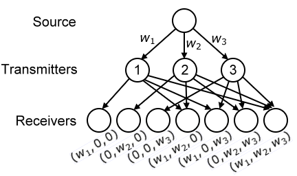
In this section, we will discuss the case where there are d𝑑d transmitters which cooperate to send the same sequence of data {Mi}subscript𝑀𝑖\left\{M_{i}\right\}, but they may or may not be transmitting the same sequence of encoding symbols. There are multiple receivers that wish to decode {Mi}subscript𝑀𝑖\left\{M_{i}\right\} sequentially at different rates. A receiver has an erasure channel connected to each of the d𝑑d transmitters, and the channels may have different capacities. The central question of this section is that, given a set of receivers with different capacities and different rate requirements, is it possible to design a code which can satisfy the need of all receivers?

We call the transmitters as Transmitter kπ‘˜k, where k=1,…,dπ‘˜1…𝑑k=1,...,d. We denote the symbol sent by Transmitter kπ‘˜k at time n𝑛n by Xk,n∈{0,1}subscriptπ‘‹π‘˜π‘›01X_{k,n}\in\{0,1\}. For a receiver with a channel from Transmitter kπ‘˜k with capacity c𝑐c, denote the symbol received from Transmitter kπ‘˜k by Yk,c,n∈{0,1,e}subscriptπ‘Œπ‘˜π‘π‘›01𝑒Y_{k,c,n}\in\{0,1,e\}, and the indicator of erasure Ek,c,n∈{0,1}subscriptπΈπ‘˜π‘π‘›01E_{k,c,n}\in\{0,1\} (Ek,c,n=1subscriptπΈπ‘˜π‘π‘›1E_{k,c,n}=1 indicates an erasure). The definition of a multi-transmitter multi-rate sequential code is similar to that in the single transmitter case, and will be omitted.

For a vector of channel capacities 𝐜∈[0,1]d𝐜superscript01𝑑\mathbf{c}\in[0,1]^{d}, where cksubscriptπ‘π‘˜c_{k} is the capacity of the channel to Transmitter kπ‘˜k, we write

Xnsubscript𝑋𝑛\displaystyle X_{n} =\displaystyle= (X1,n,…,Xd,n),subscript𝑋1𝑛…subscript𝑋𝑑𝑛\displaystyle\left(X_{1,n},...,X_{d,n}\right),
Y𝐜,nsubscriptπ‘Œπœπ‘›\displaystyle Y_{\mathbf{c},n} =\displaystyle= (Y1,c1,n,…,Yd,cd,n),subscriptπ‘Œ1subscript𝑐1𝑛…subscriptπ‘Œπ‘‘subscript𝑐𝑑𝑛\displaystyle\left(Y_{1,c_{1},n},...,Y_{d,c_{d},n}\right),
E𝐜,nsubscriptπΈπœπ‘›\displaystyle E_{\mathbf{c},n} =\displaystyle= (E1,c1,n,…,Ed,cd,n).subscript𝐸1subscript𝑐1𝑛…subscript𝐸𝑑subscript𝑐𝑑𝑛\displaystyle\left(E_{1,c_{1},n},...,E_{d,c_{d},n}\right).

We use the notation Y𝐜,ab=(Y𝐜,a,Y𝐜,a+1,…,Y𝐜,b)superscriptsubscriptπ‘Œπœπ‘Žπ‘subscriptπ‘Œπœπ‘Žsubscriptπ‘Œπœπ‘Ž1…subscriptπ‘Œπœπ‘Y_{\mathbf{c},a}^{b}=(Y_{\mathbf{c},a},Y_{\mathbf{c},a+1},...,Y_{\mathbf{c},b}). From now on, we refer to the receiver with channel capacities 𝐜𝐜\mathbf{c} as Receiver 𝐜𝐜\mathbf{c}. We write the sum of capacities in 𝐜𝐜\mathbf{c} by Σ​(𝐜)=βˆ‘i=1dciΣ𝐜superscriptsubscript𝑖1𝑑subscript𝑐𝑖\Sigma(\mathbf{c})=\sum_{i=1}^{d}c_{i}.

Definition 8 (admissible pair).

A rate-capacity pair (r,𝐜)π‘Ÿπœ(r,\mathbf{c}) is called Ο΅italic-Ο΅\epsilon-admissible by a code if Receiver 𝐜𝐜\mathbf{c} can decode the first N​(rβˆ’Ο΅)π‘π‘Ÿitalic-Ο΅N(r-\epsilon) bits M1N​(rβˆ’Ο΅)superscriptsubscript𝑀1π‘π‘Ÿitalic-Ο΅M_{1}^{N(r-\epsilon)} with bit error probability less than Ο΅italic-Ο΅\epsilon when the first N𝑁N symbols Y𝐜,1Nsuperscriptsubscriptπ‘Œπœ1𝑁Y_{\mathbf{c},1}^{N} are received, for sufficiently large N𝑁N. More precisely, there exist N0subscript𝑁0N_{0} such that

ℙ​{Mmβ‰ M~m​(Q,Y𝐜,1N)}≀ϡ​ for any ​Nβ‰₯N0,m≀N​(rβˆ’Ο΅).formulae-sequenceβ„™subscriptπ‘€π‘šsubscript~π‘€π‘šπ‘„superscriptsubscriptπ‘Œπœ1𝑁italic-ϡ for any 𝑁subscript𝑁0π‘šπ‘π‘Ÿitalic-Ο΅\mathbb{P}\left\{M_{m}\neq\widetilde{M}_{m}\left(Q,Y_{\mathbf{c},1}^{N}\right)\right\}\leq\epsilon\>\text{ for any }N\geq N_{0},m\leq N(r-\epsilon).

We use a function to characterize the rate of a code. We call r:[0,1]dβ†’[0,∞):π‘Ÿβ†’superscript01𝑑0r:[0,1]^{d}\to[0,\infty) a rate-capacity function if it is monotonically increasing and right continuous along each of the d𝑑d dimensions, and there exist an Ξ·>0πœ‚0\eta>0 such that r​(𝐜)=0π‘Ÿπœ0r(\mathbf{c})=0 for Σ​(𝐜)β‰€Ξ·Ξ£πœπœ‚\Sigma(\mathbf{c})\leq\eta.

Definition 9 (rate of MRS code).

A rate-capacity function r​(𝐜)π‘Ÿπœr(\mathbf{c}) is called Ο΅italic-Ο΅\epsilon-admissible by a code if all of the pairs (𝐜,r​(𝐜))πœπ‘Ÿπœ(\mathbf{c},r(\mathbf{c})) are Ο΅italic-Ο΅\epsilon-admissible by the code.

Definition 10 (achievable rate-capacity functions).

A rate-capacity function r​(𝐜)π‘Ÿπœr(\mathbf{c}) is achievable if for any Ο΅>0italic-Ο΅0\epsilon>0, there exist a code where r​(𝐜)π‘Ÿπœr(\mathbf{c}) is Ο΅βˆ’limit-fromitalic-Ο΅\epsilon-admissible by that code.

The superposition MRS code for multiple transmitters is similar to that for single transmitter.

Definition 11 (superposition MRS code).

A superposition MRS code is characterized by the block size K𝐾K and the parameter g:[0,∞)β†’[0,∞)d:𝑔→0superscript0𝑑g:[0,\infty)\to[0,\infty)^{d} which is bounded, monotonically decreasing and left continuous along each dimension with ∫0∞gk​(Ξ±)​𝑑α=1superscriptsubscript0subscriptπ‘”π‘˜π›Όdifferential-d𝛼1\int_{0}^{\infty}g_{k}(\alpha)d\alpha=1 for k=1,…,dπ‘˜1…𝑑k=1,...,d (write gk​(Ξ±)subscriptπ‘”π‘˜π›Όg_{k}(\alpha) for the kπ‘˜k-th entry of g​(Ξ±)𝑔𝛼g(\alpha)). Transmitter kπ‘˜k generates encoding symbols using the single transmitter superposition MRS code with block size K𝐾K and parameter gk​(Ξ±)subscriptπ‘”π‘˜π›Όg_{k}(\alpha).

We say that a rate-capacity function is achievable by superposition MRS code if it is Ο΅βˆ’limit-fromitalic-Ο΅\epsilon-admissible by a superposition MRS code for arbitrarily small Ο΅italic-Ο΅\epsilon. We give the necessary and sufficient condition on the achievability by superposition MRS code.

Theorem 12.

The rate-capacity function r​(𝐜)π‘Ÿπœr(\mathbf{c}) is achievable by superposition MRS code if and only if there exists a function g:[0,∞)β†’[0,∞)d:𝑔→0superscript0𝑑g:[0,\infty)\to[0,\infty)^{d} which is bounded, monotonically decreasing and left continuous along each of the d𝑑d dimensions satisfying

∫0∞gk​(Ξ±)​𝑑α=1​ for ​k=1,…,d,Β andformulae-sequencesuperscriptsubscript0subscriptπ‘”π‘˜π›Όdifferential-d𝛼1Β forΒ π‘˜1…𝑑 and\int_{0}^{\infty}g_{k}(\alpha)d\alpha=1\text{ for }k=1,...,d,\text{ and}
πœβ‹…g​(r​(𝐜))β‰₯1​ for anyΒ β€‹πœβˆˆ[0,1]d​ with ​r​(𝐜)>0.β‹…πœπ‘”π‘Ÿπœ1Β for any 𝐜superscript01𝑑 withΒ π‘Ÿπœ0\mathbf{c}\cdot g\left(r(\mathbf{c})\right)\geq 1\text{ for any }\mathbf{c}\in[0,1]^{d}\text{ with }r(\mathbf{c})>0.
Proof.

The β€œif” part is similar to the proof of achievability in Theorem 7. Fix any Ο΅>0italic-Ο΅0\epsilon>0. Let Ξ·>0πœ‚0\eta>0 such that r​(𝐜)=0π‘Ÿπœ0r(\mathbf{c})=0 for Σ​(𝐜)β‰€Ξ·Ξ£πœπœ‚\Sigma(\mathbf{c})\leq\eta. Define gβ€²:[0,∞)β†’[0,∞)d:superscript𝑔′→0superscript0𝑑g^{\prime}:[0,\infty)\to[0,\infty)^{d} by

gk′​(Ξ±)=(1+ΞΎk)β‹…gk​(Ξ±+Ο΅/2),subscriptsuperscriptπ‘”β€²π‘˜π›Όβ‹…1subscriptπœ‰π‘˜subscriptπ‘”π‘˜π›Όitalic-Ο΅2g^{\prime}_{k}(\alpha)=(1+\xi_{k})\cdot g_{k}(\alpha+\epsilon/2),

where ΞΎk>0subscriptπœ‰π‘˜0\xi_{k}>0 such that ∫0∞gk′​(Ξ±)​𝑑α=1superscriptsubscript0subscriptsuperscriptπ‘”β€²π‘˜π›Όdifferential-d𝛼1\int_{0}^{\infty}g^{\prime}_{k}(\alpha)d\alpha=1. Define a new rate-capacity function r2​(𝐜)=max⁑(r​(𝐜)βˆ’Ο΅/2,0)subscriptπ‘Ÿ2πœπ‘Ÿπœitalic-Ο΅20r_{2}(\mathbf{c})=\max(r(\mathbf{c})-\epsilon/2,0). We have, for any 𝐜𝐜\mathbf{c} with r2​(𝐜)>0subscriptπ‘Ÿ2𝐜0r_{2}(\mathbf{c})>0,

πœβ‹…g′​(r2​(c))=πœβ‹…(1+ΞΎ)​g′​(r2​(𝐜))β‰₯1+ΞΎ.β‹…πœsuperscript𝑔′subscriptπ‘Ÿ2π‘β‹…πœ1πœ‰superscript𝑔′subscriptπ‘Ÿ2𝐜1πœ‰\mathbf{c}\cdot g^{\prime}\left(r_{2}(c)\right)=\mathbf{c}\cdot(1+\xi)g^{\prime}\left(r_{2}(\mathbf{c})\right)\geq 1+\xi.

Consider the multiple transmitter superposition MRS code with parameter g​(Ξ±)𝑔𝛼g(\alpha). Applying Theorem 6 on each dimension, the rate-capacity function r2​(𝐜)subscriptπ‘Ÿ2𝐜r_{2}(\mathbf{c}) is Ο΅/2italic-Ο΅2\epsilon/2-admissible by the code for sufficiently large block size, which implies that r​(𝐜)π‘Ÿπœr(\mathbf{c}) is Ο΅italic-Ο΅\epsilon-admissible by the code.

For the β€œonly if” part, let Ο΅>0italic-Ο΅0\epsilon>0 and consider a superposition MRS code with block size K𝐾K and parameter g​(Ξ±)𝑔𝛼g(\alpha) in which r​(𝐜)π‘Ÿπœr(\mathbf{c}) is Ο΅italic-Ο΅\epsilon-admissible. Consider the receiver with capacities 𝐜𝐜\mathbf{c} which decode at rate r​(𝐜)βˆ’Ο΅π‘Ÿπœitalic-Ο΅r(\mathbf{c})-\epsilon. Using similar arguments as in 6, fixing any block with sufficiently large index, the expected number of times when a received symbol from Transmitter kπ‘˜k is encoded from the block can be given by ck​Kβ‹…gk​(r​(𝐜)βˆ’Ο΅)β‹…subscriptπ‘π‘˜πΎsubscriptπ‘”π‘˜π‘Ÿπœitalic-Ο΅c_{k}K\cdot g_{k}\left(r(\mathbf{c})-\epsilon\right). As at least K𝐾K received symbols is required to decode the block, we have

πœβ‹…g​(r​(𝐜)βˆ’Ο΅)=βˆ‘kck​gk​(r​(𝐜)βˆ’Ο΅)β‰₯1.β‹…πœπ‘”π‘Ÿπœitalic-Ο΅subscriptπ‘˜subscriptπ‘π‘˜subscriptπ‘”π‘˜π‘Ÿπœitalic-Ο΅1\mathbf{c}\cdot g\left(r(\mathbf{c})-\epsilon\right)=\sum_{k}c_{k}g_{k}\left(r(\mathbf{c})-\epsilon\right)\geq 1.

As g​(Ξ±)𝑔𝛼g(\alpha) is left continuous, the proof can be completed by taking Ο΅β†’0β†’italic-Ο΅0\epsilon\to 0. ∎

5. General Non-optimality of Superposition Codes

We have shown in Section 3 that superposition codes are optimal for single transmitter. However, in the multiple transmitter setting, the superposition MRS codes are not optimal in general. We will provide a counter example.

Example 13.

Consider the two transmitter case. Given the block size K𝐾K and 0<r<2/30π‘Ÿ230<r<2/3, the code is constructed by the following process. For Transmitter kπ‘˜k (k=1,2π‘˜12k=1,2), at time i𝑖i, we generate Xk,isubscriptπ‘‹π‘˜π‘–X_{k,i} by taking a random linear combination of the bits in the blocks M2β‹…βŒˆi/(4​K)βŒ‰βˆ’2+kβ€²subscriptsuperscript𝑀′⋅2𝑖4𝐾2π‘˜M^{\prime}_{2\cdot\left\lceil i/(4K)\right\rceil-2+k}, M4β‹…βŒˆi/(4​K)βŒ‰βˆ’1βˆ’kβ€²subscriptsuperscript𝑀′⋅4𝑖4𝐾1π‘˜M^{\prime}_{4\cdot\left\lceil i/(4K)\right\rceil-1-k}, and M4β‹…βŒˆi/(4​K)βŒ‰+1βˆ’kβ€²subscriptsuperscript𝑀′⋅4𝑖4𝐾1π‘˜M^{\prime}_{4\cdot\left\lceil i/(4K)\right\rceil+1-k}, where Miβ€²=M(iβˆ’1)​K+1i​Ksubscriptsuperscript𝑀′𝑖superscriptsubscript𝑀𝑖1𝐾1𝑖𝐾M^{\prime}_{i}=M_{(i-1)K+1}^{iK}.

Consider Transmitter 1, which generates 4​K4𝐾4K encoding bits from the three blocks M2β‹…βŒˆi/(4​K)βŒ‰βˆ’1β€²subscriptsuperscript𝑀′⋅2𝑖4𝐾1M^{\prime}_{2\cdot\left\lceil i/(4K)\right\rceil-1}, M4β‹…βŒˆi/(4​K)βŒ‰βˆ’2β€²subscriptsuperscript𝑀′⋅4𝑖4𝐾2M^{\prime}_{4\cdot\left\lceil i/(4K)\right\rceil-2}, and M4β‹…βŒˆi/(4​K)βŒ‰β€²subscriptsuperscript𝑀′⋅4𝑖4𝐾M^{\prime}_{4\cdot\left\lceil i/(4K)\right\rceil}, with a total of 3​K3𝐾3K bits. Hence, a receiver which can only receive from Transmitter 1 with channel capacity 3/4343/4 can decode the three blocks. When ⌈i/(4​K)βŒ‰=n𝑖4𝐾𝑛\left\lceil i/(4K)\right\rceil=n, the blocks M2​nβˆ’1β€²subscriptsuperscript𝑀′2𝑛1M^{\prime}_{2n-1}, M4​nβˆ’2β€²subscriptsuperscript𝑀′4𝑛2M^{\prime}_{4n-2}, and M4​nβ€²subscriptsuperscript𝑀′4𝑛M^{\prime}_{4n} can be decoded, which covers all the blocks. The rate-capacity pair (12,(34,0))12340\left(\frac{1}{2},(\frac{3}{4},0)\right) is admissible. Similar for (12,(0,34))12034\left(\frac{1}{2},(0,\frac{3}{4})\right).

Consider a receiver which receives from Transmitter 1 and 2, each with channel capacity 1/2121/2. It receives 2​K2𝐾2K bits encoding the three blocks M2β‹…βŒˆi/(4​K)βŒ‰βˆ’1β€²subscriptsuperscript𝑀′⋅2𝑖4𝐾1M^{\prime}_{2\cdot\left\lceil i/(4K)\right\rceil-1}, M4β‹…βŒˆi/(4​K)βŒ‰βˆ’2β€²subscriptsuperscript𝑀′⋅4𝑖4𝐾2M^{\prime}_{4\cdot\left\lceil i/(4K)\right\rceil-2}, M4β‹…βŒˆi/(4​K)βŒ‰β€²subscriptsuperscript𝑀′⋅4𝑖4𝐾M^{\prime}_{4\cdot\left\lceil i/(4K)\right\rceil}, and also 2​K2𝐾2K bits encoding the three blocks M2β‹…βŒˆi/(4​K)βŒ‰β€²subscriptsuperscript𝑀′⋅2𝑖4𝐾M^{\prime}_{2\cdot\left\lceil i/(4K)\right\rceil}, M4β‹…βŒˆi/(4​K)βŒ‰βˆ’3β€²subscriptsuperscript𝑀′⋅4𝑖4𝐾3M^{\prime}_{4\cdot\left\lceil i/(4K)\right\rceil-3}, M4β‹…βŒˆi/(4​K)βŒ‰βˆ’1β€²subscriptsuperscript𝑀′⋅4𝑖4𝐾1M^{\prime}_{4\cdot\left\lceil i/(4K)\right\rceil-1}. When n=d​e​f⌈i/(4​K)βŒ‰=1superscript𝑑𝑒𝑓𝑛𝑖4𝐾1n\stackrel{{\scriptstyle def}}{{=}}\left\lceil i/(4K)\right\rceil=1, the 4​K4𝐾4K bits encoding the blocks M1β€²subscriptsuperscript𝑀′1M^{\prime}_{1} to M4β€²subscriptsuperscript𝑀′4M^{\prime}_{4} are sufficient to decode the blocks. When nβ‰₯2𝑛2n\geq 2, assume the blocks Mmβ€²subscriptsuperscriptπ‘€β€²π‘šM^{\prime}_{m} for m≀4​nβˆ’4π‘š4𝑛4m\leq 4n-4 are already decoded, then there are 2​K2𝐾2K bits encoding the two blocks M4​nβˆ’2β€²subscriptsuperscript𝑀′4𝑛2M^{\prime}_{4n-2} and M4​nβ€²subscriptsuperscript𝑀′4𝑛M^{\prime}_{4n} (M2​nβˆ’1β€²subscriptsuperscript𝑀′2𝑛1M^{\prime}_{2n-1} is already decoded) which are sufficient to decode the blocks, and 2​K2𝐾2K bits encoding the two blocks M4​nβˆ’3β€²subscriptsuperscript𝑀′4𝑛3M^{\prime}_{4n-3} and M4​nβˆ’1β€²subscriptsuperscript𝑀′4𝑛1M^{\prime}_{4n-1} which are sufficient to decode the blocks.The rate-capacity pair (1,(12,12))11212\left(1,(\frac{1}{2},\frac{1}{2})\right) is admissible.

However, the rate-capacity pairs (12,(34,0))12340\left(\frac{1}{2},(\frac{3}{4},0)\right) and (1,(12,12))11212\left(1,(\frac{1}{2},\frac{1}{2})\right) cannot be simultaneously achieved by superposition MRS code. If it can be achieved by superposition MRS code, by Theorem 12, there is a monotonically decreasing function g:[0,∞)↦[0,∞)2:𝑔maps-to0superscript02g:[0,\infty)\mapsto[0,\infty)^{2} satisfying ∫0∞g1​(Ξ±)​𝑑α=∫0∞g2​(Ξ±)​𝑑α=1superscriptsubscript0subscript𝑔1𝛼differential-d𝛼superscriptsubscript0subscript𝑔2𝛼differential-d𝛼1\int_{0}^{\infty}g_{1}(\alpha)d\alpha=\int_{0}^{\infty}g_{2}(\alpha)d\alpha=1 and 34​g1​(12)β‰₯134subscript𝑔1121\frac{3}{4}g_{1}(\frac{1}{2})\geq 1, 12​g1​(1)+12​g2​(1)β‰₯112subscript𝑔1112subscript𝑔211\frac{1}{2}g_{1}(1)+\frac{1}{2}g_{2}(1)\geq 1. As g1​(1),g2​(1)≀1subscript𝑔11subscript𝑔211g_{1}(1),g_{2}(1)\leq 1, we have g1​(1)=g2​(1)=1subscript𝑔11subscript𝑔211g_{1}(1)=g_{2}(1)=1, and g1​(Ξ±)=g2​(Ξ±)=1subscript𝑔1𝛼subscript𝑔2𝛼1g_{1}(\alpha)=g_{2}(\alpha)=1 when α≀1𝛼1\alpha\leq 1, which contradicts with 34​g1​(12)β‰₯134subscript𝑔1121\frac{3}{4}g_{1}(\frac{1}{2})\geq 1.

In the following sections, we will study some special cases in which superposition codes are optimal.

6. Some Useful Tools

We will present some tools which are used to find the admissible region in certain special cases.

For the sake of simplicity, we write

JNβ€‹Ξ±βˆžβ€‹(Y𝐜,1N)superscriptsubscript𝐽𝑁𝛼superscriptsubscriptπ‘Œπœ1𝑁\displaystyle J_{N\alpha}^{\infty}(Y_{\mathbf{c},1}^{N}) =\displaystyle= H​(Y𝐜,1N|M1⌊Nβ€‹Ξ±βŒ‹,E𝐜,1N,Q),Β and𝐻conditionalsuperscriptsubscriptπ‘Œπœ1𝑁superscriptsubscript𝑀1𝑁𝛼superscriptsubscript𝐸𝐜1𝑁𝑄 and\displaystyle H(Y_{\mathbf{c},1}^{N}|M_{1}^{\left\lfloor N\alpha\right\rfloor},E_{\mathbf{c},1}^{N},Q),\text{ and}
JN​αN​β​(Y𝐜,1N)superscriptsubscript𝐽𝑁𝛼𝑁𝛽superscriptsubscriptπ‘Œπœ1𝑁\displaystyle J_{N\alpha}^{N\beta}(Y_{\mathbf{c},1}^{N}) =\displaystyle= I​(M⌊Nβ€‹Ξ±βŒ‹+1⌊Nβ€‹Ξ²βŒ‹;Y𝐜,1N|M1⌊Nβ€‹Ξ±βŒ‹,E𝐜,1N,Q).𝐼superscriptsubscript𝑀𝑁𝛼1𝑁𝛽conditionalsuperscriptsubscriptπ‘Œπœ1𝑁superscriptsubscript𝑀1𝑁𝛼superscriptsubscript𝐸𝐜1𝑁𝑄\displaystyle I(M_{\left\lfloor N\alpha\right\rfloor+1}^{\left\lfloor N\beta\right\rfloor};Y_{\mathbf{c},1}^{N}|M_{1}^{\left\lfloor N\alpha\right\rfloor},E_{\mathbf{c},1}^{N},Q).

We use the infinity sign β€œβˆž\infty” in JNβ€‹Ξ±βˆžβ€‹(Y𝐜,1N)superscriptsubscript𝐽𝑁𝛼superscriptsubscriptπ‘Œπœ1𝑁J_{N\alpha}^{\infty}(Y_{\mathbf{c},1}^{N}) as the encoding symbols Xisubscript𝑋𝑖X_{i} are encoded from M1∞superscriptsubscript𝑀1M_{1}^{\infty} and Q𝑄Q, and Y𝐜,isubscriptπ‘Œπœπ‘–Y_{\mathbf{c},i} can be determined by Xisubscript𝑋𝑖X_{i} and E𝐜,isubscriptπΈπœπ‘–E_{\mathbf{c},i}. As a result,

H​(Y𝐜,1N|M1∞,E𝐜,1N,Q)=0,𝐻conditionalsuperscriptsubscriptπ‘Œπœ1𝑁superscriptsubscript𝑀1superscriptsubscript𝐸𝐜1𝑁𝑄0H(Y_{\mathbf{c},1}^{N}|M_{1}^{\infty},E_{\mathbf{c},1}^{N},Q)=0,

and therefore

JNβ€‹Ξ±βˆžβ€‹(Y𝐜,1N)superscriptsubscript𝐽𝑁𝛼superscriptsubscriptπ‘Œπœ1𝑁\displaystyle J_{N\alpha}^{\infty}(Y_{\mathbf{c},1}^{N}) =\displaystyle= H​(Y𝐜,1N|M1⌊Nβ€‹Ξ±βŒ‹,E𝐜,1N,Q)𝐻conditionalsuperscriptsubscriptπ‘Œπœ1𝑁superscriptsubscript𝑀1𝑁𝛼superscriptsubscript𝐸𝐜1𝑁𝑄\displaystyle H(Y_{\mathbf{c},1}^{N}|M_{1}^{\left\lfloor N\alpha\right\rfloor},E_{\mathbf{c},1}^{N},Q)
=\displaystyle= I​(M⌊Nβ€‹Ξ±βŒ‹+1∞;Y𝐜,1N|M1⌊Nβ€‹Ξ±βŒ‹,E𝐜,1N,Q).𝐼superscriptsubscript𝑀𝑁𝛼1conditionalsuperscriptsubscriptπ‘Œπœ1𝑁superscriptsubscript𝑀1𝑁𝛼superscriptsubscript𝐸𝐜1𝑁𝑄\displaystyle I(M_{\left\lfloor N\alpha\right\rfloor+1}^{\infty};Y_{\mathbf{c},1}^{N}|M_{1}^{\left\lfloor N\alpha\right\rfloor},E_{\mathbf{c},1}^{N},Q).

(Note that the support of M1∞superscriptsubscript𝑀1M_{1}^{\infty} is uncountable. The above equations only serve as the intuition behind the definition.)

The quantity JN​αN​β​(Y𝐜,1N)superscriptsubscript𝐽𝑁𝛼𝑁𝛽superscriptsubscriptπ‘Œπœ1𝑁J_{N\alpha}^{N\beta}(Y_{\mathbf{c},1}^{N}) roughly corresponds to the amount of information in the first N𝑁N encoding symbols dedicated to encode the interval of data M⌊Nβ€‹Ξ±βŒ‹+1⌊Nβ€‹Ξ²βŒ‹superscriptsubscript𝑀𝑁𝛼1𝑁𝛽M_{\left\lfloor N\alpha\right\rfloor+1}^{\left\lfloor N\beta\right\rfloor}. Furthermore, we define

JΒ―Ξ±βˆžβ€‹(Y𝐜,T)superscriptsubscript¯𝐽𝛼subscriptπ‘Œπœπ‘‡\displaystyle\overline{J}_{\alpha}^{\infty}(Y_{\mathbf{c}},T) =\displaystyle= 1Tβ‹…βˆ«0TJΞ±β€‹βŒŠexβŒ‹βˆžβ€‹(Y𝐜,1⌊exβŒ‹)β‹…eβˆ’x​𝑑x,β‹…1𝑇superscriptsubscript0𝑇⋅superscriptsubscript𝐽𝛼superscript𝑒π‘₯superscriptsubscriptπ‘Œπœ1superscript𝑒π‘₯superscript𝑒π‘₯differential-dπ‘₯\displaystyle\frac{1}{T}\cdot\int_{0}^{T}J_{\alpha\left\lfloor e^{x}\right\rfloor}^{\infty}(Y_{\mathbf{c},1}^{\left\lfloor e^{x}\right\rfloor})\cdot e^{-x}dx,
J¯αβ​(Y𝐜,T)superscriptsubscript¯𝐽𝛼𝛽subscriptπ‘Œπœπ‘‡\displaystyle\overline{J}_{\alpha}^{\beta}(Y_{\mathbf{c}},T) =\displaystyle= 1Tβ‹…βˆ«0TJΞ±β€‹βŒŠexβŒ‹Ξ²β€‹βŒŠexβŒ‹β€‹(Y𝐜,1⌊exβŒ‹)β‹…eβˆ’x​𝑑x.β‹…1𝑇superscriptsubscript0𝑇⋅superscriptsubscript𝐽𝛼superscript𝑒π‘₯𝛽superscript𝑒π‘₯superscriptsubscriptπ‘Œπœ1superscript𝑒π‘₯superscript𝑒π‘₯differential-dπ‘₯\displaystyle\frac{1}{T}\cdot\int_{0}^{T}J_{\alpha\left\lfloor e^{x}\right\rfloor}^{\beta\left\lfloor e^{x}\right\rfloor}(Y_{\mathbf{c},1}^{\left\lfloor e^{x}\right\rfloor})\cdot e^{-x}dx.

By observing H​(Y𝐜,1N|E𝐜,1N)≀N​Σ​(𝐜)𝐻conditionalsuperscriptsubscriptπ‘Œπœ1𝑁superscriptsubscript𝐸𝐜1π‘π‘Ξ£πœH(Y_{\mathbf{c},1}^{N}|E_{\mathbf{c},1}^{N})\leq N\Sigma(\mathbf{c}), we know the limits are finite as

1Tβ‹…βˆ«0TJΞ±β€‹βŒŠexβŒ‹Ξ²β€‹βŒŠexβŒ‹β€‹(Y𝐜,1⌊exβŒ‹)β‹…eβˆ’x​𝑑xβ‹…1𝑇superscriptsubscript0𝑇⋅superscriptsubscript𝐽𝛼superscript𝑒π‘₯𝛽superscript𝑒π‘₯superscriptsubscriptπ‘Œπœ1superscript𝑒π‘₯superscript𝑒π‘₯differential-dπ‘₯\displaystyle\frac{1}{T}\cdot\int_{0}^{T}J_{\alpha\left\lfloor e^{x}\right\rfloor}^{\beta\left\lfloor e^{x}\right\rfloor}(Y_{\mathbf{c},1}^{\left\lfloor e^{x}\right\rfloor})\cdot e^{-x}dx
≀\displaystyle\leq 1Tβ‹…βˆ«0TΣ​(𝐜)β€‹βŒŠexβŒ‹β‹…eβˆ’x​𝑑xβ‹…1𝑇superscriptsubscript0π‘‡β‹…Ξ£πœsuperscript𝑒π‘₯superscript𝑒π‘₯differential-dπ‘₯\displaystyle\frac{1}{T}\cdot\int_{0}^{T}\Sigma(\mathbf{c})\left\lfloor e^{x}\right\rfloor\cdot e^{-x}dx
≀\displaystyle\leq Σ​(𝐜),Σ𝐜\displaystyle\Sigma(\mathbf{c}),

and thus

(6.1) J¯αβ​(Y𝐜,T)≀Σ​(𝐜).superscriptsubscript¯𝐽𝛼𝛽subscriptπ‘Œπœπ‘‡Ξ£πœ\overline{J}_{\alpha}^{\beta}(Y_{\mathbf{c}},T)\leq\Sigma(\mathbf{c}).

Similarly, by considering JΞ±β€‹βŒŠexβŒ‹Ξ²β€‹βŒŠexβŒ‹β€‹(Y𝐜,1⌊exβŒ‹)≀(Ξ²βˆ’Ξ±)β€‹βŒŠexβŒ‹superscriptsubscript𝐽𝛼superscript𝑒π‘₯𝛽superscript𝑒π‘₯superscriptsubscriptπ‘Œπœ1superscript𝑒π‘₯𝛽𝛼superscript𝑒π‘₯J_{\alpha\left\lfloor e^{x}\right\rfloor}^{\beta\left\lfloor e^{x}\right\rfloor}(Y_{\mathbf{c},1}^{\left\lfloor e^{x}\right\rfloor})\leq(\beta-\alpha)\left\lfloor e^{x}\right\rfloor, we can obtain

(6.2) J¯αβ​(Y𝐜,T)β‰€Ξ²βˆ’Ξ±.superscriptsubscript¯𝐽𝛼𝛽subscriptπ‘Œπœπ‘‡π›½π›Ό\overline{J}_{\alpha}^{\beta}(Y_{\mathbf{c}},T)\leq\beta-\alpha.

If (𝐜,r)πœπ‘Ÿ(\mathbf{c},r) is Ο΅italic-Ο΅\epsilon-admissible, then whenever rβ‰₯Ξ²>Ξ±β‰₯0π‘Ÿπ›½π›Ό0r\geq\beta>\alpha\geq 0, M⌊Nβ€‹Ξ±βŒ‹+1⌊N​(Ξ²βˆ’Ο΅)βŒ‹superscriptsubscript𝑀𝑁𝛼1𝑁𝛽italic-Ο΅M_{\left\lfloor N\alpha\right\rfloor+1}^{\left\lfloor N(\beta-\epsilon)\right\rfloor} can be decoded using Y𝐜,1Nsuperscriptsubscriptπ‘Œπœ1𝑁Y_{\mathbf{c},1}^{N} for sufficiently large N𝑁N. By Fano’s inequality (note that the case where Ξ²βˆ’Ο΅β‰€Ξ±π›½italic-ϡ𝛼\beta-\epsilon\leq\alpha is obvious),

lim infTβ†’βˆž1Tβ‹…βˆ«0TJΞ±β€‹βŒŠexβŒ‹Ξ²β€‹βŒŠexβŒ‹β€‹(Y𝐜,1⌊exβŒ‹)β‹…eβˆ’x​𝑑xsubscriptlimit-infimum→𝑇⋅1𝑇superscriptsubscript0𝑇⋅superscriptsubscript𝐽𝛼superscript𝑒π‘₯𝛽superscript𝑒π‘₯superscriptsubscriptπ‘Œπœ1superscript𝑒π‘₯superscript𝑒π‘₯differential-dπ‘₯\displaystyle\liminf_{T\to\infty}\frac{1}{T}\cdot\int_{0}^{T}J_{\alpha\left\lfloor e^{x}\right\rfloor}^{\beta\left\lfloor e^{x}\right\rfloor}(Y_{\mathbf{c},1}^{\left\lfloor e^{x}\right\rfloor})\cdot e^{-x}dx
β‰₯\displaystyle\geq lim infTβ†’βˆž1Tβ‹…βˆ«0T(Ξ²βˆ’Ξ±βˆ’Ο΅)​(1βˆ’H​(Ο΅))β€‹βŒŠexβŒ‹β‹…eβˆ’x​𝑑xsubscriptlimit-infimum→𝑇⋅1𝑇superscriptsubscript0𝑇⋅𝛽𝛼italic-Ο΅1𝐻italic-Ο΅superscript𝑒π‘₯superscript𝑒π‘₯differential-dπ‘₯\displaystyle\liminf_{T\to\infty}\frac{1}{T}\cdot\int_{0}^{T}(\beta-\alpha-\epsilon)(1-H(\epsilon))\left\lfloor e^{x}\right\rfloor\cdot e^{-x}dx
=\displaystyle= (Ξ²βˆ’Ξ±βˆ’Ο΅)​(1βˆ’H​(Ο΅)),𝛽𝛼italic-Ο΅1𝐻italic-Ο΅\displaystyle(\beta-\alpha-\epsilon)(1-H(\epsilon)),

and therefore

(6.3) lim infTβ†’βˆžJ¯αβ​(Y𝐜,T)β‰₯(Ξ²βˆ’Ξ±βˆ’Ο΅)​(1βˆ’H​(Ο΅)).subscriptlimit-infimum→𝑇superscriptsubscript¯𝐽𝛼𝛽subscriptπ‘Œπœπ‘‡π›½π›Όitalic-Ο΅1𝐻italic-Ο΅\liminf_{T\to\infty}\overline{J}_{\alpha}^{\beta}(Y_{\mathbf{c}},T)\geq(\beta-\alpha-\epsilon)(1-H(\epsilon)).

Also it is clear that for Ξ³<Ξ±<β𝛾𝛼𝛽\gamma<\alpha<\beta,

(6.4) J¯γβ​(Y𝐜,T)=J¯γα​(Y𝐜,T)+J¯αβ​(Y𝐜,T)superscriptsubscript¯𝐽𝛾𝛽subscriptπ‘Œπœπ‘‡superscriptsubscript¯𝐽𝛾𝛼subscriptπ‘Œπœπ‘‡superscriptsubscript¯𝐽𝛼𝛽subscriptπ‘Œπœπ‘‡\overline{J}_{\gamma}^{\beta}(Y_{\mathbf{c}},T)=\overline{J}_{\gamma}^{\alpha}(Y_{\mathbf{c}},T)+\overline{J}_{\alpha}^{\beta}(Y_{\mathbf{c}},T)

The following lemma can be readily observed.

Lemma 14.

For 𝐜=𝐜1+𝐜2𝐜subscript𝐜1subscript𝐜2\mathbf{c}=\mathbf{c}_{1}+\mathbf{c}_{2}, 𝐜1,𝐜2β‰₯0subscript𝐜1subscript𝐜20\mathbf{c}_{1},\mathbf{c}_{2}\geq 0, we have

J¯αβ​(Y𝐜1,T)≀J¯αβ​(Y𝐜,T)≀J¯αβ​(Y𝐜1,T)+JΒ―Ξ±βˆžβ€‹(Y𝐜2,T).superscriptsubscript¯𝐽𝛼𝛽subscriptπ‘Œsubscript𝐜1𝑇superscriptsubscript¯𝐽𝛼𝛽subscriptπ‘Œπœπ‘‡superscriptsubscript¯𝐽𝛼𝛽subscriptπ‘Œsubscript𝐜1𝑇superscriptsubscript¯𝐽𝛼subscriptπ‘Œsubscript𝐜2𝑇\overline{J}_{\alpha}^{\beta}(Y_{\mathbf{c}_{1}},T)\leq\overline{J}_{\alpha}^{\beta}(Y_{\mathbf{c}},T)\leq\overline{J}_{\alpha}^{\beta}(Y_{\mathbf{c}_{1}},T)+\overline{J}_{\alpha}^{\infty}(Y_{\mathbf{c}_{2}},T).
Proof.

As the quantities depend only on the marginal distributions of {E𝐜,i,Xi,Mi,Q}subscriptπΈπœπ‘–subscript𝑋𝑖subscript𝑀𝑖𝑄\left\{E_{\mathbf{c},i},X_{i},M_{i},Q\right\}, {E𝐜1,i,Xi,Mi,Q}subscript𝐸subscript𝐜1𝑖subscript𝑋𝑖subscript𝑀𝑖𝑄\left\{E_{\mathbf{c}_{1},i},X_{i},M_{i},Q\right\} and {E𝐜2,i,Xi,Mi,Q}subscript𝐸subscript𝐜2𝑖subscript𝑋𝑖subscript𝑀𝑖𝑄\left\{E_{\mathbf{c}_{2},i},X_{i},M_{i},Q\right\}, but not the joint distribution between E𝐜,isubscriptπΈπœπ‘–E_{\mathbf{c},i} and E𝐜1,isubscript𝐸subscript𝐜1𝑖E_{\mathbf{c}_{1},i} and so on. For the purpose of analysis, we assume the non-erasure positions of Receiver 𝐜1subscript𝐜1\mathbf{c}_{1} do not overlap with those of Receiver 𝐜2subscript𝐜2\mathbf{c}_{2}, and erasure happens in Receiver 𝐜𝐜\mathbf{c} if an only if erasure happens in both Receiver 𝐜1subscript𝐜1\mathbf{c}_{1} and Receiver 𝐜2subscript𝐜2\mathbf{c}_{2}. Then Y𝐜,1Nsuperscriptsubscriptπ‘Œπœ1𝑁Y_{\mathbf{c},1}^{N} has the same information as (Y𝐜1,1N,Y𝐜2,1N)superscriptsubscriptπ‘Œsubscript𝐜11𝑁superscriptsubscriptπ‘Œsubscript𝐜21𝑁\left(Y_{\mathbf{c}_{1},1}^{N},Y_{\mathbf{c}_{2},1}^{N}\right). We can deduce from I​(X;Z)≀I​(X,Y;Z)≀I​(X;Z)+H​(Y)πΌπ‘‹π‘πΌπ‘‹π‘Œπ‘πΌπ‘‹π‘π»π‘ŒI(X;Z)\leq I(X,Y;Z)\leq I(X;Z)+H(Y) that

JN​αN​β​(Y𝐜1,1N)≀JN​αN​β​(Y𝐜,1N)≀JN​αN​β​(Y𝐜1,1N)+JNβ€‹Ξ±βˆžβ€‹(Y𝐜2,1N).superscriptsubscript𝐽𝑁𝛼𝑁𝛽superscriptsubscriptπ‘Œsubscript𝐜11𝑁superscriptsubscript𝐽𝑁𝛼𝑁𝛽superscriptsubscriptπ‘Œπœ1𝑁superscriptsubscript𝐽𝑁𝛼𝑁𝛽superscriptsubscriptπ‘Œsubscript𝐜11𝑁superscriptsubscript𝐽𝑁𝛼superscriptsubscriptπ‘Œsubscript𝐜21𝑁J_{N\alpha}^{N\beta}(Y_{\mathbf{c}_{1},1}^{N})\leq J_{N\alpha}^{N\beta}(Y_{\mathbf{c},1}^{N})\leq J_{N\alpha}^{N\beta}(Y_{\mathbf{c}_{1},1}^{N})+J_{N\alpha}^{\infty}(Y_{\mathbf{c}_{2},1}^{N}).

The result follows. ∎

As the message is transmitted in a sequential manner, the received symbols Y𝐜,1Nsuperscriptsubscriptπ‘Œπœ1𝑁Y_{\mathbf{c},1}^{N} should contain more information about the older messages (the Misubscript𝑀𝑖M_{i} with smaller i𝑖i) than newer messages, and therefore the average information (Ξ²βˆ’Ξ±)βˆ’1β‹…J¯αβ​(Y𝐜,T)β‹…superscript𝛽𝛼1superscriptsubscript¯𝐽𝛼𝛽subscriptπ‘Œπœπ‘‡(\beta-\alpha)^{-1}\cdot\overline{J}_{\alpha}^{\beta}(Y_{\mathbf{c}},T) should increase when α𝛼\alpha decrease. This property is proved in the following lemma.

Lemma 15.

Let 0≀γ≀α<Ξ²0𝛾𝛼𝛽0\leq\gamma\leq\alpha<\beta. We have

lim infTβ†’βˆž(1Ξ²βˆ’Ξ³β‹…J¯γβ​(Y𝐜,T)βˆ’1Ξ²βˆ’Ξ±β‹…J¯αβ​(Y𝐜,T))β‰₯0.subscriptlimit-infimum→𝑇⋅1𝛽𝛾superscriptsubscript¯𝐽𝛾𝛽subscriptπ‘Œπœπ‘‡β‹…1𝛽𝛼superscriptsubscript¯𝐽𝛼𝛽subscriptπ‘Œπœπ‘‡0\liminf_{T\to\infty}\left(\frac{1}{\beta-\gamma}\cdot\overline{J}_{\gamma}^{\beta}(Y_{\mathbf{c}},T)-\frac{1}{\beta-\alpha}\cdot\overline{J}_{\alpha}^{\beta}(Y_{\mathbf{c}},T)\right)\geq 0.
Proof.

Consider

JΞ³β€‹βŒŠexβŒ‹Ξ²β€‹βŒŠexβŒ‹β€‹(Y𝐜,1⌊exβŒ‹)superscriptsubscript𝐽𝛾superscript𝑒π‘₯𝛽superscript𝑒π‘₯superscriptsubscriptπ‘Œπœ1superscript𝑒π‘₯\displaystyle J_{\gamma\left\lfloor e^{x}\right\rfloor}^{\beta\left\lfloor e^{x}\right\rfloor}(Y_{\mathbf{c},1}^{\left\lfloor e^{x}\right\rfloor}) =\displaystyle= JΞ±β€‹βŒŠexβŒ‹Ξ²β€‹βŒŠexβŒ‹β€‹(Y𝐜,1⌊exβŒ‹)+JΞ³β€‹βŒŠexβŒ‹Ξ±β€‹βŒŠexβŒ‹β€‹(Y𝐜,1⌊exβŒ‹)superscriptsubscript𝐽𝛼superscript𝑒π‘₯𝛽superscript𝑒π‘₯superscriptsubscriptπ‘Œπœ1superscript𝑒π‘₯superscriptsubscript𝐽𝛾superscript𝑒π‘₯𝛼superscript𝑒π‘₯superscriptsubscriptπ‘Œπœ1superscript𝑒π‘₯\displaystyle J_{\alpha\left\lfloor e^{x}\right\rfloor}^{\beta\left\lfloor e^{x}\right\rfloor}(Y_{\mathbf{c},1}^{\left\lfloor e^{x}\right\rfloor})+J_{\gamma\left\lfloor e^{x}\right\rfloor}^{\alpha\left\lfloor e^{x}\right\rfloor}(Y_{\mathbf{c},1}^{\left\lfloor e^{x}\right\rfloor})
β‰₯\displaystyle\geq JΞ±β€‹βŒŠexβŒ‹Ξ²β€‹βŒŠexβŒ‹β€‹(Y𝐜,1⌊exβŒ‹)+Jγ​exα​ex​(Y𝐜,1⌊exβŒ‹)βˆ’Ξ±.superscriptsubscript𝐽𝛼superscript𝑒π‘₯𝛽superscript𝑒π‘₯superscriptsubscriptπ‘Œπœ1superscript𝑒π‘₯superscriptsubscript𝐽𝛾superscript𝑒π‘₯𝛼superscript𝑒π‘₯superscriptsubscriptπ‘Œπœ1superscript𝑒π‘₯𝛼\displaystyle J_{\alpha\left\lfloor e^{x}\right\rfloor}^{\beta\left\lfloor e^{x}\right\rfloor}(Y_{\mathbf{c},1}^{\left\lfloor e^{x}\right\rfloor})+J_{\gamma e^{x}}^{\alpha e^{x}}(Y_{\mathbf{c},1}^{\left\lfloor e^{x}\right\rfloor})-\alpha.

After integrating the second term, we get, for any x0subscriptπ‘₯0x_{0},

∫x0x0+log⁑(Ξ²/Ξ±)Jγ​exα​ex​(Y𝐜,1⌊exβŒ‹)​𝑑xsuperscriptsubscriptsubscriptπ‘₯0subscriptπ‘₯0𝛽𝛼superscriptsubscript𝐽𝛾superscript𝑒π‘₯𝛼superscript𝑒π‘₯superscriptsubscriptπ‘Œπœ1superscript𝑒π‘₯differential-dπ‘₯\displaystyle\int_{x_{0}}^{x_{0}+\log(\beta/\alpha)}J_{\gamma e^{x}}^{\alpha e^{x}}(Y_{\mathbf{c},1}^{\left\lfloor e^{x}\right\rfloor})dx
β‰₯\displaystyle\geq ∫x0x0+log⁑(Ξ²/Ξ±)Jγ​exα​ex​(Y𝐜,1⌊ex0βŒ‹)​𝑑xsuperscriptsubscriptsubscriptπ‘₯0subscriptπ‘₯0𝛽𝛼superscriptsubscript𝐽𝛾superscript𝑒π‘₯𝛼superscript𝑒π‘₯superscriptsubscriptπ‘Œπœ1superscript𝑒subscriptπ‘₯0differential-dπ‘₯\displaystyle\int_{x_{0}}^{x_{0}+\log(\beta/\alpha)}J_{\gamma e^{x}}^{\alpha e^{x}}(Y_{\mathbf{c},1}^{\left\lfloor e^{x_{0}}\right\rfloor})dx
=\displaystyle= ∫x0x0+log⁑(Ξ²/Ξ±)Jγ​exβˆžβ€‹(Y𝐜,1⌊ex0βŒ‹)​𝑑xβˆ’βˆ«x0x0+log⁑(Ξ²/Ξ±)Jα​exβˆžβ€‹(Y𝐜,1⌊ex0βŒ‹)​𝑑xsuperscriptsubscriptsubscriptπ‘₯0subscriptπ‘₯0𝛽𝛼superscriptsubscript𝐽𝛾superscript𝑒π‘₯superscriptsubscriptπ‘Œπœ1superscript𝑒subscriptπ‘₯0differential-dπ‘₯superscriptsubscriptsubscriptπ‘₯0subscriptπ‘₯0𝛽𝛼superscriptsubscript𝐽𝛼superscript𝑒π‘₯superscriptsubscriptπ‘Œπœ1superscript𝑒subscriptπ‘₯0differential-dπ‘₯\displaystyle\int_{x_{0}}^{x_{0}+\log(\beta/\alpha)}J_{\gamma e^{x}}^{\infty}(Y_{\mathbf{c},1}^{\left\lfloor e^{x_{0}}\right\rfloor})dx-\int_{x_{0}}^{x_{0}+\log(\beta/\alpha)}J_{\alpha e^{x}}^{\infty}(Y_{\mathbf{c},1}^{\left\lfloor e^{x_{0}}\right\rfloor})dx
=\displaystyle= ∫x0βˆ’log⁑(Ξ±/Ξ³)x0βˆ’log⁑(Ξ±/Ξ³)+log⁑(Ξ²/Ξ±)Jγ​ex+log⁑(Ξ±/Ξ³)βˆžβ€‹(Y𝐜,1⌊ex0βŒ‹)​𝑑xβˆ’βˆ«x0x0+log⁑(Ξ²/Ξ±)Jα​exβˆžβ€‹(Y𝐜,1⌊ex0βŒ‹)​𝑑xsuperscriptsubscriptsubscriptπ‘₯0𝛼𝛾subscriptπ‘₯0𝛼𝛾𝛽𝛼superscriptsubscript𝐽𝛾superscript𝑒π‘₯𝛼𝛾superscriptsubscriptπ‘Œπœ1superscript𝑒subscriptπ‘₯0differential-dπ‘₯superscriptsubscriptsubscriptπ‘₯0subscriptπ‘₯0𝛽𝛼superscriptsubscript𝐽𝛼superscript𝑒π‘₯superscriptsubscriptπ‘Œπœ1superscript𝑒subscriptπ‘₯0differential-dπ‘₯\displaystyle\int_{x_{0}-\log(\alpha/\gamma)}^{x_{0}-\log(\alpha/\gamma)+\log(\beta/\alpha)}J_{\gamma e^{x+\log(\alpha/\gamma)}}^{\infty}(Y_{\mathbf{c},1}^{\left\lfloor e^{x_{0}}\right\rfloor})dx-\int_{x_{0}}^{x_{0}+\log(\beta/\alpha)}J_{\alpha e^{x}}^{\infty}(Y_{\mathbf{c},1}^{\left\lfloor e^{x_{0}}\right\rfloor})dx
=\displaystyle= ∫x0βˆ’log⁑(Ξ±/Ξ³)x0+log⁑(β​γ/Ξ±2)Jα​exβˆžβ€‹(Y𝐜,1⌊ex0βŒ‹)​𝑑xβˆ’βˆ«x0x0+log⁑(Ξ²/Ξ±)Jα​exβˆžβ€‹(Y𝐜,1⌊ex0βŒ‹)​𝑑xsuperscriptsubscriptsubscriptπ‘₯0𝛼𝛾subscriptπ‘₯0𝛽𝛾superscript𝛼2superscriptsubscript𝐽𝛼superscript𝑒π‘₯superscriptsubscriptπ‘Œπœ1superscript𝑒subscriptπ‘₯0differential-dπ‘₯superscriptsubscriptsubscriptπ‘₯0subscriptπ‘₯0𝛽𝛼superscriptsubscript𝐽𝛼superscript𝑒π‘₯superscriptsubscriptπ‘Œπœ1superscript𝑒subscriptπ‘₯0differential-dπ‘₯\displaystyle\int_{x_{0}-\log(\alpha/\gamma)}^{x_{0}+\log(\beta\gamma/\alpha^{2})}J_{\alpha e^{x}}^{\infty}(Y_{\mathbf{c},1}^{\left\lfloor e^{x_{0}}\right\rfloor})dx-\int_{x_{0}}^{x_{0}+\log(\beta/\alpha)}J_{\alpha e^{x}}^{\infty}(Y_{\mathbf{c},1}^{\left\lfloor e^{x_{0}}\right\rfloor})dx
=\displaystyle= ∫x0βˆ’log⁑(Ξ±/Ξ³)x0Jα​exβˆžβ€‹(Y𝐜,1⌊ex0βŒ‹)​𝑑xβˆ’βˆ«x0+log⁑(β​γ/Ξ±2)x0+log⁑(Ξ²/Ξ±)Jα​exβˆžβ€‹(Y𝐜,1⌊ex0βŒ‹)​𝑑xsuperscriptsubscriptsubscriptπ‘₯0𝛼𝛾subscriptπ‘₯0superscriptsubscript𝐽𝛼superscript𝑒π‘₯superscriptsubscriptπ‘Œπœ1superscript𝑒subscriptπ‘₯0differential-dπ‘₯superscriptsubscriptsubscriptπ‘₯0𝛽𝛾superscript𝛼2subscriptπ‘₯0𝛽𝛼superscriptsubscript𝐽𝛼superscript𝑒π‘₯superscriptsubscriptπ‘Œπœ1superscript𝑒subscriptπ‘₯0differential-dπ‘₯\displaystyle\int_{x_{0}-\log(\alpha/\gamma)}^{x_{0}}J_{\alpha e^{x}}^{\infty}(Y_{\mathbf{c},1}^{\left\lfloor e^{x_{0}}\right\rfloor})dx-\int_{x_{0}+\log(\beta\gamma/\alpha^{2})}^{x_{0}+\log(\beta/\alpha)}J_{\alpha e^{x}}^{\infty}(Y_{\mathbf{c},1}^{\left\lfloor e^{x_{0}}\right\rfloor})dx
=\displaystyle= ∫x0βˆ’log⁑(Ξ±/Ξ³)x0Jα​exβˆžβ€‹(Y𝐜,1⌊ex0βŒ‹)​𝑑xβˆ’βˆ«x0βˆ’log⁑(Ξ±/Ξ³)x0Jβ​exβˆžβ€‹(Y𝐜,1⌊ex0βŒ‹)​𝑑xsuperscriptsubscriptsubscriptπ‘₯0𝛼𝛾subscriptπ‘₯0superscriptsubscript𝐽𝛼superscript𝑒π‘₯superscriptsubscriptπ‘Œπœ1superscript𝑒subscriptπ‘₯0differential-dπ‘₯superscriptsubscriptsubscriptπ‘₯0𝛼𝛾subscriptπ‘₯0superscriptsubscript𝐽𝛽superscript𝑒π‘₯superscriptsubscriptπ‘Œπœ1superscript𝑒subscriptπ‘₯0differential-dπ‘₯\displaystyle\int_{x_{0}-\log(\alpha/\gamma)}^{x_{0}}J_{\alpha e^{x}}^{\infty}(Y_{\mathbf{c},1}^{\left\lfloor e^{x_{0}}\right\rfloor})dx-\int_{x_{0}-\log(\alpha/\gamma)}^{x_{0}}J_{\beta e^{x}}^{\infty}(Y_{\mathbf{c},1}^{\left\lfloor e^{x_{0}}\right\rfloor})dx
=\displaystyle= ∫x0βˆ’log⁑(Ξ±/Ξ³)x0Jα​exβ​ex​(Y𝐜,1⌊ex0βŒ‹)​𝑑xsuperscriptsubscriptsubscriptπ‘₯0𝛼𝛾subscriptπ‘₯0superscriptsubscript𝐽𝛼superscript𝑒π‘₯𝛽superscript𝑒π‘₯superscriptsubscriptπ‘Œπœ1superscript𝑒subscriptπ‘₯0differential-dπ‘₯\displaystyle\int_{x_{0}-\log(\alpha/\gamma)}^{x_{0}}J_{\alpha e^{x}}^{\beta e^{x}}(Y_{\mathbf{c},1}^{\left\lfloor e^{x_{0}}\right\rfloor})dx
β‰₯\displaystyle\geq ∫x0βˆ’log⁑(Ξ±/Ξ³)x0Jα​exβ​ex​(Y𝐜,1⌊exβŒ‹)​𝑑xsuperscriptsubscriptsubscriptπ‘₯0𝛼𝛾subscriptπ‘₯0superscriptsubscript𝐽𝛼superscript𝑒π‘₯𝛽superscript𝑒π‘₯superscriptsubscriptπ‘Œπœ1superscript𝑒π‘₯differential-dπ‘₯\displaystyle\int_{x_{0}-\log(\alpha/\gamma)}^{x_{0}}J_{\alpha e^{x}}^{\beta e^{x}}(Y_{\mathbf{c},1}^{\left\lfloor e^{x}\right\rfloor})dx
β‰₯\displaystyle\geq ∫x0βˆ’log⁑(Ξ±/Ξ³)x0JΞ±β€‹βŒŠexβŒ‹Ξ²β€‹βŒŠexβŒ‹β€‹(Y𝐜,1⌊exβŒ‹)​𝑑xβˆ’Ξ±β€‹log⁑αγ.superscriptsubscriptsubscriptπ‘₯0𝛼𝛾subscriptπ‘₯0superscriptsubscript𝐽𝛼superscript𝑒π‘₯𝛽superscript𝑒π‘₯superscriptsubscriptπ‘Œπœ1superscript𝑒π‘₯differential-dπ‘₯𝛼𝛼𝛾\displaystyle\int_{x_{0}-\log(\alpha/\gamma)}^{x_{0}}J_{\alpha\left\lfloor e^{x}\right\rfloor}^{\beta\left\lfloor e^{x}\right\rfloor}(Y_{\mathbf{c},1}^{\left\lfloor e^{x}\right\rfloor})dx-\alpha\log\frac{\alpha}{\gamma}.

As a result,

(6.5) ∫x0βˆ’log⁑(Ξ²/Ξ±)x0JΞ³β€‹βŒŠexβŒ‹Ξ²β€‹βŒŠexβŒ‹β€‹(Y𝐜,1⌊exβŒ‹)​𝑑xsuperscriptsubscriptsubscriptπ‘₯0𝛽𝛼subscriptπ‘₯0superscriptsubscript𝐽𝛾superscript𝑒π‘₯𝛽superscript𝑒π‘₯superscriptsubscriptπ‘Œπœ1superscript𝑒π‘₯differential-dπ‘₯\displaystyle\int_{x_{0}-\log(\beta/\alpha)}^{x_{0}}J_{\gamma\left\lfloor e^{x}\right\rfloor}^{\beta\left\lfloor e^{x}\right\rfloor}(Y_{\mathbf{c},1}^{\left\lfloor e^{x}\right\rfloor})dx
β‰₯\displaystyle\geq ∫x0βˆ’log⁑(Ξ²/Ξ±)x0JΞ±β€‹βŒŠexβŒ‹Ξ²β€‹βŒŠexβŒ‹β€‹(Y𝐜,1⌊exβŒ‹)+∫x0βˆ’log⁑(Ξ²/Ξ±)x0Jγ​exα​ex​(Y𝐜,1⌊exβŒ‹)βˆ’Ξ±β€‹log⁑βαsuperscriptsubscriptsubscriptπ‘₯0𝛽𝛼subscriptπ‘₯0superscriptsubscript𝐽𝛼superscript𝑒π‘₯𝛽superscript𝑒π‘₯superscriptsubscriptπ‘Œπœ1superscript𝑒π‘₯superscriptsubscriptsubscriptπ‘₯0𝛽𝛼subscriptπ‘₯0superscriptsubscript𝐽𝛾superscript𝑒π‘₯𝛼superscript𝑒π‘₯superscriptsubscriptπ‘Œπœ1superscript𝑒π‘₯𝛼𝛽𝛼\displaystyle\int_{x_{0}-\log(\beta/\alpha)}^{x_{0}}J_{\alpha\left\lfloor e^{x}\right\rfloor}^{\beta\left\lfloor e^{x}\right\rfloor}(Y_{\mathbf{c},1}^{\left\lfloor e^{x}\right\rfloor})+\int_{x_{0}-\log(\beta/\alpha)}^{x_{0}}J_{\gamma e^{x}}^{\alpha e^{x}}(Y_{\mathbf{c},1}^{\left\lfloor e^{x}\right\rfloor})-\alpha\log\frac{\beta}{\alpha}
β‰₯\displaystyle\geq ∫x0βˆ’log⁑(Ξ²/Ξ±)x0JΞ±β€‹βŒŠexβŒ‹Ξ²β€‹βŒŠexβŒ‹β€‹(Y𝐜,1⌊exβŒ‹)+∫x0βˆ’log⁑(Ξ²/Ξ³)x0βˆ’log⁑(Ξ²/Ξ±)JΞ±β€‹βŒŠexβŒ‹Ξ²β€‹βŒŠexβŒ‹β€‹(Y𝐜,1⌊exβŒ‹)​𝑑xβˆ’Ξ±β€‹log⁑βγsuperscriptsubscriptsubscriptπ‘₯0𝛽𝛼subscriptπ‘₯0superscriptsubscript𝐽𝛼superscript𝑒π‘₯𝛽superscript𝑒π‘₯superscriptsubscriptπ‘Œπœ1superscript𝑒π‘₯superscriptsubscriptsubscriptπ‘₯0𝛽𝛾subscriptπ‘₯0𝛽𝛼superscriptsubscript𝐽𝛼superscript𝑒π‘₯𝛽superscript𝑒π‘₯superscriptsubscriptπ‘Œπœ1superscript𝑒π‘₯differential-dπ‘₯𝛼𝛽𝛾\displaystyle\int_{x_{0}-\log(\beta/\alpha)}^{x_{0}}J_{\alpha\left\lfloor e^{x}\right\rfloor}^{\beta\left\lfloor e^{x}\right\rfloor}(Y_{\mathbf{c},1}^{\left\lfloor e^{x}\right\rfloor})+\int_{x_{0}-\log(\beta/\gamma)}^{x_{0}-\log(\beta/\alpha)}J_{\alpha\left\lfloor e^{x}\right\rfloor}^{\beta\left\lfloor e^{x}\right\rfloor}(Y_{\mathbf{c},1}^{\left\lfloor e^{x}\right\rfloor})dx-\alpha\log\frac{\beta}{\gamma}
β‰₯\displaystyle\geq ∫x0βˆ’log⁑(Ξ²/Ξ³)x0JΞ±β€‹βŒŠexβŒ‹Ξ²β€‹βŒŠexβŒ‹β€‹(Y𝐜,1⌊exβŒ‹)βˆ’Ξ±β€‹log⁑βγ.superscriptsubscriptsubscriptπ‘₯0𝛽𝛾subscriptπ‘₯0superscriptsubscript𝐽𝛼superscript𝑒π‘₯𝛽superscript𝑒π‘₯superscriptsubscriptπ‘Œπœ1superscript𝑒π‘₯𝛼𝛽𝛾\displaystyle\int_{x_{0}-\log(\beta/\gamma)}^{x_{0}}J_{\alpha\left\lfloor e^{x}\right\rfloor}^{\beta\left\lfloor e^{x}\right\rfloor}(Y_{\mathbf{c},1}^{\left\lfloor e^{x}\right\rfloor})-\alpha\log\frac{\beta}{\gamma}.

Fix any T>0𝑇0T>0. For each term in (6.5), multiply it with eβˆ’x0superscript𝑒subscriptπ‘₯0e^{-x_{0}} and integrate it from 0 to T𝑇T, we get

∫0Teβˆ’x0β€‹βˆ«x0βˆ’log⁑(Ξ²/Ξ±)x0JΞ³β€‹βŒŠexβŒ‹Ξ²β€‹βŒŠexβŒ‹β€‹(Y𝐜,1⌊exβŒ‹)​𝑑x​𝑑x0superscriptsubscript0𝑇superscript𝑒subscriptπ‘₯0superscriptsubscriptsubscriptπ‘₯0𝛽𝛼subscriptπ‘₯0superscriptsubscript𝐽𝛾superscript𝑒π‘₯𝛽superscript𝑒π‘₯superscriptsubscriptπ‘Œπœ1superscript𝑒π‘₯differential-dπ‘₯differential-dsubscriptπ‘₯0\displaystyle\int_{0}^{T}e^{-x_{0}}\int_{x_{0}-\log(\beta/\alpha)}^{x_{0}}J_{\gamma\left\lfloor e^{x}\right\rfloor}^{\beta\left\lfloor e^{x}\right\rfloor}(Y_{\mathbf{c},1}^{\left\lfloor e^{x}\right\rfloor})dxdx_{0}
=\displaystyle= ∫0T∫xmin⁑(T,x+log⁑(Ξ²/Ξ±))eβˆ’x0​JΞ³β€‹βŒŠexβŒ‹Ξ²β€‹βŒŠexβŒ‹β€‹(Y𝐜,1⌊exβŒ‹)​𝑑x0​𝑑xsuperscriptsubscript0𝑇superscriptsubscriptπ‘₯𝑇π‘₯𝛽𝛼superscript𝑒subscriptπ‘₯0superscriptsubscript𝐽𝛾superscript𝑒π‘₯𝛽superscript𝑒π‘₯superscriptsubscriptπ‘Œπœ1superscript𝑒π‘₯differential-dsubscriptπ‘₯0differential-dπ‘₯\displaystyle\int_{0}^{T}\int_{x}^{\min\left(T,x+\log(\beta/\alpha)\right)}e^{-x_{0}}J_{\gamma\left\lfloor e^{x}\right\rfloor}^{\beta\left\lfloor e^{x}\right\rfloor}(Y_{\mathbf{c},1}^{\left\lfloor e^{x}\right\rfloor})dx_{0}dx
≀\displaystyle\leq ∫0T∫xx+log⁑(Ξ²/Ξ±)eβˆ’x0​JΞ³β€‹βŒŠexβŒ‹Ξ²β€‹βŒŠexβŒ‹β€‹(Y𝐜,1⌊exβŒ‹)​𝑑x0​𝑑xsuperscriptsubscript0𝑇superscriptsubscriptπ‘₯π‘₯𝛽𝛼superscript𝑒subscriptπ‘₯0superscriptsubscript𝐽𝛾superscript𝑒π‘₯𝛽superscript𝑒π‘₯superscriptsubscriptπ‘Œπœ1superscript𝑒π‘₯differential-dsubscriptπ‘₯0differential-dπ‘₯\displaystyle\int_{0}^{T}\int_{x}^{x+\log(\beta/\alpha)}e^{-x_{0}}J_{\gamma\left\lfloor e^{x}\right\rfloor}^{\beta\left\lfloor e^{x}\right\rfloor}(Y_{\mathbf{c},1}^{\left\lfloor e^{x}\right\rfloor})dx_{0}dx
=\displaystyle= (1βˆ’Ξ±Ξ²)β€‹βˆ«0Teβˆ’x​JΞ³β€‹βŒŠexβŒ‹Ξ²β€‹βŒŠexβŒ‹β€‹(Y𝐜,1⌊exβŒ‹)​𝑑x.1𝛼𝛽superscriptsubscript0𝑇superscript𝑒π‘₯superscriptsubscript𝐽𝛾superscript𝑒π‘₯𝛽superscript𝑒π‘₯superscriptsubscriptπ‘Œπœ1superscript𝑒π‘₯differential-dπ‘₯\displaystyle\left(1-\frac{\alpha}{\beta}\right)\int_{0}^{T}e^{-x}J_{\gamma\left\lfloor e^{x}\right\rfloor}^{\beta\left\lfloor e^{x}\right\rfloor}(Y_{\mathbf{c},1}^{\left\lfloor e^{x}\right\rfloor})dx.

And also

∫0Teβˆ’x0β€‹βˆ«x0βˆ’log⁑(Ξ²/Ξ³)x0JΞ±β€‹βŒŠexβŒ‹Ξ²β€‹βŒŠexβŒ‹β€‹(Y𝐜,1⌊exβŒ‹)​𝑑x​𝑑x0superscriptsubscript0𝑇superscript𝑒subscriptπ‘₯0superscriptsubscriptsubscriptπ‘₯0𝛽𝛾subscriptπ‘₯0superscriptsubscript𝐽𝛼superscript𝑒π‘₯𝛽superscript𝑒π‘₯superscriptsubscriptπ‘Œπœ1superscript𝑒π‘₯differential-dπ‘₯differential-dsubscriptπ‘₯0\displaystyle\int_{0}^{T}e^{-x_{0}}\int_{x_{0}-\log(\beta/\gamma)}^{x_{0}}J_{\alpha\left\lfloor e^{x}\right\rfloor}^{\beta\left\lfloor e^{x}\right\rfloor}(Y_{\mathbf{c},1}^{\left\lfloor e^{x}\right\rfloor})dxdx_{0}
=\displaystyle= ∫0T∫xmin⁑(T,x+log⁑(Ξ²/Ξ³))eβˆ’x0​JΞ±β€‹βŒŠexβŒ‹Ξ²β€‹βŒŠexβŒ‹β€‹(Y𝐜,1⌊exβŒ‹)​𝑑x0​𝑑xsuperscriptsubscript0𝑇superscriptsubscriptπ‘₯𝑇π‘₯𝛽𝛾superscript𝑒subscriptπ‘₯0superscriptsubscript𝐽𝛼superscript𝑒π‘₯𝛽superscript𝑒π‘₯superscriptsubscriptπ‘Œπœ1superscript𝑒π‘₯differential-dsubscriptπ‘₯0differential-dπ‘₯\displaystyle\int_{0}^{T}\int_{x}^{\min\left(T,x+\log(\beta/\gamma)\right)}e^{-x_{0}}J_{\alpha\left\lfloor e^{x}\right\rfloor}^{\beta\left\lfloor e^{x}\right\rfloor}(Y_{\mathbf{c},1}^{\left\lfloor e^{x}\right\rfloor})dx_{0}dx
β‰₯\displaystyle\geq ∫0Tβˆ’log⁑(Ξ²/Ξ³)∫xx+log⁑(Ξ²/Ξ³)eβˆ’x0​JΞ±β€‹βŒŠexβŒ‹Ξ²β€‹βŒŠexβŒ‹β€‹(Y𝐜,1⌊exβŒ‹)​𝑑x0​𝑑xsuperscriptsubscript0𝑇𝛽𝛾superscriptsubscriptπ‘₯π‘₯𝛽𝛾superscript𝑒subscriptπ‘₯0superscriptsubscript𝐽𝛼superscript𝑒π‘₯𝛽superscript𝑒π‘₯superscriptsubscriptπ‘Œπœ1superscript𝑒π‘₯differential-dsubscriptπ‘₯0differential-dπ‘₯\displaystyle\int_{0}^{T-\log(\beta/\gamma)}\int_{x}^{x+\log(\beta/\gamma)}e^{-x_{0}}J_{\alpha\left\lfloor e^{x}\right\rfloor}^{\beta\left\lfloor e^{x}\right\rfloor}(Y_{\mathbf{c},1}^{\left\lfloor e^{x}\right\rfloor})dx_{0}dx
=\displaystyle= (1βˆ’Ξ³Ξ²)β€‹βˆ«0Tβˆ’log⁑(Ξ²/Ξ³)eβˆ’x​JΞ±β€‹βŒŠexβŒ‹Ξ²β€‹βŒŠexβŒ‹β€‹(Y𝐜,1⌊exβŒ‹)​𝑑x1𝛾𝛽superscriptsubscript0𝑇𝛽𝛾superscript𝑒π‘₯superscriptsubscript𝐽𝛼superscript𝑒π‘₯𝛽superscript𝑒π‘₯superscriptsubscriptπ‘Œπœ1superscript𝑒π‘₯differential-dπ‘₯\displaystyle\left(1-\frac{\gamma}{\beta}\right)\int_{0}^{T-\log(\beta/\gamma)}e^{-x}J_{\alpha\left\lfloor e^{x}\right\rfloor}^{\beta\left\lfloor e^{x}\right\rfloor}(Y_{\mathbf{c},1}^{\left\lfloor e^{x}\right\rfloor})dx
β‰₯\displaystyle\geq (1βˆ’Ξ³Ξ²)β€‹βˆ«0Teβˆ’x​JΞ±β€‹βŒŠexβŒ‹Ξ²β€‹βŒŠexβŒ‹β€‹(Y𝐜,1⌊exβŒ‹)​𝑑xβˆ’(1βˆ’Ξ³Ξ²)​(Ξ²βˆ’Ξ±)​log⁑βγ.1𝛾𝛽superscriptsubscript0𝑇superscript𝑒π‘₯superscriptsubscript𝐽𝛼superscript𝑒π‘₯𝛽superscript𝑒π‘₯superscriptsubscriptπ‘Œπœ1superscript𝑒π‘₯differential-dπ‘₯1𝛾𝛽𝛽𝛼𝛽𝛾\displaystyle\left(1-\frac{\gamma}{\beta}\right)\int_{0}^{T}e^{-x}J_{\alpha\left\lfloor e^{x}\right\rfloor}^{\beta\left\lfloor e^{x}\right\rfloor}(Y_{\mathbf{c},1}^{\left\lfloor e^{x}\right\rfloor})dx-\left(1-\frac{\gamma}{\beta}\right)(\beta-\alpha)\log\frac{\beta}{\gamma}.

Therefore, by (6.5),

(1βˆ’Ξ±Ξ²)β€‹βˆ«0Teβˆ’x​JΞ³β€‹βŒŠexβŒ‹Ξ²β€‹βŒŠexβŒ‹β€‹(Y𝐜,1⌊exβŒ‹)​𝑑x1𝛼𝛽superscriptsubscript0𝑇superscript𝑒π‘₯superscriptsubscript𝐽𝛾superscript𝑒π‘₯𝛽superscript𝑒π‘₯superscriptsubscriptπ‘Œπœ1superscript𝑒π‘₯differential-dπ‘₯\displaystyle\left(1-\frac{\alpha}{\beta}\right)\int_{0}^{T}e^{-x}J_{\gamma\left\lfloor e^{x}\right\rfloor}^{\beta\left\lfloor e^{x}\right\rfloor}(Y_{\mathbf{c},1}^{\left\lfloor e^{x}\right\rfloor})dx
β‰₯\displaystyle\geq (1βˆ’Ξ³Ξ²)β€‹βˆ«0Teβˆ’x​JΞ±β€‹βŒŠexβŒ‹Ξ²β€‹βŒŠexβŒ‹β€‹(Y𝐜,1⌊exβŒ‹)​𝑑xβˆ’(1βˆ’Ξ³Ξ²)​(Ξ²βˆ’Ξ±)​logβ‘Ξ²Ξ³βˆ’βˆ«0Teβˆ’x0​α​log⁑βγ​d​x01𝛾𝛽superscriptsubscript0𝑇superscript𝑒π‘₯superscriptsubscript𝐽𝛼superscript𝑒π‘₯𝛽superscript𝑒π‘₯superscriptsubscriptπ‘Œπœ1superscript𝑒π‘₯differential-dπ‘₯1𝛾𝛽𝛽𝛼𝛽𝛾superscriptsubscript0𝑇superscript𝑒subscriptπ‘₯0𝛼𝛽𝛾𝑑subscriptπ‘₯0\displaystyle\left(1-\frac{\gamma}{\beta}\right)\int_{0}^{T}e^{-x}J_{\alpha\left\lfloor e^{x}\right\rfloor}^{\beta\left\lfloor e^{x}\right\rfloor}(Y_{\mathbf{c},1}^{\left\lfloor e^{x}\right\rfloor})dx-\left(1-\frac{\gamma}{\beta}\right)(\beta-\alpha)\log\frac{\beta}{\gamma}-\int_{0}^{T}e^{-x_{0}}\alpha\log\frac{\beta}{\gamma}dx_{0}
=\displaystyle= (1βˆ’Ξ³Ξ²)β€‹βˆ«0Teβˆ’x​JΞ±β€‹βŒŠexβŒ‹Ξ²β€‹βŒŠexβŒ‹β€‹(Y𝐜,1⌊exβŒ‹)​𝑑xβˆ’(1βˆ’Ξ³Ξ²)​(Ξ²βˆ’Ξ±)​logβ‘Ξ²Ξ³βˆ’(1βˆ’eβˆ’T)​α​log⁑βγ1𝛾𝛽superscriptsubscript0𝑇superscript𝑒π‘₯superscriptsubscript𝐽𝛼superscript𝑒π‘₯𝛽superscript𝑒π‘₯superscriptsubscriptπ‘Œπœ1superscript𝑒π‘₯differential-dπ‘₯1𝛾𝛽𝛽𝛼𝛽𝛾1superscript𝑒𝑇𝛼𝛽𝛾\displaystyle\left(1-\frac{\gamma}{\beta}\right)\int_{0}^{T}e^{-x}J_{\alpha\left\lfloor e^{x}\right\rfloor}^{\beta\left\lfloor e^{x}\right\rfloor}(Y_{\mathbf{c},1}^{\left\lfloor e^{x}\right\rfloor})dx-\left(1-\frac{\gamma}{\beta}\right)(\beta-\alpha)\log\frac{\beta}{\gamma}-\left(1-e^{-T}\right)\alpha\log\frac{\beta}{\gamma}
β‰₯\displaystyle\geq (1βˆ’Ξ³Ξ²)β€‹βˆ«0Teβˆ’x​JΞ±β€‹βŒŠexβŒ‹Ξ²β€‹βŒŠexβŒ‹β€‹(Y𝐜,1⌊exβŒ‹)​𝑑xβˆ’((Ξ²βˆ’Ξ±)​(Ξ²βˆ’Ξ³)Ξ²+Ξ±)β‹…log⁑βγ1𝛾𝛽superscriptsubscript0𝑇superscript𝑒π‘₯superscriptsubscript𝐽𝛼superscript𝑒π‘₯𝛽superscript𝑒π‘₯superscriptsubscriptπ‘Œπœ1superscript𝑒π‘₯differential-dπ‘₯⋅𝛽𝛼𝛽𝛾𝛽𝛼𝛽𝛾\displaystyle\left(1-\frac{\gamma}{\beta}\right)\int_{0}^{T}e^{-x}J_{\alpha\left\lfloor e^{x}\right\rfloor}^{\beta\left\lfloor e^{x}\right\rfloor}(Y_{\mathbf{c},1}^{\left\lfloor e^{x}\right\rfloor})dx-\left(\frac{(\beta-\alpha)(\beta-\gamma)}{\beta}+\alpha\right)\cdot\log\frac{\beta}{\gamma}

Multiply Ξ²/(Tβ‹…(Ξ²βˆ’Ξ±)​(Ξ²βˆ’Ξ³))𝛽⋅𝑇𝛽𝛼𝛽𝛾\beta/\left(T\cdot(\beta-\alpha)(\beta-\gamma)\right) to both sides, we can obtain

1Ξ²βˆ’Ξ³β‹…1Tβ‹…βˆ«0Teβˆ’x​JΞ³β€‹βŒŠexβŒ‹Ξ²β€‹βŒŠexβŒ‹β€‹(Y𝐜,1⌊exβŒ‹)​𝑑xβ‹…1𝛽𝛾1𝑇superscriptsubscript0𝑇superscript𝑒π‘₯superscriptsubscript𝐽𝛾superscript𝑒π‘₯𝛽superscript𝑒π‘₯superscriptsubscriptπ‘Œπœ1superscript𝑒π‘₯differential-dπ‘₯\displaystyle\frac{1}{\beta-\gamma}\cdot\frac{1}{T}\cdot\int_{0}^{T}e^{-x}J_{\gamma\left\lfloor e^{x}\right\rfloor}^{\beta\left\lfloor e^{x}\right\rfloor}(Y_{\mathbf{c},1}^{\left\lfloor e^{x}\right\rfloor})dx
β‰₯\displaystyle\geq 1Ξ²βˆ’Ξ±β‹…1Tβ‹…βˆ«0Teβˆ’x​JΞ±β€‹βŒŠexβŒ‹Ξ²β€‹βŒŠexβŒ‹β€‹(Y𝐜,1⌊exβŒ‹)​𝑑xβˆ’1Tβ‹…(1+α​β(Ξ²βˆ’Ξ±)​(Ξ²βˆ’Ξ³))β‹…log⁑βγ.β‹…1𝛽𝛼1𝑇superscriptsubscript0𝑇superscript𝑒π‘₯superscriptsubscript𝐽𝛼superscript𝑒π‘₯𝛽superscript𝑒π‘₯superscriptsubscriptπ‘Œπœ1superscript𝑒π‘₯differential-dπ‘₯β‹…1𝑇1𝛼𝛽𝛽𝛼𝛽𝛾𝛽𝛾\displaystyle\frac{1}{\beta-\alpha}\cdot\frac{1}{T}\cdot\int_{0}^{T}e^{-x}J_{\alpha\left\lfloor e^{x}\right\rfloor}^{\beta\left\lfloor e^{x}\right\rfloor}(Y_{\mathbf{c},1}^{\left\lfloor e^{x}\right\rfloor})dx-\frac{1}{T}\cdot\left(1+\frac{\alpha\beta}{(\beta-\alpha)(\beta-\gamma)}\right)\cdot\log\frac{\beta}{\gamma}.

Note that the second term vanishes when Tβ†’βˆžβ†’π‘‡T\to\infty. The result follows. ∎

We now proceed to prove an inequality on achievable rate-capacity functions.

Lemma 16.

If a rate-capacity function r​(𝐜)π‘Ÿπœr(\mathbf{c}) is achievable, then for any 𝐜=𝐜1+𝐜2+…+𝐜n𝐜subscript𝐜1subscript𝐜2…subscriptπœπ‘›\mathbf{c}=\mathbf{c}_{1}+\mathbf{c}_{2}+...+\mathbf{c}_{n}, where 𝐜kβ‰₯0subscriptπœπ‘˜0\mathbf{c}_{k}\geq 0 and r​(𝐜)>r​(𝐜k)π‘Ÿπœπ‘Ÿsubscriptπœπ‘˜r(\mathbf{c})>r(\mathbf{c}_{k}) for k=1,…,nπ‘˜1…𝑛k=1,...,n, we have

βˆ‘k=1nΣ​(𝐜k)βˆ’r​(𝐜k)r​(𝐜)βˆ’r​(𝐜k)β‰₯1.superscriptsubscriptπ‘˜1𝑛Σsubscriptπœπ‘˜π‘Ÿsubscriptπœπ‘˜π‘Ÿπœπ‘Ÿsubscriptπœπ‘˜1\sum_{k=1}^{n}\frac{\Sigma(\mathbf{c}_{k})-r(\mathbf{c}_{k})}{r(\mathbf{c})-r(\mathbf{c}_{k})}\geq 1.
Proof.

Without loss of generality, assume r​(𝐜1)≀…≀r​(𝐜n)<r​(𝐜)π‘Ÿsubscript𝐜1β€¦π‘Ÿsubscriptπœπ‘›π‘Ÿπœr(\mathbf{c}_{1})\leq...\leq r(\mathbf{c}_{n})<r(\mathbf{c}). Let 𝐜0=0subscript𝐜00\mathbf{c}_{0}=0. Consider a code in which r​(𝐜)π‘Ÿπœr(\mathbf{c}) is Ο΅βˆ’limit-fromitalic-Ο΅\epsilon-admissible. Fix any k∈{1,…,n}π‘˜1…𝑛k\in\{1,...,n\}. By (6.1), for any Tβ‰₯0𝑇0T\geq 0,

JΒ―0βˆžβ€‹(Y𝐜k,T)≀Σ​(𝐜k).superscriptsubscript¯𝐽0subscriptπ‘Œsubscriptπœπ‘˜π‘‡Ξ£subscriptπœπ‘˜\overline{J}_{0}^{\infty}(Y_{\mathbf{c}_{k}},T)\leq\Sigma(\mathbf{c}_{k}).

By (6.4),

JΒ―r​(𝐜k)βˆžβ€‹(Y𝐜k,T)superscriptsubscriptΒ―π½π‘Ÿsubscriptπœπ‘˜subscriptπ‘Œsubscriptπœπ‘˜π‘‡\displaystyle\overline{J}_{r(\mathbf{c}_{k})}^{\infty}(Y_{\mathbf{c}_{k}},T) =\displaystyle= JΒ―0βˆžβ€‹(Y𝐜k,T)βˆ’JΒ―0r​(𝐜k)​(Y𝐜k,T)superscriptsubscript¯𝐽0subscriptπ‘Œsubscriptπœπ‘˜π‘‡superscriptsubscript¯𝐽0π‘Ÿsubscriptπœπ‘˜subscriptπ‘Œsubscriptπœπ‘˜π‘‡\displaystyle\overline{J}_{0}^{\infty}(Y_{\mathbf{c}_{k}},T)-\overline{J}_{0}^{r(\mathbf{c}_{k})}(Y_{\mathbf{c}_{k}},T)
≀\displaystyle\leq Σ​(𝐜k)βˆ’JΒ―0r​(𝐜k)​(Y𝐜k,T).Ξ£subscriptπœπ‘˜superscriptsubscript¯𝐽0π‘Ÿsubscriptπœπ‘˜subscriptπ‘Œsubscriptπœπ‘˜π‘‡\displaystyle\Sigma(\mathbf{c}_{k})-\overline{J}_{0}^{r(\mathbf{c}_{k})}(Y_{\mathbf{c}_{k}},T).

Invoking Lemma 14, we obtain

JΒ―r​(𝐜k)r​(𝐜)​(Y𝐜1+…+𝐜kβˆ’1,T)superscriptsubscriptΒ―π½π‘Ÿsubscriptπœπ‘˜π‘Ÿπœsubscriptπ‘Œsubscript𝐜1…subscriptπœπ‘˜1𝑇\displaystyle\overline{J}_{r(\mathbf{c}_{k})}^{r(\mathbf{c})}(Y_{\mathbf{c}_{1}+...+\mathbf{c}_{k-1}},T) β‰₯\displaystyle\geq JΒ―r​(𝐜k)r​(𝐜)​(Y𝐜1+…+𝐜k,T)βˆ’JΒ―r​(𝐜k)βˆžβ€‹(Y𝐜k,T)superscriptsubscriptΒ―π½π‘Ÿsubscriptπœπ‘˜π‘Ÿπœsubscriptπ‘Œsubscript𝐜1…subscriptπœπ‘˜π‘‡superscriptsubscriptΒ―π½π‘Ÿsubscriptπœπ‘˜subscriptπ‘Œsubscriptπœπ‘˜π‘‡\displaystyle\overline{J}_{r(\mathbf{c}_{k})}^{r(\mathbf{c})}(Y_{\mathbf{c}_{1}+...+\mathbf{c}_{k}},T)-\overline{J}_{r(\mathbf{c}_{k})}^{\infty}(Y_{\mathbf{c}_{k}},T)
β‰₯\displaystyle\geq JΒ―r​(𝐜k)r​(𝐜)​(Y𝐜1+…+𝐜k,T)βˆ’Ξ£β€‹(𝐜k)+JΒ―0r​(𝐜k)​(Y𝐜k,T),superscriptsubscriptΒ―π½π‘Ÿsubscriptπœπ‘˜π‘Ÿπœsubscriptπ‘Œsubscript𝐜1…subscriptπœπ‘˜π‘‡Ξ£subscriptπœπ‘˜superscriptsubscript¯𝐽0π‘Ÿsubscriptπœπ‘˜subscriptπ‘Œsubscriptπœπ‘˜π‘‡\displaystyle\overline{J}_{r(\mathbf{c}_{k})}^{r(\mathbf{c})}(Y_{\mathbf{c}_{1}+...+\mathbf{c}_{k}},T)-\Sigma(\mathbf{c}_{k})+\overline{J}_{0}^{r(\mathbf{c}_{k})}(Y_{\mathbf{c}_{k}},T),

It can be deduced using Lemma 15 that

lim infTβ†’βˆž(1r​(𝐜)βˆ’r​(𝐜kβˆ’1)JΒ―r​(𝐜kβˆ’1)r​(𝐜)(Y𝐜1+…+𝐜kβˆ’1,T)\displaystyle\liminf_{T\to\infty}\Biggl{(}\frac{1}{r(\mathbf{c})-r(\mathbf{c}_{k-1})}\overline{J}_{r(\mathbf{c}_{k-1})}^{r(\mathbf{c})}(Y_{\mathbf{c}_{1}+...+\mathbf{c}_{k-1}},T)
βˆ’1r​(𝐜)βˆ’r​(𝐜k)JΒ―r​(𝐜k)r​(𝐜)(Y𝐜1+…+𝐜kβˆ’1,T))\displaystyle-\frac{1}{r(\mathbf{c})-r(\mathbf{c}_{k})}\overline{J}_{r(\mathbf{c}_{k})}^{r(\mathbf{c})}(Y_{\mathbf{c}_{1}+...+\mathbf{c}_{k-1}},T)\Biggr{)} β‰₯\displaystyle\geq 0,0\displaystyle 0,

and therefore

lim infTβ†’βˆž(1r​(𝐜)βˆ’r​(𝐜kβˆ’1)JΒ―r​(𝐜kβˆ’1)r​(𝐜)(Y𝐜1+…+𝐜kβˆ’1,T)\displaystyle\liminf_{T\to\infty}\Biggl{(}\frac{1}{r(\mathbf{c})-r(\mathbf{c}_{k-1})}\overline{J}_{r(\mathbf{c}_{k-1})}^{r(\mathbf{c})}(Y_{\mathbf{c}_{1}+...+\mathbf{c}_{k-1}},T)
βˆ’1r​(𝐜)βˆ’r​(𝐜k)JΒ―r​(𝐜k)r​(𝐜)(Y𝐜1+…+𝐜k,T)+Σ​(𝐜k)βˆ’JΒ―0r​(𝐜k)​(Y𝐜k,T)r​(𝐜)βˆ’r​(𝐜k))\displaystyle-\frac{1}{r(\mathbf{c})-r(\mathbf{c}_{k})}\overline{J}_{r(\mathbf{c}_{k})}^{r(\mathbf{c})}(Y_{\mathbf{c}_{1}+...+\mathbf{c}_{k}},T)+\frac{\Sigma(\mathbf{c}_{k})-\overline{J}_{0}^{r(\mathbf{c}_{k})}(Y_{\mathbf{c}_{k}},T)}{r(\mathbf{c})-r(\mathbf{c}_{k})}\Biggr{)} β‰₯\displaystyle\geq 0,0\displaystyle 0,

Summing through k=1,…,nπ‘˜1…𝑛k=1,...,n,

lim infTβ†’βˆž(1r​(𝐜)βˆ’r​(0)JΒ―r​(0)r​(𝐜)(Y𝐜0,T)\displaystyle\liminf_{T\to\infty}\Biggl{(}\frac{1}{r(\mathbf{c})-r(0)}\overline{J}_{r(0)}^{r(\mathbf{c})}(Y_{\mathbf{c}_{0}},T)
βˆ’1r​(𝐜)βˆ’r​(𝐜n)JΒ―r​(𝐜n)r​(𝐜)(Y𝐜,T)+βˆ‘k=1nΣ​(𝐜k)βˆ’JΒ―0r​(𝐜k)​(Y𝐜k,T)r​(𝐜)βˆ’r​(𝐜k))\displaystyle-\frac{1}{r(\mathbf{c})-r(\mathbf{c}_{n})}\overline{J}_{r(\mathbf{c}_{n})}^{r(\mathbf{c})}(Y_{\mathbf{c}},T)+\sum_{k=1}^{n}\frac{\Sigma(\mathbf{c}_{k})-\overline{J}_{0}^{r(\mathbf{c}_{k})}(Y_{\mathbf{c}_{k}},T)}{r(\mathbf{c})-r(\mathbf{c}_{k})}\Biggr{)} β‰₯\displaystyle\geq 0,0\displaystyle 0,

and thus

lim infTβ†’βˆž(βˆ‘k=1nΣ​(𝐜k)βˆ’JΒ―0r​(𝐜k)​(Y𝐜k,T)r​(𝐜)βˆ’r​(𝐜k)\displaystyle\liminf_{T\to\infty}\Biggl{(}\sum_{k=1}^{n}\frac{\Sigma(\mathbf{c}_{k})-\overline{J}_{0}^{r(\mathbf{c}_{k})}(Y_{\mathbf{c}_{k}},T)}{r(\mathbf{c})-r(\mathbf{c}_{k})}
βˆ’1r​(𝐜)βˆ’r​(𝐜n)JΒ―r​(𝐜n)r​(𝐜)(Y𝐜,T))\displaystyle-\frac{1}{r(\mathbf{c})-r(\mathbf{c}_{n})}\overline{J}_{r(\mathbf{c}_{n})}^{r(\mathbf{c})}(Y_{\mathbf{c}},T)\Biggr{)} β‰₯\displaystyle\geq 0,0\displaystyle 0,

Using (6.3), we have

lim infTβ†’βˆžJΒ―0r​(𝐜k)​(Y𝐜k,T)β‰₯(r​(𝐜k)βˆ’Ο΅)​(1βˆ’H​(Ο΅)),subscriptlimit-infimum→𝑇superscriptsubscript¯𝐽0π‘Ÿsubscriptπœπ‘˜subscriptπ‘Œsubscriptπœπ‘˜π‘‡π‘Ÿsubscriptπœπ‘˜italic-Ο΅1𝐻italic-Ο΅\liminf_{T\to\infty}\overline{J}_{0}^{r(\mathbf{c}_{k})}(Y_{\mathbf{c}_{k}},T)\geq\left(r(\mathbf{c}_{k})-\epsilon\right)\left(1-H(\epsilon)\right),

and

lim infTβ†’βˆžJΒ―r​(𝐜n)r​(𝐜)​(Y𝐜,T)β‰₯(r​(𝐜)βˆ’r​(𝐜n)βˆ’Ο΅)​(1βˆ’H​(Ο΅)).subscriptlimit-infimum→𝑇superscriptsubscriptΒ―π½π‘Ÿsubscriptπœπ‘›π‘Ÿπœsubscriptπ‘Œπœπ‘‡π‘Ÿπœπ‘Ÿsubscriptπœπ‘›italic-Ο΅1𝐻italic-Ο΅\liminf_{T\to\infty}\overline{J}_{r(\mathbf{c}_{n})}^{r(\mathbf{c})}(Y_{\mathbf{c}},T)\geq\left(r(\mathbf{c})-r(\mathbf{c}_{n})-\epsilon\right)\left(1-H(\epsilon)\right).

Hence,

βˆ‘k=1nΣ​(𝐜k)βˆ’(r​(𝐜k)βˆ’Ο΅)​(1βˆ’H​(Ο΅))r​(𝐜)βˆ’r​(𝐜k)superscriptsubscriptπ‘˜1𝑛Σsubscriptπœπ‘˜π‘Ÿsubscriptπœπ‘˜italic-Ο΅1𝐻italic-Ο΅π‘Ÿπœπ‘Ÿsubscriptπœπ‘˜\displaystyle\sum_{k=1}^{n}\frac{\Sigma(\mathbf{c}_{k})-\left(r(\mathbf{c}_{k})-\epsilon\right)\left(1-H(\epsilon)\right)}{r(\mathbf{c})-r(\mathbf{c}_{k})}
βˆ’(r​(𝐜)βˆ’r​(𝐜n)βˆ’Ο΅)​(1βˆ’H​(Ο΅))r​(𝐜)βˆ’r​(𝐜n)π‘Ÿπœπ‘Ÿsubscriptπœπ‘›italic-Ο΅1𝐻italic-Ο΅π‘Ÿπœπ‘Ÿsubscriptπœπ‘›\displaystyle-\frac{\left(r(\mathbf{c})-r(\mathbf{c}_{n})-\epsilon\right)\left(1-H(\epsilon)\right)}{r(\mathbf{c})-r(\mathbf{c}_{n})} β‰₯\displaystyle\geq 0.0\displaystyle 0.

Let Ο΅β†’0β†’italic-Ο΅0\epsilon\to 0. We obtained the desired result as

βˆ‘k=1nΣ​(𝐜k)βˆ’r​(𝐜k)r​(𝐜)βˆ’r​(𝐜k)β‰₯1.superscriptsubscriptπ‘˜1𝑛Σsubscriptπœπ‘˜π‘Ÿsubscriptπœπ‘˜π‘Ÿπœπ‘Ÿsubscriptπœπ‘˜1\sum_{k=1}^{n}\frac{\Sigma(\mathbf{c}_{k})-r(\mathbf{c}_{k})}{r(\mathbf{c})-r(\mathbf{c}_{k})}\geq 1.

∎

We will discuss some cases in which superposition coding is provably optimal in the next section.

7. On-Off Multicast Networks

In this section, we consider networks in which there are d𝑑d transmitters and 2dβˆ’1superscript2𝑑12^{d}-1 receivers, each having a different set of transmitters to which it is connected. Transmitter kπ‘˜k broadcasts the same information to the receivers it is connected to at rate wksubscriptπ‘€π‘˜w_{k}. Each receiver has to decode the information at a different rate. There is no erasure in the network. We would like to formulate the criteria on the decoding rates of the receivers in which sequential data transmission is possible.

We first convert the problem into the multi-transmitter MRS setting. Without loss of generality, we assume wk≀1subscriptπ‘€π‘˜1w_{k}\leq 1 for k=1,…,dπ‘˜1…𝑑k=1,...,d. We may replace a connection with rate w𝑀w by an erasure channel with capacity w𝑀w. Note that the decoding requirement does not depend on the joint distribution of erasure events of different receivers. Therefore, the problem can be translated to d𝑑d-transmitter MRS. We confine our study to the capacity vectors 𝐜∈{0,w1}×…×{0,wd}𝐜0subscript𝑀1…0subscript𝑀𝑑\mathbf{c}\in\{0,w_{1}\}\times...\times\{0,w_{d}\}.

Refer to caption
Figure 7.1. A three-transmitter on-off multicast network

7.1. Non-optimality of superposition coding in general

We can construct a network in which superposition coding is not optimal, using a similar idea as in Example 13.

Example 17.

The network contains 3 transmitters and 3 receivers, where Transmitter 1 and 2 broadcast at rate 1, and Transmitter 3 broadcast at rate 2. Receiver 1 is connected to Transmitter 1 and 2. Receiver 2 is connected to Transmitter 1 and 3. Receiver 3 is connected to Transmitter 2 and 3. Non-superposition code can achieve the decoding rate 3/2323/2 for Receiver 1, and 333 for Receiver 2 and 3, which are not achievable using superposition codes. Please refer to Subsection 7.3 for the proof of achievability and further discussions.
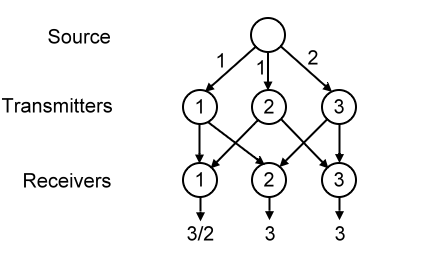
Refer to caption
Figure 7.2. The network in which superposition codes are not optimal

Although superposition coding is not optimal for networks with 3 transmitters in general, it is optimal for networks with 2 transmitters, which will be shown in the following example.

7.2. One-or-all on-off multicast network

Example 18 (One-or-all on-off multicast network).

There are d𝑑d transmitters and d+1𝑑1d+1 receivers (numbered 0,…,d𝑑d), where Transmitter kπ‘˜k broadcasts the same information to Receiver 0 and kπ‘˜k at rate of wksubscriptπ‘€π‘˜w_{k} bit/s for k=1,…,dπ‘˜1…𝑑k=1,...,d. Receiver kπ‘˜k has to decode the data at rate rksubscriptπ‘Ÿπ‘˜r_{k} bit/s for k=0,…,dπ‘˜0…𝑑k=0,...,d. We would like to characterize the achievable region of {rk}subscriptπ‘Ÿπ‘˜\left\{r_{k}\right\} in terms of {wk}subscriptπ‘€π‘˜\left\{w_{k}\right\}. Figure 7.3 shows the network when d=2𝑑2d=2.

Refer to caption
Figure 7.3. The two-transmitter one-or-all on-off multicast network

The following theorem shows that superposition coding is optimal.

Theorem 19.

Superposition coding is optimal in the one-or-all on-off multicast network, which has an achievable region

r0β‰₯0, 0≀rk≀wk​ for ​k=1,…,d,formulae-sequenceformulae-sequencesubscriptπ‘Ÿ00 0subscriptπ‘Ÿπ‘˜subscriptπ‘€π‘˜Β forΒ π‘˜1…𝑑r_{0}\geq 0,\,0\leq r_{k}\leq w_{k}\text{ for }k=1,...,d,
either ​r0≀max⁑(wk)​ orΒ β€‹βˆ‘k=1dwkβˆ’rkr0βˆ’rkβ‰₯1.eitherΒ subscriptπ‘Ÿ0subscriptπ‘€π‘˜Β orΒ superscriptsubscriptπ‘˜1𝑑subscriptπ‘€π‘˜subscriptπ‘Ÿπ‘˜subscriptπ‘Ÿ0subscriptπ‘Ÿπ‘˜1\text{either }r_{0}\leq\max(w_{k})\text{ or }\sum_{k=1}^{d}\frac{w_{k}-r_{k}}{r_{0}-r_{k}}\geq 1.
Proof.

The case where r0≀max⁑(wk)subscriptπ‘Ÿ0subscriptπ‘€π‘˜r_{0}\leq\max(w_{k}) is trivial. We assume r0>wksubscriptπ‘Ÿ0subscriptπ‘€π‘˜r_{0}>w_{k} for all kπ‘˜k. Without loss of generality, assume r1≀…≀rdsubscriptπ‘Ÿ1…subscriptπ‘Ÿπ‘‘r_{1}\leq...\leq r_{d}, then we have r1≀…≀rd≀wd<r0subscriptπ‘Ÿ1…subscriptπ‘Ÿπ‘‘subscript𝑀𝑑subscriptπ‘Ÿ0r_{1}\leq...\leq r_{d}\leq w_{d}<r_{0}.

Among the inequalities in the proposed achievable region, rk≀wksubscriptπ‘Ÿπ‘˜subscriptπ‘€π‘˜r_{k}\leq w_{k} is obvious, and βˆ‘k=1dwkβˆ’rkr0βˆ’rkβ‰₯1superscriptsubscriptπ‘˜1𝑑subscriptπ‘€π‘˜subscriptπ‘Ÿπ‘˜subscriptπ‘Ÿ0subscriptπ‘Ÿπ‘˜1\sum_{k=1}^{d}\frac{w_{k}-r_{k}}{r_{0}-r_{k}}\geq 1 is due to Lemma 16. The converse follows.

We now show superposition MRS code can achieve the region. Assume βˆ‘k=1dwkβˆ’rkr0βˆ’rkβ‰₯1superscriptsubscriptπ‘˜1𝑑subscriptπ‘€π‘˜subscriptπ‘Ÿπ‘˜subscriptπ‘Ÿ0subscriptπ‘Ÿπ‘˜1\sum_{k=1}^{d}\frac{w_{k}-r_{k}}{r_{0}-r_{k}}\geq 1. Consider the parameter

gk​(Ξ±)={1wkΒ when ​α≀rkwkβˆ’rkwk​(r0βˆ’rk)Β when ​rk<α≀r00Β when ​α>r0.subscriptπ‘”π‘˜π›Όcases1subscriptπ‘€π‘˜Β when 𝛼subscriptπ‘Ÿπ‘˜subscriptπ‘€π‘˜subscriptπ‘Ÿπ‘˜subscriptπ‘€π‘˜subscriptπ‘Ÿ0subscriptπ‘Ÿπ‘˜Β whenΒ subscriptπ‘Ÿπ‘˜π›Όsubscriptπ‘Ÿ00Β when 𝛼subscriptπ‘Ÿ0g_{k}(\alpha)=\begin{cases}\frac{1}{w_{k}}&\text{ when }\alpha\leq r_{k}\\ \frac{w_{k}-r_{k}}{w_{k}(r_{0}-r_{k})}&\text{ when }r_{k}<\alpha\leq r_{0}\\ 0&\text{ when }\alpha>r_{0}.\end{cases}

Note that

wkβˆ’rkwk​(r0βˆ’rk)≀1wksubscriptπ‘€π‘˜subscriptπ‘Ÿπ‘˜subscriptπ‘€π‘˜subscriptπ‘Ÿ0subscriptπ‘Ÿπ‘˜1subscriptπ‘€π‘˜\frac{w_{k}-r_{k}}{w_{k}(r_{0}-r_{k})}\leq\frac{1}{w_{k}}

due to r0β‰₯wksubscriptπ‘Ÿ0subscriptπ‘€π‘˜r_{0}\geq w_{k}. Therefore g​(Ξ±)𝑔𝛼g(\alpha) is monotonically decreasing along each dimension. It can be easily checked that ∫0∞gk​(Ξ±)​𝑑α=1superscriptsubscript0subscriptπ‘”π‘˜π›Όdifferential-d𝛼1\int_{0}^{\infty}g_{k}(\alpha)d\alpha=1. It is left to check πœβ‹…g​(r​(𝐜))β‰₯1β‹…πœπ‘”π‘Ÿπœ1\mathbf{c}\cdot g(r(\mathbf{c}))\geq 1.

wkβ‹…gk​(rk)=wkβ‹…1wk=1,β‹…subscriptπ‘€π‘˜subscriptπ‘”π‘˜subscriptπ‘Ÿπ‘˜β‹…subscriptπ‘€π‘˜1subscriptπ‘€π‘˜1w_{k}\cdot g_{k}(r_{k})=w_{k}\cdot\frac{1}{w_{k}}=1,
βˆ‘k=1dwkβ‹…gk​(r0)superscriptsubscriptπ‘˜1𝑑⋅subscriptπ‘€π‘˜subscriptπ‘”π‘˜subscriptπ‘Ÿ0\displaystyle\sum_{k=1}^{d}w_{k}\cdot g_{k}(r_{0})
=\displaystyle= βˆ‘k=1dwkβ‹…wkβˆ’rkwk​(r0βˆ’rk)superscriptsubscriptπ‘˜1𝑑⋅subscriptπ‘€π‘˜subscriptπ‘€π‘˜subscriptπ‘Ÿπ‘˜subscriptπ‘€π‘˜subscriptπ‘Ÿ0subscriptπ‘Ÿπ‘˜\displaystyle\sum_{k=1}^{d}w_{k}\cdot\frac{w_{k}-r_{k}}{w_{k}(r_{0}-r_{k})}
=\displaystyle= βˆ‘k=1dwkβˆ’rkr0βˆ’rkβ‰₯1.superscriptsubscriptπ‘˜1𝑑subscriptπ‘€π‘˜subscriptπ‘Ÿπ‘˜subscriptπ‘Ÿ0subscriptπ‘Ÿπ‘˜1\displaystyle\sum_{k=1}^{d}\frac{w_{k}-r_{k}}{r_{0}-r_{k}}\geq 1.

By Theorem 12, the region is achievable by superposition MRS code.∎

Remark.

The achievable region in the MRS setting is different from that in multilevel diversity coding, which admits the larger region

r0β‰₯0, 0≀rk≀wk​ for ​k=1,…,d,r0+βˆ‘k=1drkβˆ’maxk=1,…,d⁑(rk)β‰€βˆ‘k=1dwk.formulae-sequenceformulae-sequencesubscriptπ‘Ÿ00 0subscriptπ‘Ÿπ‘˜subscriptπ‘€π‘˜Β forΒ π‘˜1…𝑑subscriptπ‘Ÿ0superscriptsubscriptπ‘˜1𝑑subscriptπ‘Ÿπ‘˜subscriptπ‘˜1…𝑑subscriptπ‘Ÿπ‘˜superscriptsubscriptπ‘˜1𝑑subscriptπ‘€π‘˜r_{0}\geq 0,\,0\leq r_{k}\leq w_{k}\text{ for }k=1,...,d,\,r_{0}+\sum_{k=1}^{d}r_{k}-\max_{k=1,...,d}(r_{k})\leq\sum_{k=1}^{d}w_{k}.

7.3. Non-superposition codes

In Example 17, we presented a network in which superposition codes are non-optimal. Even though non-superposition codes are used, the tools described in Section 6 may still be used. We are going to prove the achievable region of a generalized version of Example 17.

Example 20.

There are 333 transmitters and 333 receivers numbered 1,2,333. Receiver 1 receives from Transmitter 1 and 2, and wish to decode at r1subscriptπ‘Ÿ1r_{1}. Receiver 2 receives from Transmitter 1 and 3, and wish to decode at r2β‰₯r1subscriptπ‘Ÿ2subscriptπ‘Ÿ1r_{2}\geq r_{1}. Receiver 3 receives from Transmitter 2 and 3, and wish to decode at r3=r2subscriptπ‘Ÿ3subscriptπ‘Ÿ2r_{3}=r_{2}.

Refer to caption
Figure 7.4. The network specified in Example 20

The achievable region is given by the following theorem.

Theorem 21.

The achievable region in Example 20 can be given by

w1+w2subscript𝑀1subscript𝑀2\displaystyle w_{1}+w_{2} β‰₯\displaystyle\geq r1subscriptπ‘Ÿ1\displaystyle r_{1}
w1+w3subscript𝑀1subscript𝑀3\displaystyle w_{1}+w_{3} β‰₯\displaystyle\geq r2subscriptπ‘Ÿ2\displaystyle r_{2}
w2+w3subscript𝑀2subscript𝑀3\displaystyle w_{2}+w_{3} β‰₯\displaystyle\geq r2subscriptπ‘Ÿ2\displaystyle r_{2}
w1+w2+w3β‹…r2βˆ’r1r2subscript𝑀1subscript𝑀2β‹…subscript𝑀3subscriptπ‘Ÿ2subscriptπ‘Ÿ1subscriptπ‘Ÿ2\displaystyle w_{1}+w_{2}+w_{3}\cdot\frac{r_{2}-r_{1}}{r_{2}} β‰₯\displaystyle\geq r2.subscriptπ‘Ÿ2\displaystyle r_{2}.
Proof of converse.

The first three inequalities clearly hold. For the last inequality, consider a code in which the rate requirements are Ο΅βˆ’limit-fromitalic-Ο΅\epsilon-admissible. Receiver 1 can decode at rate r1subscriptπ‘Ÿ1r_{1}. By (6.3),

JΒ―0r1​(Y(w1,w2,0))β‰₯(r1βˆ’Ο΅)​(1βˆ’H​(Ο΅)).superscriptsubscript¯𝐽0subscriptπ‘Ÿ1subscriptπ‘Œsubscript𝑀1subscript𝑀20subscriptπ‘Ÿ1italic-Ο΅1𝐻italic-Ο΅\underline{J}_{0}^{r_{1}}(Y_{(w_{1},w_{2},0)})\geq\left(r_{1}-\epsilon\right)\left(1-H(\epsilon)\right).

Invoking (6.1) and Lemma 14, we can obtain

(7.1) JΒ―0r1​(Y(w1,0,0))+w2superscriptsubscript¯𝐽0subscriptπ‘Ÿ1subscriptπ‘Œsubscript𝑀100subscript𝑀2\displaystyle\underline{J}_{0}^{r_{1}}(Y_{(w_{1},0,0)})+w_{2} β‰₯\displaystyle\geq JΒ―0r1​(Y(w1,0,0))+JΒ―0βˆžβ€‹(Y(0,w2,0))superscriptsubscript¯𝐽0subscriptπ‘Ÿ1subscriptπ‘Œsubscript𝑀100superscriptsubscript¯𝐽0subscriptπ‘Œ0subscript𝑀20\displaystyle\underline{J}_{0}^{r_{1}}(Y_{(w_{1},0,0)})+\overline{J}_{0}^{\infty}(Y_{(0,w_{2},0)})
β‰₯\displaystyle\geq JΒ―0r1​(Y(w1,w2,0))superscriptsubscript¯𝐽0subscriptπ‘Ÿ1subscriptπ‘Œsubscript𝑀1subscript𝑀20\displaystyle\underline{J}_{0}^{r_{1}}(Y_{(w_{1},w_{2},0)})
β‰₯\displaystyle\geq (r1βˆ’Ο΅)​(1βˆ’H​(Ο΅)).subscriptπ‘Ÿ1italic-Ο΅1𝐻italic-Ο΅\displaystyle\left(r_{1}-\epsilon\right)\left(1-H(\epsilon)\right).

Receiver 2 can decode at rate r2subscriptπ‘Ÿ2r_{2}. By (6.3),

JΒ―r1r2​(Y(w1,0,w3))β‰₯(r2βˆ’r1βˆ’Ο΅)​(1βˆ’H​(Ο΅)).superscriptsubscript¯𝐽subscriptπ‘Ÿ1subscriptπ‘Ÿ2subscriptπ‘Œsubscript𝑀10subscript𝑀3subscriptπ‘Ÿ2subscriptπ‘Ÿ1italic-Ο΅1𝐻italic-Ο΅\underline{J}_{r_{1}}^{r_{2}}(Y_{(w_{1},0,w_{3})})\geq\left(r_{2}-r_{1}-\epsilon\right)\left(1-H(\epsilon)\right).

Invoking Lemma 14, we can obtain

JΒ―r1βˆžβ€‹(Y(w1,0,0))+JΒ―r1r2​(Y(0,0,w3))superscriptsubscript¯𝐽subscriptπ‘Ÿ1subscriptπ‘Œsubscript𝑀100superscriptsubscript¯𝐽subscriptπ‘Ÿ1subscriptπ‘Ÿ2subscriptπ‘Œ00subscript𝑀3\displaystyle\overline{J}_{r_{1}}^{\infty}(Y_{(w_{1},0,0)})+\underline{J}_{r_{1}}^{r_{2}}(Y_{(0,0,w_{3})}) β‰₯\displaystyle\geq JΒ―r1r2​(Y(w1,0,w3))superscriptsubscript¯𝐽subscriptπ‘Ÿ1subscriptπ‘Ÿ2subscriptπ‘Œsubscript𝑀10subscript𝑀3\displaystyle\underline{J}_{r_{1}}^{r_{2}}(Y_{(w_{1},0,w_{3})})
β‰₯\displaystyle\geq (r2βˆ’r1βˆ’Ο΅)​(1βˆ’H​(Ο΅)).subscriptπ‘Ÿ2subscriptπ‘Ÿ1italic-Ο΅1𝐻italic-Ο΅\displaystyle\left(r_{2}-r_{1}-\epsilon\right)\left(1-H(\epsilon)\right).

By Lemma 15 and (6.1),

w3β‰₯JΒ―0r2​(Y(0,0,w3))β‰₯r2r2βˆ’r1β‹…JΒ―r1r2​(Y(0,0,w3)),subscript𝑀3superscriptsubscript¯𝐽0subscriptπ‘Ÿ2subscriptπ‘Œ00subscript𝑀3β‹…subscriptπ‘Ÿ2subscriptπ‘Ÿ2subscriptπ‘Ÿ1superscriptsubscript¯𝐽subscriptπ‘Ÿ1subscriptπ‘Ÿ2subscriptπ‘Œ00subscript𝑀3w_{3}\geq\underline{J}_{0}^{r_{2}}(Y_{(0,0,w_{3})})\geq\frac{r_{2}}{r_{2}-r_{1}}\cdot\underline{J}_{r_{1}}^{r_{2}}(Y_{(0,0,w_{3})}),

and therefore

(7.2) JΒ―r1βˆžβ€‹(Y(w1,0,0))+r2βˆ’r1r2β‹…w3β‰₯(r2βˆ’r1βˆ’Ο΅)​(1βˆ’H​(Ο΅)).superscriptsubscript¯𝐽subscriptπ‘Ÿ1subscriptπ‘Œsubscript𝑀100β‹…subscriptπ‘Ÿ2subscriptπ‘Ÿ1subscriptπ‘Ÿ2subscript𝑀3subscriptπ‘Ÿ2subscriptπ‘Ÿ1italic-Ο΅1𝐻italic-Ο΅\overline{J}_{r_{1}}^{\infty}(Y_{(w_{1},0,0)})+\frac{r_{2}-r_{1}}{r_{2}}\cdot w_{3}\geq\left(r_{2}-r_{1}-\epsilon\right)\left(1-H(\epsilon)\right).

By (6.1) and (6.4),

(7.3) w1subscript𝑀1\displaystyle w_{1} β‰₯\displaystyle\geq JΒ―0βˆžβ€‹(Y(w1,0,0))superscriptsubscript¯𝐽0subscriptπ‘Œsubscript𝑀100\displaystyle\overline{J}_{0}^{\infty}(Y_{(w_{1},0,0)})
β‰₯\displaystyle\geq JΒ―0r1​(Y(w1,0,0))+JΒ―r1βˆžβ€‹(Y(w1,0,0)).superscriptsubscript¯𝐽0subscriptπ‘Ÿ1subscriptπ‘Œsubscript𝑀100superscriptsubscript¯𝐽subscriptπ‘Ÿ1subscriptπ‘Œsubscript𝑀100\displaystyle\underline{J}_{0}^{r_{1}}(Y_{(w_{1},0,0)})+\overline{J}_{r_{1}}^{\infty}(Y_{(w_{1},0,0)}).

Adding (7.1), (7.2) and (7.3),

w1+w2+r2βˆ’r1r2β‹…w3β‰₯(r2βˆ’2​ϡ)​(1βˆ’H​(Ο΅)).subscript𝑀1subscript𝑀2β‹…subscriptπ‘Ÿ2subscriptπ‘Ÿ1subscriptπ‘Ÿ2subscript𝑀3subscriptπ‘Ÿ22italic-Ο΅1𝐻italic-Ο΅w_{1}+w_{2}+\frac{r_{2}-r_{1}}{r_{2}}\cdot w_{3}\geq\left(r_{2}-2\epsilon\right)\left(1-H(\epsilon)\right).

The proof can be completed by taking Ο΅β†’0β†’italic-Ο΅0\epsilon\to 0. ∎

 
Proof of achievability.

We will describe a coding scheme which can achieve the proposed region. When r1=r2subscriptπ‘Ÿ1subscriptπ‘Ÿ2r_{1}=r_{2}, we may use all the transmitters to transmit at rate r1subscriptπ‘Ÿ1r_{1}. When w3β‰₯r2subscript𝑀3subscriptπ‘Ÿ2w_{3}\geq r_{2}, then we can use Transmitter 3 alone to transmit the message at rate r2subscriptπ‘Ÿ2r_{2}, and Transmitter 1 together with Transmitter 2 to transmit at rate r1subscriptπ‘Ÿ1r_{1}. Therefore we assume r1<r2subscriptπ‘Ÿ1subscriptπ‘Ÿ2r_{1}<r_{2} and w3<r2subscript𝑀3subscriptπ‘Ÿ2w_{3}<r_{2}.

The code is specified by the block size K𝐾K, the super-block size L>K𝐿𝐾L>K, and the parameter γ𝛾\gamma. Divide the message {Mi}i=1,2,…subscriptsubscript𝑀𝑖𝑖12…\left\{M_{i}\right\}_{i=1,2,...} into blocks of K𝐾K bits Bi=M(iβˆ’1)​K+1i​Ksubscript𝐡𝑖superscriptsubscript𝑀𝑖1𝐾1𝑖𝐾B_{i}=M_{(i-1)K+1}^{iK}. Further divide each block Bisubscript𝐡𝑖B_{i} into two sub-blocks B1,isubscript𝐡1𝑖B_{1,i} and B2,isubscript𝐡2𝑖B_{2,i}, where B1,isubscript𝐡1𝑖B_{1,i} contains the first γ​K𝛾𝐾\gamma K bits of the block, where γ𝛾\gamma is taken to be w3/r2subscript𝑀3subscriptπ‘Ÿ2w_{3}/r_{2} in this case, and B2,isubscript𝐡2𝑖B_{2,i} contains the rest of the bits. Group the sub-blocks into super-blocks by

Sa,b,i=(Bb,(iβˆ’1)β‹…raβ‹…L/K+1,…,Bb,iβ‹…raβ‹…L/K)subscriptπ‘†π‘Žπ‘π‘–subscript𝐡𝑏⋅𝑖1subscriptπ‘Ÿπ‘ŽπΏπΎ1…subscript𝐡𝑏⋅𝑖subscriptπ‘Ÿπ‘ŽπΏπΎS_{a,b,i}=\left(B_{b,(i-1)\cdot r_{a}\cdot L/K+1},...,B_{b,i\cdot r_{a}\cdot L/K}\right)

for a,b∈{1,2}π‘Žπ‘12a,b\in\{1,2\}. Assume r1β‹…L/Kβ‹…subscriptπ‘Ÿ1𝐿𝐾r_{1}\cdot L/K and r2β‹…L/Kβ‹…subscriptπ‘Ÿ2𝐿𝐾r_{2}\cdot L/K are integers. Each super-block Sa,1,isubscriptπ‘†π‘Ž1𝑖S_{a,1,i} contains ra⋅γ​Lβ‹…subscriptπ‘Ÿπ‘Žπ›ΎπΏr_{a}\cdot\gamma L bits, and each super-block Sa,2,isubscriptπ‘†π‘Ž2𝑖S_{a,2,i} contains raβ‹…(1βˆ’Ξ³)​Lβ‹…subscriptπ‘Ÿπ‘Ž1𝛾𝐿r_{a}\cdot(1-\gamma)L bits.

Refer to caption
Figure 7.5. The super-blocks when Ξ³=2/3𝛾23\gamma=2/3 and r2=2​r1subscriptπ‘Ÿ22subscriptπ‘Ÿ1r_{2}=2r_{1}

At time i𝑖i, Transmitter 1 encodes the super-blocks S1,1,⌈i/LβŒ‰subscript𝑆11𝑖𝐿S_{1,1,\left\lceil i/L\right\rceil} and S2,2,⌈i/LβŒ‰subscript𝑆22𝑖𝐿S_{2,2,\left\lceil i/L\right\rceil} using random linear projection (concatenate the bits in the super-blocks and transmit a random projection of the resultant vector). Transmitter 2 uses the same encoding scheme as Transmitter 1. Transmitter 3 encodes the super-block S2,1,⌈i/LβŒ‰subscript𝑆21𝑖𝐿S_{2,1,\left\lceil i/L\right\rceil} using random linear projection.

To see why Receiver 2 can decode at rate r2subscriptπ‘Ÿ2r_{2}, assume that at time j​L𝑗𝐿jL, the super-blocks S2,1,ksubscript𝑆21π‘˜S_{2,1,k} and S2,2,ksubscript𝑆22π‘˜S_{2,2,k} are already decoded for k=1,…,jπ‘˜1…𝑗k=1,...,j. During the time interval j​L+1,…,(j+1)​L𝑗𝐿1…𝑗1𝐿jL+1,...,(j+1)L, Receiver 2 will receive w3​Lsubscript𝑀3𝐿w_{3}L bits from Transmitter 3, and w1​Lsubscript𝑀1𝐿w_{1}L bits from Transmitter 1. For a bit encoded by Transmitter 1 at time i𝑖i, as the super-block S1,1,⌈i/LβŒ‰subscript𝑆11𝑖𝐿S_{1,1,\left\lceil i/L\right\rceil} is already decoded (for j𝑗j large enough), it can be treated as a random linear projection of S2,2,⌈i/LβŒ‰subscript𝑆22𝑖𝐿S_{2,2,\left\lceil i/L\right\rceil}. Therefore all together we have w3​Lsubscript𝑀3𝐿w_{3}L projections of S2,1,j+1subscript𝑆21𝑗1S_{2,1,j+1}, and w1​Lsubscript𝑀1𝐿w_{1}L projections of S2,2,j+1subscript𝑆22𝑗1S_{2,2,j+1}. By definition of γ𝛾\gamma,

w3​L=r2​γ​L.subscript𝑀3𝐿subscriptπ‘Ÿ2𝛾𝐿w_{3}L=r_{2}\gamma L.

From the assumption w1+w3β‰₯r2subscript𝑀1subscript𝑀3subscriptπ‘Ÿ2w_{1}+w_{3}\geq r_{2},

w1​Lsubscript𝑀1𝐿\displaystyle w_{1}L β‰₯\displaystyle\geq (r2βˆ’w3)​Lsubscriptπ‘Ÿ2subscript𝑀3𝐿\displaystyle(r_{2}-w_{3})L
=\displaystyle= r2​(1βˆ’Ξ³)​L.subscriptπ‘Ÿ21𝛾𝐿\displaystyle r_{2}(1-\gamma)L.

Therefore both S2,1,j+1subscript𝑆21𝑗1S_{2,1,j+1} and S2,2,j+1subscript𝑆22𝑗1S_{2,2,j+1} can be decoded at time (j+1)​K/r2𝑗1𝐾subscriptπ‘Ÿ2(j+1)K/r_{2}. By induction, Receiver 2 can decode at rate r2subscriptπ‘Ÿ2r_{2}. (Note that we may assume the first few blocks are decoded, as we may allocate any extra amount of time to transmit them without affecting the asymptotic behavior of the code). Similar result holds for Receiver 3.

For Receiver 1, consider the time interval j​L+1,…,(j+1)​L𝑗𝐿1…𝑗1𝐿jL+1,...,(j+1)L. In this time interval, Receiver 2 receives w1​Lsubscript𝑀1𝐿w_{1}L bits from Transmitter 1, and w2​Lsubscript𝑀2𝐿w_{2}L bits from Transmitter 2. All together there are (w1+w2)​Lsubscript𝑀1subscript𝑀2𝐿(w_{1}+w_{2})L projections of S1,1,j+1subscript𝑆11𝑗1S_{1,1,j+1} and S2,2,j+1subscript𝑆22𝑗1S_{2,2,j+1}. The number of bits in S1,1,j+1subscript𝑆11𝑗1S_{1,1,j+1} and S2,2,j+1subscript𝑆22𝑗1S_{2,2,j+1} is given by

r1⋅γ​L+r2β‹…(1βˆ’Ξ³)​Lβ‹…subscriptπ‘Ÿ1𝛾𝐿⋅subscriptπ‘Ÿ21𝛾𝐿\displaystyle r_{1}\cdot\gamma L+r_{2}\cdot(1-\gamma)L =\displaystyle= (r1​w3r2+r2βˆ’w3)β‹…Lβ‹…subscriptπ‘Ÿ1subscript𝑀3subscriptπ‘Ÿ2subscriptπ‘Ÿ2subscript𝑀3𝐿\displaystyle\left(\frac{r_{1}w_{3}}{r_{2}}+r_{2}-w_{3}\right)\cdot L
=\displaystyle= (r2βˆ’w3β‹…r2βˆ’r1r2)β‹…Lβ‹…subscriptπ‘Ÿ2β‹…subscript𝑀3subscriptπ‘Ÿ2subscriptπ‘Ÿ1subscriptπ‘Ÿ2𝐿\displaystyle\left(r_{2}-w_{3}\cdot\frac{r_{2}-r_{1}}{r_{2}}\right)\cdot L

which is smaller than (w1+w2)​Lsubscript𝑀1subscript𝑀2𝐿(w_{1}+w_{2})L by the assumption w1+w2+w3β‹…r2βˆ’r1r2β‰₯r2subscript𝑀1subscript𝑀2β‹…subscript𝑀3subscriptπ‘Ÿ2subscriptπ‘Ÿ1subscriptπ‘Ÿ2subscriptπ‘Ÿ2w_{1}+w_{2}+w_{3}\cdot\frac{r_{2}-r_{1}}{r_{2}}\geq r_{2}. Therefore Receiver 1 is able to decode at rate r1subscriptπ‘Ÿ1r_{1}. ∎

Remark.

Superposition codes can achieve a smaller region given by

w1+w2subscript𝑀1subscript𝑀2\displaystyle w_{1}+w_{2} β‰₯\displaystyle\geq r1subscriptπ‘Ÿ1\displaystyle r_{1}
w1+w3subscript𝑀1subscript𝑀3\displaystyle w_{1}+w_{3} β‰₯\displaystyle\geq r2subscriptπ‘Ÿ2\displaystyle r_{2}
w2+w3subscript𝑀2subscript𝑀3\displaystyle w_{2}+w_{3} β‰₯\displaystyle\geq r2subscriptπ‘Ÿ2\displaystyle r_{2}
w1+w2+2​w3β‹…r2βˆ’r1r2subscript𝑀1subscript𝑀2β‹…2subscript𝑀3subscriptπ‘Ÿ2subscriptπ‘Ÿ1subscriptπ‘Ÿ2\displaystyle w_{1}+w_{2}+2w_{3}\cdot\frac{r_{2}-r_{1}}{r_{2}} β‰₯\displaystyle\geq 2​r2βˆ’r1.2subscriptπ‘Ÿ2subscriptπ‘Ÿ1\displaystyle 2r_{2}-r_{1}.

8. Conclusion and Discussions

In this report, we have investigated the achievable regions and coding schemes for multi-rate data transmission. We have shown that superposition codes are optimal for the single transmitter setting. However, in the multiple transmitter setting, there are some non-superposition codes which outperform superposition codes.

Our results can be applied in various scenarios which requires the messages to be decoded sequentially, for example, the broadcast streaming of video. The multi-rate sequential data transmission setting can also be applied on messages divided into several levels of importance. For example, in the transmission of an interlaced image file, the data corresponding to the low-resolution part is transmitted before the data corresponding to the high-resolution part. A sequential code can ensure that, even when the receiver has variable channel condition, the low-resolution part is decoded first, and therefore the receiver can display the image with lower resolution before all data are received. If the connection might be stopped at any time, using a sequential code can ensure the received message forms a continuous segment from the beginning instead of fragmented data as in Fountain codes. In the example of image transmission, if the connection is lost in the middle of the transmission, the receiver can still decode a low-resolution version of the image.

In Example 20, we have studied a particular 3-transmitter network. Further investigation on the general 3-transmitter network, and the next step, N𝑁N-transmitter networks, may be carried out in the future. Ultimately, we may consider general networks of interconnected nodes instead of only two layers of nodes (transmitters and receivers). Another direction is to find a method to construct non-superposition codes according to the network connections and decoding rate requirements. Example 20 presents the construction of a non-superposition code using a sub-block structure. It is left for future studies to find out whether this construction method give the optimal code in more general settings.

References

  • [1] R.Β W. Yeung and Z.Β Zhang, β€œOn symmetrical multilevel diversity coding,” IEEE Trans. Info. Theory, pp. 609–621, 1999.
  • [2] A.Β Albanese, J.Β Blomer, J.Β Edmonds, M.Β Luby, and M.Β Sudan, β€œPriority encoding transmission,” IEEE Trans. Info. Theory, pp. 1737–1744, 1996.