On trivial words in finitely presented groups
Abstract.
We propose a numerical method for studying the cogrowth of finitely presented groups. To validate our numerical results we compare them against the corresponding data from groups whose cogrowth series are known exactly. Further, we add to the set of such groups by finding the cogrowth series for Baumslag-Solitar groups and prove that their cogrowth rates are algebraic numbers.
Key words and phrases:
Cogrowth; amenable group; Metropolis algorithm; Baumslag-Solitar group; cogrowth series2010 Mathematics Subject Classification:
20F69, 20F65, 05A15, 60J201. Introduction
In this article we consider the function that counts the number of trivial words in a finitely presented group, the so-called cogrowth function. The exponential growth rate of this function is simply called the cogrowth and is intimately related to the amenability of the group [12, 26]. Amenability is an active area of current research, and cogrowth is just one of many characterisations.
In this article we propose a new numerical technique to estimate the cogrowth of finitely presented groups, based on ideas from statistical mechanics, which we show to be quite accurate in predicting the cogrowth for a range of groups for which the cogrowth series and/or amenability is known: these include Baumslag-Solitar groups, a finitely presented relative of the basilica group, and some free products studied by Kouksov [33].
The present article builds on previous work of a subset of the authors [21], where various techniques, also based in statistical mechanics, were applied to the problem of estimating and computing the cogrowth for Thompson’s group . This in turn built on previous work of Burillo, Cleary and Wiest [10], and Arzhantseva, Guba, Lustig, and Préaux [3], who applied experimental techniques to the problem of deciding the amenability of . In other work, Belk and Brown [7] proved the currently best known upper bound for the isoperimetric constant for , and Tatch Moore [44] gives lower bounds on the growth rate of Følner function for .
More generally a (by no means exhaustive) list of others working in the area of random walks on groups is Bartholdi [4, 5, 6], Diaconis and Saloff-Coste [14, 15, 16, 17, 18], Dykema [19, 20], Lalley [34], Smirnova-Nagnibeda [41, 40] and Woess [42, 47].
For the benefit of readers outside of group theory, we start with a precise definition of group presentations and cogrowth.
Definition 1.1 (Presentations and trivial words).
A presentation
encodes a group as follows.
-
•
The letters are elements of the group and are called generators, and the are finite length words over the letters and are called relations or relators.
-
•
A group is called finitely generated if it can be encoded by a presentation with the list finite, and finitely presented if it can be encoded by a presentation with both lists and finite.
-
•
A word in the letters is called freely reduced if it contains no subword .
-
•
The set of all freely reduced words, together with the operation of concatenation followed by free reduction (deleting pairs) forms a group, called the free group on the letters , which we denote by
-
•
Let be the normal subgroup which contains all words of the form where is any word in the free group, and is one of the relators or their inverses. This subgroup is called the normal closure of the set of relators, and is the smallest normal subgroup in that contains all words .
-
•
The group encoded by the presentation is defined to be the quotient group .
-
•
It follows that words in equals the identity element in if and only if it lies in the normal subgroup , and so is equal to a product of conjugates of relators and their inverses.
We will make extensive use of this last point in the work below. We call a word in that equals the identity element in a trivial word.
The function where is the number of freely reduced words in the generators of a finitely generated group that represent the identity element is called the cogrowth function and the corresponding generating function is called the cogrowth series. The rate of exponential growth of the cogrowth function is the cogrowth of the group (with respect to a chosen finite generating set). Grigorchuk and independently Cohen [12, 26] proved that a finitely generated group is amenable if and only if its cogrowth is twice the number of generators minus 1.
For more background on amenability and cogrowth see [38, 46]. The free group on two (or more) letters, as defined above, is known to be non-amenable. Also, subgroups of amenable groups are also amenable. It follows that if a group contains a subgroup isomorphic to the free group on 2 generators ( above), then it cannot be amenable.
The article is organised as follows. In Section 2 we adapt an algorithm designed to sample self-avoiding polygons to the problem of estimating the growth rate of trivial words in finitely presented groups. The algorithm we describe also works when the group is finitely generated but has infinitely many relations – in this case its application is more subtle (in the way one samples relators from an infinite list). To validate the accuracy of our algorithm we test it on groups whose cogrowth series are known exactly. In Section 3 we add to this pool of results by finding the cogrowth series of the Baumslag-Solitar groups . We apply our algorithm and analyse the resulting data in Section 4 and summarise our results in Section 5.
2. Metropolis Sampling of Freely Reduced Trivial Words in Groups
Our algorithm will be designed to sample words in a group along a Markov chain using the Metropolis algorithm [39]. States will be sampled by the algorithm by generating new states from a current state via elementary moves. These elementary moves will be defined in more detail below – they are local changes made in a systematic manner to a freely reduced trivial word to obtain a new freely reduced trivial word .
The approach is as follows: Let be the current state of the algorithm (so that is a freely reduced trivial word of ). Choose an elementary move from a set of available elementary moves and create a trial word by implementing the elementary move on (where is also a freely reduced trivial word). Accept as the next state in the Markov chain with probability , in which case the next state is . If is rejected, then the next state is by default . This rejection technique is characteristic of the Metropolis algorithm and it ensures that the sampling is aperiodic.
This implementation samples words for along a Markov chain which is initiated at a state . The initial state may be chosen arbitrarily, but must be a freely reduced trivial word of . It is convenient to choose from the set of relators of .
The dynamical implementation of our algorithm is inspired by the BFACF algorithm [1, 2, 9] in statistical physics, which was developed to sample lattice self-avoiding walks and polygons from stretched Boltzmann distributions. The self-avoiding walk is a model of polymer entropy, a celebrated unsolved problem in polymer physics and chemistry [13, 24]. Details about the implementation of the BFACF algorithm can also be found in [30, 37].
2.1. Elementary moves for sampling trivial words in a group
Let be a group on generators with finite length relators . The number of relators may be finite, or infinite. Let be a freely reduced trivial word in . Denote the length of by . And finally, let be the set of relators , their inverses and all cyclic permutations of relators and their inverses. Note that is an infinite set if and only if has an infinite set of relators.
Suppose that we have sampled along a Markov chain and that the current state is a freely reduced trivial word of length . A new trivial word is constructed from by choosing from the following two elementary moves:
-
•
Conjugation — Let to be one of the possible generators (and their inverses) chosen uniformly and at random. Put and perform free reductions on to produce .
-
•
Insertion — Let be one of the relators or their inverses or any cyclic permutations of those relators or their inverses111For example, in defined in Section 3, the relator yields possible choices.. Choose an integer with uniform probability and partition into two subwords and , with . Form , and freely reduce this word to get . If , then is prepended to , and if , then is appended to .
The elementary moves are implemented by choosing a conjugation with probability , and otherwise an insertion.
The two elementary moves produce freely reduced trivial words by acting on . A Metropolis style Monte Carlo algorithm can be implemented using these moves provided that they are uniquely reversible.
One may verify that conjugations are uniquely reversible. Unfortunately, insertions are not, and this must be accounted for in the implementation of the algorithm by conditioning the use of insertion moves such that they become uniquely reversible.
We show by example that insertions are not reversible: Let and consider the insertion of to the right of in the word . This will reduce the word to the empty word, but there is no elementary move which will produce from the empty word by inserting any relator on the empty word (here we assume are not relators). This difficulty can be overcome by rejecting proposed moves as a result of inserting if it changes the length of the word by more than .
A second difficulty may arise with insertions, and we show again by example that an insertion may not be uniquely reversible, even if it it changes the length of a word by at most . Consider the group and insert the relator into the word at the position marked by below:
| (2.1) |
This move can be reversed in 2 ways. Insert (which is a cyclic permutation of the inverse of the relation) at the
| (2.2) |
or insert (another cyclic permutation of the inverse of the relation) at the
| (2.3) |
This will disturb the detailed balance condition required for Metropolis style algorithms with the result that the algorithm will sample from an incorrect stationary distribution.
We show how to account for the above by modifying the insertion move as follows: Reject all attempted insertions of in a word if either there are cancellations to the right, or if it changes the length of the word by more than . Attempted insertions which neither cancel to the right, nor change the length of the word by more than will be called valid, and we call an insertion a left-insertion if cancellations of generators only occurs to the left and if the insertion is valid.
-
•
Left-Insertion — Let be one of the relators or their inverses or any cyclic permutation of those relators and their inverses. Choose an integer uniformly and partition into two subwords and , with . If then prepend and note that this is valid only if there are no cancellations of generators. If this is valid, then put , otherwise put . If , then append and this is valid even if there are cancellations to the left. Freely reduce to obtain . Otherwise, form . If cancels to the right with then reject the proposed move and keep . Otherwise, freely reduce to obtain . If then reject the move (and keep ).
Left-insertions are uniquely reversible, and are suitable as an elementary move in a Metropolis style Monte Carlo algorithm for sampling freely reduced trivial words in .
Lemma 2.1.
Left-insertions are uniquely reversible.
Proof.
Let be a freely reduced trivial word in the group and let . Form via a left-insertion, where or may be the empty word.
-
•
Suppose there are no possible cancellations to the left or right — then , and the move can be uniquely reversed by inserting (which must also be a relator in the group) to the right of . This gives . Further cancellations cannot occur because was freely reduced. Note that this is unique because any other insertion must cancel , and to do so would require cancellations to the right and so would not be a left-insertion.
-
•
Suppose there are some cancellations to the left when is inserted in . In particular, in this case one has and for some freely reduced words , and (where may be the empty word). Inserting to the right of and freely reducing the word gives (and may be empty). This move is uniquely reversible by inserting to the right of . This gives . No further cancellations are possible because the original word was freely reduced. Again, by a similar argument, this move is unique — all other possibilities require cancellation to the right.
∎
The conjugation and left-insertion elementary moves can be implemented in a Metropolis algorithm to sample freely reduced trivial words in .
2.2. Metropolis style implementation of the elementary moves
Conjugations and left-insertions may be used to sample along a Markov chain in the state space of freely reduced trivial words of a group on generators.
The algorithm is implemented as follows: Let , and be parameters of the algorithm and assume that is small. As above, let be the set of all cyclic permutations of the relators and their inverses and recall that may be finite or infinite.
Define , a probability distribution over , so that is the probability of choosing with . Further, assume that for all and also that (we shall eventually require these two conditions). In the case that is finite we choose to be the uniform distribution, although we are free to choose other distributions.
Suppose that is the current state, a freely reduced trivial word produced by the algorithm, and inductively construct the next state as follows:
-
With probability choose a conjugation move and otherwise choose a left-insertion.
-
If the move is a conjugation, then choose one of the possible conjugations randomly with uniform probability: Say that the pair is chosen where is a generator or its inverse. Put and freely reduce to obtain . Construct from and as follows:
(2.4) -
If the move is a left-insertion, then choose an element with probability . Choose a location in the word uniformly. This is the location where the left-insertion will be attempted. Attempt a left insert of at the location . Construct as follows:
(2.5)
Let and be two words and suppose that was obtained from by a conjugation as implemented above. Then the transition probability is given by
| (2.6) |
since a conjugation is chosen uniformly from possibilities, and provided that in equation (2.4). Otherwise, the transition probability of the reverse transition is . This, in particular, shows the condition of detailed balance for conjugation moves:
| (2.7) |
which simplifies to the symmetric presentation
| (2.8) |
In the alternative case that and are two words and was obtained from by a left-insertion of as implemented above, the transition probability is given by
| (2.9) |
where the element is selected with probability , the location for the left-insertion of is chosen with probability , and we have assumed (without loss of generality) that in equation (2.5).
Similarly, the transition probability of via a left-insertion of is
| (2.10) |
This gives a second condition on the probability distribution over , namely that for all elements . In this event a comparison of the last two equations, and simplification, gives
| (2.11) |
as a condition of detailed balance for left-insertions. This is the identical condition obtained for conjugation in equation (2.8). The above is a proof of the following lemma.
Lemma 2.2.
Let be a Markov chain in the state space of freely reduced words in , and suppose the transition of state to is due to a transition by a conjugation move with probability , and due to a left-insertion with probability . Then the Markov chain samples from the stationary distribution
over its state space, where is a normalising factor.
2.3. Irreducibility of the elementary moves
In this subsection we examine the state space of the Markov chain in Lemma 2.2 by determining the irreducibility class of trivial freely reduced words in with respect to the elementary moves of the algorithm.
The elementary moves above may be represented as a multigraph on the freely reduced words of : Two freely reduced words form an arc for each elementary move (a conjugation or a left-insertion) which takes to . Since each elementary move is uniquely reversible, may be considered undirected. The irreducibility class of a freely reduced trivial word in is the collection of freely reduced trivial words in the largest connected component of which contains . The algorithm will be said to be irreducible on freely reduced trivial words in if the words in form exactly the family of freely reduced trivial words in .
Lemma 2.3.
Consider the group with generators. If and for all , then the elementary moves defined above are irreducible on the set of all freely reduced trivial words in that group.
Proof.
Consider a relator of , say . Observe that left-insertions can be used to change into any other relator of . Hence, all the relators of are in the irreducibility class of . It follows that all cyclic permutations of the , and inverses and their cyclic permutations are also in . Hence, .
Next, let be a realisation of a Markov chain with initial state . All words sampled by C are obtained by conjugation or by left-insertions by elements of , and so they are all trivial and freely reduced. Thus if is initiated by .
It remains to show that any trivial and freely reduced word can occur in a realisation of a Markov chain with initial state .
A word represents the identity element in the group if and only if it is the product of conjugates of the relators . So is the word
after free reduction, where and .
We can obtain using conjugation and left-insertion as follows:
-
•
set ;
-
•
conjugate by one letter at a time to obtain after free reduction;
-
•
insert (append) on the right;
-
•
repeat the previous two steps (conjugating by then inserting on the left) until is inserted;
-
•
conjugate by .
Since we only ever append to the end of the word, there are no right cancellations, and at most left cancellations.
This completes the proof. ∎
Corollary 2.4.
The Monte Carlo algorithm is aperiodic, provided that and .
Proof.
Let be the one step transition probability from state to state in the Monte Carlo algorithm. The probability of achieving a transition in steps is denoted by , and by Lemma 2.3 there exists an such that , if both are freely reduced trivial words.
The rejection technique used in the definition of both the conjugation and left-insertion elementary moves immediately implies that if then for all . Hence the algorithm is aperiodic. ∎
A Monte Carlo algorithm which is aperiodic, and irreducible on its state space, is said to ergodic. Hence, the algorithm above is ergodic on the state space of freely reduced trivial words. Under these conditions, the fundamental theorem of Monte Carlo Methods implies the algorithm samples along a Markov chain asymptotically from the stationary distribution given in Lemma 2.2.
2.4. Analysis of Variance
The algorithm was implemented and tested for accuracy222As check on our coding, the algorithm was coded independently by two of the authors (AR and EJJvR), and the results were compared. Further, we ran the simulations making lists of observed trivial words for short lengths and then compared these against exhaustive enumerations.. The stationary distribution of the algorithm (see Lemma 2.2) shows that the expectation value of the mean length of words sampled for given parameters is
| (2.12) |
where the summations are over all freely reduced trivial words in .
We observe two points: The first is that increasing will increase . In fact, there is a critical point such that if , and is divergent if . Observe that is independent of . The second point is that increasing will generally increase the value of . This is convenient when one seeks to estimate the location of .
Equation (2.12) is a log-derivative of the cogrowth series and will be finite for below the reciprocal of the cogrowth (being the critical point of the associated generating function) and divergent above it. Because of this, we identify with the reciprocal of the cogrowth. Hence the convergence of this statistic gives us a sensitive test of the cogrowth and so the amenability of the group. For example, if the mean length of words sampled from a group with 2 generators at is finite, then the group is not amenable.
The realisation of a Markov chain by the algorithm produces a correlated sequence of an observable (for example the length of words). We denote the sequence of observables by . The sample average of the observable over the realised chain is given by
| (2.13) |
This average is asymptotically an unbiased estimator distributed normally about the expected value , given by
| (2.14) |
Hence, may be computed to estimate the expected value .
It is harder to determine the variance in the distribution of about . Although the Markov chain produces a time series of identically distributed states, they are not independent, and autocorrelations must be computed along the time series to determine confidence intervals about averages.
The dependence of an observable along a time series is statistically measured by an autocorrelation function. The autocorrelation function usually decays at an exponential rate measured by the autocorrelation time along the time series. In particular, the measured connected autocorrelation function of the algorithm is defined by
| (2.15) |
and is dependent on , the length of the chain. If becomes very large, then measures the correlations between states a distance of steps apart. The Markov chain is asymptotically homogeneous (independent of its starting point); this implies that if both and are large, and if . Thus, for large values of and , the autocorrelation time is only dependent on the separation k between the observables and .
Normally, the autocorrelation function of a homogeneous chain is expected to decay (to leading order) at an exponential rate given by
| (2.16) |
where is the exponential autocorrelation time of the observable . The autocorrelation time sets a time scale for the decay of correlations in the time series : If , then the states and are for all practical statistical purposes independent. These observations allow us to compute statistical confidence intervals on the average in a systematic way.
Suppose that a time series of length of observables were realised by the Markov chain Monte Carlo algorithm. Cut the times series in blocks of size , but with . Then one may determine averages estimating over the blocked data, given by
| (2.17) |
for .
The sequence of estimates is itself a time series, and if these are independent estimates, then for large its variance is estimated by determining
| (2.18) |
where canonical averages are taken. So if the are treated as independent measurements of , then the % statistical confidence interval is given by
| (2.19) |
In practical applications the above is implemented by increasing until is insensitive to further increases. In this event one has , and is the estimated % statistical confidence interval on the average computed in equation (2.13).
In this paper we consider the average length of words – that is, for each freely reduced and trivial word sampled by the algorithm. We use our algorithm to determine the canonical expected length of freely reduced trivial words with respect to the Boltzmann distribution. This is defined by putting in equation (2.12):
| (2.20) |
where the summation is over all freely reduced trivial words in , except the empty word.
An estimator of is obtained by putting and in equation (2.14). This gives
| (2.21) |
In other words, for arbitrary choice of , the ratio estimator
| (2.22) |
may be used to estimate the canonical expected length over the Boltzmann distribution on the state space of freely reduced trivial words in . This is particularly convenient, as one may choose the parameter to bias the sampling in order to obtain better numerical results. For example, it is frequently the case that (long) trivial words in the tail of the Boltzmann distribution are sampled with low frequency, and by increasing the frequency may be increased. This gives larger sample sizes on long words, improving the accuracy of the numerical estimates of the canonical expected length of words. For more details, see for example Section 14 in [30].
2.5. Implementation
The algorithm was implemented using a Multiple Markov chain Monte Carlo algorithm [25, 45] — an approach that is also known as as parallel tempering. This greatly reduces autocorrelations in the realised Markov chains and was achieved as follows: Define a sequence of values of such that . Separate chains are initiated at each of the and run in parallel. States at adjacent values of the are compared and swapped. This coupling of adjacent chains creates a composite Markov chain, which is itself ergodic (since each individual chain is) with stationary distribution the product distribution over all the separate chains. This implementation greatly increases the mobility of the Markov chains, and reduces autocorrelations. The analysis of variance follows the outline above. For more detail on a Multiple Markov chain implementation of Metropolis-style Monte Carlo algorithms, see [30] for example.
In practice we typically initiated 100 chains clustered towards larger values of where the mobility of the algorithm is low. Each chain was run for about blocks, each block a total of iterations. The total number of iterations over all the chains were iterations, which typically took about 1 week of CPU time on a fast desktop linux station for each group we considered. We also ran each group at five different values . The larger values of will ensure that we sample into the tail of the distribution over trivial words — in practice the different values gave consistent results. Data were collected and analysed to estimate the cogrowth of each group.
In the next sections, we compare our numerical results with exact analysis of the Baumslag-Solitar groups. This will demonstrate the validity of our numerical approaches above.
3. Exact cogrowth series for Baumslag-Solitar groups
3.1. Equations
Consider the Baumslag-Solitar group
Our aim is to compute its cogrowth function, or the corresponding generating function. Rather than obtain this directly, we instead consider the set of words (they are not required to be freely reduced) which generate elements in the horocyclic subgroup — let be the set of such words. In what follows we will abuse notation and when a word generates an element in a subgroup , we shall write .
Any word in can be transformed into a normal-form for the corresponding group element by “pushing” each and in the word as far to the right as possible using the identities and , and replacing by (and similar for , where and ) so that only positive powers of appear before a letter. The resulting normal form can be written as , where is the -exponent, and is a word in the “alphabet” that we call the prefix (see [36] p. 181).
Consider a normal form .
-
•
Multiplying this on the right by results in .
-
•
If then multiplying on the right by results in — if ends in a then it will shorten and the -exponent will be updated accordingly.
-
•
If then multiplying on the right by results in — if ends in a then it will shorten and the -exponent will be updated accordingly.
-
•
Otherwise multiplying by will change the -exponent and lengthen the prefix.
Now define to be the number of words in of length that generate the element with normal form . Clearly we have . Define the generating function
| (3.1) |
It is very convenient to define the following subsets of and their corresponding generating functions.
-
•
Let be the set of words in that cannot be written as where generates an element with normal from for any .
-
•
Let be the set of words in that cannot be written as where generates an element with normal from for any .
Let the generating functions of these words be and respectively. We note that , since the inverse of any word in gives a word in and vice versa. We then need to define the operator which acts on the above generating functions to annihilate all powers of except those that have -exponent equal to and which maps them to powers of .
| (3.2) |
With these definitions we can write down a set of equations satisfied by the generating functions and .
Proposition 3.1.
The generating functions satisfy the following system of equations.
| and | ||||
where we have written etc.
We remark that these equations can be transformed into equations for the cogrowth series by substituting and replacing each generating function . We found it easier to work with the equations as stated.
Proof.
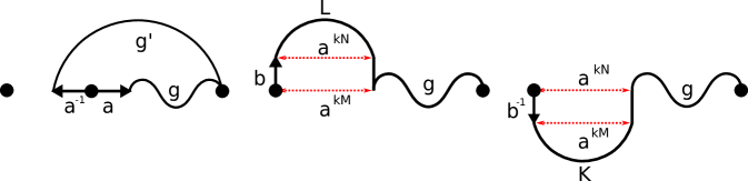
First, we note that the set is closed by prepending and appending the generator and . We factor recursively by considering the first letter in any word (see Figure 1). This gives four cases:
-
•
is the empty word.
-
•
The first letter is or . Then or for some , increasing the length by and altering the -exponent by . At the level of generating functions this gives .
-
•
The first letter is . Factor where is the shortest word so that . Thus, for some . The minimality of ensures . Combined, this gives . At the level of generating functions, the maps words counted by to and resulting in .
-
•
The first letter is . Factor where is the shortest word so that . As per the previous case, for some with . Combined, this gives . Similar reasoning gives
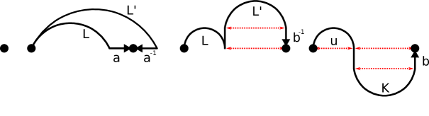
Now consider an element , and we note that (and ) is closed under appending the generators and , but not prepending. See Figure 2. In a similar manner to the above, we factor words in recursively by considering the last letter of .
-
•
is the empty word.
-
•
The last letter is or . Then or for some , increasing the length by and altering the -exponent by . This yields the term .
-
•
The last letter is . Factor where is the longest subword such that and is non-empty. This forces with the restriction that . Since both we must have and , and this yields .
-
•
The last letter is . Factor where is the longest subword such that and is non-empty. This forces with the restriction that . Further, implies the subword . Otherwise, as the subword generates an element with normal form for some .
The generating function for is given by , and so this last case gives .
Putting all of these cases together and rearranging gives the result. The equation for follows a similar argument. ∎
3.2. Solution for
The number of trivial words of length in has long been known to be (for even )333Perhaps the easiest proof known to the authors is the following. Map any trivial word to a path on the square grid. Now rotate the grid and rescale (by ). Each step now changes the -ordinate by and similarly each -ordinate by . In a path of -steps, steps must increase the -ordinate and must decrease it and so giving possibilities. The same occurs independently for the -ordinates and so we get possible trivial words. . This number grows as , and the factor of implies that the corresponding generating function is not algebraic (see, for example, section VII.7 of [23]). The generating function does satisfy a linear differential equation with polynomial coefficients and so is D-finite [43] (in fact it can be written in closed form in terms of elliptic integrals). The class of D-finite functions includes rational and algebraic functions and many of the most famous functions in mathematics and physics. Indeed, most of the known group growth and cogrowth series are D-finite (being algebraic or rational444Kouksov proved that the cogrowth series is a rational function if and only if the group is finite [32].). We prove (below) that when , the cogrowth series is D-finite and we strongly suspect that when , the cogrowth series lies outside this class.
Proposition 3.2.
When the generating functions and the generating functions satisfy
Further, these equations reduce to a set of algebraic equations in and . In particular if we write , and let then we have
For example, for the generating function satisfies the following cubic equation
| (3.3) |
where we have written .
Proof.
The proof is a corollary of Proposition 3.1. Setting simplifies the equations considerably and forces . We note that and the equation for follows. Hence both and are also algebraic. ∎
We are not interested in the full generating function , rather we are mainly interested in the coefficient of .
Corollary 3.3.
For the generating function is D-finite. That is, it satisfies a linear generating function with polynomial coefficients. Furthermore, the cogrowth series (being the generating function of freely reduced words equivalent to the identity) is also D-finite.
It follows that the cogrowth of is an algebraic number.
Proof.
Every algebraic power series also satisfies a linear differential equation with polynomial coefficients (see [43] for many basic facts about D-finite series). It is known [35] that the constant term of a D-finite series of two variables is a D-finite series of a single variable. Substituting an algebraic series into a D-finite series gives another D-finite series, and so transforming from to the cogrowth series (which is done by substituting a rational function) yields another D-finite series.
Finally, if a function satisfies a linear differential equation, then its singularities must correspond to zeros of the coefficient of the highest order derivative. Since the cogrowth series is D-finite, its singularities must be the zeros of the polynomial coefficient of the highest order derivative. ∎
While the results used to prove the above corollary guarantee the existence of such differential equations, they do not give recipes for determining them. There has been a small industry in developing algorithms to do exactly this task (and many other operations on D-finite series) — for example work by Zeilberger, Chyzak and others. Here we have used recent algorithms developed by Chen, Kauers and Singer [11], and we are grateful for Manuel Kauers’ help in the application of these tools.
Applying the algorithms described in [11] to the generating function for which is the solution of equation (3.3) we found a order linear differential equation satisfied by . Unfortunately the polynomial coefficients of this equation have degrees up to 47. We were also able to guess slightly more appealing equations of higher order with lower degree coefficients, but all are too large to list here.
For and we obtain the following equations for (where )
| (3.4) |
and
| (3.5) |
Again applying the same methods, we found an ODE of order 8 with coefficients of degree up to 105 for and for it is order 10 with coefficients of degree up to 154. Using clever guessing techniques (see [31] for a description) Kauers also found DEs for . For the DE is order 12 with coefficients of degree up to 301. While that of took about 50 days of computer time to guess and is 22nd order with coefficients of degree up to 1153; when written in text file is over 6 Mb! We note that the ODEs found for have been proved, but it is beyond current techniques555While there is no theoretical barrier, the time taken by the computations seems to grow quickly with and exceed the available time. to prove those found for higher .
Clearly this approach is not a practical means to study the cogrowth for larger — though one can generate series expansions quite quickly using a computer. We are able to determine the radius of convergence of for much higher via the following lemma.
Lemma 3.4.
For , the generating functions and have the same radius of convergence.
Proof.
We start with some notation. Write
| (3.6) |
Note that we have and that for . Write and . Since all the are non-negative, we immediately have .
To prove the reverse inequality we use a “most popular” argument that is commonly used in statistical mechanics to prove equalities of free-energies (see [29] for example). Fix , then there exists (depending on ) so that — the number is the “most popular” -exponent in all the trivial words of length contributing to the generating function . We have
| (3.7) |
And hence . Note that numerical experiments show that — the distribution is tightly peaked around 0.
Keeping fixed, consider a word that contributes to and another that contributes to . Concatenating them together gives a word that contributes to . So considering all possible concatenation of such pairs of words gives the following inequality
| (3.8) | ||||
| Raise both sides to the power and let gives | ||||
| (3.9) | ||||
Letting then shows that . ∎
We have observed that the statement of the lemma appears to hold for Baumslag-Solitar groups for also, however the above proof breaks down in the general case as the number of summands in equation (3.7) grows exponentially with rather than linearly.
Combining Proposition 3.2 and the above lemma we can establish the growth rates of trivial words and the corresponding cogrowths for the first few values of (see Table 1). Unfortunately we have not been able to find a general form for these numbers. Some simple numerical analysis of these numbers suggests that the growth rate approaches exponentially with increasing . This finding agrees with work of Guyot and Stalder [28], discussed below, who examined the limit of the marked groups as , and found that the groups tend towards the free group on two letters, which has an asymptotic cogrowth rate of .
| 1 | 4 | 3 |
|---|---|---|
| 2 | 3.792765039 | 2.668565568 |
| 3 | 3.647639445 | 2.395062561 |
| 4 | 3.569497357 | 2.215245886 |
| 5 | 3.525816111 | 2.091305394 |
| 6 | 3.500607636 | 2.002421757 |
| 7 | 3.485775158 | 1.936941986 |
| 8 | 3.476962757 | 1.887871818 |
| 9 | 3.471710431 | 1.850717434 |
| 10 | 3.468586539 | 1.822458708 |
We remark that for the number of trivial words is known exactly and hence so is the dominant asymptotic form
In the case of we can show from the differential equations found above that
| for even |
where is given in the previous corollary and we have estimated the amplitudes to be
Unfortunately we have not been able to identify these constants, but these observations lead to the following conjecture.
Conjecture 1.
The number of trivial words in grows as
for .
3.3. Continued fractions and
When we set cancellations occur and the equation for becomes a -deformation of a Catalan generating function:
| (3.10) |
Setting into the first equation reduces it to algebraic and it is readily solved to give which is the generating function of the Catalan numbers. Thus is a -deformation of the Catalan numbers and rearranging the first equation shows that has a simple continued fraction expansion.
| (3.11) |
Such continued fraction forms are well known and understood in Catalan objects (see [22] for example). Unfortunately the equation for does not simplify:
| (3.12) |
Though as noted above and so we expect to be a different -deformation of the Catalan numbers. For we have made even less progress and we have not found , let alone , in closed form. Because of the -deformed nature of we conjecture the following
Conjecture 2.
For Baumslag-Solitar groups with , the generating functions and are not D-finite.
Since any path that contributes to or must also contribute to , it follows that the radius of convergence of is at most — and of course cannot be any smaller. Since the groups are all amenable, we know that . We have been unable to prove any more precise details of the asymptotic form, though it is not unreasonable to expect that
| (3.13) |
While we have been able to generate the first 50-60 terms of the series for by iterating the equations, the series are quite badly behaved and we have been unable to produce reasonable estimates of .
3.4. When
When , we expect that the operators and in the equations satisfied by give rise to -deformations similar to those observed above. In light of this, we extend our previous conjecture:
Conjecture 2 (Extended from the above).
For Baumslag-Solitar groups the generating functions and are only D-finite when .
In spite of the absence of D-finite recurrences, we can still use the equations above to determine the first few terms of the cogrowth series. The resulting algorithm to compute the first terms of the series requires time and memory that are exponential in . The coefficient of is a Laurent polynomial whose degree is exponential in and this exponential growth becomes worse as becomes larger. In spite of this, iteration of these equations to obtain the cogrowth series is exponentially faster than more naive methods based on say a simple backtracking exploration of the Cayley graph, or iteration of the corresponding adjacency matrix.
The time and memory requirements can be further improved since we are primarily interested in the constant term; this means that we do not need to keep high powers of . More precisely if we wish to compute the series to , then we only need to retain those powers of that will contribute to . We must compute the coefficients of for exactly, but we can “trim” subsequent coefficients — the degree of needs only be that of .
Simple c++ code using cln666An open source c++ library for computations with large integers. At time of writing it is available from http://www.ginac.de/CLN/ running on a moderate desktop allowed us to generate about the first 50 terms of for while over 300 terms for were obtained. The series lengths for the other (with ) ranged between these extremes. We have estimated the growth rate of trivial words using differential approximants — see Table 2. Again like the case, we find the series to be very badly behaved (except when ) and we have only obtained quite rough estimates.
| 1 | 2 | 3 | 4 | 5 | |
|---|---|---|---|---|---|
| 1 | 4 | 4 | 4 | 4 | 4 |
| 2 | 3.792765039 | 3.724 | 3.701 | 3.676 | |
| 3 | 3.647639445 | 3.604 | 3.585 | ||
| 4 | 3.569497357 | 3.538 | |||
| 5 | 3.525816111 |
3.5. The limit as
Beautiful work of Luc Guyot and Yves Stalder [28] demonstrates that in the limit as the (marked) group becomes the free group on 2 generators. We note that we can observe this free group behaviour in the functional equations we have obtained.
In particular as , the operators and become the constant-term operators. So in this limit the equations for and from Proposition 3.1 become
| (3.14) |
where and . Clearly and so with a little rearranging
| (3.15) |
Taking the constant term of both sides then gives
| (3.16) |
Simplifying this last expression further gives . The only positive term power series solution of this gives and a similar exercise gives :
| (3.17) |
The expression for is the number of trivial words in the free group on 2 generators.
4. Analysis of random sampling data
4.1. Preliminaries
Using our multiple Markov chain Monte Carlo algorithm we have sampled trivial words from the following groups:
-
•
Baumslag-Solitar groups with
-
•
The basilica group has presentation
(4.1) and embeds in the finitely presented group [27]
(4.2) The groups and are both amenable [5].
We examined two presentations of : The first is obtained from the above by putting , and the second by putting . Simplification gives the representations
(4.3) (4.4) -
•
Other groups for which the cogrowth series is known:
(4.5) -
•
Thompson’s group with the following 3 presentations
(4.6) (4.7) (4.8) Note that the generators above are often called respectively in Thompson’s group literature. We have use some simple Tietze transformations (see [36] p. 89) to obtain the second and third presentations from the first (standard) finite presentation of .
The exact solutions for and are described above, and for the other Baumslag-Solitar groups we have computed series expansions. For the last three groups, the cogrowth series were found by Kouksov [33] and are (respectively)
| (4.9) |
where .
In each case we have obtained estimates of the mean length of freely reduced words as a function of . More precisely, for each group we estimated
| (4.10) |
for and a range of different values and where the sum is over all non-empty freely reduced trivial words. These expectations are dependent on , but one can use Equation (2.22) to form -independent estimates of the canonical expectations. Given a knowledge of the cogrowth series we can quickly compute these same means to any desired precision, since we can also write
| (4.11) |
where is the number of freely reduced words of length . Note that as is increased, the samples are biased towards longer words. This expression is convergent for below the reciprocal of the cogrowth (being the critical point of the associated generating function) and divergent above it. The convergence at the critical point depends on the precise details of the asymptotics of and will be effected by . This then points to a simple way to test for amenability.
Proposition 4.1.
If the mean length of sampled words from a group on generators is finite for slightly above then the group is not amenable.
Note that the amenability or non-amenability of Thompson’s group is an open question, and one that has received an intense amount of interest and study.
4.2. Amenable groups
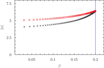
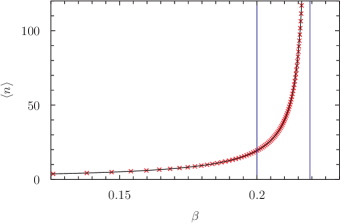
We studied the groups and . The cogrowth series for is known exactly, while we relied on our series expansions to compute statistics for the other two groups — Figure 3 shows the plots of the mean length as a function of .
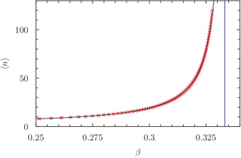
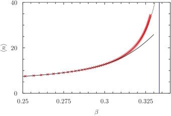
In the case of we see excellent agreement between the numerical estimates generated by our algorithm and the mean length computed from the exact cogrowth series. For and we see good agreement for low between our numerical data and mean length computed from the exact cogrowth series. However at larger values of it appears that the cogrowth series systematically underestimates the mean length, compared to the numerical Monte Carlo data. This is, in fact, due to the modest length of the cogrowth series used to compute mean lengths. For and we were only able to obtain series of length 60 and 56 respectively due to memory constraints. Given longer series we expect much better agreement.
One can, for example, compute longer “approximate” cogrowth series by ignoring small terms. When iterating the functional equations given in Proposition 3.1 one can form reasonable approximations by discarding coefficients which are small compared to nearby coefficients.777Rather than iterating the equations for and then transforming the result to get an approximate cogrowth series, we found that our approximation procedure worked best if we iterated the slightly more complicated equations for the cogrowth series directly — see text following Proposition 3.1 for a description of those equations. More precisely we found that if we discard when , then we obtain good approximations of the cogrowth series. This means that only the large central coefficients are kept and far less memory used. This made it feasible to approximate the cogrowth series out to around 200 or 300 terms. Of course, the results of these approximation should only be considered a rough guide as we have not bounded the size of any resulting errors. That being said, we see very good agreement between these approximations and our numerical data.
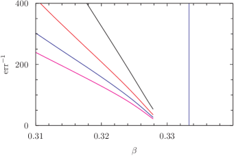
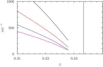
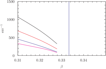
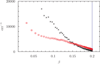
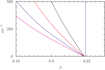
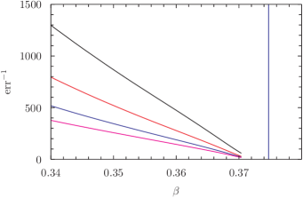
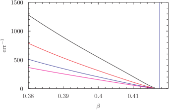
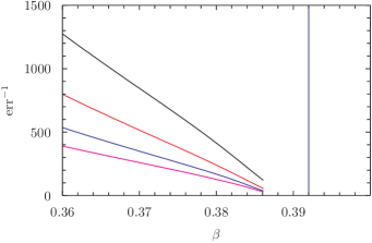
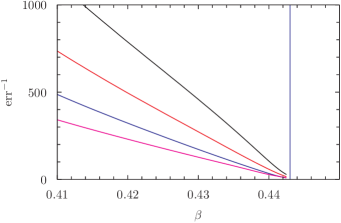
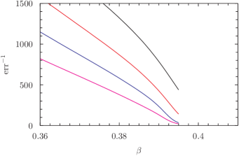
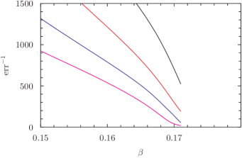
As noted above, we had great difficulty fitting the series data for and . We believe that this is due to the presence of complicated confluent corrections (likely logarithmic terms). Similar corrections also appear to be present in the mean-length data for these groups and we were unable to find convincing or consistent fits to any reasonable functional forms. We did, however, find that the estimated standard error was a good indicator of the location of the singularity: The standard error will diverge as approaches the critical value of . We found that linear or quadratic least squares fits of the reciprocal of the error, and finding their -intercept gave consistent, though perhaps slightly low, estimates of the location of the singularity. See Figure 4. The extrapolations give estimates and for and respectively.
Error bars above were determined by estimating a systematic error in our data. The systematic error was determined by considering the spread of estimates due to our choices of the parameter , the number of data points in the fits, and the chosen functional form for extrapolating the data. We believe that our results give a good indication of quality of the estimates, though we are reluctant to express them as firm confidence intervals. The same general approach to the data for the other groups are followed below.
The HNN-extension of the basilica group were similarly submitted to Monte Carlo simulation by using the representations (4.3) and (4.4). The canonical expected length of the words, , were computed using the ratio estimator (2.22), and turned out to be remarkably insensitive to the parameter (see Figure 5). This made this group more challenging from a numerical perspective than the Baumslag-Solitar groups discussed above. Putting finally gave acceptable results: The sample average length show a divergence close to the critical point (since this group is known to be amenable, this is expected to be at ). As in the case of the Baumslag-Solitar groups, the critical value of was determined by extrapolating the reciprocal of the error. Extrapolating the curve corresponding to representation (4.3) gave and for representation (4.4), . Taking the average and using the absolute difference as a confidence interval gives the estimate to two digits accuracy.
4.3. Non-amenable groups
The groups with and the groups contain a non-abelian free subgroup and so are non-amenable. In the case of the groups and the free subgroups are , and for the free subgroup is .
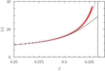
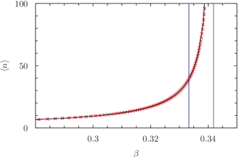
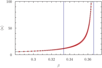
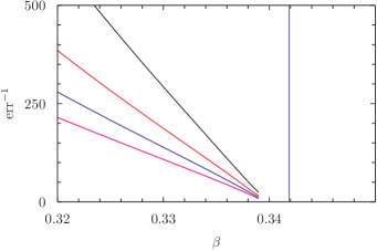
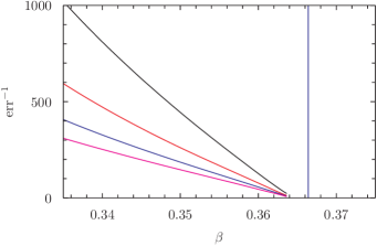
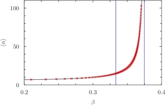
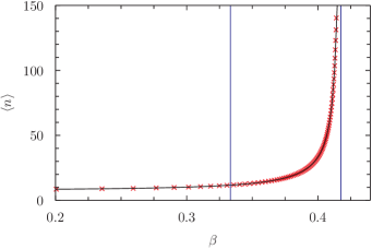
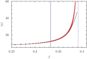
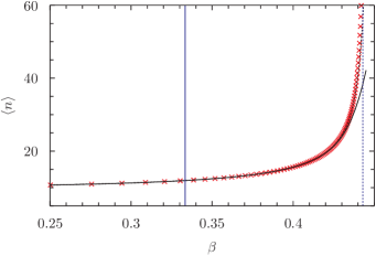
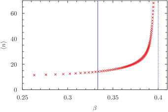
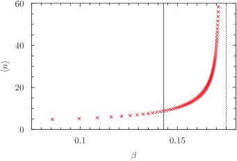
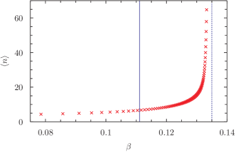
As noted above, the exact cogrowth series is known exactly for Kouksov’s examples and , so we were able to compute the mean length curves exactly — see Figures 6 and 8. As above, we have estimated the location of the dominant singularities for all of these groups — see Figures 7 and 9.
Unfortunately we have been unable to solve and , but we used the recurrences of the previous section to compute the first 100 and 120 terms (respectively) of their cogrowth series. And as was the case for and we also computed an approximation of the cogrowth series using the same method described above. These are plotted against our Monte Carlo data in Figures 10 and 11.
In all cases we see strong agreement between our numerical estimates and the mean length curves computed from series or exact expressions. As was the case with the amenable groups above, fitting the reciprocal of the estimated standard error gives quite acceptable estimates of the location of the dominant singularities and so the cogrowth.
4.4. Thompson’s group
Finally we come to Thompson’s group for which we examine three different presentations as described above. Repeating the same analysis we used on the previous groups we see no evidence of a singularity in the mean length at the amenable values of — see Figures 12 and 13. Indeed our estimates of the location of the dominant singularities are
| (4.12) |
These give cogrowths of and , all of which are well below the amenable values of 3,7 and 9.
5. Conclusions
We have introduced a Markov chain on freely reduced trivial words of any given finitely presented group. The transitions along the chain are defined in terms of conjugations by generators and insertions of relations. These moves are irreducible and satisfy a detailed balance condition; the limiting distribution of the chain is therefore a stretched Boltzmann distribution over trivial words.
In order to validate the algorithm we have implemented it for a range of finitely presented groups for which the cogrowth series is known exactly. We have also added to this set of groups by finding recurrences for the cogrowth series of all Baumslag-Solitar groups. Unfortunately, these recurrences do not have simple closed-form solutions, but can be iterated to obtain far longer series than can be found using brute-force methods. In the case of , the recurrences simplify significantly and we are able to compute the cogrowth exactly. For we have found differential equations satisfied by the cogrowth series which can be used to generate the cogrowth series in polynomial time.
We see excellent agreement between our mean-length estimates and those computed exactly for several groups. As a further check on our simulations, two of the authors independently coded the algorithm and compared the results. We can use our data to estimate the location of the singularity in the generating function of freely reduced trivial words. The location of this singularity is the reciprocal of the cogrowth and so turns out to be an excellent way to predict the amenability of groups. To test this, we used our algorithm on a range of different amenable and non-amenable groups. In each case we found that our numerical estimate of the cogrowth was completely consistent with the known properties of the groups. In particular, where cogrowth is known exactly, our numerics agreed. For each non-amenable group, the numerical “signal” was robust — no evidence of a singularity was seen at the amenable value.
Interestingly, we see no evidence that the mean length of Thompson’s group is divergent close to the amenable value; i.e. for 2,4 and 5 generator presentations we see no evidence of a singularity at or (respectively). Indeed, in each case, the mean length appears to be very smooth for -values some reasonable distance above these points. Varying or examining other statistics does not result in any substantial change with the result that values of consistent with amenability are excluded from our estimated error bars. Overall, our numerical data appears to suggest that Thompson’s group is not amenable. However, the question of the amenability of this group have proven to be particularly subtle, so one way to interpret our data is to say that if is indeed amenable then it is a highly atypical representative in its class.
As an additional note, we have applied our methods to a finitely generated, but not finitely presented amenable group —
| (5.1) |
In this case the algorithm has to be modified slightly. One can no longer choose relations uniformly at random, but instead we choose them from distribution over the relations . As noted in section 2, this distribution must be positive and one must have . With these conditions the algorithm remains ergodic on the space of trivial words and the stationary distribution is still a stretched Boltzmann distribution. This leaves a great deal of freedom in choosing , and our experiments indicated that our results were quite independent of and are consistent with the amenability of the group.
Acknowledgements
The authors thank Manuel Kauers for assistance with establishing the differential equations described in Section 3.2. Similarly we thank Tony Guttmann for discussions on the analysis of series data. Finally we would like to thank Sean Cleary and Stu Whittington for many fruitful discussions.
This research was supported by the Australian Research Council (ARC), the the Natural Sciences and Engineering Research Council of Canada (NSERC), and the Perimeter Institute for Theoretical Physics. Research at Perimeter Institute is supported by the Government of Canada through Industry Canada and by the Province of Ontario through the Ministry of Economic Development and Innovation.

References
- [1] C. Aragão de Carvalho and S. Caracciolo. A new Monte Carlo approach to the critical properties of self-avoiding random walks. J. Physique, 44(3):323–331, 1983.
- [2] C. Aragão de Carvalho, S. Caracciolo, and J. Fröhlich. Polymers and theory in four dimensions. Nuclear Phys. B, 215(2):209–248, 1983.
- [3] Goulnara N. Arzhantseva, Victor S. Guba, Martin Lustig, and Jean-Philippe Préaux. Testing Cayley graph densities. Ann. Math. Blaise Pascal, 15(2):233–286, 2008.
- [4] Laurent Bartholdi, Vadim A. Kaimanovich, and Volodymyr V. Nekrashevych. On amenability of automata groups. Duke Math. J., 154(3):575–598, 2010.
- [5] Laurent Bartholdi and Bálint Virág. Amenability via random walks. Duke Math. J., 130(1):39–56, 2005.
- [6] Laurent Bartholdi and Wolfgang Woess. Spectral computations on lamplighter groups and Diestel-Leader graphs. J. Fourier Anal. Appl., 11(2):175–202, 2005.
- [7] James M. Belk and Kenneth S. Brown. Forest diagrams for elements of Thompson’s group . Internat. J. Algebra Comput., 15(5-6):815–850, 2005.
- [8] R.E. Bellman. Introduction to matrix analysis, volume 19. Society for Industrial Mathematics, 1997.
- [9] B. Berg and D. Foerster. Random paths and random surfaces on a digital computer. Phys. Lett. B, 106(4):323–326, 1981.
- [10] José Burillo, Sean Cleary, and Bert Wiest. Computational explorations in Thompson’s group . In Geometric group theory, Trends Math., pages 21–35. Birkhäuser, Basel, 2007.
- [11] S. Chen, M. Kauers, and M. Singer. Telescopers for rational and algebraic functions via residues. In Proceedings of ISSAC, pages 130–137, 2012. Also preprint arXiv:1201.1954.
- [12] Joel M. Cohen. Cogrowth and amenability of discrete groups. J. Funct. Anal., 48(3):301–309, 1982.
- [13] P.G. De Gennes. Scaling concepts in polymer physics. Cornell Univ Pr, 1979.
- [14] P. Diaconis and L. Saloff-Coste. Moderate growth and random walk on finite groups. Geom. Funct. Anal., 4(1):1–36, 1994.
- [15] P. Diaconis and L. Saloff-Coste. Random walks on finite groups: a survey of analytic techniques. In Probability measures on groups and related structures, XI (Oberwolfach, 1994), pages 44–75. World Sci. Publ., River Edge, NJ, 1995.
- [16] P. Diaconis and L. Saloff-Coste. Walks on generating sets of groups. Invent. Math., 134(2):251–299, 1998.
- [17] Persi Diaconis and Laurent Saloff-Coste. Comparison techniques for random walk on finite groups. Ann. Probab., 21(4):2131–2156, 1993.
- [18] Persi Diaconis and Laurent Saloff-Coste. Comparison theorems for reversible Markov chains. Ann. Appl. Probab., 3(3):696–730, 1993.
- [19] K. Dykema and D. Redelmeier. Lower bounds for the spectral radii of adjacency operators on Baumslag-Solitar groups. Preprint, arXiv:1006.0556, 2010.
- [20] Ken Dykema. Symmetric random walks on certain amalgamated free product groups. In Topological and asymptotic aspects of group theory, volume 394 of Contemp. Math., pages 87–99. Amer. Math. Soc., Providence, RI, 2006.
- [21] Murray Elder, Andrew Rechnitzer, and Thomas Wong. On the cogrowth of Thompson’s group . Groups Complex. Cryptol., 4(2):301–320, 2012.
- [22] P. Flajolet. Combinatorial aspects of continued fractions. Discrete Mathematics, 32(2):125–161, 1980.
- [23] P. Flajolet and R. Sedgewick. Analytic combinatorics. Cambridge Univ Pr, 2009.
- [24] P.J. Flory. Principles of polymer chemistry. Cornell Univ Pr, 1953.
- [25] C.J. Geyer and E.A. Thompson. Annealing Markov chain Monte Carlo with applications to ancestral inference. Journal of the American Statistical Association, pages 909–920, 1995.
- [26] R. I. Grigorchuk. Symmetrical random walks on discrete groups. In Multicomponent random systems, volume 6 of Adv. Probab. Related Topics, pages 285–325. Dekker, New York, 1980.
- [27] R.I. Grigorchuk and Żuk A. On a torsion-free weakly branch group defined by a three state automaton. In International conference on geometric and combinatorial methods in group theory and semigroup theory, volume 12 of Internat. J. Algebra Comput., pages 223–246. World Scientific, Singapore, 2002.
- [28] Luc Guyot and Yves Stalder. Limits of Baumslag-Solitar groups. Groups Geom. Dyn., 2(3):353–381, 2008.
- [29] J.M. Hammersley, G.M. Torrie, and S.G. Whittington. Self-avoiding walks interacting with a surface. Journal of Physics A: Mathematical and General, 15(2):539, 1982.
- [30] EJ Janse van Rensburg. Monte Carlo methods for the self-avoiding walk. Journal of Physics A: Mathematical and Theoretical, 42:323001, 2009.
- [31] M. Kauers. Guessing handbook. Technical report, Johannes Kepler Universität, 2009.
- [32] Dmitri Kouksov. On rationality of the cogrowth series. Proc. Amer. Math. Soc., 126(10):2845–2847, 1998.
- [33] Dmitri Kouksov. Cogrowth series of free products of finite and free groups. Glasg. Math. J., 41(1):19–31, 1999.
- [34] Steven P. Lalley. The weak/strong survival transition on trees and nonamenable graphs. In International Congress of Mathematicians. Vol. III, pages 637–647. Eur. Math. Soc., Zürich, 2006.
- [35] L. Lipshitz. D-finite power series. Journal of Algebra, 122(2):353–373, 1989.
- [36] Roger C. Lyndon and Paul E. Schupp. Combinatorial group theory. Springer-Verlag, Berlin, 1977. Ergebnisse der Mathematik und ihrer Grenzgebiete, Band 89.
- [37] Neal Madras and Gordon Slade. The self-avoiding walk. Probability and its Applications. Birkhäuser Boston Inc., Boston, MA, 1993.
- [38] Avinoam Mann. How groups grow, volume 395 of London Mathematical Society Lecture Note Series. Cambridge University Press, Cambridge, 2012.
- [39] N. Metropolis, A. W. Rosenbluth, M. N. Rosenbluth, A. H. Teller, and E. Teller. Equation of State Calculations by Fast Computing Machines. Journal of Chemical Physics, 21:1087–1092, June 1953.
- [40] Tatiana Nagnibeda. An upper bound for the spectral radius of a random walk on surface groups. Zap. Nauchn. Sem. S.-Peterburg. Otdel. Mat. Inst. Steklov. (POMI), 240(Teor. Predst. Din. Sist. Komb. i Algoritm. Metody. 2):154–165, 293–294, 1997.
- [41] Tatiana Nagnibeda. Random walks, spectral radii, and Ramanujan graphs. In Random walks and geometry, pages 487–500. Walter de Gruyter GmbH & Co. KG, Berlin, 2004.
- [42] Ronald Ortner and Wolfgang Woess. Non-backtracking random walks and cogrowth of graphs. Canad. J. Math., 59(4):828–844, 2007.
- [43] R.P. Stanley. Differentiably finite power series. European J. Combin, 1(2):175–188, 1980.
- [44] Justin Tatch Moore. Fast growth in Folner sets for Thompson’s group , 2009. http://arxiv.org/abs/0905.1118.
- [45] M.C. Tesi, E.J. Janse van Rensburg, E. Orlandini, and S.G. Whittington. Monte Carlo study of the interacting self-avoiding walk model in three dimensions. Journal of Statistical Physics, 82(1):155–181, 1996.
- [46] Stan Wagon. The Banach-Tarski paradox. Cambridge University Press, Cambridge, 1993. With a foreword by Jan Mycielski, Corrected reprint of the 1985 original.
- [47] Wolfgang Woess. Cogrowth of groups and simple random walks. Arch. Math. (Basel), 41(4):363–370, 1983.