Contrasting Multiple Social Network Autocorrelations for Binary Outcomes, With Applications To Technology Adoption

Abstract

The rise of socially targeted marketing suggests that decisions made by consumers can be predicted not only from their personal tastes and characteristics, but also from the decisions of people who are close to them in their networks. One obstacle to consider is that there may be several different measures for “closeness” that are appropriate, either through different types of friendships, or different functions of distance on one kind of friendship, where only a subset of these networks may actually be relevant. Another is that these decisions are often binary and more difficult to model with conventional approaches, both conceptually and computationally. To address these issues, we present a hierarchical model for individual binary outcomes that uses and extends the machinery of the auto-probit method for binary data. We demonstrate the behavior of the parameters estimated by the multiple network-regime auto-probit model (m-NAP) under various sensitivity conditions, such as the impact of the prior distribution and the nature of the structure of the network, and demonstrate on several examples of correlated binary data in networks of interest to Information Systems, including the adoption of Caller Ring-Back Tones, whose use is governed by direct connection but explained by additional network topologies.

1 Introduction

The prevalence and widespread adoption of online social networks have made the analysis of these networks, particularly the behaviors of individuals embedded within, an important topic of study in information systems Agarwal et al. (2008); Oinas-Kukkonen et al. (2010), building off previous work in the context of technology diffusion Brancheau and Wetherbe (1990); Chatterjee and Eliashberg (1990); Premkumar et al. (1994). While past investigations into behavior in networks were typically limited to hundreds of people, contemporary data collection and retrieval technologies enable easy access to network data on a much larger scale. Analyzing the behavior of these individuals, such as their purchasing or technology adoption tendencies, requires statistical techniques that can handle both the scope and the complexity of the data.

The social network aspect is one such complexity. Researchers once assumed that an individual’s decision to purchase a product or adopt a technology is solely associated with their personal attributes, such as age, education, and income Kamakura and Russell (1989); Allenby and Rossi (1998), though this could be due both to a lack of social network data and a mechanism for handling it; indeed, recent developments have shown that their decisions are associated with the decisions of an individual’s neighbors in their social networks Bernheim (1994); Manski (2000); Smith and LeSage (2004). This could be due to a “contagious” effect, where someone imitates the behavior of their friends, or an indication of latent homophily, in which some unobserved and shared trait drives both the tendency for two people to form a friendship and for each to adopt (Aral et al., 2009; Shalizi and Thomas, 2011); either social property will increase the ability to predict a person’s adoption behavior beyond their personal characteristics.

Each of these produces outcomes that are correlated between members of the network who are connected. A popular approach to study this phenomenon is to use a model with explicit autocorrelation between individual outcomes, defined with a single network structure term. With the depth of data now available, an actor is very often observed to be a member of multiple distinct but overlapping networks, such as a friend network, a work colleague network, a family network, and so forth, and each of these networks may have some connection to the outcome of interest, so a model that condenses all networks into one relation will be insufficient. While models have been developed to include two or more network autocorrelation terms, such as Doreian (1989), these do not allow for the immediate and principled inclusion of binary outcomes; other methods to deal with binary outcomes on multiple networks, such as Yang and Allenby (2003), instead take a weighted average of other networks in the system, combining them into one, which has the side effect of constraining the sign of each network autocorrelation component to be identical, which may be undesirable if there are multiple effects thought to be in opposition to one another.

To deal with these issues, we construct a model for binary outcomes that uses the probit framework, allowing us to represent these outcomes as if they are dichotomized outcomes from a multivariate Gaussian random variable; this is then presented as in Doreian (1989) to have multiple regimes of network autocorrelation. We first use the Expectation-Maximization algorithm (EM) to find a maximum likelihood estimator for the model parameters, then use Markov Chain Monte Carlo, a method from Bayesian statistics, to develop an alternate estimate based on the posterior mean. We also study the sensitivity of both solutions to the change of parameters’ prior distribution. Preliminary experiments show that the E-M solution to this model is degenerate, and cannot produce a usable variance-covariance matrix for parameter estimates, and so the MCMC method is preferred. Our software is also validated by using the posterior quantiles method of Cook et al. (2006). We ensure that the parameter estimates from the model are correct by testing first on simulated data, before moving on to real examples of network-correlated behavior.

The rest of the paper is organized as follows. We discuss the literature on the network autocorrelation model in Section 2. Our two estimation algorithms for the multi-network autoprobit, based on EM and MCMC, are presented in Section 3. In Section 4 we present the results of experiments for software validation and parameter estimation behavior observation. Conclusions and suggestions for future work complete the paper in Section 5.

2 Background

[[Previously: Literature]] Network models of behavior are developed to study the process of social influence on the diffusion of a behavior, which is the process “by which an innovation is communicated through certain channels over time among the members of a social system … a special type of communication concerned with the spread of messages that are perceived as new ideas” Rogers (1962). These models have been widely used to study diffusion since the Bass (1969) model, a population-level approach that assumes that everyone in the social network has the same probability of interacting. Such assumption is not realistic because given a large social network, the probability of any random two nodes connecting to each other is not the same; for example, people with closer physical distance communicate more and are likely to exert greater influence on each other. A refinement to this approach is a model where the outcomes of neighboring individuals are explicitly linked, such as the simultaneous autoregressive model (SAR). The general method of SAR is described in Anselin (1988) and Cressie (1993); it considers simultaneous autoregression on the residuals of the form

$$\mathbf{y}=\mathbf{X}\boldsymbol{\beta}+\boldsymbol{\theta},\ \boldsymbol{\theta}=\rho\mathbf{W}\boldsymbol{\theta}+\boldsymbol{\epsilon}$$

where $\mathbf{y}$ is a vector of observed outcomes, in this case consumer choice; $\mathbf{X}$ is a vector of explanatory variables. Rather than an independent error term, $\boldsymbol{\theta}$ represents error terms whose correlation is specified by $\mathbf{W}$, the social network matrix of interest, and $\rho$, the corresponding network autocorrelation, distributing a Gaussian error term $\epsilon_{i}$.

Maximum likelihood estimate solutions are provided by Ord (1975), Doreian (1980, 1982), and Smirnov (2005).

Standard network autocorrelation models can only accommodate one network, such as those of Burt (1987) and Leenders (1997). However, an actor is very often under influence of multiple networks, such as that of friends and that of colleagues. So if a research requires investigation of which autocorrelation term out of multiple networks plays the most significant role in consumers’ decision, none of these models are adequate, and a model that can accommodate two or more networks is necessary.

Cohesion and structural equivalence are two competing social network models to explain diffusion of innovation. In the cohesion model, a focal person’s adoption is influenced by his/her neighbors in the network. In the structural equivalence model, a focal person’s adoption is influenced by the people who have the same position in the social network, such as sharing many common neighbors. While considerable work has been done on these models on real data, the question of which network model best explains diffusion has not been resolved. To approach this, Doreian (1989) introduced a model for “two regimes of network effects autocorrelation” for continuous outcomes. The model is described as below:

$$\mathbf{y}=\mathbf{X}\boldsymbol{\beta}+\rho_{1}\mathbf{W}_{1}\mathbf{y}+\rho_{2}\mathbf{W}_{2}\mathbf{y}+\boldsymbol{\epsilon}$$

where $\mathbf{y}$ is the dependent variable; $\mathbf{X}$ is a vector of explanatory variables; each $\mathbf{W}$ represents a social structure underlying each autoregressive regime. This model takes both interdependence of actors and their attributes, such as demographics, into consideration; these interdependencies are each described by a weight matrix $\mathbf{W}_{i}$. Doreian’s model can capture both actor’s intrinsic opinion and influence from alters in his social network.

As this model takes a continuous dependent variable, Fujimoto and Valente (2011) present a plausible solution for binary outcomes by directly inserting an autocorrelation term $\mathbf{Wy}$ into the right hand side of a logistic regression:

$$y_{i} \sim\operatorname{Be}(p_{i})$$

$$\log(\frac{p_{i}}{1-p_{i}}) =\mathbf{X}\boldsymbol{\beta}+\rho\sum_{j}\mathbf{W}_{ij}\mathbf{y}_{j}$$

Due to its speed of implementation, this method is called “quick and dirty” (QAD) by Doreian (1982). Although it may support a binary dependent variable and multiple network terms, this model does not satisfy the assumption of logistic regression – the observations are not conditionally independent, and the estimation results are biased. Thomas (2012) shows that this method has more consequences than expected for the estimation procedure beyond simple bias; for example, in cases where $\mathbf{W}$ is a directed graph, networks that are directional cannot be distinguished from their reversed counterparts.

Yang and Allenby (2003) propose a hierarchical Bayesian autoregressive mixture model to analyze the effect of multiple network autocorrelation terms on a binary outcome. Their model can only technically accommodate one network effect, composed of several smaller networks that are weighted and added together. This model therefore assumes that all component network coefficients must have the same sign, and also be statistically significant or insignificant together. Such assumptions do not hold if the effect of any but not all of the component networks is statistically insignificant, or of the opposite sign to the other networks, so a method that estimates coefficients for each $\mathbf{W}$ separately is necessary for our applications. We contrast our method with the Yang-Allenby grand $\mathbf{W}$ construction method, a finite mixture of coefficient matrices, in Appendix A.5.

3 Method

We propose a variant of the auto-probit model that accommodates multiple regimes of network autocorrelation terms for the same group of actors, which we call the multiple network auto-probit model (m-NAP). We then provide two methods to obtain estimates for our model. The first is the use of Expectation-Maximization, which employs a maximum likelihood approach, and the second one is a Markov Chain Monte Carlo routine that treats the model as Bayesian. Detailed descriptions of both estimations are shown in Appendix A.1 and A.2.

3.1 Model Specification

The actors are assumed to have $k$ different types of network connections between them, where $\mathbf{W}_{i}$ is the $i^{th}$ network in question $i\in\{1,...,k\}$. $\mathbf{y}$ is the vector of length $n$ of observed binary choices, and is an indicator function of the latent preference of consumers $\mathbf{z}$. If $\mathbf{z}$ is larger than a threshold 0, consumers choose $\mathbf{y}$ as 1; if $\mathbf{z}$ is smaller than 0, then consumers would choose $\mathbf{y}$ as 0.

$$\mathbf{y} =\mathbb{I}(\mathbf{z}>0)$$

$$\mathbf{z} =\mathbf{X}\boldsymbol{\beta}+\boldsymbol{\theta}+\boldsymbol{\epsilon},\ \boldsymbol{\epsilon}\sim\operatorname{Normal}_{n}(0,I_{n})$$

$$\boldsymbol{\theta} =\sum_{i=1}^{k}\rho_{i}\mathbf{W}_{i}\boldsymbol{\theta}+\mathbf{u},\ \mathbf{u}\sim\operatorname{Normal}_{n}(0,\sigma^{2}I_{n})$$

$\mathbf{z}$ is a function of both exogenous covariates $\mathbf{X}$, autocorrelation term $\boldsymbol{\theta}$, and individual error. $\mathbf{X}$ is an $n\times m$ covariate matrixthat includes a constant as its first column; these covariates could be the exogenous characteristics of consumers. $\boldsymbol{\beta}$ is an $m\times 1$ coefficient vector associated with $\mathbf{X}$. $\boldsymbol{\theta}$ is the autocorrelation term, which is responsible for those nonzero covariances in the $\mathbf{z}$. $\boldsymbol{\theta}$ can be described as the aggregation of multiple network structure $\mathbf{W}_{i}$ and coefficient $\rho_{i}$. Each $\mathbf{W}_{i}$ is a network structure describing connections and relationships among consumers.

Our model explicitly allows multiple competing networks that can be defined by different mechanisms on an existing basis of network ties; for example, $\mathbf{W}_{1}$ describes an effect acting directly on a declared tie, such as homophily or social influence, whereas $\mathbf{W}_{2}$ describes the structural equivalence due to those ties. It can also be that each $\mathbf{W}_{i}$ is defined by a different type of network edge, such as friendship, colleagueship, or mutual group membership; note that none of these relationships must be mutually exclusive. Each coefficient $\rho_{i}$ describes the effect size of its corresponding network $\mathbf{W}_{i}$,so that we can compare the relative scales of competing network structures for the same group of actors embedded in social networks.

The error term for the model is modeled as an augmented expression that consists of two parts, $\boldsymbol{\epsilon}$ and $\mathbf{u}$. $\boldsymbol{\epsilon}$ is the unobservable error term of $\mathbf{z}$ that describes individual-level variation that is not shared on the network, and $\mathbf{u}$ is the error that is then distributed along each network, accounting for the non-zero covariance between units. If we marginalize this model by integrating out $\boldsymbol{\theta}$, all the unobserved interdependency will be isolated in a single expression for the distribution of $\mathbf{z}$, given parameters $\boldsymbol{\beta}$, $\rho$ and $\sigma^{2}$, as multivariate with mean $\mathbf{X}\boldsymbol{\beta}$ and variance $\mathbf{Q}$.

$$\mathbf{z} \sim\operatorname{Normal}\left(\mathbf{X}\boldsymbol{\beta},\mathbf{Q}\right)$$

where

$$\mathbf{Q}=I_{n}+\sigma^{2}\left(I_{n}-\displaystyle{\sum_{i=1}^{k}}\rho_{i}\mathbf{W}_{i}\right)^{-1}\left(\left(I_{n}-\displaystyle{\sum_{i=1}^{k}}\rho_{i}\mathbf{W}_{i}\right)^{-1}\right)^{\top}.$$

The non-standard form of the covariance matrix can therefore pose a significant computational issue.

3.2 Expectation-Maximization Solution

We first develop an approach by maximizing the likelihood of the model using E-M. Since $\mathbf{z}$ is latent, we treat it as unobservable data, for which the E-M algorithm is one of the most used methods. Detailed description of our solution for $k$ regimes of network autocorrelation is in Appendix A.1.

The method consists of two steps: first, estimate the expected value of functions of the unobserved $\mathbf{z}$ given the current parameter set $\boldsymbol{\phi}$, $(\boldsymbol{\phi}=\{\boldsymbol{\beta},\boldsymbol{\rho},\sigma^{2}\})$. Second, use these estimates to form a complete data set $\{\mathbf{y},\mathbf{X},\mathbf{z}\}$, with which we estimate a new $\boldsymbol{\phi}$ by maximizing the expectation of the likelihood of the complete data.

We first initialize the parameters to be estimated,

$$\beta_{i} \sim\operatorname{Normal}(\nu_{\beta},\Omega_{\beta});$$

$$\rho_{j} \sim\operatorname{Normal}(\nu_{\rho},\Omega_{\rho});$$

$$\sigma^{2} \sim\operatorname{Gamma}(a,b)$$

where $i=1,...,m$, and $j=1,...,k$. Let these values equal $\boldsymbol{\phi}^{(0)}$.

For the E-step, we calculate the conditional expectation of the log-likelihood, with respect to the augmented data,

$$G(\boldsymbol{\phi}\mid\boldsymbol{\phi}^{(t)}) =\operatorname{E}_{\mathbf{z}\|\mathbf{y},\boldsymbol{\phi}^{(t)}}[\operatorname{log}L(\boldsymbol{\phi}\mid\mathbf{z,y})]$$

$$=-\frac{n}{2}\operatorname{log}2\pi-\frac{n}{2}\operatorname{log}\mid\mathbf{Q}\mid-\frac{1}{2}\sum_{i=1}^{n}\sum_{j=1}^{n}\check{q}_{ij}(\operatorname{E}[z_{i}z_{j}]-\operatorname{E}[z_{i}]X_{j}\beta-\operatorname{E}[z_{j}]X_{i}\beta+X_{i}X_{j}\beta^{2})$$

where $t$ is the current step number and $\check{q}_{ij}$ is element $(i,j)$ in the matrix $\mathbf{Q}^{-1}$.

In the M-step, we maximize $G(\boldsymbol{\phi}\mid\boldsymbol{\phi}^{(t)})$ to get $\boldsymbol{\beta}^{t+1}$, $\boldsymbol{\rho}^{t+1}$ and $[\sigma^{2}]^{(t+1)}$ for the next step.

$$\boldsymbol{\beta}^{(t+1)} =\underset{\boldsymbol{\boldsymbol{\beta}}}{\operatorname{arg\,max}}\ G(\boldsymbol{\beta}\mid\boldsymbol{\rho}^{(t)},\boldsymbol{[\sigma^{2}]}^{(t)});$$

$$\boldsymbol{\rho}^{(t+1)} =\underset{\boldsymbol{\rho}}{\operatorname{arg\,max}}\ G(\boldsymbol{\rho}\mid\boldsymbol{\beta}^{(t+1)},\boldsymbol{[\sigma^{2}]}^{(t)});$$

$$\boldsymbol{[\sigma^{2}]}^{(t+1)} =\underset{[\sigma^{2}]}{\operatorname{arg\,max}}\ G(\boldsymbol{[\sigma^{2}]}\mid\boldsymbol{\beta}^{(t+1)},\boldsymbol{\rho}^{(t+1)})$$

We replace $\boldsymbol{\phi}^{(t)}$ with $\boldsymbol{\phi}^{(t+1)}$ and repeat the E-step and M-step until all the parameters converge. Parameter estimates from the E-M algorithm converge to the MLE estimates Wu (1983).

It is worth noting that the analytical solution for all the parameters is not always possible. Consider the maximization with respect to the autocorrelation variance parameter $\sigma^{2}$:

$$[\sigma^{2}]^{(t+1)} =\underset{[\sigma^{2}]}{\operatorname{arg\,max}}\ G(\boldsymbol{\phi}\mid\boldsymbol{\phi}^{(t)})$$

$$\frac{\partial\operatorname{log}L}{\partial[\sigma^{2}]} =\frac{\partial}{\partial[\sigma^{2}]}\left(-\frac{1}{2}\operatorname{log}\mid\mathbf{Q}\mid-\displaystyle{\frac{1}{2}}(\mathbf{z}-\mathbf{X}\boldsymbol{\beta})^{\top}\mathbf{Q}^{-1}(\mathbf{z}-\mathbf{X}\boldsymbol{\beta})\right)$$ (1)

The first term at the the right hand side of Equation (1) is:

$$\frac{\partial}{\partial[\sigma^{2}]}\operatorname{log}\mid\mathbf{Q}\mid =\frac{\partial}{\partial[\sigma^{2}]}\operatorname{log}\left|I_{n}+[\sigma^{2}]\left(I_{n}-\sum_{i=1}^{k}\rho_{i}\mathbf{W}_{i}\right)^{-1}\left(\left(I_{n}-\sum_{i=1}^{k}\rho_{i}\mathbf{W}_{i}\right)^{-1}\right)^{\top}\right|$$

The second term is:

$$\frac{\partial}{\partial[\sigma^{2}]}(\mathbf{z}-\mathbf{X}\boldsymbol{\beta})^{\top}\mathbf{Q}^{-1}(\mathbf{z}-\mathbf{X}\boldsymbol{\beta})$$

$$=\frac{\partial}{\partial[\sigma^{2}]}(\mathbf{z}-\mathbf{X}\boldsymbol{\beta})^{\top}\left(I_{n}+[\sigma^{2}]\left(I_{n}-\sum_{i=1}^{k}\rho_{i}W_{i}\right)^{-1}\left(\left(I_{n}-\sum_{i=1}^{k}\rho_{i}W_{i}\right)^{-1}\right)^{\top}\right)^{-1}(\mathbf{z}-\mathbf{X}\boldsymbol{\beta})$$

This is not solvable analytically, and numerical methods are needed to get the estimators for this parameter and for $\rho$.

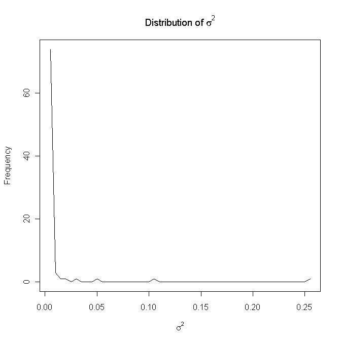
As it happens, the E-M algorithm produces a degenerate solution. This is because it estimates the mode of $\sigma^{2}$, the error term of the autocorrelation term $\theta$, which is at 0 (see Figure 1), and produces a singular variance-covariance matrix estimate using the Hessian approximation. Thus we have to find another solution.

Figure 1: An estimated probability distribution for $\sigma^{2}$, variance of $\boldsymbol{\theta}$. Maximum likelihood methods, such as the Expectation-Maximization method, will choose $\sigma^{2}=0$, a degenerate solution.

3.3 Full Bayesian Solution

We turn to Bayesian methods. Since the observed choice of consumer’s is decided by his/her unobserved preference, this model has a hierarchical structure, so it is natural to think of using a hierarchical Bayesian method. In addition to the model specification above, prior distributions for each of the highest-level parameters in the model are also required. As before, $\mathbf{y}$ is the observed dichotomous choice and calculated by the latent preference $\mathbf{z}$. With Markov Chain Monte Carlo, we generate draws from a series of full conditional probability distributions, derived from the joint distribution. We summarize the forms of the full conditional distributions of all the parameters to estimate in Table 1, and in full in Appendix A.2.

Table 1: Cyclical conditional sampling steps for Markov Chain Monte Carlo

Parameter	Density	Draw Type
$\mathbf{z}$	$\operatorname{TrunNormal}_{n}(\mathbf{X}\boldsymbol{\beta}+\boldsymbol{\theta},I_{n})$	Parallel
$\boldsymbol{\beta}$	$\operatorname{Normal}_{n}(\boldsymbol{\nu}_{\beta},\boldsymbol{\Omega}_{\beta})$	Parallel
$\boldsymbol{\theta}$	$\operatorname{Normal}_{n}(\boldsymbol{\nu}_{\theta},\boldsymbol{\Omega}_{\theta})$	Parallel
$\sigma^{2}$	$\operatorname{InvGamma}(a,b)$	Single
$\rho_{i}$	Metropolis step	Sequential

Given the observed choice of consumer, the latent variable $\mathbf{z}$ is generated from a truncated normal distribution with a mean of $\mathbf{X}\boldsymbol{\beta}+\boldsymbol{\theta}$ with unit error. The prior distributions of the parameters (shown in Table 1 are adapted from priors proposed by Smith and LeSage (2004):

• $\boldsymbol{\beta}$ follows a multivariate normal distribution with mean $\boldsymbol{\nu}_{\beta}$ and variance $\boldsymbol{\Omega}_{\beta}$.

• $\sigma^{2}$ follows an inverse gamma distribution with parameters $a$ and $b$.

• Each $\rho_{i}$ follows a normal distribution with mean $\nu_{\rho}$ and variance $\Omega_{\rho}$.

The sampler algorithm was constructed in the R programming language, including a mechanism to generate data from the model. Validation of the algorithm was conducted using the method of posterior quantiles (Cook et al., 2006), ensuring the correctness of the code for all analyses. Posterior quantiles is a simulation-based method that generates data from the model and verifies that the software can generate parameter estimate randomly around true parameter. For detailed description of the implementation, please see Appendix A.3.

3.4 Sensitivity to Prior Specification

We test the performance of the sampler using prior distributions that are closer to our chosen model than the trivial priors used to check the model code in order to assess the behavior of the algorithm under non-ideal conditions. We demonstrate on data simulated from the model, using two pre-existing network configurations, and specify different prior distributions for each parameter. To demonstrate, we choose a prior distribution for $\rho_{1}$ with high variance, $\rho\sim\operatorname{Normal}(0,100)$, . As shown in Figure 2(a), the posterior draws of $\rho_{1}$ have high temporal autocorrelation. To compare, we choose a narrow prior distribution for $\rho_{1}$, $\rho_{1}\sim\operatorname{Normal}(0.05,0.05^{2})$; the posterior draws for $\rho_{1}$ are shown in Figure 2(b), and the temporal autocorrelation is considerably smaller. With the volume of data under consideration, it is clear that the posterior distribution of $\rho$ is sensitive to its prior distribution.

(a) $\rho\sim\operatorname{Normal}(0,100)$

(b) $\rho\sim\operatorname{Normal}(0.05,0.05^{2})$

Figure 2: Testing the sensitivity of the inference of an autocorrelation parameter $\rho_{1}$ to the prior distribution. (a) The Markov Chain for a weakly informative prior distribution is consistent with the “oracle” value $\rho_{1}$, but the chain has significant temporal autocorrelation. (b) The Markov Chain with a strongly informative prior distribution has much less temporal autocorrelation, but is beholden to its prior distribution more than the data.

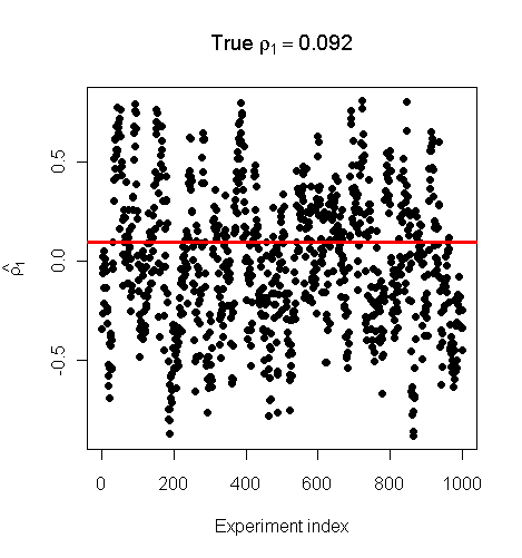
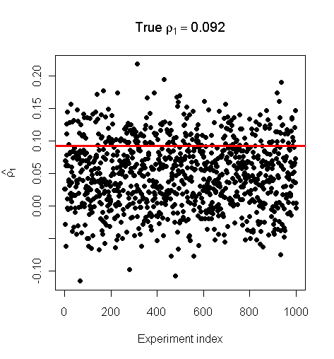
In most of our examples, we do not have a great deal of prior information available on any network parameters, suggesting that most of our analyses will be conducted with minimally informative prior distributions. With such high autocorrelation between sequential draws, the effective sample size is extremely small. We therefore use a high degree of thinning to produce a series of uncorrelated draws from the posterior.

4 Applications

4.1 Auto Purchase Data of Yang and Allenby (2003)

We use Yang and Allenby’s 2003 Japanese car data to compare the findings of our method with those in the original study. The data consists of information on 857 purchase decisions of mid-size cars; the dependent variable is whether the car purchased was Japanese ($y_{m}=1$) or otherwise ($y_{m}=0$). All the car models in the data are substitutable and have roughly similar prices.

An important question of interest is whether the preferences of Japanese car among consumers are interdependent or not. The interdependence in the network is measured by geographical location, where $W_{ij}=1$, if consumer $i$ and $j$ live in the same zip code, and 0, otherwise. Explanatory variables include actors’ demographic information such as age, annual household income, ethnic group, education and other information such as the price of the car, whether the optional accessories are purchased for the car, latitude and longitude of the actor’s location. To construct a network, Yang and Allenby use whether the consumers’ home address in the same zip code as the indicator of a connection. Thus the network structure $\mathbf{W}$, the cohesion, is the joint membership of same geographic area.

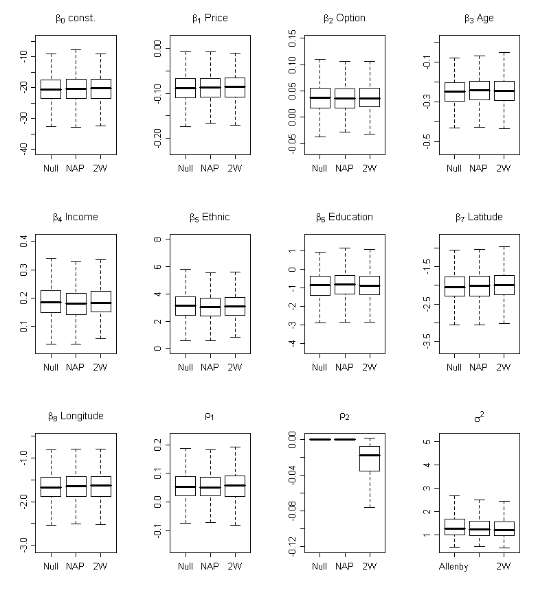
By comparing the parameters of Yang and Allenby’s model to those for m-NAP on the same dataset, with the same underlying definition of network structure, we contrast our approaches and demonstrate the value of separating the impact of various network autocorrelations. The comparison of the coefficient estimates from Yang and Allenby and our Bayesian solution is shown in Figure 3 , for both explanatory variables and for network autocorrelations. We specify a second network term $\mathbf{W}_{2}$ to be the structural equivalence of two consumers, calculated as the simple adjacency distance between the two vectors representing individuals’ connections to other individuals in the network to measure structural equivalence. In a undirected network with non-weighted edges the adjacency distance between two nodes $i$ and $j$ is the number of individuals who have different relationships to $i$ and $j$ respectively,

$$d_{ij} =\sqrt{\sum_{k=1,k\neq i,j}^{N}(A_{ik}-A_{jk})^{2}},$$ (2)

where $A_{ik}=1$ if node $i$ and $k$ are neighbors, and 0 otherwise. The larger $d$ between node $i$ and $j$, the less structurally equivalent they are. We use the inverse of $d_{ij}$ plus one in order to construct a measure with a positive, finite relationship with role equivalence, so that ${s}_{ij}=\frac{1}{d_{ij}+1}$. In our setting, a random element $A_{ij}$ in Equation (2) is from matrix $\mathbf{W}_{1}$, so $d_{ij}$ is the adjacency distance between any two vectors $\textbf{A}_{i}$ and $\textbf{A}_{j}$, representing consumer $i$’s connections, and consumer $j$’s connections to all the other consumers in the data, respectively. The inverse of $d_{ij}$ with an addition to 1 (to avoid zero as denominator), $s_{ij}$, becomes element of structural equivalence matrix $\mathbf{W}_{2}$.

The comparison is shown in Figure 3. Each box contains the estimates of one parameter from three methods: from left to right, Yang and Allenby, NAP with 1 network, and NAP with 2 networks. All the coefficient estimates, $\hat{\boldsymbol{\beta}_{i}}$, $\hat{\boldsymbol{\rho}_{2}}$, and $\hat{\sigma}^{2}$ of the three methods have similar mean, standard deviation and credible interval. One thing interesting here is the effect size of the second network, structural equivalence, has a significant negative effect. This suggests a diminishing cluster effect; when the number of people in the cluster gets bigger, the influence does not increase proportionally.

Figure 3: A comparison of coefficient estimates between the Yang-Allenby method and m-NAP with 1 or 2 networks. The models give similar results, while noting that there is now a negative and statistically significant effect on the network representing structural equivalence. $\beta_{0}$: coefficient of constant term, $\beta_{1}$: coefficient of $\textbf{X}_{1}$, car price; $\beta_{2}$: coefficient of $\textbf{X}_{2}$, car’s optional accessory; $\beta_{3}$: coefficient of $\textbf{X}_{3}$, consumer’s age; $\beta_{4}$: coefficient of $\textbf{X}_{4}$, consumer’s income; $\beta_{5}$: coefficient of $\textbf{X}_{5}$, consumer’s ethnicity; $\beta_{6}$: coefficient of $\textbf{X}_{6}$, residence longitude; $\beta_{7}$: coefficient of $\textbf{X}_{7}$, residence latitude; $\rho_{1}$: coefficient of first network autocorrelation term, $\mathbf{W}_{1}$, cohesion; $\rho_{2}$: coefficient of the second network autocorrelation term, $\mathbf{W}_{2}$, structural equivalence; $\sigma^{2}$: estimated variance of the error term in autocorrelation.

4.2 Caller Ring-Back Tone Usage In A Mobile Network

We use m-NAP to investigate the purchase of Caller Ring Back Tones (CRBT) within a cellular phone network, a technology of increasing interest around the world. When someone calls the subscriber of a CRBT, the caller does not hear the standard ring-back tone but instead hears a song, joke or other message chosen by the subscriber until the subscriber answers the phone or the mailbox takes over. As soon as a CRBT is downloaded, it is set as the default ring back tone, and triggered automatically by all phone call. Our data were obtained from a large Indian telecommunications company (source and raw data confidential). We have cellular phone call records and CRBT purchase records over a three-month period, and phone account holders’ demographic information such as age and gender. We extract a community of 597 users that are highly internally connected from a population with approximately 26 million unique users using the Transitive Clustering and Pruning (T-CLAP) algorithm (Zhang et al., 2011). Within this cluster, network edges are specified between users who call each other during the period of observation, as mutual symmetric connection implies equal and stable relationships (Hanneman and Riddle, 2005), rather than weaker relationships or calls related to businesses (inquiries or telemarketers).

We include several explanatory variables in this model:

• The gender of the cellular phone account holder;

• The age of the account holder;

• The number of unique outbound connections from the user (known as the “outdegree”).

From our original network, we derive two matrices corresponding to cohesion and structural equivalence. Cohesion assumes callers who make phone calls to each other will hear the called party’s CRBT thus more likely to buy that ring-back tone or get interested in CRBT and eventually adopt the technology. Since the number of people a caller calls are drastically different, we normalize the cohesion matrix by dividing each row by the total number of adopters, to make the matrix element to be the percentage of adoption. Structural equivalence is once again defined as the adjacency distance between two callers. Here it is less clear that there is an obvious mechanism for how structural equivalence can impact adoption, as it relates to a relationship that does not expose the caller to the CRBT.

Figure 4: Trace plot of CRBT network parameters. Description of parameters: $\beta_{0}$: coefficient of constant term; $\beta_{1}$: coefficient of consumer’s gender; $\beta_{2}$: coefficient of consumer’s age; $\beta_{3}$: coefficient of number of called contacts; $\rho_{1}$: coefficient of first network autocorrelation term, $\mathbf{W}_{1}$, cohesion; $\rho_{2}$: coefficient of the second network autocorrelation term, $\mathbf{W}_{2}$, structural equivalence; $\sigma^{2}$: estimated variance of the error term in autocorrelation; loglike: log-likelihood of $\mathbf{y}$.

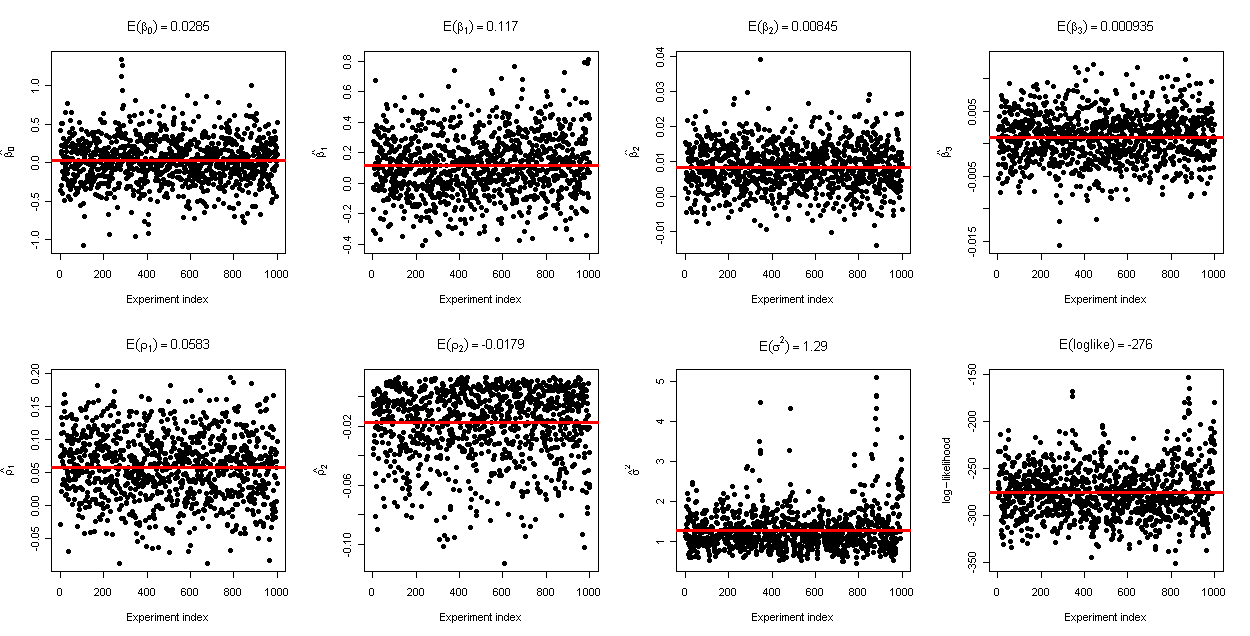
We show estimates for each parameter of the model is shown in Figure 4. Again, we observe a significant negative effect for structural equivalence. This new network autocorrelation, with a coefficient of opposite sign from that of the first network autocorrelation $\mathbf{W}_{1}$, cannot be identified by any earlier models.

5 Conclusion

We have introduced a new auto-probit model to study binary choice of a group of actors that have multiple network relationships among them. We specified the fitting of the model for both E-M and hierarchical Bayesian methods. We found that the E-M solution cannot estimate the parameters for this particular model, thus only hierarchical Bayesian solution can be used here. We also validated our Bayesian solution by using the posterior quantiles method and the results show our software returns accurate estimates. Finally we compare the estimates returned by Yang and Allenby, NAP with one network effect (cohesion), and NAP with two network effects (cohesion and structural equivalence), by using real data.

We want to ensure that the approach can recover variability in the network effect size. Assuming $\mathbf{W}\boldsymbol{\theta}$ has strong effect, we will vary $\rho$’s true value from small number to large number, and observe whether our solution can capture the variation.

Finally we also want to study how multicollinearities between $\mathbf{X}$s, and between $\mathbf{X}$ and $\mathbf{W}\boldsymbol{\theta}$ affect estimated results.

APPENDIX

A.1 E-M solution implementation

A.1.1 Deduction

First, get the distribution of $\boldsymbol{\theta}$.

$$\left(I_{n}-\sum_{i=1}^{k}\rho_{i}\mathbf{W}_{i}\right)\boldsymbol{\theta} =\mathbf{u}$$

$$\boldsymbol{\theta} =\left(I_{n}-\sum_{i=1}^{k}\rho_{i}\mathbf{W}_{i}\right)^{-1}\mathbf{u}$$

$$\boldsymbol{\theta} \sim\operatorname{Normal}\left(0,\sigma^{2}\left(I_{n}-\sum_{i=1}^{k}\rho_{i}\mathbf{W}_{i}\right)^{-1}\left(\left(I_{n}-\sum_{i=1}^{k}\rho_{i}\mathbf{W}_{i}\right)^{-1}\right)^{\top}\right)$$

Then get the distribution of $\mathbf{z}|\boldsymbol{\beta},\boldsymbol{\rho},\sigma^{2}$:

$$\mathbf{z} \sim\operatorname{Normal}\left(\mathbf{X}\boldsymbol{\beta},\mathbf{Q}\right)\text{, where }\mathbf{Q}=I_{n}+\sigma^{2}\left(I_{n}-\sum_{i=1}^{k}\rho_{i}\mathbf{W}_{i}\right)^{-1}\left(\left(I_{n}-\sum_{i=1}^{k}\rho_{i}\mathbf{W}_{i}\right)^{-1}\right)^{\top}$$

The joint distribution of $\mathbf{y}$ and $\mathbf{z}$ can transformed as:

$$p(\mathbf{y}|\mathbf{z})p(\mathbf{z}|\boldsymbol{\beta},\boldsymbol{\rho},\sigma^{2}) =p(\mathbf{y},\mathbf{z}|\boldsymbol{\beta},\boldsymbol{\rho},\sigma^{2})$$

$$=p(\mathbf{z}|\mathbf{y};\boldsymbol{\beta},\boldsymbol{\rho},\sigma^{2})p(\mathbf{y})$$ (3)

The right side of equation (3) are two distributions we already have, as shown below.

$$p(\mathbf{y}) =\displaystyle{\frac{\displaystyle{\frac{1}{\sqrt{2\pi}}}\operatorname{exp}\left(\displaystyle{-\frac{1}{2}}(\mathbf{z}-\mathbf{X}\boldsymbol{\beta})^{\top}(\mathbf{z}-\mathbf{X}\boldsymbol{\beta})\right)}{\Phi(\mathbf{X}\boldsymbol{\beta})}}\mathbb{I}(\mathbf{z}>0)$$

$$\mathbf{z}|\boldsymbol{\beta},\boldsymbol{\rho},\sigma^{2} \sim\operatorname{Normal}(\mathbf{X}\boldsymbol{\beta},\mathbf{Q})$$

$$\mathbf{z}|\mathbf{y},\mathbf{X};\boldsymbol{\beta},\boldsymbol{\rho},\sigma^{2} \sim\operatorname{TrunNormal}(\mathbf{X}\boldsymbol{\beta},\mathbf{Q})$$

Consider parameter $\boldsymbol{\beta}$ only,

$$p(\boldsymbol{\beta},\mathbf{z}|\mathbf{y}) =p(\boldsymbol{\beta}|\mathbf{z},\mathbf{y})p(\mathbf{z}|\mathbf{y})$$

$$\mathbf{z}|\mathbf{y},\mathbf{X};\boldsymbol{\beta} \sim\operatorname{TrunNormal}(\mathbf{X}\boldsymbol{\beta},\mathbf{Q})$$

Assume $\operatorname{Var}(\mathbf{z}$)=1,

$$L(\boldsymbol{\beta}|\mathbf{z}) =\frac{1}{\sqrt{2\pi}}\sum_{i=1}^{n}\operatorname{exp}\left(-\frac{1}{2}(z_{i}-X_{i}\beta)^{2}\right)$$

$$\hat{\boldsymbol{\beta}} =(\mathbf{X}^{\top}\mathbf{X})^{-1}\mathbf{X}^{\top}\mathbf{R},\ \text{where }\mathbf{R}=\operatorname{E}[\mathbf{z}|\boldsymbol{\theta},\mathbf{y}]$$

Then include parameters, $\boldsymbol{\rho}$ and $\sigma^{2}$.

$$\operatorname{E}[\mathbf{z}]^{(t+1)} =\operatorname{E}[\mathbf{z}|\mathbf{y},\boldsymbol{\beta}^{(t)}]=f(\boldsymbol{\beta}^{(t)},\mathbf{y})$$

$$\operatorname{log}L(\boldsymbol{\beta},\boldsymbol{\rho},\sigma^{2}|\mathbf{z}) =\operatorname{log}p(\mathbf{z}|\boldsymbol{\beta},\boldsymbol{\rho},\sigma^{2})$$

$$=\operatorname{log}\prod_{i=1}^{n}p(z_{i}|\boldsymbol{\beta},\boldsymbol{\rho},\sigma^{2})$$

$$=\displaystyle{\sum_{i=1}^{n}}\operatorname{log}\displaystyle{\frac{1}{\sqrt{2\pi|\mathbf{Q}|}}}-\displaystyle{\frac{1}{2}(\mathbf{z}-\mathbf{X}\boldsymbol{\beta})^{\top}\mathbf{Q}^{-1}(\mathbf{z}-\mathbf{X}\boldsymbol{\beta})}$$

$$=\sum_{i=1}^{n}\operatorname{log}\frac{1}{\sqrt{2\pi|\mathbf{Q}|}}-\left(\frac{1}{2}\mathbf{z}^{\top}\mathbf{Q}^{-1}\mathbf{z}-\mathbf{z}^{\top}\mathbf{Q}^{-1}\mathbf{X}\boldsymbol{\beta}-\mathbf{X}^{\top}\boldsymbol{\beta}\mathbf{Q}^{-1}\mathbf{z}+\mathbf{X}^{\top}\boldsymbol{\beta}\mathbf{Q}^{-1}\mathbf{X}\boldsymbol{\beta}\right)$$ (4)

If decompose the matrices above as vector product, then:

(4) $$=\sum_{i=1}^{n}\operatorname{log}\frac{1}{\sqrt{2\pi|\mathbf{Q}|}}-\frac{1}{2}\sum_{i=1}^{n}\sum_{j=1}^{n}(z_{i}-X_{i}\beta)\check{q}_{ij}(z_{j}-X_{j}\beta)$$

$$=\sum_{i=1}^{n}\operatorname{log}\frac{1}{\sqrt{2\pi|\mathbf{Q}|}}-\frac{1}{2}\sum_{i=1}^{n}\sum_{j=1}^{n}\check{q}_{ij}(z_{i}z_{j}-z_{i}X_{j}\beta-z_{j}X_{i}\beta+X_{i}X_{j}\beta^{2})$$

where $\check{q}_{ij}$ is the element in $\check{\mathbf{Q}}$, and $\check{\mathbf{Q}}=\mathbf{Q}^{-1}$.

A.1.2 Expectation step

In the expectation step, get the expected log-likelihood of parameters.

$$Q(\boldsymbol{\phi}|\boldsymbol{\phi}^{(t)}) =\operatorname{E}_{\mathbf{z}|\mathbf{y},\boldsymbol{\phi}^{(t)}}[\operatorname{log}L(\boldsymbol{\phi}|\mathbf{z,y})]$$

$$=\operatorname{E}\left[\sum_{i=1}^{n}\operatorname{log}\frac{1}{\sqrt{2\pi|\mathbf{Q}}}\right]-\operatorname{E}\left[\displaystyle{\frac{1}{2}}(\mathbf{z}-\mathbf{X}\boldsymbol{\beta})^{\top}\mathbf{Q}^{-1}(\mathbf{z}-\mathbf{X}\boldsymbol{\beta})\right]$$

$$=-\frac{n}{2}\operatorname{log}2\pi-\frac{n}{2}\operatorname{log}|\mathbf{Q}|-\frac{1}{2}\sum_{i=1}^{n}\sum_{j=1}^{n}\check{q}_{ij}(\operatorname{E}[z_{i}z_{j}]-\operatorname{E}[z_{i}]X_{j}\beta-\operatorname{E}[z_{j}]X_{i}\beta+X_{i}X_{j}\beta^{2})$$

where $\boldsymbol{\phi}$ is the parameter set, and $t$ is the number of steps.

A.1.3 Maximization step

In the maximization step, get the parameter estimates maximizing the expected log-likelihood. First, estimate $\boldsymbol{\beta}$

$$\boldsymbol{\beta}^{(t+1)} =\underset{\boldsymbol{\boldsymbol{\beta}}}{\operatorname{arg\,max}}\ Q(\boldsymbol{\phi}|\boldsymbol{\phi}^{(t)})$$

$$=\underset{\boldsymbol{\boldsymbol{\beta}}}{\operatorname{arg\,max}}\ \displaystyle{\sum_{i=1}^{n}}\operatorname{log}\displaystyle{\frac{1}{\sqrt{2\pi|\mathbf{Q}|}}}-\displaystyle{\frac{1}{2}}(\mathbf{z}-\mathbf{X}\boldsymbol{\beta})^{\top}\mathbf{Q}^{-1}(\mathbf{z}-\mathbf{X}\boldsymbol{\beta})$$ (5)

If directly apply analytical method to solve the Equation (5) above, then:

$$\frac{\partial\operatorname{log}L}{\partial\boldsymbol{\beta}} =\frac{\partial}{\partial\boldsymbol{\beta}}\left(-\displaystyle{\frac{1}{2}}(\mathbf{z}-\mathbf{X}\boldsymbol{\beta})^{\top}\mathbf{Q}^{-1}(\mathbf{z}-\mathbf{X}\boldsymbol{\beta})\right)$$

$$\frac{\partial}{\partial\boldsymbol{\beta}}(\mathbf{z}-\mathbf{X}\boldsymbol{\beta})^{\top}\mathbf{Q}^{-1}(\mathbf{z}-\mathbf{X}\boldsymbol{\beta}) =\frac{\partial}{\partial\boldsymbol{\beta}}(\mathbf{z}^{\top}\mathbf{Q}^{-1}\mathbf{z}-\mathbf{z}^{\top}\mathbf{Q}^{-1}\mathbf{X}\boldsymbol{\beta}-\boldsymbol{\beta}^{\top}\mathbf{X}^{\top}\mathbf{Q}^{-1}\mathbf{z}+\boldsymbol{\beta}^{\top}\mathbf{X}^{\top}\mathbf{Q}^{-1}\mathbf{X}\boldsymbol{\beta})$$

$$=-\mathbf{z}^{\top}\mathbf{Q}^{-1}\mathbf{X}-\mathbf{X}^{\top}\mathbf{Q}^{-1}\mathbf{z}+\mathbf{X}^{\top}\mathbf{Q}^{-1}\mathbf{X}\boldsymbol{\beta}$$ (6)

Set Equation (6) as 0, then:

$$-\mathbf{z}^{\top}\mathbf{Q}^{-1}\mathbf{X}-\mathbf{X}^{\top}\mathbf{Q}^{-1}\mathbf{z}+\mathbf{X}^{\top}\mathbf{Q}^{-1}\mathbf{X}\boldsymbol{\beta} =0$$

$$\hat{\boldsymbol{\beta}} =\left(\mathbf{X}^{\top}\mathbf{Q}^{-1}\mathbf{X}\right)^{-1}\mathbf{X}^{\top}\mathbf{Q}^{-1}\mathbf{R}$$

Second, estimate parameter $\boldsymbol{\rho}$:

$$\boldsymbol{\rho}^{(t+1)} =\underset{\boldsymbol{\rho}}{\operatorname{arg\,max}}\ Q(\boldsymbol{\phi}|\boldsymbol{\phi}^{(t)})$$

Assume $\boldsymbol{\rho}=\{\rho_{1},...,\rho_{k}\}$, without losing any generalizabiliy, $\rho_{1}$ can be estimated as:

$$\rho_{1}^{(t+1)} =\underset{\rho_{1}}{\operatorname{arg\,max}}\ Q(\boldsymbol{\phi}|\boldsymbol{\phi}^{(t)})$$

$$\frac{\partial\operatorname{log}L}{\partial\rho_{1}} =\frac{\partial}{\partial\rho_{1}}\left(-\frac{1}{2}\operatorname{log}|\mathbf{Q}|-\displaystyle{\frac{1}{2}}(\mathbf{z}-\mathbf{X}\boldsymbol{\beta})^{\top}\mathbf{Q}^{-1}(\mathbf{z}-\mathbf{X}\boldsymbol{\beta})\right)$$

$$\frac{\partial}{\partial\rho_{1}}\operatorname{log}|\mathbf{Q}| =-\operatorname{tr}(\mathbf{W}_{1}\mathbf{Q}^{-1})$$

$$\frac{\partial}{\partial\rho_{1}}(\mathbf{z}-\mathbf{X}\boldsymbol{\beta})^{\top}\mathbf{Q}^{-1}(\mathbf{z}-\mathbf{X}\boldsymbol{\beta}) =\frac{\partial}{\partial\rho_{1}}(\mathbf{z}^{\top}\mathbf{Q}^{-1}\mathbf{z}-\mathbf{z}^{\top}\mathbf{Q}^{-1}\mathbf{X}\boldsymbol{\beta}-\boldsymbol{\beta}^{\top}\mathbf{X}^{\top}\mathbf{Q}^{-1}\mathbf{z}+\boldsymbol{\beta}^{\top}\mathbf{X}^{\top}\mathbf{Q}^{-1}\mathbf{X}\boldsymbol{\beta})$$

It is impossible to get the analytical solution for $\rho_{i}$.

Third, estimate parameter $\sigma^{2}$. Let $\sigma^{2}=[\sigma^{2}]$

$$[\sigma^{2}]^{(t+1)} =\underset{[\sigma^{2}]}{\operatorname{arg\,max}}\ Q(\boldsymbol{\phi}|\boldsymbol{\phi}^{(t)})$$

$$\frac{\partial\operatorname{log}L}{\partial[\sigma^{2}]} =\frac{\partial}{\partial[\sigma^{2}]}\left(-\frac{1}{2}\operatorname{log}|\mathbf{Q}|-\displaystyle{\frac{1}{2}}(\mathbf{z}-\mathbf{X}\boldsymbol{\beta})^{\top}\mathbf{Q}^{-1}(\mathbf{z}-\mathbf{X}\boldsymbol{\beta})\right)$$ (7)

The first term at the the right hand side of equation above is:

$$\frac{\partial}{\partial[\sigma^{2}]}\operatorname{log}|\mathbf{Q}| =\frac{\partial}{\partial[\sigma^{2}]}\operatorname{log}\left|I_{n}+[\sigma^{2}]\left(I_{n}-\sum_{i=1}^{k}\rho_{i}\mathbf{W}_{i}\right)^{-1}\left(\left(I_{n}-\sum_{i=1}^{k}\rho_{i}\mathbf{W}_{i}\right)^{-1}\right)^{\top}\right|$$

The second term is:

$$\frac{\partial}{\partial[\sigma^{2}]}(\mathbf{z}-\mathbf{X}\boldsymbol{\beta})^{\top}\mathbf{Q}^{-1}(\mathbf{z}-\mathbf{X}\boldsymbol{\beta})$$

$$=\frac{\partial}{\partial[\sigma^{2}]}(\mathbf{z}-\mathbf{X}\boldsymbol{\beta})^{\top}\left(I_{n}+[\sigma^{2}]\left(I_{n}-\sum_{i=1}^{k}\rho_{i}W_{i}\right)^{-1}\left(\left(I_{n}-\sum_{i=1}^{k}\rho_{i}W_{i}\right)^{-1}\right)^{\top}\right)^{-1}(\mathbf{z}-\mathbf{X}\boldsymbol{\beta})$$

This is again not solvable by using analytical method.

A.2 Markov Chain Monte Carlo estimation

The Markov Chain Monte Carlo method generates a sequence of draws that approaches the posterior distribution of interest. Our solution consists of steps as follows.

Step 1. Generate $\mathbf{z}$, $\mathbf{z}$ follows truncated normal distribution.

$$\mathbf{z}\sim\operatorname{TrunNormal}_{n}(\mathbf{X}\boldsymbol{\beta}+\boldsymbol{\theta},I_{n})$$

where $I_{n}$ is the $n\times n$ identity matrix. If $y_{i}=1$, then $z_{i}\geq 0$, if $y_{i}=0$, then $z_{i}<0$

Step 2. Generate $\boldsymbol{\beta}$, $\boldsymbol{\beta}\sim\operatorname{Normal}(\boldsymbol{\nu}_{\beta},\boldsymbol{\Omega}_{\beta})$

1. define $\boldsymbol{\beta}_{0}$, where

   $$\boldsymbol{\beta}_{0}=\left[\begin{array}[]{c}0\\ 0\\ \vdots\\ 0\end{array}\right]$$

2. define $\mathbf{D}=hI_{n}$, $\mathbf{D}$ is a baseline variance matrix, corresponding to the prior $p(\boldsymbol{\beta})$, where $h$ is a large constant, e.g. 400.

   $$\mathbf{D}^{-1}=\left[\begin{array}[]{cccc}\sigma_{0}^{2}&0&\ldots&0\\ 0&\sigma_{0}^{2}&\ldots&0\\ \vdots&\vdots&\ldots&\vdots\\ 0&0&\ldots&\sigma_{0}^{2}\end{array}\right]$$

   Set $\sigma_{0}^{2}$ as $\displaystyle{\frac{1}{400}}$, a small number close to 0, compared with $\operatorname{Normal}(0,1)$, where $\sigma_{0}^{2}=1$

3. $\boldsymbol{\Omega}_{\beta}=\left(\mathbf{D}^{-1}+\mathbf{X}^{\top}\mathbf{X}\right)^{-1}$
   This is because:

   $$\mathbf{z} =\mathbf{X}\boldsymbol{\beta}+\boldsymbol{\theta}+\boldsymbol{\epsilon}$$

   $$\boldsymbol{\beta} =\mathbf{X}^{-1}(\mathbf{z}-\boldsymbol{\theta}-\boldsymbol{\epsilon})$$

   $\therefore\boldsymbol{\beta}\sim\operatorname{Normal}\left(\mathbf{X}^{-1}(\mathbf{z}-\boldsymbol{\theta}),\ (\mathbf{X}^{\top}\mathbf{X})^{-1}\right)$
   Based on law of initial values, $\boldsymbol{\Omega}_{\beta}=\left(\mathbf{D}^{-1}+\mathbf{X}^{\top}\mathbf{X}\right)^{-1}$

4. Then $\boldsymbol{\nu}_{\beta}$ can be represented by $\boldsymbol{\nu}_{\beta}=\boldsymbol{\Omega}_{\beta}\left(\mathbf{X}^{\top}(\mathbf{z}-\boldsymbol{\theta})+\mathbf{D}^{-1}\right)$

Step 3. Generate $\boldsymbol{\theta}$, $\boldsymbol{\theta}\sim\operatorname{Normal}(\boldsymbol{\nu}_{\theta},\boldsymbol{\Omega}_{\theta})$

1. First, define $\mathbf{B}=I_{n}-\displaystyle{\sum_{i}}\rho_{i}\mathbf{W}_{i}$

   $$\boldsymbol{\theta} =\displaystyle{\sum_{i}}\rho_{i}\mathbf{W}_{i}+\mathbf{u}$$

   $$(I_{n}-\displaystyle{\sum_{i}}\rho_{i}\mathbf{W}_{i})\boldsymbol{\theta} =\mathbf{u}$$

   $$\mathbf{B}\boldsymbol{\theta} =\mathbf{u}$$

   $$\boldsymbol{\theta} =\mathbf{B}^{-1}\mathbf{u}$$

   Let $\operatorname{Var}(\mathbf{u})=\sigma^{2}I_{n}$

   $$\operatorname{Var}(\boldsymbol{\theta}) =\operatorname{Var}(\mathbf{B}^{-1}\mathbf{u})$$

   $$=(\mathbf{B}^{\top}\mathbf{B})^{-1}\sigma^{2}I_{n}$$

   $$=\left(\displaystyle{\frac{\mathbf{B}^{\top}\mathbf{B}}{\sigma^{2}}}\right)^{-1}$$

2. Then $\boldsymbol{\Omega}_{\theta}=\left(I_{n}+\displaystyle{\frac{\mathbf{B}^{\top}\mathbf{B}}{\sigma^{2}}}\right)^{-1}$ We then add an offset $I_{n}$ to $\displaystyle{\frac{\mathbf{B}^{\top}\mathbf{B}}{\sigma^{2}}}$. So $\boldsymbol{\Omega}_{\theta}=\left(I_{n}+\displaystyle{\frac{\mathbf{B}^{\top}\mathbf{B}}{\sigma^{2}}}\right)^{-1}$

3. $\boldsymbol{\nu}_{\theta}=\boldsymbol{\Omega}_{\theta}(\mathbf{z}-\mathbf{X}\boldsymbol{\beta})$, since $\boldsymbol{\theta}=(\mathbf{z}-\mathbf{X}\boldsymbol{\beta})-\boldsymbol{\epsilon}$

Step 4. Generate $\sigma^{2}$, $\sigma^{2}\sim\operatorname{InvGamma}(a,b)$

$$a =s_{0}+\displaystyle{\frac{n}{2}}$$

$$b =\displaystyle{\frac{2}{\boldsymbol{\theta}^{\top}\mathbf{B}^{\top}\mathbf{B}\boldsymbol{\theta}+\displaystyle{\frac{2}{q_{0}}}}}$$

where $s_{0}$ and $q_{0}$ are the parameters for the conjugate prior of $\sigma^{2}$, and $n$ is the size of data.

Step 5. Finally we generate coefficient for $\mathbf{W}$, $\rho_{i}$, using Metropolis-Hasting sampling with a random walk chain.

$$\rho_{i}^{new}=\rho_{i}^{old}+\Delta_{i},$$

where the increment random variable $\Delta_{i}\sim\operatorname{Normal}(\nu_{\Delta},\Omega_{\Delta})$.

The accepting probability $\alpha$ is obtained by:

$$\operatorname{min}\left(\displaystyle{\frac{|\mathbf{B}_{new}|\operatorname{exp}\left(-\displaystyle{\frac{1}{2\sigma^{2}}}\boldsymbol{\theta}^{\top}\mathbf{B}_{new}^{\top}\mathbf{B}_{new}\boldsymbol{\theta}\right)}{|\mathbf{B}_{old}|\operatorname{exp}\left(-\displaystyle{\frac{1}{2\sigma^{2}}}\boldsymbol{\theta}^{\top}\mathbf{B}_{old}^{\top}\mathbf{B}_{old}\boldsymbol{\theta}\right)}},1\right)$$

A.3 Validation of Bayesian Software

One challenge of Bayesian methods is getting an error-free implementation. Bayesian solutions often have high complexity, and a lack of software causes many researchers to develop their own, greatly increasing the chance of software error; many models are not validated, and many of them have errors and do not return correct estimations. So it is very necessary to confirm that the code returns correct results. The validation of Bayesian software implementations has a short history; we wrote a program using a standard method, the method of posterior quantiles Cook et al. (2006), to validate our software. This method again is a simulation-based method. The idea is to generate data from the model and verify that the software will properly recover the underlying parameters in a principled way. First, we draw the parameters $\theta$ from its prior distribution $p(\Theta)$, then generate data from distribution $p(y\mid\theta)$. If the software is correctly coded, the quantiles of each true parameter should be uniformly distributed with respect to the algorithm output. For example, the $95\%$ credible interval should contain the true parameter with probability $95\%$. Assume we want to estimate the parameter $\theta$ in Bayesian model $p(\theta\mid y)=p(y\mid\theta)p(\theta)$, where $p(\theta)$ is the prior distribution of $\theta$, $p(y\mid\theta)$ is the distribution of data, and $p(\theta\mid y)$ is the posterior distribution. The estimated quantile can be defined as:

$$\hat{q}(\theta_{0})=\hat{P}(\theta<\theta_{0})=\frac{1}{N}\sum_{i=1}^{N}\mathbb{I}(\theta_{i}<\theta_{0})$$

where $\theta_{0}$ is the true value drawn from prior distribution; $\hat{\theta}$ is a series of draw from posterior distribution generated by the software to-be-tested; $N$ is the number of draws in MCMC. The quantile is the probability of posterior sample smaller than the true value, and the estimated quantile is the number of posterior draws generated by software smaller than the true value. If the software is correctly coded, then the quantile distribution for parameter $\theta$, $\hat{q}(\theta_{0})$ should approaches $\operatorname{Uniform}(0,1)$, when $N\rightarrow\infty$ Cook et al. (2006). The whole process up to now is defined as one replication. If run a number of replications, we expect to observe a uniformly distribution $\hat{q}(\theta_{0})$ around $\theta_{0}$, meaning posterior should be randomly distributed around the true value.

We then demonstrate the simulations we ran. Assume the model we want to estimate is:

$$\mathbf{z} =\mathbf{X}_{1}\beta_{1}+\mathbf{X}_{2}\beta_{2}+\boldsymbol{\theta}+\boldsymbol{\epsilon};$$

$$\boldsymbol{\theta} =\rho_{1}\mathbf{W}_{1}\boldsymbol{\theta}+\rho_{2}\mathbf{W}_{2}\boldsymbol{\theta}+\mathbf{u}$$

We then specified a prior distribution for each parameter, and use MCMC to simulate the posterior distributions.

$$\boldsymbol{\beta} \sim\operatorname{Normal}(0,1);$$

$$\sigma^{2} \sim\operatorname{InvGamma}(5,10);$$

$$\boldsymbol{\rho} \sim\operatorname{Normal}(0.05,0.05^{2})$$

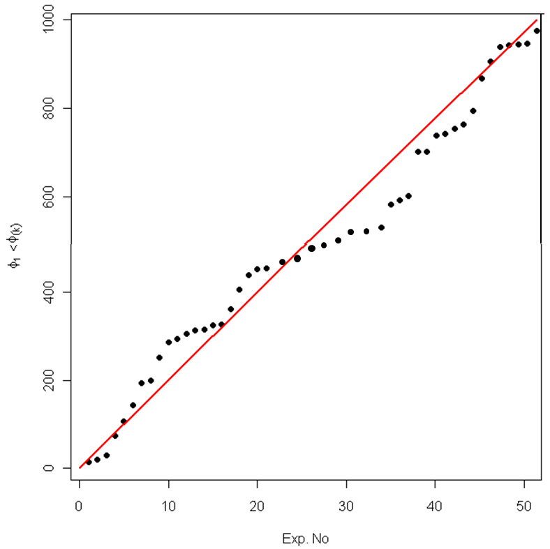
We performed a simulation of 10 replications to validate our hierarchical Bayesian MCMC software. The generated sample size for $\mathbf{X}$ is 50, so the size of the network structure $\mathbf{W}$ is 50 by 50. In each replication we generated 20000 draws from the posterior distribution of all the parameters in $\boldsymbol{\phi}$ ($\boldsymbol{\phi}=\{\beta_{1},\beta_{2},\rho_{1},\rho_{2},\sigma^{2}\}$), and kept one from every 20 draws, yielding 1000 draws for each parameter. We then count the number of draws larger than the true parameters in each replication. If the software is correctly written, each estimated value should be randomly distributed around the true value, so the number of estimates larger than the true value should be uniformly distributed among the 10 replications. We pooled all these quantiles for the five parameters, 50 in total, and the sorted results are shown in Figure 5.

Figure 5: Distribution of sorted quantiles of parameters, $\beta_{1},\beta_{2},\rho_{1},\rho_{2},\sigma^{2}$, over 10 replications. The roughly uniform distribution indicates that the algorithm code functions correctly for data simulated from the model.

A.4 Solution diagnostic

We run MCMC experiment to confirm there is no autocorrelation among draws of each parameter. In this experiment, we set the length of MCMC chain as 30,000, burn-in as 10,000, and thinning as 20, which is used for removing the autocorrelations between draws. The trace plots generated from our code for the 1000 draws after burn-in and thinning are listed in the Figure 6 below.

Figure 6: Trace plot of a two-network auto-probit model. $\beta_{0}$: coefficient of constant term, $\beta_{1}$: coefficient of car price; $\beta_{2}$: coefficient of car’s optional accessory; $\beta_{3}$: coefficient of consumer’s age; $\beta_{4}$: coefficient of consumer’s income; $\beta_{5}$: coefficient of consumer’s ethnicity; $\beta_{6}$: coefficient of residence longitude; $\beta_{7}$: coefficient of residence latitude; $\rho_{1}$: coefficient of first network autocorrelation term, $\mathbf{W}_{1}$, cohesion; $\rho_{2}$: coefficient of the second network autocorrelation term, $\mathbf{W}_{2}$, structural equivalence; $\sigma^{2}$: estimated variance of the error term in autocorrelation.

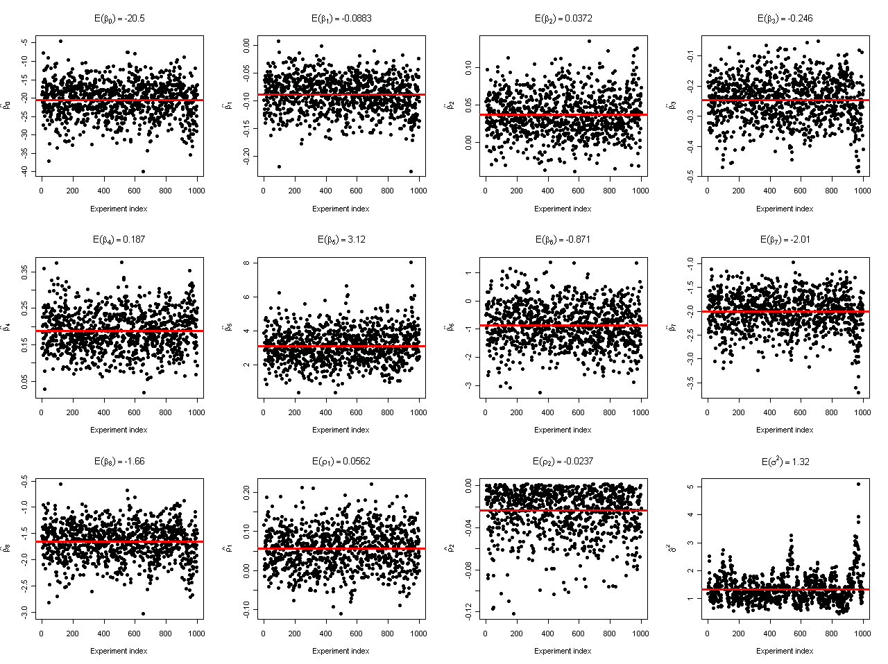
We have 12 plots total. Each plot depicts draws for a particular parameter estimation. The first 9 plots, from left to right and top to bottom, are the trace for the $\beta_{i}$, coefficient of independent variables. Each point represents the value of estimated coefficient $\hat{\beta_{i}}$, and the red line represents the mean. We observe all $\hat{\beta_{i}}$s are randomly distributed around the mean, and the mean is significant, showing the estimation results are valid. The 10th and 11th plots are for the two estimated network effect coefficients $\hat{\rho_{1}}$ and $\hat{\rho_{2}}$. We found both $\hat{\rho_{i}}$ are also significant, and randomly distributed around their means. The only coefficient showing autocorrelation is $\sigma^{2}$.

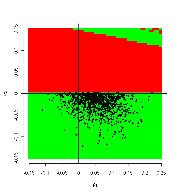
Note that not all values of $\rho_{1}$ and $\rho_{2}$ can make $\mathbf{B}$ ($\mathbf{B}=I_{n}-\rho_{1}\mathbf{W}_{1}-\rho_{2}\mathbf{W}_{2}$) invertible. The plot below shows the relationship between the values of $\rho_{1}$ and $\rho_{2}$, and the invertibility of $\mathbf{B}$. The green area is where $\mathbf{B}$ is invertible, and red area is otherwise. If limit draws to the green area, we will have correlated $\rho_{1}$ and $\rho_{2}$. When we draw $\rho_{1}$ and $\rho_{2}$ using bivariate normal, there is no apparent correlation between them (see Figure 7). We understand the correlation between $\rho_{1}$ and $\rho_{2}$ comes from the definition of $\mathbf{W}_{1}$ and $\mathbf{W}_{2}$, not the prior non-correlation.

Figure 7: Regions of validity for $\rho_{1}$ and $\rho_{2}$ for which $\mathbf{B}$ is invertible (green) or not (red).

A.5 W as a mixture of matrices

Yang and Allenby 2003) specified the autoregressive matrix W as a finite mixture of coefficient matrices, each related to a specific covariate:

$$\mathbf{W}=\sum_{i=1}^{n}\phi_{i}\mathbf{W}_{i}$$

$$\sum_{i=1}^{n}\phi_{i}=1$$

where $i$ represents the indices of the covariates, $i$ = 1… $n$. $\phi_{i}$ is the correspondent weight of the component matrix $\mathbf{W}_{i}$. $\mathbf{W}_{i}$ is associated with a covariate $\textbf{X}_{i}$.

References

- Agarwal et al. (2008) Agarwal, R., Gupta, A. K. and Kraut, R. (2008). Editorial overview – the interplay between digital and social networks. Information Systems Research, 19 243–252.
- Allenby and Rossi (1998) Allenby, G. M. and Rossi, P. E. (1998). Marketing models of consumer heterogeneity. Journal of Econometrics, 89 57–78.
- Anselin (1988) Anselin, L. (1988). Spatial Econometrics: Methods and Models. 1st ed. Studies in Operational Regional Science, Springer, The Netherlands.
- Aral et al. (2009) Aral, S., Muchnik, L. and Sundararajan, A. (2009). Distinguishing Influence Based Contagion from Homophily Driven Diffusion in Dynamic Networks. Proceedings of the National Academy of Sciences, 106 21544.
- Bass (1969) Bass, F. M. (1969). A new product growth for model consumer durables. Management Science, 15 215–227.
- Bernheim (1994) Bernheim, B. D. (1994). A theory of conformity. Journal of Political Economy, 102 841–77.
- Brancheau and Wetherbe (1990) Brancheau, C. J. and Wetherbe, C. J. (1990). The adoption of spreadsheet software: Testing innovation diffusion theory in the context of end-user computing. Information Systems Research, 1 115–143.
- Burt (1987) Burt, R. S. (1987). Social contagion and innovation: Cohesion versus structural equivalence. American Journal of Sociology, 92 1287.
- Chatterjee and Eliashberg (1990) Chatterjee, R. and Eliashberg, J. (1990). The innovation diffusion process in a heterogeneous population: A micromodeling approach. Management Science, 36 1057–1079.
- Cook et al. (2006) Cook, S. R., Gelman, A. and Rubin, D. B. (2006). Validation of software for bayesian models using posterior quantiles. Journal of Computational and Graphical Statistics, 15 675–692.
- Cressie (1993) Cressie, N. A. C. (1993). Statistics for Spatial Data. Revised ed. Probability and Statistics series, Wiley-Interscience, New York.
- Doreian (1980) Doreian, P. (1980). Linear models with spatially distributed data: Spatial disturbances or spatial effects. Sociological Methods and Research, 9 29–60.
- Doreian (1982) Doreian, P. (1982). Maximum likelihood methods for linear models: Spatial effects and spatial disturbance terms. Sociological Methods and Research, 10 243–269.
- Doreian (1989) Doreian, P. (1989). Two Regimes of Network Effects Autocorrelation, chap. 14. The Small World, Ablex Publishing, Norwood, NJ, 280–295.
- Fujimoto and Valente (2011) Fujimoto, K. and Valente, T. W. (2011). Network influence on adolescent alcohol use: Relational, positional, and affiliation-based peer influence. Unpublished manuscript.
- Hanneman and Riddle (2005) Hanneman, R. and Riddle, M. (2005). Introduction to social network methods. Online, Riverside, CA.
- Kamakura and Russell (1989) Kamakura, W. A. and Russell, G. J. (1989). A probabilistic choice model for market segmentation and elasticity structure. Journal of Marketing Research, 26 379–390.
- Leenders (1997) Leenders, R. T. (1997). Longitudinal behavior of network structure and actor atributes: modeling interdependence of contagion and selection, chap. Evolution of Social Networks. Gordon and Breach, New York, 165–184.
- Manski (2000) Manski, C. F. (2000). Economic analysis of social interactions. Journal of Economic Perspectives, 14 115–136.
- Oinas-Kukkonen et al. (2010) Oinas-Kukkonen, H., Lyytinen, K. and Yoo, Y. (2010). Social networks and information systems: Ongoing and future research streams. Journal of the Association for Information Systems, 11 61–68.
- Ord (1975) Ord, K. (1975). Estimation methods for models of spatial interaction. Journal of the American Statistical Association, 70 120–126.
- Premkumar et al. (1994) Premkumar, G., Ramamurthy, K. and Nilakanta, S. (1994). Implementation of electronic data interchange: an innovation diffusion perspective. Journal of Management Information Systems - Special section: Strategic and competitive information systems archive, 11 157–186.
- Rogers (1962) Rogers, E. M. (1962). Diffusion of Innovations. Free Press, New York.
- Shalizi and Thomas (2011) Shalizi, C. R. and Thomas, A. C. (2011). Homophily and Contagion Are Generically Confounded in Observational Social Network Studies. Sociological Methods and Research, 40 211–239.
- Smirnov (2005) Smirnov, O. A. (2005). Computation of the information matrix for models with spatial interaction on a lattice. Journal of Computational and Graphical Statistics, 14 910–927.
- Smith and LeSage (2004) Smith, T. E. and LeSage, J. P. (2004). A Bayesian Probit Model with Spatial Dependencies. In Advances in Econometrics: Volume 18: Spatial and Spatiotemporal Econometrics (K. R. Pace and J. P. LeSage, eds.). Elsevier, United Kingdom, 127–160.
- Thomas (2012) Thomas, A. C. (2012). The social contagion hypothesis: Comment on “social contagion theory: Examining dynamic social networks and human behavior”. In press at Statistics in Medicine.
- Wu (1983) Wu, C. F. J. (1983). On the convergence properties of the em algorithm. The Annals of Statistics, 11 95–103.
- Yang and Allenby (2003) Yang, S. and Allenby, G. M. (2003). Modeling interdependent consumer preferences. Journal of Marketing Research, XL 282–294.
- Zhang et al. (2011) Zhang, B., Krackhardt, D., Krishnan, R. and Doreian, P. (2011). An effective and efficient subpopulation extraction method in large social networks. Proceedings of International Conference on Information Systems.