A polygon-based interpolation operator for super-resolution imaging

Abstract

We outline the super-resolution reconstruction problem posed as a maximization of probability. We then introduce an interpolation method based on polygonal pixel overlap, express it as a linear operator, and use it to improve reconstruction. Polygon interpolation outperforms the simpler bilinear interpolation operator and, unlike Gaussian modeling of pixels, requires no parameter estimation. A free software implementation that reproduces the results shown is provided.

1 Introduction

Super-resolution imaging is the process whereby several low-resolution photographs of an object are combined to form a single high-resolution estimation. The problem, as most commonly viewed today, was outlined by Cheeseman et al. [3], and has as its solution a maximum a posteriori point estimate. Given a number of low-resolution images, concatenated to form the vector $\mathbf{b}$, as well as accompanying camera alignment parameters, $\mathbf{c}$, the super-resolution problem is the estimation of a high-resolution image, $\mathbf{x}$, such that the posterior

$$P(\mathbf{x}|\mathbf{b},\mathbf{c})$$

is maximized. The problem becomes more tractable if viewed, via Bayes’s theorem, as the maximization of

$$P(\mathbf{x}|\mathbf{b},\mathbf{c})=\frac{P(\mathbf{b}|\mathbf{x},\mathbf{c})P(\mathbf{x}|\mathbf{c})}{P(\mathbf{b}|\mathbf{c})}.$$ (1)

We can also think of it as the maximum likelihood estimator, regularized by the term $P(\mathbf{x}|\mathbf{c})$, which answers the question: “Given a high-resolution image of a scene and camera positions, how would the obtained low-resolution images look?”.

We compute the solution to the the above problem, after assuming that a linear relationship, $A{\bf x}={\bf b}$, exists between the high-resolution reconstruction $\mathbf{x}$ and the low-resolution input images $\mathbf{b}$. We explore the structure of $A$, which incorporates aspects such as geometric distortion and interpolation, and show that an interpolation operator based on pixel overlap has desirable properties.

2 Image formation model

Image formation is the process whereby light, reflected from a scene, travels through an optical system and causes accumulation of charge in a photosensitive sensor element. The charge values are read out, amplified, discretised and possibly processed before being stored as image intensity values.

Super-resolution relies on slight shifts in camera (or object) positions between several input frames to provide high-frequency information lost during sampling. Images are registered, preferably to sub-pixel accuracy, before one of several methods (averaging or “stacking”, map and deblur [8], pan-sharpening [11, 7], supervised super-resolution [18], etc.) is applied to restore high-frequency detail.

The image acquisition process is often represented as the simplified model

$$\mathbf{b}^{(i)}=S\downarrow(h(\mathcal{T}(\mathbf{x})))+\bm{\eta}$$ (2)

where $\mathbf{b}^{(i)}$ is the $i$-th low-resolution digital image obtained, $\mathbf{x}$ is a high-resolution representation of scene radiance, $\mathcal{T}$ is a geometric transformation dependent on camera position, $h$ is the camera point-spread function, $S\downarrow$ is the downsampling operator and $\bm{\eta}$ is normally distributed noise.

This model makes two main assumptions: that low-resolution images can be reproduced from the high-resolution image, and that any additive noise is linear, zero-mean and Gaussian. Since, in reality, the camera generates low-resolution images based on the scene itself, the first assumption holds only if the high-resolution image is a fairly good representation of the true scene radiance. As for the second, noise sources vary according to exposure level [4], but among the different prominent sources (readout, shot and fixed pattern [10]) only fixed-pattern noise has non-zero mean [9], and can be removed using flat-field correction [5] without adversely affecting reconstruction.

Estimating the high-resolution image from a set of low-resolution images only becomes tractable once further assumptions are made. In our case, we make the fairly weak assumption that the linear relationship

$$\mathbf{b}^{(i)}=A^{(i)}\mathbf{x}+\bm{\eta}$$

holds, i.e., that the intensity of a pixel in any of the low-resolution images may be obtained as a linear combination of corresponding neighboring pixels in the high-resolution image.

3 The maximum likelihood solution

Experiments show [2, 3] that the per-pixel intensity probability, $P(b|\mathbf{x},\mathbf{c})$ with $b\in\mathbf{b}$, can be approximated as a Gaussian distribution,

$$P(b|\mathbf{x},\mathbf{c})=\mathcal{N}(\bar{b},\sigma_{b})=\frac{1}{\sqrt{2\pi\sigma_{b}^{2}}}e^{-\left(b-\bar{b}\right){}^{2}/\left(2\sigma_{b}^{2}\right)},$$

with the $\mathbf{x}$-dependence through $\mathbf{b}=A\mathbf{x}$. If we assume independence of pixels across different low-resolution images (reasonable, given that multiple factors such as noise and registration errors are at play), as well as independence over neighboring pixels (since neighborhood influence is highly localised), the distribution becomes

$$P(\mathbf{b}|\mathbf{x},\mathbf{c})=\frac{1}{\left|2\pi\Sigma\right|^{1/2}}\exp\left(-\frac{1}{2}(\mathbf{b}-A\mathbf{x})^{T}\Sigma^{-1}(\mathbf{b}-A\mathbf{x})\right),$$

with $\bar{\mathbf{b}}$ set to $A\mathbf{x}$, according to our assumed model. Maximizing the log probability under the assumptions of spherical covariance $\Sigma=\sigma^{2}I$, and prior $P(\mathbf{x}|\mathbf{c})$ Gaussian with zero mean, yields

$$\arg\max_{\mathbf{x}}P(\mathbf{b}|\mathbf{x},\mathbf{c})=\hat{\mathbf{x}} = \arg\min_{\mathbf{x}}\left[\left\|\mathbf{b}-A\mathbf{x}\right\|^{2}+\lambda\mathbf{x^{T}}\mathbf{x}\right].$$ (3)

The form of (3) is well known as the regularised or damped solution to the least-squares problem

$$A\mathbf{x}=\mathbf{b}.$$

Yet, the assumption of a zero-mean prior is known to be invalid—the output image is unlikely to be black. We therefore transform the problem to seek a solution around an arbitrary prior estimate, $\mathbf{x}_{0}$:

$$\hat{\mathbf{b}} = \mathbf{b}-A\mathbf{x}_{0}$$

$$\boldsymbol{\delta}\hat{\mathbf{x}} = \arg\min_{\boldsymbol{\delta}\mathbf{x}}\left\{\left\|A\bm{\delta}\mathbf{x}-\mathbf{\hat{b}}\right\|_{2}^{2}+\lambda(\boldsymbol{\delta}\mathbf{x})^{T}(\boldsymbol{\delta}\mathbf{x})\right\}$$ (4)

$$\hat{\mathbf{x}} = \mathbf{x}_{0}+\boldsymbol{\delta}\hat{\mathbf{x}}.$$ (5)

Here, the difference between the prior estimate, $\mathbf{x}_{0}$, and the reconstructed image, $\hat{\mathbf{x}}$, is expected to be distributed around zero.

4 The image formation matrix, $A$

In this section, we discuss the structure of the image formation matrix $A^{(i)}$, that approximates (2) by encapsulating three processes: geometric transformation, the effect of the point-spread function as well as down-sampling. More concretely, what do the values in $A^{(i)}$ represent, and how can they be computed?

First, consider the dimensions of the vectors and matrices involved. The noiseless model for a single image, $A^{(i)}\mathbf{x}=\mathbf{b}^{(i)}$, includes the $i$-th low-resolution output image, $\mathbf{b}^{(i)}$, a $P\times Q$ image unpacked into a vector. For notational convenience, assign $M=PQ$. The vector $\mathbf{x}$ is the high-resolution $zP\times zQ$ image, also unpacked. The zoom factor, $z$ with $z>1$, represents the increase in resolution; e.g., if $z=2$ then the high-resolution image has twice as many pixels as the low-resolution image along each axis. The dimensionality of $\mathbf{x}$ is $N=z^{2}M$. Given the dimensions of $\mathbf{b}^{(i)}$ and $\mathbf{x}$, the shape of the matrix $A$ has to be $M\times N=M\times z^{2}M$.

Since $M<N$, the system $A^{(0)}\mathbf{x}=\mathbf{b}^{(0)}$ is underdetermined, but when combining all $k$ transformation-interpolation matrices,

$$A=\left[\begin{array}[]{c}A^{(0)}\\ A^{(1)}\\ \vdots\\ A^{(k)}\end{array}\right]\quad\mbox{and}\quad\mathbf{b}=\left[\begin{array}[]{c}\mathbf{b}^{(0)}\\ \mathbf{b}^{(1)}\\ \vdots\\ \mathbf{b}^{(k)}\end{array}\right]$$

the resulting system $A\mathbf{x}=\mathbf{b}$ is overdetermined as long as $k>z^{2}$. Note that, even when combining a large number of images, there is no guarantee that each additional image provides independent information (for example, the case in which $k$ identical frames are combined).

Returning to $A^{(i)}$, each row represents weights for values in $\mathbf{x}$, combined to form a single pixel of $\mathbf{b}^{(i)}$, such that the $m$-th pixel is

$$b_{m}^{(i)}=\sum_{n}A_{m,n}^{(i)}x_{n}.$$ (6)

$A^{(i)}$ can be approximated as

$$A^{(i)}=T^{(i)}C\quad\mbox{or}\quad A^{(i)}=CT^{(i)},$$

where $C$ represents the effect of the point-spread function as a convolution, while $T^{(i)}$ represents geometric transformation and down-sampling. While not explicitly shown in the above description, we choose to express the geometric transformation itself as a linear transformation, $\mathbf{p}^{\prime}=H\mathbf{p}$, where $\mathbf{p}$ is a homogeneous pixel coordinate. Non-linear transformation models are just as viable, but for simplicity we choose to estimate a homeography $H_{i,0}$ during registration. That homeography transforms the low-resolution image $i$ onto the reference frame $i=0$ (which is typically the first image in the sequence, but can be chosen arbitrarily).

The application order of the operators $T^{(i)}$ and $C$ is not arbitrary, and either choice presents difficulties. Importantly, $T^{(i)}$ transforms a high-resolution image into a low-resolution image. Therefore, if the convolution $C$ is applied first, forshortening due to the geometric transformation may lead to certain areas of the scene being more densely sampled than others. If $T$ is applied first, i.e. if the convolution operator acts on the resulting low-resolution image, some samples in the high-resolution image may not be taken into consideration at all.

Capel in [2] addresses this problem by designing the matrix $A$ as a convolution kernel (representing the camera point-spread function), transformed by the known geometric transformation $H$ to modify its shape and convolution path. One could imagine this warped convolution “fetching” all high-resolution pixels that contribute to a specific low-resolution pixel. The approach works well, but introduces some challenges of its own: what, e.g., should the shape and size of the convolution kernel be? The camera point spread function is well modelled as a Gaussian kernel, but even so the variance, $\sigma^{2}$, is unknown. How should the transformed kernel be represented and applied? Capel models the kernel as a piecewise bilinear surface to allow transformation and integration. The variance parameter may be estimated by repeatedly making reconstructions while varying $\sigma^{2}$ until the result shows little oscillatory behaviour.

Still, we would prefer not to have such free parameters at all, which leads to the simplified operator, $A^{(i)}=T^{(i)}$, proposed in the next section.

5 Interpolation operators

(a) Input image (one of ten), upscaled using sinc (Lanczos) interpolation.

(b) Reconstruction at $5\times$ zoom with bilinear interpolation. A high-resolution reconstruction is made, but the result is oscillatory due to the bilinear operator’s small footprint.

(c) Reconstruction at $1.8\times$ zoom with bilinear interpolation. Note that, while the resolution of this reconstruction is low, the detail is at least as good as the $5\times$ reconstruction above, but without oscillations. The small footprint of the bilinear super-resolution operator is adequate for such low zoom factors.

(d) Reconstruction at $5\times$ zoom with polygon interpolation. This operator has a variable size footprint, and is therefore capable of handling any size zoom factor.

Figure 1: The effect of the zoom factor on bilinear and polygon super-resolution operators.

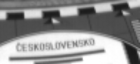
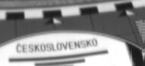
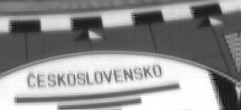
By neglecting the effect of the camera point spread function, the image formation matrix, $A^{(i)}$, can be approximated as the outcome of the geometric warp and down-sampling,

$$A^{(i)}=T^{(i)}.$$

Imagine that $T^{(i)}$ is implemented as bilinear interpolation, then this simplification introduces the obvious flaw that only 4 high-resolution pixels are used to calculate the value of any single low-resolution pixel. In reality, a low-resolution pixel may (and probably will) depend on more high-resolution pixels; the exact number being determined by the resolution increase, $z$, and the severity of the transformation, $H$. If the zoom ratio is chosen conservatively, the approximation may be sufficient, as illustrated in Figure 1.

Next, we examine the construction of such a bilinear interpolation operator. An improved polygon-based interpolation operator is then proposed to address its deficiencies.

5.1 Bilinear interpolation

The bilinear transformation/interpolation operator, $A=T$, has coefficients appearing on and around the diagonal. The coefficients in (6) are derived from bilinear interpolation as follows:

Suppose a function is known at four grid coordinates surrounding $(x,y)$, namely $f_{00}=f(\left\lfloor x\right\rfloor,\left\lfloor y\right\rfloor)$, $f_{01}=f(\left\lfloor x\right\rfloor,\left\lfloor y\right\rfloor+1)$, $f_{10}=f(\left\lfloor x\right\rfloor+1,\left\lfloor y\right\rfloor)$, and $f_{11}=f(\left\lfloor x\right\rfloor+1,\left\lfloor y\right\rfloor+1)$. The value at $f(x,y)$ is not available, but a two-fold linear interpolation approximates it as

$$f(x,y)\approx\left[\begin{array}[]{cc}1-u&u\end{array}\right]\left[\begin{array}[]{cc}f_{00}&f_{01}\\ f_{10}&f_{11}\end{array}\right]\left[\begin{array}[]{c}1-t\\ t\end{array}\right]\\ =f_{00}(1-u)(1-t)+f_{01}(t)(1-u)+f_{10}(u)(1-t)+f_{11}(u)(t)$$ (7)

with $u=x-\left\lfloor x\right\rfloor$ and $t=y-\left\lfloor y\right\rfloor$. This is known as bilinear interpolation (even though the successive combination of two linear operators is no longer linear). If all known grid-values of $f(x,y)$ are placed in a vector, $\mathbf{x}$, then

$$f(x,y)\approx\mathbf{a}^{T}\mathbf{x},$$ (8)

where $\mathbf{a}$ is a sparse vector of interpolation coefficients given by (7) ($\mathbf{a}$ has mostly zero entries, except where elements in $\mathbf{x}$ correspond to $f_{00},$ $f_{01}$, $f_{10}$, or $f_{11}$). When interpolating for several coordinate pairs $(x_{i},y_{i})$ simultaneously, (8) becomes

$$\mathbf{b}=A\mathbf{x},\quad\mathrm{with}\,\mathbf{b}=\left[\begin{array}[]{c}f(x_{0},y_{0})\\ f(x_{1},y_{1})\\ \vdots\\ f(x_{N-1},y_{N-1})\end{array}\right].$$ (9)

(a) With bilinear interpolation, the centre of the transformed pixel (big dot) is used to find the nearest surrounding pixel centres (small dots). Only those high-resolution pixels are used to compute the value of the low-resolution pixel, weighted according to their distance from the center of the transformed pixel.

(b) With polygon-based interpolation, all high-resolution pixels touching the transformed pixel are used in computing the value of the low-resolution pixel, according to the amount of overlap with the transformed pixel.

Figure 2: A comparison between the footprints of bilinear and polygon-based interpolation. Each figure shows a low-resolution pixel, transformed onto the high-resolution image.

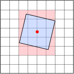
For super-resolution reconstruction, we need $A^{(i)}$ to warp and down-scale the high-resolution image, $\mathbf{x}$, to produce a given low-resolution image, $\mathbf{b}^{(i)}$. Recall that, after registration, the homeography $H_{i,0}$ that warps low-resolution image $i$ onto low-resolution reference image ($i=0$) is known. The homography that warps the high-resolution image to the $i$-th low-resolution image then becomes

$$M_{i}=\left(H_{i,0}\right)^{-1}S\quad\mbox{with}\quad S=\left[\begin{array}[]{ccc}1/z&0&0\\ 0&1/z&0\\ 0&0&1\end{array}\right].$$

Rewriting (9) as

$$\mathbf{b}^{(i)}=A^{(i)}\mathbf{x},\quad\mathbf{b}^{(i)}=\left[\begin{array}[]{c}f(M_{i}^{-1}\mathbf{c}_{0})\\ f(M_{i}^{-1}\mathbf{c}_{1})\\ \vdots\\ f(M_{i}^{-1}\mathbf{c}_{N-1})\end{array}\right]$$

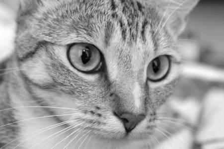
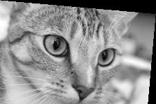
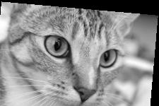
where $\mathbf{c}_{j}$, $j=0,\ldots,N-1$ represents all coordinates in a low-resolution frame. With the coordinates $M_{i}^{-1}\mathbf{c}_{j}$ known, the matrix $A^{(i)}$ can be constructed. Figure 4b illustrates the effect of $A$ on $\mathbf{x}$.

(a) Sparsity structure of the bilinear interpolation operator $A$. Note that no row contains more than 4 non-zero values.

(b) Sparsity structure of the polygon interpolation operator $A$. The first rows are empty, since the corresponding pixels fall outside of the input image. The rows contain more coefficients than in the case of the bilinear operator, indicating a larger footprint.

Figure 3: Comparison of the structures of the bilinear and polygon image formation matrices. In both cases, $A$ was constructed to rotate by $5^{\circ}$ and to downsample by 2. Only the first few rows of each operator is shown.

(a) High-resolution input image. The vector representation, $\mathbf{x}$, is obtained by unpacking the values in lexicographic order.

(b) The matrix-vector product, $A\mathbf{x}$, for the bilinear operator, reshaped to form an image.

(c) The matrix-vector product, $A\mathbf{x}$, for the polygon interpolation operator.

Figure 4: The effect of interpolation operators.

5.2 Polygon-based interpolation

In [16], a polygon intersection scheme, subsequently found to be similar to NASA’s Drizzle [6], is presented for image fusion. Both methods rely on intersecting quadrilaterals (four-cornered polygons that represent pixels) to determine pixel weights, but the formulation as a linear operator—as discussed in this paper—proves to be fundamental in its application to super-resolution imaging.

As in the previous section, we want to express a low-resolution output image as $\mathbf{b}=A\mathbf{x}$. Each pixel value, $b_{m}$, depends on a number of pixels from the high-resolution image, $\mathbf{x}$, weighted by the coefficients in row $m$ of the operator $A$. The motivation behind the polygon interpolation operator is as follows:

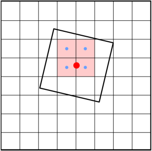
A camera sensor is a grid of photo-sensitive cells (think of them as photon buckets, each representing a pixel [9]). Due to micro-lenses, the gaps between cells are negligible. During imaging, the sensor irradiance is integrated over each cell for the duration of exposure, after which the values are read out as a matrix. Now, imagine two sensors, one with large cells (low-resolution) and the other with small cells (high-resolution), rotated relative to one another. How are the cell values for the different sensors related? Our proposed solution is to measure the overlap between the larger and smaller cells, as shown in Figure 2b. The value of a (large) low-resolution cell is set to a weighted sum of all (small) high-resolution cells, where the weights depend on their overlap.

For each low-resolution pixel, $b_{m}$:

1. Create a quadrilateral (four-node polygon) from the corner-points of $b_{m}$. For example, the pixel at $(0,0)$ would correspond to the polygon with nodes

   $$\mathbf{x}_{L}^{m} = (-0.5,0.5,0.5,-0.5)$$

   $$\mathbf{y}_{L}^{m} = (-0.5,-0.5,0.5,0.5).$$

   The subscript $L$ indicates “low-resolution” and the super-script is the pixel number.

2. Transform the polygon to the high-resolution frame, using the transformation matrix $M^{-1}$ given in the previous section. The new corner coordinates are $\mathbf{\hat{x}}_{L}^{m}$, $\hat{\mathbf{y}}_{L}^{m}$. If any of the coordinates fall outside the high-resolution image, break this loop and continue to the next low resolution pixel (there may be other ways to handle boundary problems, but this is simple and works well).

3. Determine the bounding box of the newly formed polygon:

   $$\mathbf{x}_{BB} = \left(\left\lfloor\mbox{$\min$}\mathbf{x}^{\prime}_{L}\right\rfloor,\left\lceil\mbox{$\max$}\mathbf{x}^{\prime}_{L}\right\rceil,\left\lceil\mbox{$\max$}\mathbf{x}^{\prime}_{L}\right\rceil,\left\lfloor\mbox{$\min$}\mathbf{x}^{\prime}_{L}\right\rfloor\right)$$

   $$\mathbf{y}_{BB} = \left(\left\lfloor\mbox{$\min$}\mathbf{y}^{\prime}_{L}\right\rfloor,\left\lfloor\mbox{$\min$}\mathbf{y}^{\prime}_{L}\right\rfloor,\left\lceil\mbox{$\max$}\mathbf{y}^{\prime}_{L}\right\rceil,\left\lceil\mbox{$\max$}\mathbf{y}^{\prime}_{L}\right\rceil\right)$$

4. For each high-resolution pixel inside the bounding box:

   1. Assign the pixel number $n=iN+j$ where $(i,j)$ is the grid position of the high-resolution pixel and $N$ is the total number of columns in the high-resolution frame.

   2. Create a quadrilateral from the corner-points of the high-resolution pixel with vertices $\mathbf{x}_{H}^{n}$ and $\mathbf{y}_{H}^{n}$.

   3. Measure the area of overlap between the polygons $(\mathbf{x}_{L}^{m},\mathbf{y}_{L}^{m})$ and $(\mathbf{x}_{H}^{n},\mathbf{y}_{H}^{n})$, and assign the value to $A_{m,n}$.

5. Divide each row $A_{m,*}$ by its sum so that the weights add to one.

Algorithm 1 Calculating the coefficients of the polygon interpolation operator $A$. Also see Figure 2b.

Algorithm 1 outlines the calculation of the coefficients in $A$. The operator is parameter free, and has a variable size footprint that covers all relevant high-resolution pixels (see Figure 3). Furthermore, it has less of a smoothing effect than the bilinear interpolator.

Computing the coefficients of $A$ is more expensive for polygon interpolation than for bilinear interpolation, due to the many polygon area intersection calculations (called “clipping” operations) involved. However, two conditions improve execution time when clipping: polygons from the high-resolution image are always aligned with the grid (horizontal and vertical boundaries), and all polygons involved are convex.

The first observation is particularly important, since it allows the use of algorithms that clip polygons to a “viewport” (typically used to determine which part of a polygon falls inside the screen). The second means that a simpler class of algorithm can be employed. We use the Liang-Barsky algorithm [12], which is specifically optimized for rapidly clipping convex polygons against a viewport. Another applicable approach is that by Maillot [13].

The area of the resulting non-self-intersecting clipped polygon is easily determined as given by [1]:

$$a=\frac{1}{2}\sum_{i=0}^{N-1}(x_{i}y_{i+1}-x_{i+1}y_{i}),$$

where $\mathbf{x}$ and $\mathbf{y}$ are the polygon vertices in either clock-wise or anti-clock-wise order. The clipping of the entire collection of pixels can easily be parallellized. Also, if only the result of the operator, $A\mathbf{x}$, is required, it can be rapidly rendered via a Graphical Processing Unit without explicitly calculating any polygon intersections manually (pixels are simply drawn as polygons and transformed; the GPU takes care of clipping in its fixed pipeline). Figure 4b illustrates the effect of $A$ on a vector $\mathbf{x}$.

Note that this interpolation model is only applicable before Bayer demosaicking (a process which destroys much of the super-resolution information in any case).

(a) Example input frame (one of thirty), upscaled by a factor of 4 using sinc (Lanczos) interpolation.

(b) All input frames, upsampled and averaged (stacked), after photometric registration.

(c) Super-resolution result after photometric registration, using polygon interpolation, zoom factor $z=4$, and $\lambda=0.05$. Note the appearance of the slanted brick-face.

Figure 5: Super-resolution result achieved with polygon-based interpolation.

6 Results and conclusion

As test data, we use 30 images and their corresponding homographic transformations to a chosen reference, obtained from a hand-held video of a library wall (see acknowledgements). We solve the regularized least-squares system in (4) using conjugate gradients (L-BFGS [19] and LSQR [15, 14] give comparable results). The prior $\mathbf{x}_{0}$ is chosen as the average of all low-resolution images, up-scaled. The high-resolution estimate $\mathbf{x}$ is then obtained from (5).

The results shown in Figures 1 and 5 prove the viability of the proposed method. Software that implements the entire super-resolution reconstruction is provided under an open source license at http://mentat.za.net/supreme.

We’ve shown that, in the context of super-resolution imaging, an interpolation operator based on polygon intersection holds several advantages: it models the underlying sensor physics, it is easy to compute, has a variable footprint that automatically adjusts to the underlying transformation and can easily be expressed as a linear operator. The method can also be extended to model pixels as higher order polygons, thereby allowing for non-linear image transformations between input images (such as those introduced by lens distortions).

More detail on the various aspects of super-resolution imaging presented here is given in [17].

Acknowledgements

The library data sequence is by Barbara Levienaise-Obadia, University of Surrey. Tomas Pajdla and Daniel Martinec, CMP, Prague provided the “text” dataset. Both were collected by David Capel and is available for download from http://www.robots.ox.ac.uk/~vgg/data.

References

?refname?
- [1] Paul Bourke. Calculating The Area And Centroid Of A Polygon. http://local.wasp.uwa.edu.au/~pbourke/geometry/polyarea/.
- [2] David Peter Capel. Image Mosaicing and Super-resolution. Ph.D. dissertation, University of Oxford, 2001.
- [3] P. Cheeseman, B. Kanefsky, R. Kraft, J. Stutz, and R. Hanson. Super-resolved surface reconstruction from multiple images. In G. R. Heidbreder, editor, Proceedings of the Thirteenth International Workshop on Maximum Entropy and Bayesian Methods. Kluwer Academic, 1993.
- [4] Hilda Faraji and W. James MacLean. CCD noise removal in digital images. IEEE Transactions on Image Processing, 15(9):2676–85, September 2006.
- [5] J. Fridrich. Digital Image Forensics. IEEE Signal Processing Magazine, 26(2):26–37, 2009.
- [6] A. S. Fruchter and R. N. Hook. Drizzle: A Method for the Linear Reconstruction of Undersampled Images. Publications of the Astronomical Society of the Pacific, 114(792):144–152, February 2002.
- [7] A. Garzelli, F. Nencini, L. Alparone, B. Aiazzi, and S. Baronti. Pan-sharpening of multispectral images: a critical review and comparison. IEEE International Geoscience and Remote Sensing Symposium, 2004. IGARSS ’04. Proceedings. 2004, pages 81–84.
- [8] F. Guichard and L. Rudin. Velocity estimation from images sequence and application to super-resolution. In Proceedings of the 1999 International Conference on Image Processing, pages 527–531. IEEE, 1999.
- [9] G.E. Healey and R. Kondepudy. Radiometric CCD camera calibration and noise estimation. IEEE Transactions on Pattern Analysis and Machine Intelligence, 16(3):267–276, 1994.
- [10] James R. Janesick. Scientific charge-coupled devices. SPIE Press, 2001.
- [11] Anat Levin, Yair Weiss, and Dani Lischinski. Colorization using optimization. ACM Transactions on Graphics, 23(3):689, 2004.
- [12] You-Dong Liang and Brian A. Barsky. An analysis and algorithm for polygon clipping. Communications of the ACM, 26(11):868–877, 1983.
- [13] Patrick-Gilles Maillot. A new, fast method for 2D polygon clipping: analysis and software implementation. ACM Transactions on Graphics, 11(3):276–290, July 1992.
- [14] Christopher C. Paige and Michael A. Saunders. Algorithm 583: LSQR: Sparse Linear Equations and Least Squares Problems. ACM Transactions on Mathematical Software, 8(2):195–209, June 1982.
- [15] Christopher C. Paige and Michael a. Saunders. LSQR: An Algorithm for Sparse Linear Equations and Sparse Least Squares. ACM Transactions on Mathematical Software, 8(1):43–71, March 1982.
- [16] S. J. van der Walt and B. M. Herbst. Methods used in increased resolution processing: polygon-based interpolation and robust log-polar based registration. In Proceedings of the International Conference on Computer Vision Theory and Applications (VISAPP) 2007, Barcelona, Spain, 2007.
- [17] Stéfan van der Walt. Super-resolution Imaging. PhD thesis, Stellenbosch University, 2010.
- [18] John Wright and Thomas Huang. Image super-resolution as sparse representation of raw image patches. 2008 IEEE Conference on Computer Vision and Pattern Recognition, June 2008.
- [19] Ciyou Zhu, Richard H. Byrd, Peihuang Lu, and Jorge Nocedal. Algorithm 778: L-BFGS-B: Fortran subroutines for large-scale bound-constrained optimization. ACM Transactions on Mathematical Software (TOMS), 23(4), 1997.