Statistical mechanics of graph models
and their implications for emergent manifolds

Abstract

Inspired by “quantum graphity” models for spacetime, a statistical model of graphs is proposed to explore possible realizations of emergent manifolds. Graphs with given numbers of vertices and edges are considered, governed by a very general Hamiltonian that merely favors graphs with near-constant valency and local rotational symmetry. The ratio of vertices to edges controls the dimensionality of the emergent manifold. The model is simulated numerically in the canonical ensemble for a given vertex to edge ratio, where it is found that the low-energy states are almost triangulations of two-dimensional manifolds. The resulting manifold shows topological “handles” and surface intersections in a higher embedding space, as well as non-trivial fractal dimension consistent with previous spectral analysis, and nonlocal links consistent with models of disordered locality. The transition to an emergent manifold is first order, and thus dependent on microscopic structure. Issues involved in interpreting nearly-fixed valency graphs as Feynman diagrams dual to a triangulated manifold as in matrix models are discussed. Another interesting phenomenon is that the entropy of the graphs are super-extensive, a fact known since Erdős, which results in a transition temperature of zero in the limit of infinite system size: infinite manifolds are always disordered. Aside from a finite universe or diverging coupling constraints as possible solutions to this problem, long-range interactions between vertex defects also resolve the problem and restore a nonzero transition temperature, in a manner similar to that in low-dimensional condensed-matter systems.

I Introduction

Since the first systematic studies of random graph models by Erdős and Rényi Erdős and Rényi (1959), the relation between graph theory models and physics models, in particular statistical physics models, has attracted much interest. Concepts and tools in graph theory have been applied to problems in physics, computer science, and biology to produce remarkable results. For example, Feynman diagrams that are planar have special roles in the large $N$ QCD model ’t Hooft (1974); in causal dynamical triangulation, four-dimensional triangulated manifolds with fixed edge lengths, which can be viewed as a class of graphs, are used to construct spacetime on the Planck scale to regularize the quantum gravitational path integral Ambjørn et al. (2004, 2005a); statistical mechanical models of network growth can explain the connectivity of systems such as the Internet Albert and Barabási (2002); structures of amorphous solids can be quantified using graph theory properties Franzblau (1991); intracellular signalling networks can exhibit emergent behavior stored within biochemical reactions, including integration of signals across multiple time scales and self-sustaining feedback loops Bhalla and Iyengar (1999); neural networks can collectively and robustly produce content-addressable memories from partial cues Hopfield (1982), indicating capacity for generalization, familiarity recognition, and categorization. Added to these discoveries, a new collection of graph models has been proposed as candidates for emergent spacetime, as described below.

A manifold can be approximated by a triangulation, which in turn can be viewed as a graph filled with simplices. From this observation, one can consider how a graph may give rise to a manifold; i.e. from a family of graphs, following some constraints and obeying some set of rules for dynamical processes, is it possible that a manifold-like structure can emerge? To be more precise, consider the possibility that a graph $G$ gives rise to a smooth manifold $M$. A vertex in $G$ corresponds to a point in $M$; when a pair of vertices in $G$ are connected by an edge, the corresponding pair of points in $M$ have a certain distance $\epsilon$. When the length scale under consideration is much larger than $\epsilon$, $G$ resembles the smooth manifold $M$. In such cases, one can say that the manifold $M$, including its dimensionality, topology, and metric, emerges from the graph $G$ in the continuous limit.

From this general idea, in references Konopka et al. (2006, 2008), a graph model was constructed from a given graph Hamiltonian, where it was proposed that the low-energy phase of the model may be interpreted as an emergent spacetime. In addition, it was found that when the edges of the graph possess a spin degree of freedom, the model could give rise to a U(1) gauge theory Konopka et al. (2008). In Konopka (2008), Konopka has analytically and numerically studied the above graph model as a statistical model. A phase transition was found, where it was argued that the low-temperature phase can be related to spacetime only if the graph can interact with some matter degrees of freedom. In Hamma et al. (2010); Caravelli et al. (2012), a related model, which in addition to graphs corresponding to spacetimes, also incorporates a matter field that resides on the vertices, was proposed to study the role of matter in the emergence of spacetime from graphs. In Conrady (2011), Conrady has constructed a Hamiltonian favoring low-temperature, two-dimensional manifolds through terms that explicitly favor two-dimensional triangulations; for example, each vertex is favored to have 6 edges as in a triangular lattice, and tetrahedra are penalized. The model was simulated for small system sizes ($N\leq 180$ edges), which showed a heat capacity peak, and a transition temperature that decreased with system size.

In this paper, we also investigate a statistical model of graphs, in that the objects under consideration are merely abstract graphs, without any information on the positions of the vertices, or the lengths of the edges. A graph can randomly transform into another graph according to a set of transformation rules. Graphs with given numbers of vertices and edges are considered, and they are governed by a Hamiltonian that favors graphs with a set of local symmetries. If these local symmetries are preserved, the resulting graphs should be nearly triangulations of manifolds with a certain dimensionality, where the dimensionality is controlled by the ratio of vertices to edges. We are interested in whether any global structure of the graphs arises as a consequence.

Because every edge in this model corresponds to a positive length $\epsilon$, only real positive distances can arise, so this model can only be used to describe Riemannian manifolds (i.e., with positive definite metric). The metric of a Riemannian manifold can be alternatively viewed as a distance function between any pair of points, which satisfies the triangle inequality. On a graph, there is also a natural notion of distance, namely the length of the shortest path between a pair of vertices. This distance is also positive-definite and satisfies the triangle inequality. Thus on any graph, there is a well-defined distance function, as well as a corresponding geodesic. Graph geodesics between two vertices are often highly degenerate, however, unlike the case for manifolds. If a manifold is to emerge from a graph, one expects that in the continuous limit all degenerate geodesics are close by, and the differences of their paths are only of order $\epsilon$. After establishing this distance function between vertices, mapping the graph to a Riemannian manifold is still a non-trivial problem. If we enforce that every edge is identical in that they have the same length when mapped to the Riemannian manifold, then only for certain graph configurations will a Riemannian manifold emerge from the graph. Otherwise the system will be frustrated and unable to meet the condition of constant edge length, without increasing the dimension above that of the manifold that would emerge from the graph.

In this paper, after reviewing the relevant graph theory preliminaries, we introduce a graph Hamiltonian based only upon local symmetries. We evolve the graph under the Monte Carlo rules obeying statistical mechanical equilibrium, and we investigate whether a low-temperature manifold state emerges. We investigate the sharpness of the phase transition using energy as an order parameter for different size systems, and we discuss the likely first-order nature of the transition. We construct heat capacity curves as a function of temperature and investigate the transition temperature as a function of system size, which points toward a zero-temperature phase transition in the bulk limit. The Haussdorf dimensionality of the emergent manifold is investigated and found to be an increasing function of system size, and approximately 3 for the largest system sizes we investigated (2000 vertices). Correlation functions between defect-carrying vertices and edges are investigated to determine whether the effective potential between defects is attractive or repulsive. Finally, we argue in analogy to condensed-matter systems that a nonzero phase transition temperature requires long-range interactions, and show that a Coulombic-like term between graph vertices yields an apparently finite-phase transition temperature, but with a highly ramified manifold.

II Graph theory preliminaries

Figure 1: Examples for the graph theory concepts.

Before motivating for details of the model, we shall remind the reader about some graph theory concepts, which will be needed later in constructing the model.

A graph $G$ is composed of a set of vertices $V(G)$ and a set of edges $E(G)$, where every edge is a subset of $V(G)$ with two elements. Note that by this definition, the two vertices in an edge set cannot be the same vertex, and two edges cannot connect the same two vertices. Such graphs are sometimes called “simple graphs,” as opposed to “multigraphs.” Because we will only consider graphs of this definition, they will be simply referred to as “graphs.”

A vertex $v$ is incident with an edge $e$ if $v\in e$. We denote an edge $e$ by its vertices, or ends, say $u$ and $v$, as $e=\{u,v\}$, or simply $e=uv$. A vertex $u$ is a neighbor of, or is adjacent to, a vertex $v$ if $uv$ is an edge. The valency or degree of a vertex is the number of edges incident to that vertex.

A graph in which every vertex has the same valency is regular. It is $k$-regular if every vertex has valency $k$.

A graph in which every pair of vertices is connected by an edge is complete. It is denoted by $K_{n}$ if it has $n$ vertices.

$G^{\prime}$ is a subgraph of a graph $G$, if $G^{\prime}$ is a graph, $V(G^{\prime})\subseteq V(G)$ and $E(G^{\prime})\subseteq E(G)$, and this is denoted by $G^{\prime}\subseteq G$.

If $U\subseteq V(G)$, the subgraph $G^{\prime}$ induced by $U$ is the graph for which $V(G^{\prime})=U$, and $E(G^{\prime})$ contains an edge $xy$ if and only if $x,y\in U$ and $xy\in E(G)$. This is denoted by $G^{\prime}=G[U]$, and $G^{\prime}$ is called an induced subgraph of $G$. (For example, in Fig. 1, the vertices $k,o,p,s$, and the five thick edges, compose an induced subgraph; the vertices $i,m,n,q$, and the four thick dotted edges, compose a subgraph, but not an induced subgraph.) In particular, in a graph $G$, the subgraph induced by the set of neighbors of a vertex $v$ is called the neighborhood of $v$, and is denoted by $G_{N}(v)$.

A path is an alternating sequence of vertices and edges, beginning with a vertex and ending with a vertex, where each vertex is incident to both the edge that precedes it and the edge that follows it in the sequence, and where the vertices that precede and follow an edge are the end vertices of that edge. The length of a path is the number of edges in the path. (For example, in Fig. 1, $(a,ab,b,bf,f,fg,g)$ is a path with length 3, in which the edges are denoted by dotted lines, and is also one of several paths between $a$ and $g$ having the minimal distance.) The distance between two vertices is the length of shortest path between them. In a graph $G$, the distance between vertices $u,v$ is denoted by $d_{G}(u,v)$.

A graph is connected if any two vertices are linked by a path.

The eccentricity $\epsilon_{G}(v)$ of a vertex $v$ in a graph $G$ is the maximum distance from $v$ to any other vertex, i.e.,

$$\epsilon_{G}(v)=\max_{u\in V(G)}d_{G}(v,u),$$

where $d_{G}(v,u)$ is the distance between $v$ and $u$ in the graph $G$.

The diameter $\textrm{diam}(G)$ of a graph $G$ is the maximum eccentricity over all vertices in a graph, and the radius $\textrm{rad}(G)$ is the minimum,

$$\textrm{diam}(G)=\max_{v\in V(G)}\epsilon_{G}(v),\quad\textrm{rad}(G)=\min_{v\in V(G)}\epsilon_{G}(v).$$

When $G$ is not connected, $\textrm{diam}(G)$ and $\textrm{rad}(G)$ are defined to be infinite. Some examples of neighborhood subgraphs are shown in Fig. 2. For every vertex in Fig. 1, the neighborhood subgraph is Fig. 2(a); for every vertex in Fig. 3, the neighborhood subgraph is Fig. 2(f). Figures 2(b)-2(e) are examples of neighborhood subgraphs that appear commonly in the simulation.

Figure 2: Some examples of neighborhood subgraphs. The eccentricity is labeled for each vertex, and the difference of diameter and radius of these subgraphs, which is denoted by $\Delta$, is labeled below each graph. (a) is the neighborhood subgraph of vertices in the triangular lattice graph (Fig. 1); (b), (c), (d) and (e) appear commonly in simulations, as parts of the defects; (f) is the neighborhood subgraph of vertices in the graph in Fig. 3.

Given a lattice, the corresponding lattice graph is the graph whose vertices are the points in the lattice, and whose edges are the pairs of nearest points in the lattice. (For example, the whole graph in Fig. 1 is an equilateral triangular lattice graph.)

III The model

To gain intuition on the form of constraints and Hamiltonians that may induce manifolds, let us construct some graphs resembling some manifolds, starting with the example of a flat two-dimensional plane $\mathbb{R}^{2}$. Intuitively, any two-dimensional lattice graph as defined above forms a “two-dimensional” manifold, and a coordinate system of the manifold naturally inherits from the coordinates of the lattice graph. This is directly analogous to a Bravais lattice in crystallography. A priori there seems no decisive reason to choose any particular Bravais lattice as the preferred graph configuration; however, we shall choose the equilateral triangular lattice graph (Fig. 1), using the following argument. On $\mathbb{R}^{2}$, for any point $p$ and any distance $\delta$, let $B_{\delta}(p)$ denote the geodesic ball centered at $p$ with radius $\delta$, and $B_{\delta}(p)-p$ has the topology of a circle $S^{1}$. For graphs, we can define the notion of “geodesic ball” similarly with that in Riemannian geometry. Let $B_{n}(v)$ be the set of the vertices that have distance from vertex $v$ no greater than $n$, including $v$ itself. For any two-dimensional lattice, if we denote the corresponding graph by $G$, for sufficiently large $n$, the induced subgraph $G[B_{n}(v)-v]$ also looks like $S^{1}$ topologically. However, for $n=1$, namely the neighborhood subgraph $G_{N}(v)=G[B_{1}(v)-v]$, this property is no longer true for all lattices. For example, on the square lattice, $G_{N}(v)$ is composed of 4 disconnected vertices. Only for the equilateral triangular lattice, $G_{N}(v)$ looks topologically like $S^{1}$. Thus in this sense, the equilateral triangular lattice graph is the closest analog to $\mathbb{R}^{2}$ among all the two-dimensional lattice graphs, on all distance scales down to $\epsilon$.

A graph can form a two-dimensional lattice for the correct ratio of edges to vertices. While a thermalized lattice in two dimensions is isotropic Mermin and Wagner (1966); Hohenberg (1967); Coleman (1973), the connectivity of such a lattice is still well-defined at low temperature. We thus choose to add defects in the form of extra edges or bonds, which will evolve under some Hamiltonian. This allows bonded vertices to be permuted, so that the low-temperature phase is still a “quasi-fluid” that retains a symmetry corresponding to randomized graph connectivities. The extra edges induce defects in the lattice, which may be mobile. The exact shape of the defects and the reason why the defects are unstable or meta-stable depend sensitively on the Hamiltonian. We shall construct a candidate Hamiltonian, and test the stability of the defects by numerical simulation. This construction generalizes to $\mathbb{R}^{n}$ straightforwardly: We can see that the defect-free lattice is the $n$-dimensional lattice as arising from a regular tiling of $n$-dimensional tetrahedra. The defect is a $(n-1)$-dimensional “foam” that divides the space into many patches of lattices with random orientations.

We seek the simplest Hamiltonian that can give rise to manifold-like triangulation graphs as classical solutions, which contain defects that facilitate graph permutation symmetry. We assume that the action is local, in the sense that it should be a sum over the vertices and/or edges, such that each term involves a finite number of vertices and/or edges within some cutoff distance. This condition is imposed because almost all physics models for which the Hamiltonian or Lagrangian is an integral of the corresponding density are local in the same sense.

A defect manifests itself as a local structure containing vertices with anomalous valency. One obvious local property of manifold-like graphs is that all vertices not in any defects would have the same valency. Moreover it is likely that vertices in the defects have just one more or one less neighbor. These properties can be enforced by a Hamiltonian quadratic in the valency:

$$H_{1}=c_{1}\sum_{v\in V(G)}n_{v}^{2},$$ (1)

where $n_{v}$ is the valency of vertex $v$, and $c_{1}$ is a positive constant (which will be taken to be infinite as described below). The average valency of the vertices is given by

$$\alpha=\frac{2N_{E}}{N_{V}}$$ (2)

where $N_{E}$ is the total number of edges and $N_{V}$ the total number of vertices. Note that, for example, $\alpha=6$ is compatible with a regular equilateral triangular lattice, which in turn implies that the emergent manifold is two-dimensional, while $\alpha=12$ is compatible with the face-centered cubic lattice, which implies a three-dimensional emergent manifold. Thus without changing the form of the Hamiltonian, we should be able to find manifolds with different dimensionalities by adopting different a priori values of $\alpha$. In the simulations described below, we choose $\alpha$ to be a non-integer, so that there exists an “excess” number of edges, which contribute to the presence of defects. Because the total number of vertices and edges are fixed, the term in (1) is minimized when every vertex has valency either $\lfloor\alpha\rfloor$ or $\lceil\alpha\rceil$. In our simulations, $c_{1}$ is taken to be infinite and so is no longer an adjustable parameter of the model, and the corresponding term in (1) is enforced to be minimal.

To obtain manifold-like solutions consisting of patches of close-packed lattices interspersed with defects, it is not sufficient to impose only the condition that each vertex has approximately the same number of neighbors. Many regular graphs do not look like any manifold at all (see, for example, Fig. 3). Additional terms in the Hamiltonian are thus required for manifold-like solutions.

One candidate for such a term consists of particular subgraphs that can be embedded into the graph. From this viewpoint, $n_{v}$ is the number of $K_{2}$ subgraphs (two vertices connected by an edge) that go through the vertex $v$. It is likely however that choosing more terms of this type will affect the dimensionality of the resulting spacetime. For example, if we incorporate terms that favor more $K_{3}$ subgraphs (triangles) and fewer $K_{4}$ subgraphs (tetrahedra), then it can be expected that these terms would favor two-dimensional manifolds Conrady (2011). As we hope to find a model that does not select the dimensionality at the level of the Hamiltonian, we will not use any other term of this type besides $H_{1}$.

Figure 3: A 6-regular graph that is not similar to any manifold. This graph can be viewed as an infinite rooted “tree” graph, in which each node has three children (except the root node has four children), and every node of the “tree” is actually a tetrahedron.

Another property of manifold-like graphs is that around most vertices, the graph has a local discrete rotational symmetry that reflects the local isotropy of the emergent manifold. This can be restated as for each vertex $v$, the subgraphs $G[B_{n}(v)-v]$ for most $v$ should have a discrete rotational symmetry. To reduce the number of possible Hamiltonian terms, we impose this condition only on $G[B_{1}(v)-v]$, which is also $G_{N}(v)$. We introduce the term

$$H_{2}=c_{2}\sum_{v\in V(G)}\Delta(v),$$ (3)

where $c_{2}$ is a positive constant, and

$$\Delta(v)=\textrm{diam}(G_{N}(v))-\textrm{rad}(G_{N}(v)),$$ (4)

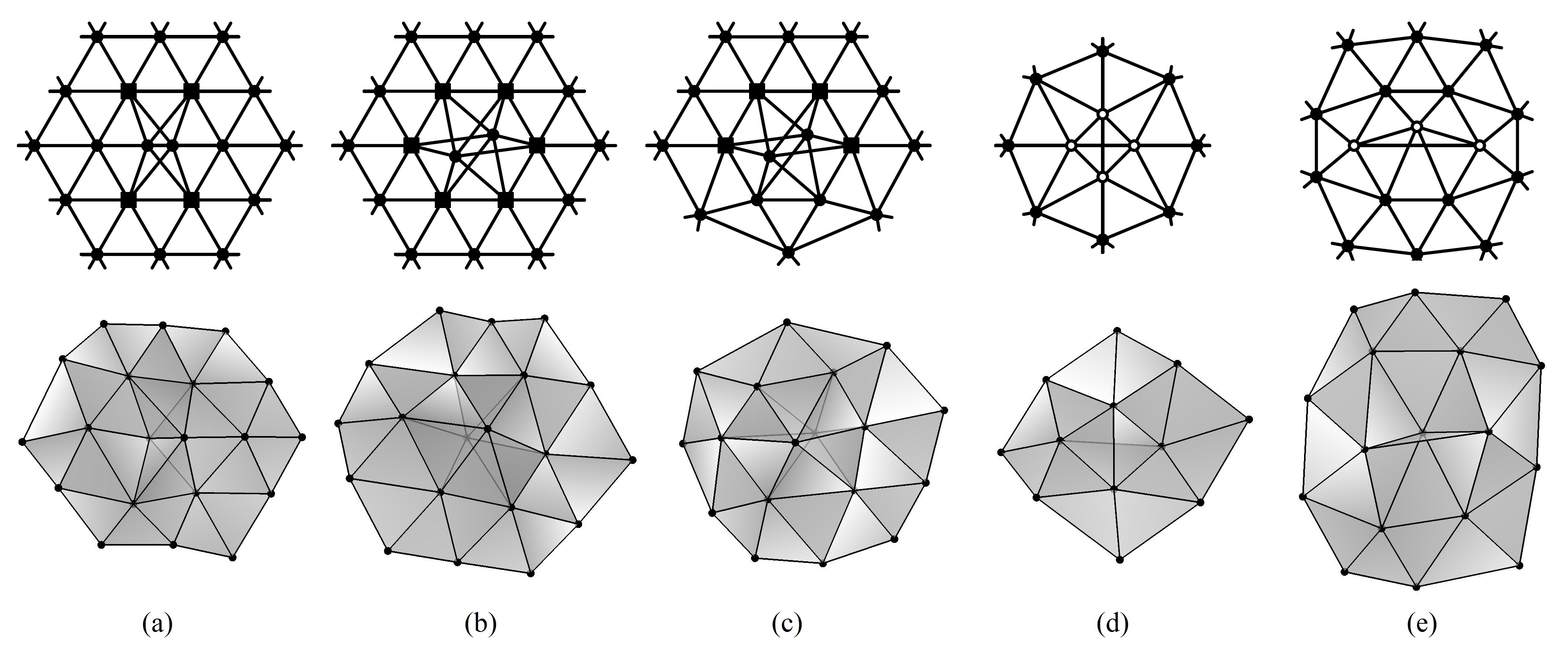
in which $\textrm{diam}(G_{N}(v))$ is the diameter of the subgraph $G_{N}(v)$, and $\textrm{rad}(G_{N}(v))$ is the radius of the subgraph $G_{N}(v)$. By the definitions of diameter and radius of graphs, if the subgraph $G_{N}(v)$ is not connected, they are both infinite. Here, we additionally define that their difference $\textrm{diam}(G_{N}(v))-\textrm{rad}(G_{N}(v))$ is also infinite when $G_{N}(v)$ is not connected. The term $H_{2}$ then enforces that all neighborhood subgraphs are always connected. When $G_{N}(v)$ is connected, the difference between its diameter and its radius is a measure of its asymmetry. Figure 2 shows several examples of neighborhood subgraphs. The eccentricity of every vertex in the subgraphs is labeled, along with the value of $\Delta(v)$ for each subgraph. For Figs. 2(a) and (b), the $G_{N}(v)$’s have a rotation symmetry of $\mathbb{D}_{6}$ and $\mathbb{D}_{7}$, respectively, while Figs. 2(c)-(e) are not rotationally symmetric.

In two dimensions, a graph forms a triangulation of a surface if and only if all the neighborhood subgraphs are cycles Malnič and Mohar (1992). When the degrees of the subgraphs are either 6 or 7, which is imposed by the $H_{1}$ term, one can see from the examples in Fig. 2 that the $H_{2}$ term indeed favors cyclic neighborhood subgraphs, with only one exception shown in Fig. 2(e). We thus expect that, in this model, a graph with low energy is almost a triangulation of a surface.

Thus we propose the following model: Consider a simple graph with $N_{V}$ vertices and $N_{E}$ edges. All the vertices are labeled, so isomorphic configurations with different labeling are considered to be different configurations. The Hamiltonian is composed of two terms, as motivated previously:

$$H=H_{1}+H_{2}.$$ (5)

Because the Hamiltonian is prohibitive to analytical solution, we implement a numerical simulation, as described in the next section, to study the equilibrium states of this model in the canonical ensemble, i.e. at a given temperature. In particular, we will be interested in the structures of the states with low energies, and the nature of the phase transition, if one exists, to these low-energy states.

IV Numerical simulation

We sample equilibrium states in the model using a Monte Carlo simulation Newman and Barkema (1999). The parameter $\alpha$ defined in (2) as giving the mean number of edges per vertex is taken to be slightly larger than 6, which we expect will induce two-dimensional structures dictated by triangulations as described above. There is no fixed boundary on the graphs. The size of the graphs is specified by the number of vertices $N_{V}$, and the number of edges $N_{E}$. For convenience, in the following we use $N_{V}$ and the number of extra edges $X\equiv N_{E}-3N_{V}$, to specify the size of the graphs. Given the graph size, the initial configuration is taken to be a randomly generated, connected graph.

The graph is evolved in the canonical ensemble with temperature $1/\beta$. In each Monte Carlo step, one end of an edge can jump from one vertex to another. We randomly pick an edge, and randomly label its ends by $u$ and $v$. To find the new location of the edge $uv$, we perform a random walk starting from $v$ as the origin, which does not pass through the edge $uv$ (this condition guarantees that a connected graph remains connected after such a move). The number of steps $\ell$ of the walk is a random positive integer chosen from the probability distribution $P(\ell)=\gamma^{\ell-1}-\gamma^{\ell}$, where $\gamma$ is a parameter between 0 and 1 (we take $\gamma=0.5$ below). Denote the ending vertex of the random walk as $v^{\prime}$. The edge is then moved from $uv$ to $uv^{\prime}$. If the new graph is still simple, its energy is compared with that of the old graph, and this move is accepted or rejected according to the Metropolis algorithm Newman and Barkema (1999). Each “sweep” through the system contains $N_{E}$ Monte Carlo steps, so on average each edge has one chance to jump in one sweep. Such a method is ergodic; moreover with this jumping scheme, the energy of only a few vertices is affected after each Monte Carlo step, and the energy of only these vertices needs to be updated.

Simulations are performed with $c_{1}=\infty$, $c_{2}=1.0$, $\gamma=0.5$, and various values of $N_{V}$, $X$ and $\beta$. Before showing the thermodynamics results from the simulations, let us first describe the method that we used to render a graph from the simulations, in order to interpret its evolution.

IV.1 Rendering graphs

To render a graph such that its structure can be best visualized, we need to devise an appropriate drawing scheme. A drawing of a graph maps vertices to points in $\mathbb{R}^{n}$ with line segments connecting adjacent points. The following method is used to generate drawings in $\mathbb{R}^{3}$. For any drawing of a graph $G$, we seek to minimize the function

$$H_{\textrm{draw}}=\sum_{e\in E(G)}\left(a_{1}l_{e}^{2}+\frac{a_{2}}{l_{e}^{2}}\right)+\sum_{\begin{subarray}{c}i,j\in V(G),\ i\neq j,\\ i,j\textrm{ not adjacent}\end{subarray}}\frac{a_{3}}{l_{ij}^{2}},$$ (6)

where $l_{e}$ is the length of the drawing of edge $e$, $l_{ij}$ is the distance of the drawing between vertices $i,j$, and $a_{1}=1.0,a_{2}=1.0,a_{3}=5.0$. The first term gives a preferred length for every edge, and the second term gives a repelling force to every non-adjacent pair of vertices. The function $H_{\textrm{draw}}$ is chosen this way in order to make every edge have approximately the same length in the drawing, and as well, to make the drawing as expanded as possible. In practice, even for moderate-sized graphs, $H_{\textrm{draw}}$ has numerous local minima and is difficult to minimize. We thus use another Monte Carlo calculation to search for its near-optimal values. Initially, all the vertices are located at the origin of $\mathbb{R}^{3}$. In each Monte Carlo step, a randomly-chosen vertex is randomly moved to another position within the ball of radius $\delta=2.5$, centered at the original position, and the new position has uniform probability distribution within the ball. After the Monte Carlo calculation, because the low-temperature configurations in the model are conjectured to be similar to triangulations of surfaces, we also search for all the $K_{3}$ subgraphs (triangles) in the graph, and render (flat, solid) triangles to fill the interior of the $K_{3}$’s.

Figure 4: (Color online) Some snapshots from the simulations, drawn in three dimensions. Panels (a)-(c) are for the system with number of vertices $N_{V}=200$ and number of extra edges $X=20$, where (a) is the initial configuration, (b) is a typical configuration at high temperature ($\beta=1.0$), and (c) is a typical configuration at low temperature ($\beta=2.0$). Compared with the sphere, the drawing (c) has three more handles, and the surface intersects with itself in three places, so it has a non-trivial, non-orientable topology. Panel (d) is for the system of size $N_{V}=1000$ and $X=100$, and shows a typical configuration at low temperature ($\beta=2.0$). In these drawings, if a vertex has valency 6, it is black if its $\Delta$ value is zero, and is red if its $\Delta$ value is nonzero; if a vertex has valency 7, it is green if its $\Delta$ value is zero, and is blue if its $\Delta$ value is nonzero (see text). As well, yellow lines are drawn at places where two triangles intersect, and the manifold thus passes through itself.

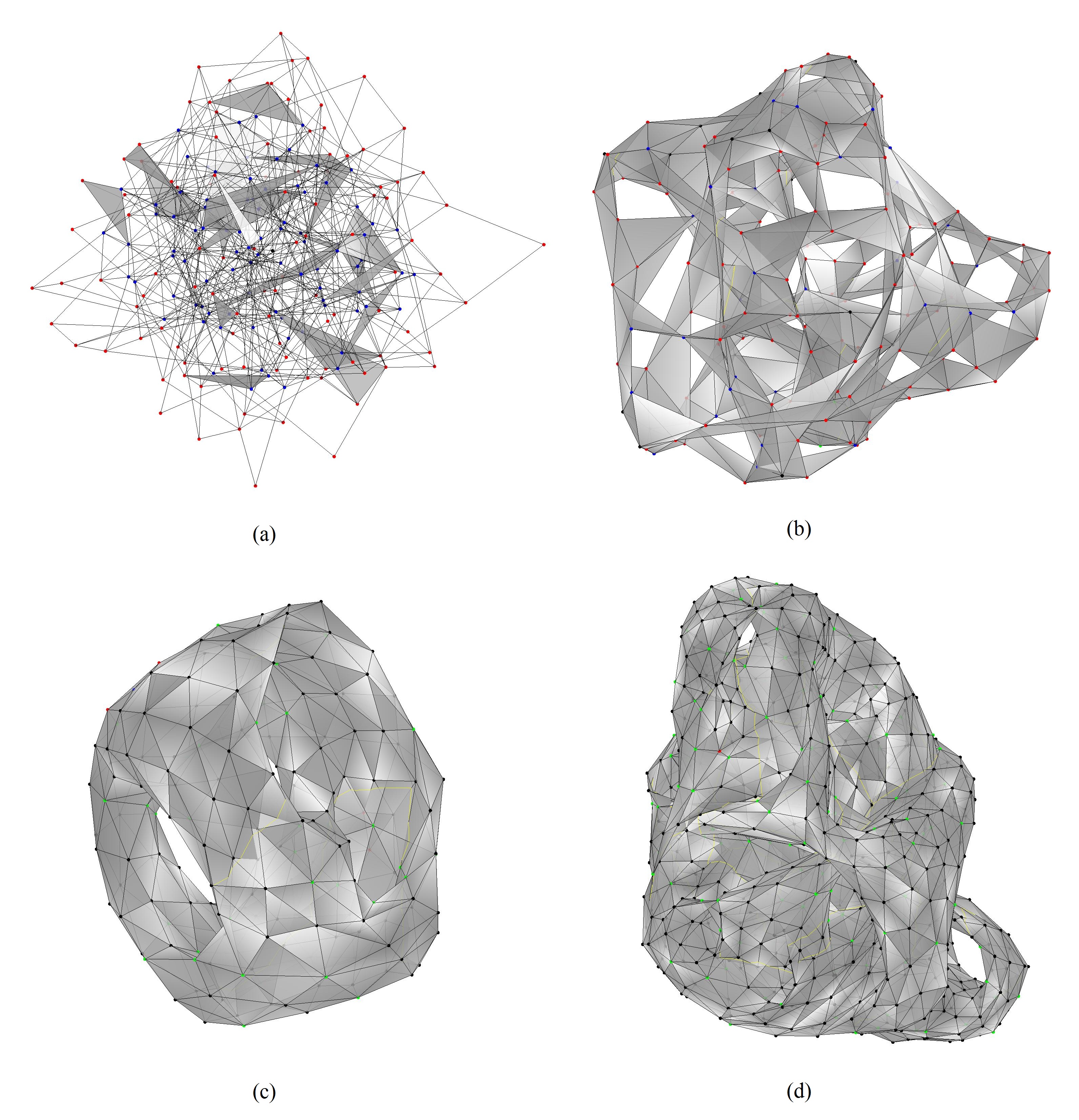
Figure 4 shows some snapshots taken from the simulations. Figures 4(a)-(c) are for the system of size $N_{V}=200$ and $X=20$. Figure 4(a) shows the initial configuration, 4(b) shows a typical configuration at high temperature ($\beta=1.0$), and 4(c) shows a typical configuration at low temperature ($\beta=2.0$). Figure 4(d) is for the system of size $N_{V}=1000$ and $X=100$, and it is a typical configuration at low temperature ($\beta=2.0$).

In the sample drawings in Fig. 4, different colors are used to denote different types of vertices. The color-code is as follows:

	Degree$=6$	Degree$=7$
Zero contribution to $H_{2}$	black	green
Nonzero contribution to $H_{2}$	red	blue

Also, yellow lines are drawn at places where two triangles intersect, i.e., this identifies where the triangulated surface intersects with itself.

Figure 5: Examples of some common defects. Once the graph is triangulated to construct a surface, defects (a-d) have “bubble-wrap” morphology, while defect (e) has “frenulum” morphology. The figures in the first row are the schematic drawing of the defects, in which a vertex is marked with a square if its valency is 7, a vertex is marked with an open circle if it contributes positive energy to $H_{2}$, and otherwise a vertex is marked with a filled circle. The figures in the second row are the corresponding drawings of the defects using the method described in subsection IV.1. Compared with the equilateral triangular lattice, examples (a), (b), (c), (d) and (e) have 2, 3, 2, 0, 0 extra edges, respectively.

IV.2 Topology of the manifold in the presence of defects

For the low-temperature graphs, several examples of common local defects are shown in Fig. 5. They are called local in the sense that in the vicinities of these defects, the graph is similar to some triangulation of surfaces with trivial topology. Among these examples, the “bubble-wrap” defects (a)-(c) do not increase the total energy, and around such defects the ratio between the number of edges and vertices is larger than 3. In other words, these defects can “absorb” the extra edges without energy cost. Also note that (a) and (b) do not change the long range order of the lattice orientation, while (c) does alter the long range order. Taken together, these defects induce configurational degeneracies in all the energy levels, including the ground state energy level, and at the same time induce graph permutation symmetry by randomly breaking the lattice’s long range order, at least in the rendering scheme of the manifold described above. The bubble wrap defect (d) and “frenulum” defect (e) increase the total energy, and alter the lattice orientation more drastically.

As discussed above, low-temperature graphs in the model are similar to two-dimensional triangulated surfaces. However, they contain local defects, and there are overall topological features of the surfaces that emerge from the graphs. For example, in the drawing Fig. 4(c), one can see that the emergent surface contains several handles, and the surface intersects itself in several places. In the drawing Fig. 4(d), the topology of the emergent surface is too intricate to easily identify. The Hamiltonian does not constrain the topology in any way, so in general, emergent surfaces of low-temperature graphs in the model have complicated topologies. The emergent surfaces have potentially many handles, and are in general non-orientable, in that there is no separation between interior and exterior sides of the surface. In our simulations, we also observe that the topology of the graphs’ emergent surfaces can dynamically change, even at a low energy.

We note, however, that the choice of $N_{V}$ and $N_{E}$ can constrain the topology. At low temperatures, the graphs are nearly triangulations, albeit with potentially complicated topologies. If a graph is strictly a triangulation, and we denote the number of triangles as $N_{F}$, then the Euler characteristic $\chi$ of the surface is given by $\chi=N_{V}-N_{E}+N_{F}$. For a triangulation, $3N_{F}=2N_{E}$; and we previously defined $N_{E}=3N_{V}+X$. Putting these three equations together, we find $\chi=-X/3$. As we showed above, defects on the graphs can absorb edges, so the relation for the nearly-triangulated graphs becomes an inequality $\chi\geq-X/3$. In addition, for any surface, $\chi\leq 2$, with $\chi=2$ corresponding to the topology of a sphere. Thus the Euler characteristic $\chi$ of the emergent surface can take any integer value between $-X/3$ and $2$. The $X$ values used in our simulations are not very small, so this constraint still allows for many possible different topologies for the emergent surface.

IV.3 Phase transition

In this sub-section we study the transition between the low-/high- temperature phases. For system sizes $N_{V}=100,200,300,500,1000,1500,2000$, and number of excess edges $X=0.1N_{V}$, the expectation value of energy $\langle E\rangle$, and the heat capacity $C=\beta^{2}\left(\langle E^{2}\rangle-\langle E\rangle^{2}\right)$ are computed for various inverse temperatures $\beta$, where the angle bracket here means averaging over all the samples in a simulation.

Figure 6: (Color online) The average energy density $\left\langle E\right\rangle/N_{V}$ as a function of inverse temperature $\beta$ for for several $N_{V}$’s indicated in the legend.

Figure 7: (Color online) The rescaled heat capacity $C/N_{V}^{2}=\beta^{2}\left(\left\langle E^{2}\right\rangle-\left\langle E\right\rangle^{2}\right)/N_{V}^{2}$ as a function of inverse temperature $\beta$ for several $N_{V}$’s indicated in the legend.

Figure 8: Log-log plot of the inverse transition temperature $\beta_{c}$ in the model as a function of system size $N_{V}$, and the best fit line. The straight line fit indicates that as $N_{V}\rightarrow\infty$, the transition temperature $T_{c}\rightarrow 0$.

Figure 9: (Color online) The probability density of the intensive energy $E/N_{V}$ for the systems of size $N_{V}=1000$, $1500$ and $2000$, at each system’s transition temperature. The error of $p(E/N_{V})$ for $E/N_{V}\geq 0.5$ is small ($\Delta p\leq 0.1$), the error for $0.01<E/N_{V}<0.5$ is $\Delta p\leq 0.6$, and the error for the smallest values of energy $E/N_{V}\leq 0.01$ is $\Delta p\leq 2.5$.

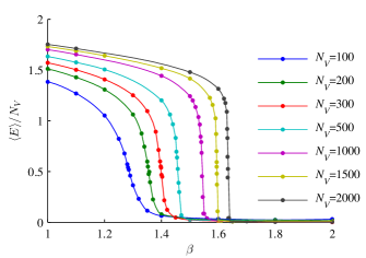
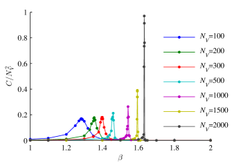
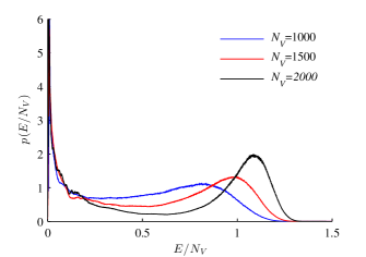
The results are shown in Fig. 6 and Fig. 7. For the three largest systems with $N_{V}=1000$, $N_{V}=1500$, and $N_{V}=2000$, we also employ the weighted histogram analysis method (WHAM) Ferrenberg and Swendsen (1988) to improve the sampling quality. The inverse transition temperature $\beta_{c}$ is defined as the inverse temperature where the heat capacity is maximal. It can be seen that $\beta_{c}$ increases as $N_{V}$ increases, an effect also seen previously in other graph models Konopka (2008); Conrady (2011) Near the transition temperature $\beta_{c}$, $|d\left\langle E\right\rangle/d\beta|$ also increases as $N_{V}$ increases, and thus the widths of the heat capacity peaks decrease as $N_{V}$ increases, indicating the transition becomes more cooperative. Figure 8 shows a log-log plot of the inverse transition temperature as a function of $N_{V}$. The linear relation in the plot indicates that as $N_{V}$ goes to infinity, the transition temperature would go to zero. In addition, Fig. 9 shows the probability density distribution of $E/N_{V}$, for the systems of size $N_{V}=1000$, $1500$, and $2000$, at each system’s transition temperature. As $N_{V}$ increases, the energy distribution of the two phases become more bimodal, and the temperature-dependence of the heat capacity in Fig. 6 becomes sharper, indicating a more cooperative transition with increasing system size Plotkin and Onuchic (2002a, b). Together this implies that the transition is first order in the bulk limit, with a corresponding nucleation barrier Binder (1987). That is, a Landau functional using system energy as an effective order parameter has a double-well structure with corresponding barrier separating the low- and high-energy phases Plischke and Bergersen (2006).

In appendix B, we give the acceptance ratio in our simulations as a function of inverse temperature. Although the acceptance ratio substantially decreases in the low-energy phase, the system is still able to undergo dynamics because some local defects cost little or no energy.

A transition temperature of zero for infinitely large graphs is actually not very surprising on entropic grounds. Consider a first order phase transition of an extended physics model. Denote the size of the system by $N$, and denote the number of states in the high- and low-temperature phases by $\Omega_{\textrm{H}}$ and $\Omega_{\textrm{L}}$, respectively. Because the energy difference between these two phases is proportional to $N$, the phase transition temperature $T_{c}$ is given approximately by $\Omega_{\textrm{H}}e^{-\kappa N/T_{c}}=\Omega_{\textrm{L}}$, where $\kappa$ is a positive number. As $N$ increases, for a “typical” physics system with short-ranged interactions, the ratio between $\Omega_{\textrm{H}}$ and $\Omega_{\textrm{L}}$ increases as $e^{\gamma N}$, where $\gamma$ is a positive number. This behavior results in a finite, nonzero transition temperature in the infinite size limit. On the other hand, the number of inequivalent graphs with $N_{V}$ vertices is typically $N_{V}^{\gamma^{\prime}N_{V}}$, (for example, see Erdős and Rényi (1959); Bender and Canfield (1978); Konopka (2008)) where $\gamma^{\prime}$ is a positive number that depends on the constraints of the allowed graphs. In our case, the allowed graphs should have every vertex valency equal to six or seven, and every vertex neighborhood should be connected. While we do not have an algorithm to count the exact number of allowed graphs, it is reasonable to assume for our system that the ratio between $\Omega_{\textrm{H}}$ and $\Omega_{\textrm{L}}$ has the typical asymptotic behavior of graphs, which explains a transition temperature of zero, i.e., the transition temperature $T_{c}$ is given by $N_{V}^{\gamma^{\prime}N_{V}}e^{-\kappa N_{V}/T_{c}}\approx 1$.

Figure 10: The entropy density difference across the transition $\Delta S/N_{V}$ as a function of $N_{V}$. The best fit line using a logarithmic function is also shown. The inset shows $\Delta S/N_{V}$ as a function of $N_{V}$ for a model including a Coulomb potential between valency-7 vertices (see section V). Including long-range interactions can remove super-extensivity of the entropy.

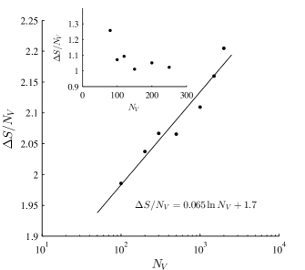
To validate the above argument, we can calculate the entropy difference across the transition as given by

$$\Delta S=\int_{T_{2}}^{T_{1}}\frac{C(T)}{T}dT=\int_{\beta_{1}}^{\beta_{2}}\frac{C(\beta)}{\beta}d\beta,$$ (7)

where $C$ is the heat capacity, and $\beta_{1}$ and $\beta_{2}$ are typical inverse temperatures in the high-temperature phase and low-temperature phase, respectively, which are taken to be $\beta_{1}=\beta_{c}-100/N_{V}$, $\beta_{2}=\beta_{c}+100/N_{V}$, i.e., we ensure that the window defining the transition narrows as the width of the heat capacity peak narrows. Fig 10 shows the difference in entropy density $\Delta S/N_{V}$ as a function of $N_{V}$, which, rather than remaining constant, is a monotonically increasing function. Thus the entropy of the system is super-extensive. If the ratio $\Omega_{\textrm{H}}/\Omega_{\textrm{L}}$ of the model scales like $N_{V}^{\gamma^{\prime}N_{V}}$ as argued above, $\Delta S/N_{V}$ will have the form $\Delta S/N_{V}=\gamma^{\prime}\ln N_{V}+b$. The best fit line using this logarithmic function is also shown in Fig 10, which is consistent with a super-extensive entropy, with $\gamma^{\prime}\simeq 0.065$.

IV.4 Geometric properties

In this sub-section, we analyze some geometric properties of the two phases: if a geometric property is distinct in the two phases, it can serve as an order parameter that signals the phase transition.

Figure 11: (Color online) Distribution of edge valencies as a function of inverse temperature $\beta_{c}$, for the system of size $N_{V}=1000$. There are no edges in the simulation with edge valency less than one or larger than five.

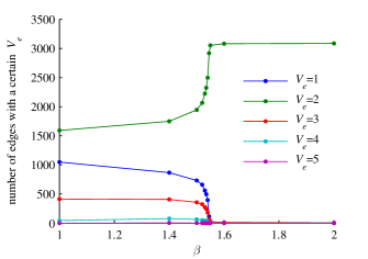
As was mentioned before, because the low-energy graphs are nearly triangulations for our Hamiltonian, it is useful to introduce an order parameter that measures how similar graphs are to triangulations. For this purpose we can study the distribution of edge valencies, where the edge valency is defined as the number of triangles that an edge is part of. In a perfect triangulation of a surface without boundaries, the edge valencies are always two, so we expect that at low temperatures, the distribution of edge valency should approximate a delta function around two. The distribution of edge valencies for the system of size $N_{V}=1000,X=100$ is shown in Fig. 11 as a function of temperature. Indeed, almost all edges have edge valency two at temperatures below the transition temperature. Near the transition temperature however, there is a sudden change in the distribution of edge valencies: above the transition temperature, edge valencies both above and less than two appear.

Figure 12: Average distance $\left\langle\bar{d}\right\rangle$ between pairs of vertices, plotted as a function of inverse temperature $\beta$, for the system of size $N_{V}=1000$. $\left\langle\bar{d}\right\rangle$ is first averaged over all pairs of vertices in a given snapshot, and then averaged over all snapshots at a given temperature. The vertical bars at each data point indicate the standard deviation between snapshots: $\sqrt{\left\langle\bar{d}^{2}\right\rangle-\left\langle\bar{d}\right\rangle^{2}}$.

Another quantity that is useful as an order parameter is the average distance between all pairs of vertices, denoted by $\left\langle\bar{d}\right\rangle$, where the bar means averaging over all pairs of vertices in a graph, and the angle bracket means averaging over samples of an equilibrium simulation. We expect that above the phase transition temperature, graphs will exhibit “small world” topologies and thus $\left\langle\bar{d}\right\rangle$ will be relativity small. The quantity $\left\langle\bar{d}\right\rangle$ gives the characteristic linear size of the graphs. Figure 12 plots $\left\langle\bar{d}\right\rangle$ vs. inverse temperature $\beta$, for $N_{V}=1000$. Indeed, the low-temperature phase has a larger $\left\langle\bar{d}\right\rangle$ than the high-temperature phase; low-temperature graphs tend to have much more structure than high-temperature graphs, resulting in larger values of $\left\langle\bar{d}\right\rangle$.

Figure 13: (Color online) The average distance $\left\langle\bar{d}\right\rangle$ between pairs of vertices as a function of the system size $N_{V}$ (discrete points), and the best fit lines using a square root function (green dashed lines), using a power function (red solid lines), and using a logarithmic function (black solid lines). Plots are shown both above the transition ($\beta=1.0$) in panel (a), and below the transition ($\beta=2.0$) in panel (b). For each best fit line, its expression and $p$-value are also shown, where the $p$-values are calculated for the null hypothesis that the residues $(d_{\textrm{fit}}-\left\langle\bar{d}\right\rangle)/\delta d$ come from a normal distribution with variance smaller than 1. For both temperatures, the logarithmic function gives the best fit to the measured data.

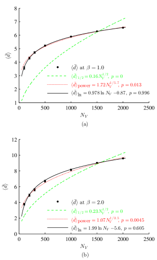
In Fig. 13, the average distance $\left\langle\bar{d}\right\rangle$ is shown as a function of the system size $N_{V}$, at $\beta=1.0$ (above the transition) and at $\beta=2.0$ (below the transition). The best fit lines using a logarithmic function and using a power function are also shown in Fig. 13. The $p$-value for each best fit line is calculated for the null hypothesis that the residues $(d_{\textrm{fit}}-\left\langle\bar{d}\right\rangle)/\delta d$ come from a normal distribution with variance smaller than 1, so that a higher $p$-value indicates a better model. These relations between $\left\langle\bar{d}\right\rangle$ and $N_{V}$ can be understood by comparing with random graphs, which generally display “small-world” connectivity, with average distances growing logarithmically with the number of vertices Erdős and Rényi (1959). In our model, the Hamiltonian only constrains the graphs locally, so these graphs satisfy small-world behavior in the high temperature phase accurately, as shown by the logarithmic best fit line in Fig. 13(a). For the low temperature phase, we can define an effective scaling dimension (see, e.g., Creswick et al. (1992))

$$D_{s}=\frac{d\ln N_{V}}{d\ln\left\langle\bar{d}\right\rangle}.$$ (8)

On a non-fractal surface, $\left\langle\bar{d}\right\rangle\sim N_{v}^{1/2}$, i.e., $D_{s}=2$. However, it is seen from Fig. 13(b) that the residuals with the square root function are too large. If we take $D_{s}$ as a parameter in the fitting, a power-law function with $D_{s}\simeq 3.5$ is a much better fit to the empirical scaling. Perhaps surprisingly however, the logarithmic function is still the best fit function, indicating that the low-temperature graphs still display small-world connectivity. Enforcing a power-law fit at every system size, i.e., $\left\langle\bar{d}\right\rangle\sim N_{v}^{1/D_{s}\left(N_{v}\right)}$, would induce a variable dimensionality in the exponent.

Figure 14: (Color online) Log-log plot of $\left\langle\bar{N}_{r}\right\rangle$, the thermally averaged number of vertices within a distance $r$, as a function of $r$; the slope gives the dimensionality of the system, which in this case is distance-dependent. The plot shown is for the system with size $N_{V}=2000$, at $\beta=1.0$ (blue line) and at $\beta=2.0$ (red line), which bracket the transition. For the same system, the inset shows the fractal dimension as a function of $r$.

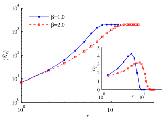
Another related definition of dimensionality measures the increase in number of vertices with distance from a given vertex. On a graph, one can pick an arbitrary central vertex, and count how many vertices $N_{r}$ have distance no greater than $r$ from that center. We can then average both over all central vertices and over all equilibrium configurations at a given temperature, denoting the doubly averaged volume by $\left\langle\bar{N}_{r}\right\rangle$. If $\left\langle\bar{N}_{r}\right\rangle$ increases with $r$ polynomially, the fractal (Haussdorf) dimension can be defined as

$$D_{f}=\frac{d\ln\left\langle\bar{N}_{r}\right\rangle}{d\ln r}.$$ (9)

In practice the dimension of the graph may itself depend on the radius $r$, so it makes sense to talk rigorously about the dimensionality of a graph only if $D_{f}$ is essentially constant over some range of $r$. A log-log plot of $\left\langle\bar{N}_{r}\right\rangle$ vs. $r$ is shown in Fig. 14, for $N_{V}=2000$ at $\beta=1.0$ and $\beta=2.0$, where the slope thus gives the dimensionality and is shown in the inset. One can see that the effective dimension $D_{f}$ is smaller below the transition. Consistent with the previous analysis using (8), there is no well-defined dimension for the graphs, which are small-world-like. Instead there is an increasing dimensionality with increasing length scale, until boundary effects of the system are felt. The dimensionality has values around 2 for small values of $r$, because of the local lattice-like structure; it is also small for very large values of $r$, because a finite-sized graph must eventually be bounded, at which point $\left\langle\bar{N}_{r}\right\rangle$ will no longer increase polynomially at large $r$. Table 1 lists the maximal value of $D_{f}(r)$ for systems with different sizes, at inverse temperatures $\beta=1.0$ and $\beta=2.0$. As the table shows, $D_{f,\textrm{max}}$ increases with $N_{V}$, which indicates that as $N_{V}$ increases, there is no universal fractal dimensionality that can be approached by the graphs. Instead, the graphs are still small-world.

	$\beta=1.0$	$\beta=2.0$
$N_{V}=1000$	$3.62$	$2.72$
$N_{V}=1500$	$3.99$	$3.11$
$N_{V}=2000$	$4.26$	$3.20$

Table 1: The maximal value of the fractal dimension $D_{f}$ as defined in (9) for systems with $N_{V}=1000$, $N_{V}=1500$ and $N_{V}=2000$, at inverse temperatures $\beta=1.0$ above the transition and $\beta=2.0$ below the transition.

The small-worldness of the low temperature graphs in the bulk limit can be viewed as a consequence of the graph Hamiltonian in (5), which is a sum of local terms. The defects in the manifold are also local — in the bulk these have no effect on the large-scale structure of the resulting graphs. This is manifested for finite-size graphs by the fact that as $N_{V}$ increases, the topologies of graphs become progressively more complicated, see e.g. Fig. 4(c) and Fig. 4(d). The manifolds contain numerous handles and surface intersections, so that a planar dimensionality does not adequately describe the system. In this sense there is already the signature in the low-temperature phase of the finite system that the bulk system is always disordered.

IV.5 Correlation functions

Figure 15: (Color online) Radial correlation function defined through (10) of (a) valency-7 vertices and (b) valency-3 edges. Correlations are calculated for the system with size $N_{V}=2000$ at $\beta=1.62$, which is in the high-temperature phase, and at $\beta=1.65$, which is the low-temperature phase.

Defects in this model such as those shown in Fig. 5 contain irregularities that make them differ from part of a regular lattice. However, regions far away from them may not be affected by their existence; i.e., there may be no long-range correlation between such defects. In this subsection, we define and calculate correlation functions between defect pairs.

Because valency-7 vertices induce defects, we first measure the radial correlation function of valency-7 vertices. In general, the correlation between two random variables $X,Y$ with expected values $\mu_{X},\mu_{Y}$ and standard deviations $\sigma_{X},\sigma_{Y}$ is defined as

$$\textrm{corr}(X,Y)=\frac{E[(X-\mu_{X})(Y-\mu_{Y})]}{\sigma_{X}\sigma_{Y}},$$ (10)

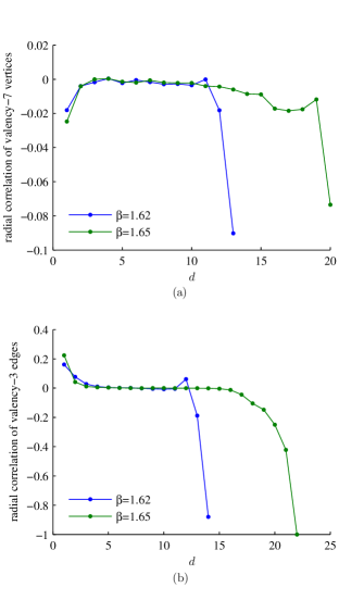
where $E$ is the expectation value operator. In our case, we take all pairs of vertices with distance $d$ in a graph; $X$ is 1 if the first vertex in a pair has valency 7, and 0 otherwise, and $Y$ is defined similarly for the second vertex. Then the correlation function is averaged over all equilibrium samples. The result for $N_{V}=2000$, taken at inverse temperatures $\beta=1.62$ and $\beta=1.65$, which are marginally below and above $\beta_{c}$ respectively, is shown in Fig. 15(a). When the distance $d$ is very small ($d=1$ or $2$), the correlation function deviates from zero, because of the local structure of of the defects (see Fig. 5), which in this case induces anti-correlation. For intermediate values of $d$ ($3\leq d\leq 10$), the correlation is very small, indicating the defects are uncoupled. However, for large values of $d$, the correlation function becomes negative. This is because the valency of a vertex, and the distance from this vertex to other vertices, are not independent: compared with the valency-6 vertices, the valency-7 vertices tend to have smaller distances to other vertices. For example, for $N_{V}=2000,\beta=1.62$, the mean distance to valency 6 vertices is 7.18, while the mean distance to valency 7 vertices is 7.04. Thus it is less probable to find two valency-7 vertices with a large distance, and hence they anti-correlate at large distances. The correlation function is quite small over a range of $d$ as one might anticipate, but the above global effect makes it difficult to quantitatively confirm that defects are decoupled at large distance.

As another measure of the correlation between defects, we can measure the radial correlation function of valency-3 edges, since their existence indicates deviation of the graph from a triangulation of surface. For example, every defect in Fig. 5 contains valency-3 edges. The distance between two edges is defined by taking the 4 vertices defining the two edges, and finding the pair of vertices with the minimum distance between them. Since a pair of edges having a common vertex would then have a distance of zero, we add one to the above definition of edge distance. The results for $N_{V}=2000$, at $\beta=1.62$ and $\beta=1.65$, are shown in Fig. 15(b). At small distances ($d\leq 3$), there exists short range positive correlation between the valency-3 edges — the mean force between them is attractive, due again to the particular structure within a given low energy local defect. At large distances ($d\geq 14$ for $\beta=1.62$, $d\geq 17$ for $\beta=1.65$), the correlation function becomes negative, because valency-3 edges correlate with valency-7 vertices, which in turn anti-correlate at large distances for the reasons described above. However for a wide range of intermediate distances, this correlation function is also nearly zero, indicating again that the defect attraction is short-ranged.

V Addition of a Coulomb potential

We found above that as the graph size $N_{V}$ increased to infinity, the transition temperature $T_{c}$ approached zero (Fig. 8). This is apparently a universal property of models based on graphs, due to the super-extensive entropy of the high-temperature random phase. Similar arguments appear in the theory of phase transitions of low-dimensional systems Landau and Lifshitz (1958), wherein the non-extensive energy cost of defect formation is outweighed at any nonzero temperature by the (extensive) free energy due to translational entropic gain, so long as interactions are sufficiently short-ranged. This analogy motivated us to introduce a model with long-ranged interactions between defects, anticipating that in such a defect-filled system incurs super-extensive energetic cost, which may in turn result in a nonzero transition temperature.

Thus, in addition to the original two terms in the Hamiltonian (5), we introduce a nonlocal Coulomb potential term to the Hamiltonian, which gives a repulsive force between any pair of degree-7 vertices,

$$H_{3}=c_{3}\sum_{v,u\in V(G),v\neq u}\frac{\delta_{n_{v},7}\delta_{n_{u},7}}{d(v,u)}.$$ (11)

This is one of the simplest non-local Hamiltonian terms that one can add to the original Hamiltonian. The Coulomb force is chosen to be repulsive, because most of the high-temperature states are “small world”, in that they have smaller average distances than those of low temperature states, so such a Coulomb potential can suppress the appearance of these “small world” graphs.

Figure 16: (Color online) Sample configurations for the model with Coulomb potential in (11) with $c_{3}=1.0$, for the system with number of vertices $N_{V}=200$ and number of extra edges $X=20$, drawn in three dimensions. Panel (a) shows a typical configuration in the high-temperature phase with $\beta=1.0$; panel (b) shows a typical configuration in the low-temperature phase with $\beta=2.0$.

Figure 17: (Color online) Log-log plot of transition temperatures $\beta_{c}$ as a function of system size $N_{V}$, for the model with local Hamiltonian in (5) (drawn as circles, with best fit drawn as solid line), and for the model with Coulomb potential in (11) with $c_{3}=1.0$ added to the local Hamiltonian (discrete points with error bars). The inset shows the rescaled heat capacity $C/N_{V}$ as a function of inverse temperature $\beta$ for systems with the Coulomb potential added, and from which the values and uncertainties of $\beta_{c}$ values are determined.

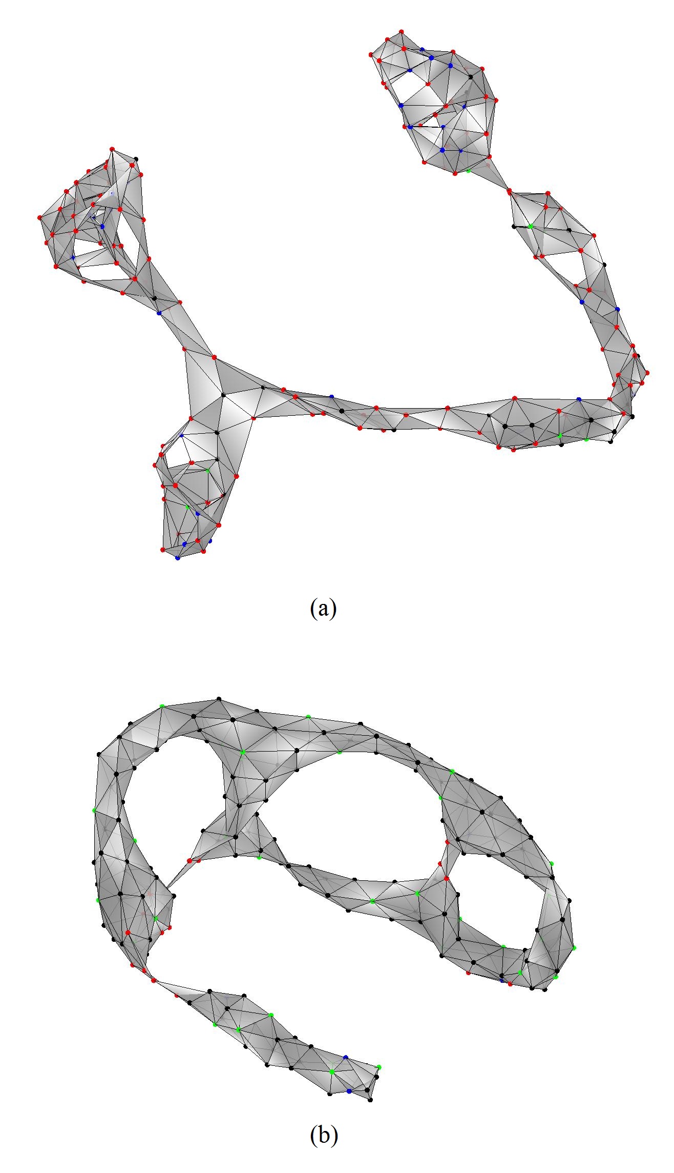
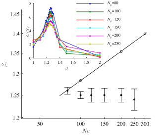
We test the effect of addition of this Coulomb term by another set of simulations, in which $c_{3}=1.0$. Figure 16 shows the sample drawings of graphs with $N_{V}=200,X=20$ (a) at high temperature ($\beta=1.0$) and (b) at low temperature ($\beta=2.0$). These temperatures bracket the heat capacity peak for the system so that the system is in the disordered and ordered phases respectively (Fig. 17). Because of the non-locality of $H_{3}$, simulations are much slower in practice than before and smaller systems are thus employed: simulations are performed for $N_{V}=80,100,120,150,200$ and $250$, and $X=0.1N_{V}$. The inset of Fig. 17 shows the rescaled heat capacity $C/N_{V}$ as a function of $\beta$, for several system sizes. The rescaling factor is now chosen differently than in Fig. 7, because the systems with the Coulomb potential have maximal heat capacity approximately proportional to $N_{V}$. From the maximal heat capacity, the inverse transition temperature $\beta_{c}$ is determined, and is shown in Fig. 17 (main panel), in comparison with the $\beta_{c}$ values without the Coulomb potential.

From the graph drawings in Fig. 16, we can see that because of the repulsive Coulomb force, both the high-temperature and low-temperature manifold configurations become rather extended to achieve longer average distances between defects. This may also explain why the transition temperature does not change very much with $N_{V}$: The characteristic linear size of the systems is much larger when the repulsive Coulomb potential is present, which penalizes the increase in complexity that was observed for a local Hamiltonian as $N_{V}$ increased. We thus suspect that the entropy would be extensive for the long-ranged interaction model. To quantify this, as a final check we plot the entropy change between disordered and ordered phases as a function of $N_{V}$ in the inset of Fig. 10, where $\Delta S$ is calculated by Equation (7), and $\beta_{1}=1.0$, $\beta_{2}=2.0$. As opposed to the entropy difference in the original model, $\Delta S/N_{V}$ of this model is approximately constant as $N_{V}$ increases, i.e. the entropy difference is no longer super-extensive, rather it is extensive or sub-extensive.

Figure 18: (Color online) Sample configurations for the model with Coulomb potential in (11) with $c_{3}=-1.0$, for the system of size $N_{V}=200,X=20$ drawn in three dimensions. Panel (a) shows a typical configuration in the high-temperature phase with $\beta=1.0$; panel (b) shows a typical configuration in the low-temperature phase with $\beta=2.0$.

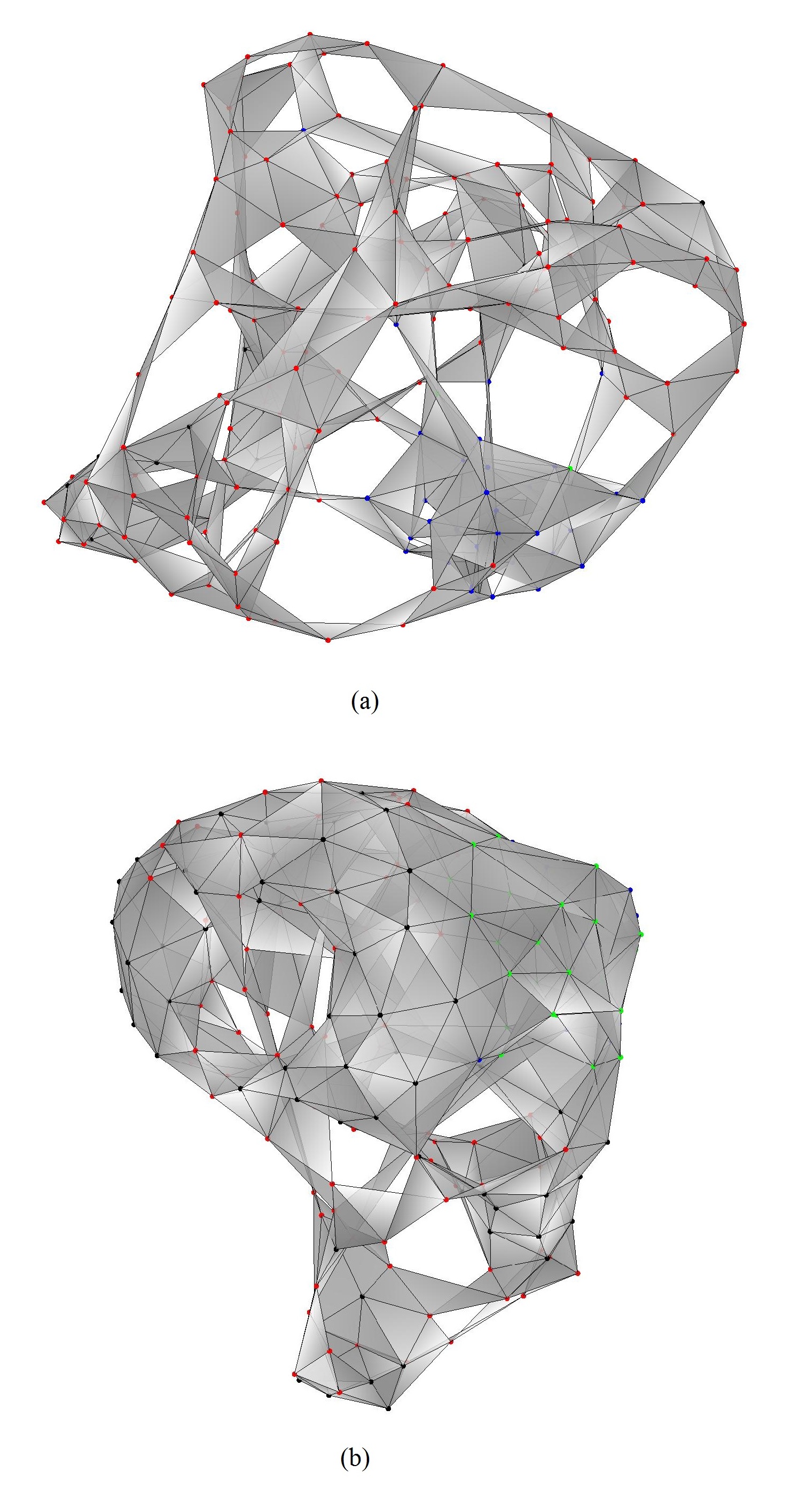
We also simulate the model with an attractive Coulomb potential, in which $c_{3}=-1.0$. Figure 18 shows sample drawings of graphs with $N_{V}=200,X=20$ (a) at high temperature ($\beta=1.0$) and (b) at low temperature ($\beta=2.0$). The effect of the attractive potential can be observed in these samples, in that the valency-7 vertices (green and blue dots) are usually located close together. In addition, because a local move must involve a valency-7 vertex, the configuration cannot evolve in the regions composed of purely valency-6 vertices, and thus the simulation is inefficient. As can be seen in Fig. 18(b), in the region of valency-6 vertices, the configuration does not minimize the Hamiltonian (red dots have positive contribution to $H_{2}$), and is not a triangulation. Thus Fig. 18(b) depicts a long-lived meta-stable state on an energy landscape of states characteristic of a frustrated system Plotkin and Onuchic (2002a, b). Such a model has numerous local minima with large reconfigurational barriers between them, and consequently glassy relaxation dynamics.

VI Discussion

In this paper we have constructed a graph model with a local Hamiltonian that simply enforces minimal valency subject to a given total number of graph links, along with a graph symmetry between the local graph radius and diameter. The above minimal condition along with fixed total link number gives rise to near constant valency for all vertices. This Hamiltonian gives rise to an emergent manifold at low temperature. The one free parameter in the model does not appear in the Hamiltonian but as an initial condition of the system. This parameter $\alpha$ determines the edge to vertex ratio, which is conserved for the system and determines the dimensionality of the emergent manifold. When $\alpha$ is slightly larger than 6, the low temperature solutions have structural properties consistent with triangulations of two-dimensional surfaces. We obtained a representation of the emergent manifold by an optimization scheme, wherein adjacent vertices are brought as close as possible to a certain link distance, non-adjacent vertices are repelled from each other, and every triangular subgraph is assumed to be filled to render the manifold.

The spacetime manifold has historically been treated as a triangulation in several previous approaches, in order to regularize the partition function by constructing discrete analogs to the continuum manifold Weingarten (1982); David (1985); Ambjorn et al. (1985); Kazakov et al. (1985); Boulatov et al. (1986). For example, in dynamical triangulation theory a given spacetime manifold is triangulated by simplices to calculate a discretized gravitational action Johnston (1997); Bowick (1998); Ambjørn et al. (2005a). In matrix models of gravity, graphs may be constructed as dual to Feynman diagrams arising from the limit of large internal symmetry group; by construction the graph constitutes a manifold. The partition function for two-dimensional quantum gravity can be expressed as a sum over topologies of triangulated 2D surfaces, for actions of various forms describing the coupling between matter fields and spacetime Di Francesco et al. (1995); this problem has connections to string theory via the Polyakov action Polyakov (1981). The formalism may be extended to study higher dimensional generalizations of quantum gravity by group field theory models Oriti (2006). In this context, the emergence of a smooth “hydrodynamic” spacetime has been described as a condensation of simplicial quantum building blocks Oriti (2007). Such dual graph triangulations have widely varying vertex valency but generally represent manifold-like surfaces, at least in the condensed phase. In contrast, the emergent manifolds that we observe have near constant valency, but often bifurcating morphologies, e.g. the “bubble-wrap” or “frenulum” defects in Fig. 5.

Figure 19: (Color online) (a) A 3D cube triangulated into 5 tetrahedra  Üngör (2001) may be replicated by translation and reflection to tesselate the 3D space. Here, part of the dual lattice is shown as well in red. Red vertices are at the centers of the tetrahedra in the original triangulation. At the sites where the dual lattice bonds pass through the faces of tetrehedra in the original tesselation, open circles are drawn. (b) 3D Euclidean space subdivided into the cubes shown in panel (a) (grey lines); triangulation of the cubes in panel (a) is not shown explictly here. The thicker black lines correspond to the dual graph of this triangulation.

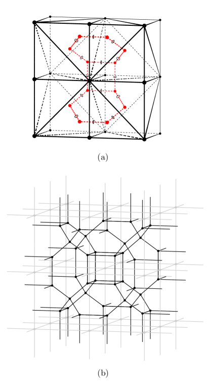
One can ask whether the present graph model could act as a substitute for the Feynman diagram construction in matrix models. The Feynman diagram construction has fixed valency, and is dual to a triangulated manifold, so a graph model of nearly fixed valency $n_{v}$ could in principle give rise to an emergent manifold of dimensionality $n_{v}-1$ as its dual. The present graph-symmetry-based Hamiltonian, and the resulting triangular lattice-like graphs in the low temperature phase, make this interpretation unlikely. The mean valency in the low temperature phase of our graph model is approximately 6, corresponding to the triangular lattice graph; we thus may consider a tesselation of a five-dimensional Euclidean space by tetrahedra. The triangular lattice graph has smallest cycles of 3 vertices, corresponding to traversing the smallest triangles in the graph. However, a Euclidean tesselation using non-obtuse simplices will have cycles of its dual graph with no less than 4 vertices, i.e. due to the acuteness (or more precisely non-obtuseness) of the simplices, every cycle consists of a (potentially non-planar) polygon of at least 4 sides. As an illustration of this, consider the dual graph to a three-dimensional tesselation by tetrahedra with non-obtuse dihedral angles. A section of a three-dimensional tiling by such tetrahedra is shown in Fig. 19(a), and the corresponding dual graph is shown in Fig. 19(b). Here we see that the smallest cycles of the dual graph are indeed 4, corresponding to $\pi/2$ dihedral angles of the tiling tetrahedra. However a significant fraction of the cycles have length 6. Moreover, the cycles of length 4 appear as faces of 3D cubes in the dual lattice. All of this structure is incompatible with a regular planar graph of valency 4 as a potential dual to the three-dimensional tesselation; in particular, a graph having the topology of a square lattice is ruled out.

In the model, there are no constraints on the global structure of the graph. As a consequence, the low-temperature phase can still retain complicated topologies with small-world properties, for which the corresponding manifold shows handles, self-intersections, and local defects that deviate from the manifold, in that a higher embedding dimension is necessary to represent them. Defects on the low-temperature manifold induce scattering and lensing effects on the propagation of bosonic matter fields Quach et al. (2012), and are an interesting topic of future work for our model. As well, the presence of non-local links in the low temperature graph, and the corresponding non-locality in the emergent manifold, is consistent with the possible presence of disordered locality in loop quantum gravity Markopoulou and Smolin (2007), and might constitute a mechanism for its generation. In the context of loop quantum gravity, macroscopic expectation values of area or volume deviate from those on a flat metric by $\mathcal{O}(\ell_{p}^{2})$ or $\mathcal{O}(\ell_{p}^{3})$ where $\ell_{p}$ is the Planck length; nonlocal connections in the underlying metric modify the local Hamiltonian coupling a matter field to loop quantum gravity, but leave the above expectation values essentially unchanged, indicating locality may be macroscopically smooth but microscopically disordered.

As a general property of the graph model, the high-temperature phase has an entropy that grows super-extensively with system size $N_{V}$. This results in a transition temperature of zero in the limit $N_{V}\rightarrow\infty$, so that the infinite manifold is always disordered at any finite temperature. Aside from a finite universe or diverging coupling constraints as possible solutions, we implemented long-range interactions between vertex defects with repulsive Coulombic potential, to energetically penalize the many graph configurations with defect arrangements consistent with small-world topologies. In analogy with low-dimensional condensed matter systems, long-range potentials that couple defects induce prohibitive energetic cost to configurations that would otherwise destroy order entropically, so that an ordered phase at low temperature is restored. Here, we found that such potentials result in a nearly constant transition temperature as the size of the graph $N_{V}$ increases. In addition, we found that attractive Coulombic potentials result in long-lived metastable states in the simulations.

Another interesting feature of the model is that the low lying energy levels, including the ground state level, have large configurational degeneracy. This residual entropy is due to local defects that can “absorb” extra edges without energetic cost. As well, the simulation dynamics indicates that the energy barriers between different low-energy states are not high. Thus at temperatures below the phase transition, the degrees of freedom in the system arising from this residual entropy are not frozen. The small or zero-energy barriers between degenerate states make the low-temperature graph system similar to the spin ices observed in spinel structures and pyrochlore lattices Pauling (1935); Anderson (1956); Bramwell and Gingras (2001).

We have implemented here a sufficiently general Hamiltonian such that the same dynamic model can give rise to space-times of different dimensionality, i.e. spaces of different dimensions are solutions to the same model. Exclusively from the graph theory point of view, there is no a priori reason to choose any particular dimensionality as a phenomenological term in the Hamiltonian. The “emergent dimensionality”, then comes from initial conditions. Our motivation for this was to choose the simplest Hamiltonian possible, that was free of phenomenological parameters, so that the dimensionality of space-time was not “baked into” the energy function that governed dynamics. That said, we acknowledge that this approach effectively shifts the space-time dimension from extra phenomenological parameters in the Hamiltonian that favor or disfavor particular subgraphs Conrady (2011), to special initial conditions. Our Hamiltonian is local in that it is a sum over all the vertices, and each term only depends on a small neighborhood (in our case, the neighborhood subgraph) of each vertex. This contrasts with other quantum graphity Hamiltonians, which have actions that depend on the number of loops with long lengths Konopka et al. (2008).

It is intriguing to interpret the low-temperature configurations of this graph model as an emergent spacetime — a notion other researchers have explored for similar graph models Ambjørn et al. (2004, 2005a); Konopka et al. (2006, 2008); Konopka (2008); Hamma et al. (2010); Caravelli et al. (2012); Conrady (2011); Caravelli and Markopoulou (2011). In this picture, general relativity is an effective “hydrodynamic” theory emerging from the collective dynamics of more fundamental degrees of freedom. The graph model is appealing in that both spacetime manifolds and locality emerge in the low-temperature regime of a discrete structure. The graph model introduced here gives rise to real, positive distances, so the emergent manifold can only be a Wick-rotated, Euclidean version of spacetime. Monte Carlo “time” steps in the current Hamiltonian methodology are distinct from the time evolution of the graph or manifold, and are only a mechanism to sample equilibrium states. In the present formulation, the Euclidean gravity theory undergoes a phase transition to smooth metrics below a “temperature” parameter $\beta$. Exploiting the isomorphism between the quantum propagator and the statistical mechanical partition function Kogut (1979), the quantity $\mbox{e}^{-\beta\cal{H}}/\int[dg]\mbox{e}^{-\beta\cal{H}}$ is the equivalent to the Euclidean path integral measure that determines Green functions $\left<g_{1}\ldots g_{n}\right>$ for the metric $g$ in a quantum gravity model with the corresponding action. While we have seen a phase transition for the system with Euclideanized action, the identification of the appropriate thermal quantum states that are periodic in real time, and so related to the parameter $\beta$, is not clear at present. We see this problem of mapping back to the space-time coordinates with Minkowskian signature as a general challenge for quantum graphity models. Another general issue is the absence of an underlying symmetry principle to determine the action in quantum graphity models, analogous to the role of general covariance in the action for quantum gravity.

The complex topologies of surfaces corresponding to low-temperature graphs, along with graph defects having zero energetic cost, implies that a graph model consisting solely of the current Hamiltonian does not reduce to a classical theory of Euclidean gravity in the macroscopic limit. On the other hand, other discrete models of gravity are also known to have scale-dependent spectral dimension, indicating fractal, non-smooth geometries for the emergent manifolds at least at intermediate length scales Ambjørn et al. (1995, 2005b); Giasemidis et al. (2012). The set of all possible low-energy graphs in this model could potentially be identified with the phase space of a Euclidean gravity theory before imposing the equation of motion, i.e., the space of all possible metrics modulo diffeomorphisms. Because the low-temperature graphs of our model are nearly triangulations, and random triangulations form the phase space of many other discrete gravity models Di Francesco et al. (1995); Johnston (1997); Bowick (1998); Ambjørn et al. (2005a); Oriti (2006), it may be interesting to investigate whether the graph model’s action may be extended to include terms in dynamical triangulation theory, which do reduce to the gravitational action in the continuous limit.

The transition from disordered to ordered manifolds is first-order in the present graph model. However, the order of the transition, and its potential relevance to universality or independence of underlying lattice specifics, is a non-issue for the investigation of ordered phases below the transition, where correlation lengths are finite. Power-law correlations calculated in causal dynamical triangulation are between graphical elements analogous to graviton fields, so that graviton coupling is power law as in the classical limit. Space to time ratios of simplices have second order transition in this model, while the transition involving gravitational coupling is first order Ambjørn et al. (2011). In any event, a graph model at a critical point would have wildly fluctuating connectivity and resemble more a fractal mix of ordered and disordered states, which is not consistent with an emergent manifold. The issue of the universality classes and corresponding exponents of a transition is a separate one from the properties of an emergent manifold as a low-temperature phase below a phase transition. Retention of microscopic structure in the disorder to order transition is a prediction of the graph model, and may enable future experimental tests.

Finally, it is intriguing to speculate on the utility of a such a graph theoretical transition to describe a transition involving non-local to local causality, as might occur in a pre-inflationary universe. Such models may address the low-entropy initial condition problems that occur in inflationary models Penrose (1989); Carroll and Chen (2005).

Appendix A The weighted histogram analysis method

The weighted histogram analysis method (WHAM) is a method to combine the samples from several Monte Carlo simulations taken under conditions of different temperature and added potential. We employ WHAM to generate optimal estimates of energy distributions of the graph model. In this model, the energy takes only integer values between $0$ and $M=1.5N_{V}$. Assume that $S$ simulations are performed (in our cases, $S=4$ for $N_{V}=1000$, $S=10$ for $N_{V}=2000$), with inverse temperature $\beta_{i}$, and biasing potential $V_{i}(E)$, i.e., in the $i$-th simulation, the system is sampled with energy distribution $\Omega(E)\exp(-\beta_{i}(E+V_{i}(E)))$, where $\Omega(E)$ is the yet-unknown number of states with energy $E$. The inverse temperature $\beta_{i}$’s are taken to be near the inverse transition temperature. Because there is a large free energy barrier between the low and high energy phases near the transition temperature, a biasing potential is used to obtain better sampling in the barrier region. The form of the biasing potential is taken to be parabolic:

$$V_{i}(E)=\left\{\begin{array}[]{ll}v_{i}\left[\frac{\left(E-\frac{E_{i}^{l}+E_{i}^{h}}{2}\right)^{2}}{\left(\frac{E_{i}^{h}-E_{i}^{l}}{2}\right)^{2}}-1\right],&E_{i}^{l}\leq E\leq E_{i}^{h},\\ 0,&E<E_{i}^{l},\\ 0,&E>E_{i}^{h},\end{array}\right.$$

where the parameters $v_{i}$, $E_{i}^{l}$ and $E_{i}^{h}$ are chosen by trial and error to make the energy distribution of each simulation as flat as possible.

After performing the simulations, let $n_{i}(E)$ be the number of counts of energy $E$ from the $i$-th simulation, and $N_{i}$ the total number of samples from the $i$-th simulation. From this information, the optimal estimate of the probability $p^{0}(E)$ of energy level $E$ at inverse temperature $\beta^{0}$ without any biasing potential is given by

$$p^{0}(E)=\frac{\sum_{i=1}^{S}n_{i}(E)}{\sum_{i=1}^{S}N_{i}f_{i}c_{i}(E)},$$ (12)

where $c_{i}(E)$ is the biasing factor $c_{i}(E)=\exp[-(\beta_{i}-\beta^{0})E-\beta_{i}V(E)]$, and $f_{i}$ is a normalization constant satisfying

$$f_{i}^{-1}=\sum_{E=0}^{M}c_{i}(E)p^{0}(E).$$ (13)

To solve these equations, we take an arbitrary set of initial values for $f_{i}$ (namely $f_{i}^{0}=1$), and apply (12) and (13) iteratively to find the solution to these equations. After finding $p^{0}(E)$, it is then straightforward to calculate the average energy and heat capacity at inverse temperature $\beta^{0}$.

Appendix B Acceptance ratio

Figure 20: For the system of size $N_{V}=1000$, the acceptance ratio of Monte Carlo moves in the simulations is plotted as a function of inverse temperature $\beta$.

As a practical matter, we plot the acceptance ratio as a function of $\beta$ for $N_{V}=1000$ in Fig. 20. The low energy phase occupied at large values of $\beta$ has a much lower acceptance ratio than the high energy phase, both because of the lower temperature and because the low energy graphs have much more structural constraints, and thus have more rigidity with respect to the local moves. However, because some the local defects cost little or no energy, low energy graphs still have nonzero acceptance ratio, and so are able to undergo dynamics during the simulations.

References

- Erdős and Rényi (1959) P. Erdős and A. Rényi, Publicationes Mathematicae Debrecen 6, 290 (1959).
- ’t Hooft (1974) G. ’t Hooft, Nucl.Phys. B72, 461 (1974).
- Ambjørn et al. (2004) J. Ambjørn, J. Jurkiewicz, and R. Loll, Phys.Rev.Lett. 93, 131301 (2004), arXiv:hep-th/0404156 [hep-th] .
- Ambjørn et al. (2005a) J. Ambjørn, J. Jurkiewicz, and R. Loll, Phys.Rev. D72, 064014 (2005a), arXiv:hep-th/0505154 [hep-th] .
- Albert and Barabási (2002) R. Albert and A.-L. Barabási, Rev. Mod. Phys. 74, 47 (2002).
- Franzblau (1991) D. S. Franzblau, Phys. Rev. B 44, 4925 (1991).
- Bhalla and Iyengar (1999) U. S. Bhalla and R. Iyengar, Science 283, 381 (1999).
- Hopfield (1982) J. J. Hopfield, Proceedings of the National Academy of Sciences 79, 2554 (1982), http://www.pnas.org/content/79/8/2554.full.pdf+html .
- Konopka et al. (2006) T. Konopka, F. Markopoulou, and L. Smolin, (2006), arXiv:hep-th/0611197 [hep-th] .
- Konopka et al. (2008) T. Konopka, F. Markopoulou, and S. Severini, Phys. Rev. D77, 104029 (2008), arXiv:0801.0861 [hep-th] .
- Konopka (2008) T. Konopka, Phys.Rev. D78, 044032 (2008), arXiv:0805.2283 [hep-th] .
- Hamma et al. (2010) A. Hamma, F. Markopoulou, S. Lloyd, F. Caravelli, S. Severini, et al., Phys.Rev. D81, 104032 (2010), arXiv:0911.5075 [gr-qc] .
- Caravelli et al. (2012) F. Caravelli, A. Hamma, F. Markopoulou, and A. Riera, Phys.Rev. D85, 044046 (2012), arXiv:1108.2013 [hep-th] .
- Conrady (2011) F. Conrady, J. Statist. Phys. 142, 898 (2011), arXiv:1009.3195 [gr-qc] .
- Mermin and Wagner (1966) N. Mermin and H. Wagner, Phys.Rev.Lett. 17, 1133 (1966).
- Hohenberg (1967) P. Hohenberg, Phys.Rev. 158, 383 (1967).
- Coleman (1973) S. R. Coleman, Commun.Math.Phys. 31, 259 (1973).
- Malnič and Mohar (1992) A. Malnič and B. Mohar, J. Combin. Theory Ser. B 56, 147 (1992).
- Newman and Barkema (1999) M. E. G. Newman and G. T. Barkema, Monte Carlo methods in statistical physics (Clarendon Press, Oxford, 1999).
- Note (1) See Appendix A for the details of our implementation of WHAM.
- Ferrenberg and Swendsen (1988) A. M. Ferrenberg and R. H. Swendsen, Phys. Rev. Lett. 61, 2635 (1988).
- Plotkin and Onuchic (2002a) S. S. Plotkin and J. N. Onuchic, Quart. Rev. Biophys. 35, 111 (2002a).
- Plotkin and Onuchic (2002b) S. S. Plotkin and J. N. Onuchic, Quart. Rev. Biophys. 35, 205 (2002b).
- Binder (1987) K. Binder, Reports on Progress in Physics 50, 783 (1987).
- Plischke and Bergersen (2006) M. Plischke and B. Bergersen, Statistical Physics, 3rd ed. (World Scientific, Singapore, 2006).
- Bender and Canfield (1978) E. A. Bender and E. R. Canfield, J. Combinatorial Theory Ser. A 24, 296 (1978).
- Creswick et al. (1992) R. Creswick, H. Farach, and C. Poole, Introduction to renormalization group methods in physics, A Wiley-Interscience publication (Wiley, 1992).
- Landau and Lifshitz (1958) L. Landau and E. Lifshitz, Statistical physics, Addison-Wesley series in advanced physics (Pergamon Press, 1958).
- Weingarten (1982) D. Weingarten, Nucl.Phys. B210, 229 (1982).
- David (1985) F. David, Nucl.Phys. B257, 45 (1985).
- Ambjorn et al. (1985) J. Ambjorn, B. Durhuus, and J. Frohlich, Nucl.Phys. B257, 433 (1985).
- Kazakov et al. (1985) V. Kazakov, A. A. Migdal, and I. Kostov, Phys.Lett. B157, 295 (1985).
- Boulatov et al. (1986) D. Boulatov, V. Kazakov, A. A. Migdal, and I. Kostov, Phys.Lett. B174, 87 (1986).
- Johnston (1997) D. Johnston, Nucl.Phys.Proc.Suppl. 53, 43 (1997), arXiv:hep-lat/9607021 [hep-lat] .
- Bowick (1998) M. J. Bowick, Nucl.Phys.Proc.Suppl. 63, 77 (1998), arXiv:hep-lat/9710005 [hep-lat] .
- Di Francesco et al. (1995) P. Di Francesco, P. H. Ginsparg, and J. Zinn-Justin, Phys.Rept. 254, 1 (1995), arXiv:hep-th/9306153 [hep-th] .
- Polyakov (1981) A. M. Polyakov, Phys.Lett. B103, 207 (1981).
- Oriti (2006) D. Oriti, “The Group field theory approach to quantum gravity,” in Approaches to Quantum Gravity (Cambridge University Press, 2006) arXiv:gr-qc/0607032 [gr-qc] .
- Oriti (2007) D. Oriti, J.Phys.Conf.Ser. 67, 012052 (2007), arXiv:hep-th/0612301 [hep-th] .
- Üngör (2001) A. Üngör, in Proc. of the 13th Canadian Conference on Computational Geometry (2001) pp. 169–172.
- Quach et al. (2012) J. Q. Quach, C.-H. Su, A. M. Martin, and A. D. Greentree, Phys.Rev. D86, 044001 (2012), arXiv:1203.5367 [gr-qc] .
- Markopoulou and Smolin (2007) F. Markopoulou and L. Smolin, Class.Quant.Grav. 24, 3813 (2007), arXiv:gr-qc/0702044 [gr-qc] .
- Pauling (1935) L. Pauling, J. Am. Chem. Soc. 57, 2680 (1935).
- Anderson (1956) P. W. Anderson, Phys. Rev. 102, 1008 (1956).
- Bramwell and Gingras (2001) S. T. Bramwell and M. J. P. Gingras, Science 294, 1495 (2001).
- Caravelli and Markopoulou (2011) F. Caravelli and F. Markopoulou, Phys.Rev. D84, 024002 (2011), arXiv:1008.1340 [gr-qc] .
- Kogut (1979) J. B. Kogut, Rev.Mod.Phys. 51, 659 (1979).
- Ambjørn et al. (1995) J. Ambjørn, J. Jurkiewicz, and Y. Watabiki, Nucl.Phys. B454, 313 (1995), arXiv:hep-lat/9507014 [hep-lat] .
- Ambjørn et al. (2005b) J. Ambjørn, J. Jurkiewicz, and R. Loll, Phys.Rev.Lett. 95, 171301 (2005b), arXiv:hep-th/0505113 [hep-th] .
- Giasemidis et al. (2012) G. Giasemidis, J. F. Wheater, and S. Zohren, Phys.Rev. D86, 081503 (2012), arXiv:1202.2710 [hep-th] .
- Ambjørn et al. (2011) J. Ambjørn, S. Jordan, J. Jurkiewicz, and R. Loll, Phys.Rev.Lett. 107, 211303 (2011), arXiv:1108.3932 [hep-th] .
- Penrose (1989) R. Penrose, Annals N.Y.Acad.Sci. 571, 249 (1989).
- Carroll and Chen (2005) S. M. Carroll and J. Chen, Gen.Rel.Grav. 37, 1671 (2005), arXiv:gr-qc/0505037 [gr-qc] .