Constraining the last 7 billion years of galaxy evolution in semi-analytic models

Abstract

We investigate the ability of the Croton et al. (2006) semi-analytic model to reproduce the evolution of observed galaxies across the final 7 billion years of cosmic history. Using Monte-Carlo Markov Chain techniques we explore the available parameter space to produce a model which attempts to achieve a statistically accurate fit to the observed stellar mass function at $z{=}0$ and $z{\approx}0.8$, as well as the local black hole–bulge relation. We find that in order to be successful we are required to push supernova feedback efficiencies to extreme limits which are, in some cases, unjustified by current observations. This leads us to the conclusion that the current model may be incomplete. Using the posterior probability distributions provided by our fitting, as well as the qualitative details of our produced stellar mass functions, we suggest that any future model improvements must act to preferentially bolster star formation efficiency in the most massive halos at high redshift.

1 Introduction

Modern semi-analytic galaxy formation models are a commonly used tool to aid in interpreting the statistical properties of large galaxy samples (e.g. Kauffmann et al., 1999; Hatton et al., 2003; Croton et al., 2006; Bower et al., 2006; De Lucia & Blaizot, 2007; Somerville et al., 2008; Guo et al., 2011; Benson, 2012). In a $\Lambda$CDM universe, the physical properties of galaxies are largely determined by the attributes of the halos in which they form, such as their mass and merger history (Mo et al., 1998). Semi-analytic models attempt to capture this dependence, as well as the complex baryonic processes involved in galaxy evolution, through a series of time evolving differential equations. Free parameters in the equations allow us to account for missing details in our understanding and/or implementations of the relevant physics.

Traditionally, these parameters are ‘hand tuned’ to accurately reproduce a small subset of important observations, as well as achieve a reasonable level of agreement with a larger number of other observed quantities. In this way, semi-analytic models have had considerable success in reproducing many of the most basic statistical quantities of the local Universe such as the galactic stellar mass function, the black hole–bulge relation, luminosity functions, colour–stellar mass relations, Tully-Fisher relations and correlation functions.

The procedure of manually calibrating model parameters can be extremely useful in developing an intuition for the importance of each of the component physical prescriptions and how they connect together. However, it is often a challenging and time-intensive task. The quality of fit is usually assessed visually, without providing a statistical measure of success. Hence there is no way to confirm that the chosen parameter values do truly provide the best possible reproduction of the data, or indeed that they are unique. Also, as the models become more sophisticated the number of free parameters naturally grows, as does the range of constraining observations. These parameters can have complex and highly degenerate interdependencies and, although the physically motivated parametrisations give us a broad idea of what the major effects of each parameter should be, it is extremely difficult to predict the exact consequences of any changes on the full range of galaxy properties produced. This problem is ubiquitous in any flavour of galaxy formation simulation.

Fortunately, semi-analytic models are relatively computationally inexpensive, especially when compared to full hydrodynamical galaxy formation simulations, and thus can be run quickly. This provides us with the ability to explore the parameter space of these models in a sensible time frame, allowing us to not only find the precise parameter values that produce the best match to the observable Universe, but also understand the complex interplay between the included physical processes. As a result, there have been a number of attempts to automatically calibrate semi-analytic models using Bayesian statistical tools such as Monte Carlo Markov Chains (MCMC; e.g. Henriques et al., 2009; Lu et al., 2011, 2012).

MCMC techniques have only relatively recently been applied to the task of calibrating galaxy formation models, despite having been used extensively for a number of years in other areas of astronomy such as cosmological parameter estimation (e.g. Lewis & Bridle, 2002). Kampakoglou et al. (2008) was the first, constraining a fully analytic model of star formation against a number of observations. These included the cosmic star formation history and type-II supernova rate out to high redshift. They also applied a novel Bayesian procedure to account for unknown systematics in their observational datasets.

In parallel to this work, Henriques et al. (2009) investigated the De Lucia & Blaizot (2007) semi-analytic galaxy formation model by calibrating it against the redshift zero $K$-band luminosity function, colour–stellar mass relation, and black hole–bulge relation. Using their results, they were able to draw conclusions about the interplay of the different parameters in their model, as well as highlight some potential tensions in simultaneously matching both the black hole–bulge relation and $K$-band luminosity function. Following on from this, Lu et al. (2012) calibrated a generic semi-analytic model (Lu et al., 2011), again against the $z{=}0$ $K$-band luminosity function. The large number of free parameters and general construction of their model allowed them to mimic the implementations of a number of different previously published models, and thus to make more wide-reaching arguments about the success of semi-analytics in general when attempting to replicate the observed Universe. Using a method outlined in Lu et al. (2011), the authors also used the parameter probability distribution to place uncertainties on a number of predictive quantities, both in the local Universe and out to higher redshifts.

Rather than also implementing MCMC methods, Bower et al. (2010) introduced the novel Bayesian technique of model emulation to calibrate the Bower et al. (2006) semi-analytic model. Their constraints were the $z{=}0$ $K$ and $b_{J}$-band luminosity functions. While model emulation provides a significantly better scaling with large numbers of parameters than MCMC methods, the details of its application are relatively complex. In a companion paper, Benson & Bower (2010) implemented this technique to aid in calibrating a new and updated version of the Bower et al. (2006) model against a large range of 21 different observations and across multiple redshifts. They also utilised 29 free parameters. Their aim, however, was not to provide an accurate statistical reproduction of each of these observations, but to provide a final model which did a reasonable job of qualitatively matching as many of them as possible. Each of the observations was therefore given an arbitrary weighting in the total likelihood calculation. In addition, a last manual adjustment of the parameters was made to provide their fiducial model.

In this paper, we use Monte-Carlo Markov Chain techniques to statistically calibrate the Croton et al. (2006) semi-analytic model. In particular we investigate whether the published version of this model is capable of replicating not only the present day Universe, but also the time evolution of the full galaxy population. To achieve this, we extend these previous works by considering the evolution of the galactic stellar mass function between $z{=}0$ and $z{\approx}0.8$, but with the restriction that we must simultaneously match the $z{=}0$ black hole bulge relation. Our work can most closely be compared with that of Henriques et al. (2009), as we use a similar model and one which is also run on the merger trees constructed directly from N-body simulations. However, comparisons can also be made with the works of Lu et al. (2011, 2012) and Bower et al. (2010), given the similarities in the utilised modelling and analysis techniques.

We emphasise that in all of the aforementioned studies to which our work can be compared, the relevant models have only been constrained to match observations of the local Universe. While Lu et al. (2012) provides predictive quantities out to high redshift to draw valuable conclusions about the validity of their model across time, our work constitutes the first time that a robust statistical calibration has been carried out at two redshifts simultaneously. This allows us to definitively test the ability of our model to reproduce the observed growth of stellar mass in the Universe at $z{\la}1$.

This paper is laid out as follows: In §2 we introduce Monte-Carlo Markov Chain methods and discuss some of the details of our particular implementation. In §3 we provide a brief overview of the Croton et al. (2006) semi-analytic model, focussing on the physical prescriptions that are of particular relevance to this work. We then move on to describing the observational quantities we use to constrain our model in §4. Our results and analysis are presented in §5, with a detailed discussion of their significance found in §6. Finally, we conclude by summarising our main results in §7.

A standard $\Lambda$CDM cosmology with $\Omega_{m}{=}0.25$, $\Omega_{\Lambda}{=}0.75$, $\Omega_{b}{=}0.045$ is utilised throughout this work. All results are quoted with a Hubble constant of $h{=}0.7$ (where $h{\equiv}H_{0}/100\,\mathrm{kms^{-1}Mpc^{-1}}$) unless otherwise indicated.

2 Method

In general, we wish to find the model parameter set with the highest statistical likelihood as well as its uncertainty, given various observational constraints. In theory, the most straightforward way of achieving this is to invoke the Law of Large Numbers and draw independent samples from the joint posterior probability distribution function (PDF) of the model parameters; this is the probability of each parameter combination, given the set of constraining observations. Unfortunately, the presence of complex interdependencies between the parameters means we often do not know the form of the complicated joint posterior a-priori.

One way to overcome this problem is to implement Monte-Carlo Markov Chain methods. This is a Bayesian statistical technique for probing complex, highly degenerate probability distributions. Specifically, we employ the commonly used Metropolis–Hastings algorithm (Hastings, 1970). In the following section, we describe our particular implementation of this algorithm. A more general overview of MCMC and Bayesian techniques can be found in other works (e.g. Lewis & Bridle, 2002; Trotta, 2008, and references therein).

2.1 MCMC implementation

Although far more efficient than simply probing the entire $N$–dimensional parameter space with a regular grid, a MCMC chain still typically requires many tens of thousands of propositions to fully sample the posterior. This necessitates short run times, on the order of a few seconds or less, for a single realisation of the semi-analytic model. For this reason, we cannot run each model iteration on the full dark matter merger trees of the entire input Millennium simulation. Instead we restrict ourselves to running on $1/512$ of the full $0.125\,h^{-3}\mathrm{Gpc}^{3}$ volume. This is equivalent to a comoving volume of $2.44{\times}10^{5}\,h^{-3}\mathrm{Mpc}^{3}$.

Rather than choosing a contiguous sub-volume of the simulation to form our input merger tree set, we randomly subsample an equivalent fraction of the total number of merger trees. This moderates the effects of cosmic variance and also allows us to fully probe the halo mass function up to some maximum limiting mass. Note that we use the same merger tree sample for every MCMC chain. After making a number of technical changes to the code base, we reduce the run time for a single input file from approximately 1.5 minutes to a just a few seconds with the Croton et al. (2006) model running on 64 cores of the Swinburne University of Technology’s Green Machine. These changes include load-balancing the input dark matter merger trees from each individual file across multiple CPU cores, as well as removing costly magnitude calculations.

For all of the results presented below, we combine two fully independent MCMC chains, each with 100 000 model calls in their integration phases. This is typically adequate to achieve well mixed and converged results except for explicit cases which we specifically highlight in the text. In order to assess this we implement the Rubin–Gelman statistic (assuming $\hat{R}{\la}1.03$ indicates convergence; Gelman & Rubin, 1992) as well as visually inspect the chain traces. We also run several other shorter test chains, all with different random starting positions, in order to ensure that we are not missing any discrete regions of high probability in our analysis.

2.2 Principle Component Analysis

The primary product of an MCMC analysis is the posterior probability distribution of the $N$-dimensional parameter space of the model, constrained against the relevant observables. This distribution contains a wealth of information, not only about the highest likelihood parameter combination, but also about the level to which each parameter is constrained and the degeneracies that exist between them. In order to aid with our interpretation of the posterior distributions, we carry out a principal component analysis (PCA) when appropriate. This method compresses the information contained in the PDF into as few basis vectors as possible. In practice, the problem reduces to an eigenvector decomposition of the covariance matrix, where the eigenvectors are the principal components and the corresponding eigenvalues provide a measure of the amount of variance they describe. By carrying out such an analysis on a MCMC chain, we are able to identify which parameters are responsible for describing the bulk of the scatter in the posterior probability distributions. Parameters which provide almost no variance in any of the principal components can thus be interpreted as being well constrained by the relevant observations.

There are underlying assumptions and limitations associated with PCA that necessitate care in its interpretation. This is particularly true in the case of pathological PDFs exhibiting multiple discrete probability peaks or highly non-linear degeneracies. We must therefore be wary of placing strong emphasis on the precise values obtained from such an analysis. However, PCA does provide a valuable tool for gaining a qualitative insight into which physical prescriptions of the model are most important for matching particular observations. In some cases, a visual inspection of the PDF may indicate that a parameter is well constrained by the relevant observations, however, a PCA analysis could indicate that it is in fact small variations in the value of this parameter that drives larger changes to the other parameters. Also, if by adding a new observational constraint the number of principal components decreases, this indicates that the new constraint adds information that successfully reduces the model freedom.

In order to carry out a principal component analysis of a posterior distribution, the following steps are followed: First, we take the integration phase of the MCMC chain and calculate the mean value for each model parameter. This value is then subtracted from all of the proposition vectors. Next, a covariance matrix is constructed and an eigenvector decomposition of this matrix carried out. Finally, the resulting eigenvectors are ranked in order of decreasing eigenvalue. As discussed above, the eigenvalues are a measure of the amount of variance described by each eigenvector. Deciding how many of the top ranked eigenvectors form the principal component set is arbitrary; however, we follow the common practice of including increasingly lower ranked vectors until we have recovered 90% or more of the total variance in our final set.

3 The semi-analytical galaxy formation model

Table 1: The six free parameters of the semi-analytic model which we focus on in this work. The original values of Croton et al. (2006) are listed along with the best parameter values calibrated at $z{=}0$ (stellar mass function + black hole–bulge relation), $z{=}0$.83 (stellar mass function), and $z{=}0$ and 0.83 simultaneously. The quoted uncertainties represent the 68% confidence limits of the marginalised posterior distributions where appropriate. See §3 for a description of the role played by each parameter.

Parameter name	Physical prescription	Original value	Best parameter values
			$z=0$	$z=0.83$	$z=0+0.83$
DUMMY $\alpha_{SF}$	In-situ star formation	0.07	$0.019_{-0.003}^{+0.003}$	$0.044_{-0.019}^{+0.033}$	$0.055_{-0.016}^{+0.011}$
DUMMY $\epsilon_{disk}$	SN feedback	3.5	$5.14_{-0.76}^{+1.22}$	$4.79_{-0.94}^{+1.87}$	$13.8_{-2.2}^{+4.1}$
DUMMY $\epsilon_{halo}$	SN feedback	0.35	$0.26_{-0.03}^{+0.06}$	$0.41_{-0.06}^{+0.16}$	$1.18_{-0.20}^{+0.38}$
DUMMY $\gamma_{ej}$	Gas Reincorporation	0.5	$7.1_{-4.8}^{+4.9}\times 10^{-3}$	$7.1_{-4.2}^{+1.0}\times 10^{-3}$	$1.13_{-0.24}^{+0.30}$
DUMMY $f_{BH}$	Black hole growth	0.03	$0.015_{-0.003}^{+0.002}$	$0.015_{-0.010}^{+0.035}$	$0.025_{-0.007}^{+0.007}$
DUMMY $\kappa_{AGN}$	Black hole growth	$5.89\times 10^{-4}$	$1.90_{-0.33}^{+0.39}\times 10^{-4}$	$1.71_{-1.21}^{+4.13}\times 10^{-4}$	$1.47_{-0.67}^{+0.24}\times 10^{-4}$

In this section we describe the Croton et al. (2006) semi-analytic model used in this work. This model has a number of free parameters which regulate a broad range of physical processes from black-hole accretion and feedback, to the effects of cosmic re-ionisation. However, as in Henriques et al. (2009), we focus only on the six main parameters which regulate star formation, super-nova feedback and black hole growth (Table 1). These are less well constrained by observation or theory than many of the other model parameters (c.f. Croton et al., 2006, Table 1), and are strongly dependant on the particular implementations of the physical processes.

The remainder of this section is devoted to outlining the role that each of these six free parameters play in shaping the properties of the galaxy population. For a more detailed description that includes all of the physical prescriptions present in the model, the reader is referred to Croton et al. (2006). Those already familiar with the model can forgo this section.

3.1 Star formation and supernova feedback

In accordance with the work of Kennicutt (1998), star formation is regulated by a critical surface density of cold gas. This is in turn related to the radius of the galaxy disk using the empirical relation of Kauffmann (1996). Whenever the mass of cold gas ($m_{\mathrm{cold}}$) exceeds the critical mass suggested by this relation ($m_{\mathrm{crit}}$), a burst of star formation occurs. The star formation rate ($\dot{m}_{*}$) is then given by:

$$\dot{m}_{*}=\alpha_{SF}(m_{\mathrm{cold}}-m_{\mathrm{crit}})/t_{\mathrm{dyn,disk}}\ ,$$ (1)

where $t_{\mathrm{dyn,disk}}$ is the dynamical time of the disk and $\alpha_{\mathrm{SF}}$ is a free parameter controlling the efficiency at which the excess cold gas is converted into stars over this timescale.

With each new star formation episode, the highest mass stars will rapidly evolve and end their lives as energetic supernovae. The injection of this energy into the galaxy interstellar medium will heat up a fraction of the cold gas, expelling it from the plane of the disk and into the surrounding hot halo component. The amount of cold gas reheated in this way follows:

$$\Delta m_{\mathrm{reheated}}=\epsilon_{\mathrm{disk}}\Delta m_{*}\>.$$ (2)

The parameter $\epsilon_{\mathrm{disk}}$ is equivalent to the supernova wind mass loading factor with Croton et al. (2006) fixing its value to be 3.5 based on the observations of Martin (1999).

The amount of energy released per unit mass over the relevant time interval is approximated by:

$$\Delta E_{\mathrm{SN}}=0.5\epsilon_{\mathrm{halo}}V^{2}_{\mathrm{SN}}\Delta m_{*}\ ,$$ (3)

where $0.5V^{2}_{\mathrm{SN}}$ is the mean energy injected by supernova per unit mass of star formation and the parameter $\epsilon_{\mathrm{halo}}$ controls the efficiency with which this energy can actually reheat the disk gas.

The amount of energy required to adiabatically reheat $\Delta m_{\mathrm{reheated}}$ of cold gas and add it to the hot halo reservoir is given by:

$$\Delta E_{\mathrm{hot}}=0.5\Delta m_{\mathrm{reheated}}V_{\mathrm{vir}}^{2}\ ,$$ (4)

where $V_{\mathrm{vir}}^{2}$ is the virial velocity of the host dark matter halo and $0.5V_{\mathrm{vir}}^{2}$ is the thermal energy per unit mass of the hot halo component. If $\Delta E_{\mathrm{excess}}{=}\Delta E_{\mathrm{SN}}{-}\Delta E_{\mathrm{reheated}}$ is positive then enough energy is provided to physically eject some fraction of the mass from the system entirely:

$$\Delta m_{\mathrm{ejected}}=\frac{\Delta E_{\mathrm{excess}}}{E_{\mathrm{hot}}}m_{\mathrm{hot}}=\left(\epsilon_{\mathrm{halo}}\frac{V^{2}_{\mathrm{SN}}}{V^{2}_{\mathrm{vir}}}-\epsilon_{\mathrm{disk}}\right)\Delta m_{*}\>.$$ (5)

This ejected gas is added to an external reservoir of material from where it plays no further role in the current heating/cooling cycle. As the dark matter halo grows, some of this ejected material may fall back into the deepening potential well and will be added back into the hot halo component. The fraction of ejected material that is re-incorporated per halo dynamical time is controlled by the parameter $\gamma_{\mathrm{ej}}$:

$$\dot{m}_{\mathrm{ejected}}=-\gamma_{\mathrm{ej}}m_{\mathrm{ejected}}/t_{\mathrm{dynamical}}\>.$$ (6)

3.2 Supermassive black hole growth and feedback

As discussed by Croton et al. (2006), eqn. 5 implies that for galaxies in halos with $V_{\mathrm{vir}}{>}\epsilon_{\mathrm{halo}}/\epsilon_{\mathrm{disk}}\,V^{2}_{\mathrm{SN}}$, supernova feedback processes are unable to eject any material from the galaxy–halo system. For their choice of parameters, this corresponds to dark matter halos with $V_{\mathrm{vir}}{\ga}200\,\mathrm{km\,s^{-1}}$. In systems more massive than this supernova feedback becomes inefficient at suppressing the long term cooling of gas and associated star formation. The result is an over prediction of the number of high mass galaxies in the Universe. The inclusion of feedback effects from super massive central black holes provides a well motivated and physically plausible mechanism for further regulating the cooling of gas in these high mass systems.

Central black holes grow via two mechanisms in our model. The first is the ‘quasar’ mode which results from galaxy merger events. During such an event, the progenitor black holes are assumed to coalesce with no loss of mass due to dissipative processes. A fraction of the cold gas of the progenitor galaxies is also accreted by the newly formed central black hole, increasing its mass further:

$$\Delta m_{\mathrm{BH,quasar}}=\frac{f_{\mathrm{BH}}\,m_{\mathrm{cold}}\,m_{\mathrm{sat}}/m_{\mathrm{central}}}{1+(280\mathrm{km\,s^{-1}}/V_{\mathrm{vir}})^{2}}\ ,$$ (7)

where $f_{\mathrm{BH}}$ is a free parameter. This is the dominant growth mechanism for black holes in our model, although it is important to note that this growth is not accompanied by the injection of energy into the inter-stellar medium.

Black holes are also allowed to grow quiescently through the continual accretion of hot gas in what is called the ‘radio’ mode. This is characterised by the following simple model:

$$\dot{m}_{\mathrm{BH,radio}}=\kappa_{\mathrm{AGN}}\left(\frac{m_{\mathrm{BH}}}{10^{8}\mathrm{M_{\sun}}}\right)\left(\frac{f_{\mathrm{hot}}}{0.1}\right)\left(\frac{V_{\mathrm{vir}}}{200\>\mathrm{km\,s^{-1}}}\right)^{3}\ ,$$ (8)

where $\kappa_{\mathrm{AGN}}$ is our last free parameter and $f_{\mathrm{hot}}$ is the fraction of the dark matter halo mass in the hot component. In contrast to the quasar mode, here material accreted by the black hole results in the injection of energy directly into the inter-stellar medium:

$$L_{\mathrm{BH}}=\eta\dot{m}_{\mathrm{BH}}c^{2}\>.$$ (9)

The effect is a reduction, or even complete cessation, of cooling onto the disk. By regulating the availability of cold gas in massive galaxies, this feedback mechanism is able to efficiently reduce the normalisation of the massive end of the stellar mass function (c.f. Croton et al., 2006, figure 8).

4 Observational Constraints

In this section we provide an overview of the observational constraints used in our analysis: the stellar mass function and black hole-bulge relation. We also discuss the statistical tests we employ to asses the quality of the reproduction achieved by our model. We implement the stellar mass function constraint at both $z{=}0$ and $z{=}0.83$, and the black hole–bulge relation constraint at $z{=}0$ alone. This allows us to test if our model can not only reproduce the local and high redshift universes independently, but also if it can be successful at constraining the late time evolution of the galaxy population between these two epochs.

4.1 The Stellar Mass Function

The stellar mass function is a fundamental observable in the study of galaxy formation and evolution. It provides one of the most basic statistical descriptions of the galaxy population – the number of galaxies per unit stellar mass, per unit volume ($\phi$) as a function of stellar mass ($M_{*}$) – and is directly influenced by the full range of physical processes associated with the evolution of the galaxy population. It is therefore important for any successful galaxy formation model to be able to provide a realistic reproduction of this quantity.

For both our low and high redshift stellar mass functions, we have invested a great deal of effort to use the most suitable observations that permit the use of accurate uncertainties in our analysis. In order to fairly judge the ability of a model to reproduce any observational constraint, it is extremely important that the observations have realistic uncertainties. If these are under estimated, then the model likelihood will be unfairly punished for predicting slight deviations; if they are overestimated then the constraints on the model parameters will be poor.

4.1.1 Low redshift

There are a large number of local measurements of the galaxy stellar mass function available in the literature (e.g. Cole et al., 2001; Baldry et al., 2004; Panter et al., 2007). Typically, stellar masses are inferred in these works through the use of empirically determined stellar mass–light ratios. Unfortunately, masses estimated in this way require the use of a number of implicit assumptions regarding the stellar initial mass function (IMF), star formation histories, and the integrated effects of dust extinction. As a result, these masses can often suffer from large systematic uncertainties (Conroy et al., 2009) which can be difficult to quantify and are often not included in published stellar mass functions.

For this work, we utilize the $z{=}0$ stellar mass function of Baldry et al. (2008). The main advantage of this particular work, for our purposes, is that the quoted uncertainties include an estimate of the systematic contributions associated with the use of colour dependant mass-light ratios, as discussed above, as well as the usually considered Poisson uncertainties. This was achieved by considering the mass function produced using a range of different stellar mass determinations, aggregated from five independent works, of matching galaxies drawn from the Sloan Digital Sky Survey York et al. (SDSS 2000) New York University Value-Added Galaxy Catalogue (NYU-VAGC Blanton et al., 2005).

In order to directly compare our model to these observations, we convert the averaged Kroupa (2001) and Chabrier (2003) IMF used by Baldry et al. (2008) to the Salpeter (1955) IMF assumed by our model. This is done by applying a systematic shift of +0.26 dex to the stellar mass values of the observed stellar mass function.

The particle mass of the Millennium simulation, from which our input dark matter merger trees are generated, is $8.6{\times}10^{8}\,\mathrm{M_{\sun}}h^{-1}$. Typically, ${\sim}100$ particles are required to attain well resolved, non-stochastic merger histories for a dark matter halo. Using the default published model of Croton et al. (2006), this corresponds to galaxies with stellar masses of $\log_{10}(h^{-2}M/\mathrm{M_{\sun}}){\approx}9.5$. Since we are using only $1/512$ of the full simulation volume in our analysis, we are unable to fully average out the stochastic nature of the properties of galaxies below this mass and thus we use this as a conservative lower limit on the reliability of stellar masses generated by the model. We reflect this in our analysis by cutting our constraining observations to only include stellar masses above this lower limit.

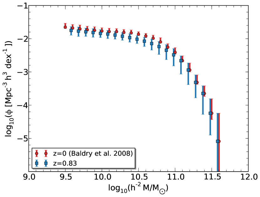
Figure 1: The observed $z{=}0$ (red circles; Baldry et al., 2008) and $z{=}0$.83 (blue squares) stellar mass functions with 68% confidence limits employed as model constraints in this work. For clarity, the $z{=}0.83$ data has been shifted by $-0.02$ dex in stellar mass. The $z{=}0$.83 values and associated uncertainties are a result of homogenising and combining several published Schechter functions (see §4.1 for details).

4.1.2 High redshift

In this paper we also constrain the model using MCMC at redshifts greater than zero. Unfortunately, it is extremely challenging to measure the observed stellar mass function at high redshift. To fully sample both the low and high mass tails of the distribution simultaneously one requires a survey sample of both high depth and large volume. In addition to this, the systematic uncertainties associated with assumptions such as star formation histories become even larger at increasingly higher look-back times, and again, these systematics are often excluded from any quantitative analysis in the literature. It is therefore unsurprising that many published $z{\ga}0.5$ stellar mass functions display significant disagreement, sometimes even at the level of 2$\sigma$.

In order to obtain a single $z{\approx}0.8$ stellar mass function which provides a reasonable estimate of the systematics, we create a weighted average from a number of recently published Schechter function fits in the literature: Drory et al. (2009)($z{=}0.8$–1.0), Ilbert et al. (2010)($z{=}0$.8–1.0), Pozzetti et al. (2007)($z{=}0.7$–9.0). Each was converted from a Chabrier (2003) IMF to a Salpeter (1955) IMF using a constant offset of $+0.24\,\log_{10}(M_{*}/\mathrm{M_{\sun}})$ in stellar mass. All values were also homogenised to $h$=1 and the mass functions cut at the relevant mass completeness limits of each sample. Pozzetti et al. (2007) provides four mass function fits calculated from the VVDS (Visible Imaging Multi-Object Spectrograph; Le Fèvre et al., 2005) survey using two different sample selection criteria and two alternative star formation history models. In total, we therefore employ six observed stellar mass functions covering a redshift range of $z{=}0.7$–1.0.

Our final result was calculated by averaging these homogenised observations to provide a single mass function at a mean redshift of $z{=}0.83$. This was done as follows: All of the utilised mass functions provide $\pm\,1\sigma$ uncertainties on the best fitting Schechter function parameter values. We incorporate these by taking each Schechter function in turn and generating 1000 realisations with parameter values randomly sampled from appropriate probability distributions. Ideally these distributions would account for the covariance which exists between the different fitted parameters, but this information was not provided in the relevant publications. Instead we sampled Gaussian (or skewed Gaussian) distributions centered on the best fit values and with their quoted standard deviations. The mean and $1\sigma$ uncertainties of $\phi$ in each stellar mass bin are then calculated using the random realisations from all six of the observed input functions. To ensure consistency with the $z{=}0$ stellar mass function of Baldry et al. (2008) we demand that $\phi$ and its upper uncertainty is less than or equal to the respective $z{=}0$ values at all stellar masses. Such a restriction is well justified given that the observed total stellar mass density is found to decrease by approximately a factor of a half between $z{=}0$–1 (Drory et al., 2009).

Our final aggregated $z{=}0.83$ stellar mass function is shown in Fig. 1. As a simple first order check of its validity, we confirm that the integrated stellar mass density, over the range of stellar masses present, is $0.64^{+0.21}_{-0.19}$ times that of the $z{=}0$ value. The upper and lower bounds here account for the uncertainty in the mass functions at both redshifts. This shows broad agreement with observational results (e.g. Marchesini et al., 2009). For comparison, Fig. 1 also displays the constraining $z{=}0$ observations of Baldry et al. (2008).

In order to calculate the likelihood of the model stellar mass functions, given the observational data, we use a simple $\chi^{2}$ statistic. For a single stellar mass bin:

$$\mathcal{L}_{\mathrm{SMF}}(\theta)\propto\exp(-0.5\chi^{2}(\theta))=\exp\left(-\frac{1}{2}\frac{(\phi_{\mathrm{obs}}-\phi_{\mathrm{mod}}(\theta))^{2}}{\sigma_{\mathrm{obs}}^{2}+\sigma^{2}_{\mathrm{mod}}(\theta)}\right)\>,$$ (10)

where $\theta$ is the set of model parameters used and $\sigma$ represents the associated uncertainties in each measurement. We estimate $\sigma_{\mathrm{mod,i}}$ using Poisson statistics to be $\sqrt{n_{i}}\,h^{3}\mathrm{Mpc^{-3}dex^{-1}}$, where $n_{i}$ is the number of model galaxies in bin $i$.

We note that a number of previous works which have calibrated semi-analytic models using MCMC techniques have tended to favor the use of the $K$–band luminosity function as their primary constraint instead of the stellar mass function (Henriques et al., 2009; Lu et al., 2012). As the $K$–band is well known to be a good proxy for stellar mass, both quantities provide comparable constraints on the galaxy population. As discussed above, it can be difficult to derive accurate stellar masses for observed galaxies due to the degeneracies and poorly understood systematics of dust attenuation, mass–light ratios and IMFs. Luminosity functions are, however, directly observable and it is for this reason that they have been adopted by previous works. Unfortunately, producing a luminosity function from a semi-analytic model involves many of the same poorly understood physics and systematic uncertainties. Specifically, we must include assumptions about dust attenuation and stellar population synthesis models, in order to convert model stellar masses to luminosities.

As discussed previously, having realistic estimates of the relevant uncertainties is important for our MCMC analysis. Thus, we prefer to implement the stellar mass function as the primary constraint, due to the availability of a number of works which provide a quantitative analysis of some of the uncertainties associated with measuring a stellar mass function at various redshifts (e.g. Baldry et al., 2008; Pozzetti et al., 2007; Marchesini et al., 2009). Although it is true that these uncertainties may still be underestimated, a similar estimate of the systematics associated with a model derived luminosity function is beyond the scope of this paper.

4.2 The Black Hole–Bulge Relation

It is well established that the masses of central super-massive black holes show direct correlations with the properties of their hosts’ bulges (e.g. Magorrian et al., 1998; Häring & Rix, 2004; Sani et al., 2011). This suggests a physical connection between the mass growth of these two components. Given the importance of AGN feedback in shaping the galaxy population, especially for high galaxy masses at $z{<}1$, it is important that our model be able to reproduce this observed relation. This is especially so if we wish to use the model to make any predictions for how black holes of different masses populate different galaxy types.

Similarly to Henriques et al. (2009), we implement the observations of Häring & Rix (2004) as our constraint for the $z{=}0$ black hole–bulge relation. Their sample is comprised of 30 nearby galaxies (the majority of objects being ${\la}42\,h^{-1}\mathrm{Mpc}$ away) with the bulge and black hole masses sourced from a number of different works.

Observationally, it is still unclear whether or not there is a significant evolution in the black hole–bulge relation between $z{=}0$ and $z{=}1$. In general, an evolution is predicted by theory (e.g. Croton, 2006), and is tentatively measured by a number of authors (e.g. McLure et al., 2006; Merloni et al., 2010). Unfortunately, observations of $z{>}0$ black hole–bulge relations are generally hampered by systematic uncertainties which, when included, make the significance of a deviation from the null hypothesis of no evolution much less certain (Schulze & Wisotzki, 2011). For this reason, we choose not to implement a black hole–bulge relation constraint at $z{=}0.83$.

To asses the likelihood of our model fit to the data, we implement the same likelihood calculation as that of Henriques et al. (2009). First, the galaxy sample is segregated into two bins defined by lines perpendicular to the best fit relation of Häring & Rix (2004):

$$\log_{10}(M_{\rm BH})=-0.89(\log_{10}(M_{\rm bulge}/{\rm M_{\sun}})-11)+{\rm offset}$$ (11)

where ${\rm offset{=}[5.39,8.2,12.23]}$. The binomial probability theorem is then used to calculate what the likelihood is of finding the ratio of observed galaxies above and below the Häring & Rix (2004) best fit line in each bin:

$$\mathcal{L}_{\mathrm{BHBR}}=\left\{\begin{array}[]{l l}2I_{p}(k,n-k+1)&\quad Ip\leq 0.5\\ 2(1-I_{p}(k,n-k+1))&\quad Ip>0.5\\ \end{array}\right.\>,$$ (12)

where $k$ is the number of observed galaxies above the best fit line in each bin, $n$ is the total number of galaxies in the bin, and $p(\theta)$ is the fraction of galaxies above the best fit line from the model. $I_{p}(x,y)$ is the regularised incomplete gamma function. As described in Henriques et al. (2009), the reason for using two formulae with conditions is to ensure that any excess of galaxies both above and below the best fit line results in a low likelihood (i.e. both tails of the distribution).

5 Analysis

In this section we present our main analysis. First, we investigate the restrictions placed on the model parameters by the individual observations at $z{=}0$ and $z{=}0.83$. This allows us to test which parameters are most strongly constrained by each observation as well as identify any tensions between these constraints. The findings are then used to guide our interpretation when calibrating the model against all three of our constraints at both redshifts simultaneously (§5.3).

5.1 Redshift zero

5.1.1 The Stellar Mass Function

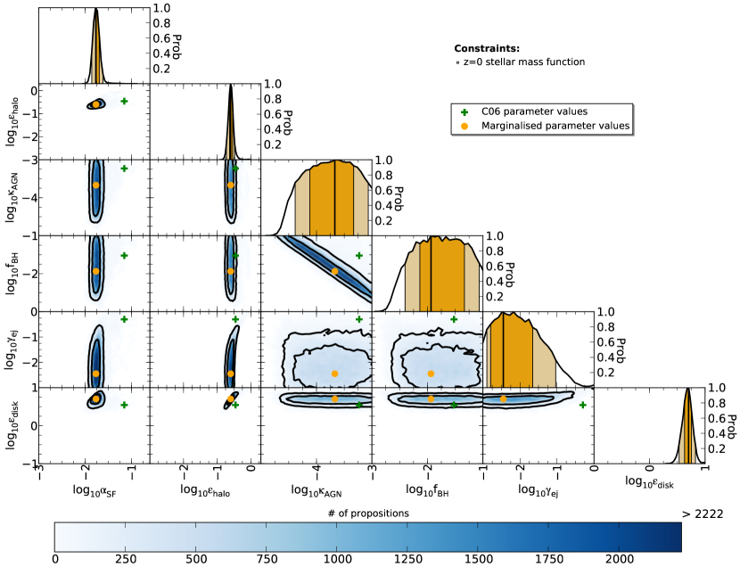
Figure 2: 2-D posterior probability distributions (off-diagonal panels) for all combinations of the six free model parameters when constraining the model against the $z{=}0$ stellar mass function alone. Black lines indicate the 1 and 2-$\sigma$ confidence contours. The limits of each panel indicate the prior ranges. Orange circles show the location of the marginalised best values of each parameter. The histograms in the diagonal panels represent the 1-D marginalised probability distributions, with the 1 and 2$\sigma$ confidence intervals shown by the dark and light shaded regions respectively.

We begin by considering the $z{=}0$ stellar mass function and investigate the restrictions placed on the model parameters by this constraint alone. The histograms on the diagonal panels of Fig. 2 display the 1-dimensional marginalised posterior distributions for each of the six free parameters. The highly peaked, Gaussian-like distributions of the star formation ($\alpha_{\mathrm{SF}}$), supernova halo gas ejection ($\epsilon_{\mathrm{halo}}$), and supernova cold gas reheating ($\epsilon_{\mathrm{disk}}$) efficiencies indicate that these are well constrained by the observed $z{=}0$ stellar mass function alone. Conversely, the wide and relatively flat distributions of the merger driven black hole growth ($f_{\mathrm{BH}}$) and radio mode AGN heating ($\kappa_{\mathrm{AGN}}$) efficiencies, suggest that their precise values are not particularly well constrained. The remaining off-diagonal panels of Fig. 2 show the 2-dimensional posterior probability distributions for all combinations of the six free model parameters (blue shaded regions). The black contours indicate the associated 1 and 2-$\sigma$ confidence intervals.

Although the $z{=}0$ stellar mass function alone does not allow us to say what the precise values of the merger driven black hole growth efficiency ($f_{\mathrm{BH}}$) and radio mode AGN heating efficiency ($\kappa_{\mathrm{AGN}}$) must be, it does place a strong constraint on their ratio. This is indicated by the 2-D posterior distribution of $f_{\mathrm{BH}}$ vs. $\kappa_{\mathrm{AGN}}$ which shows a strong correlation between the allowed values of these two parameters. This is a direct consequence of the degeneracy between central black hole mass (which is dominated by quasar mode growth and thus $f_{\mathrm{BH}}$) and the value of $\kappa_{\mathrm{AGN}}$ in determining the level of radio mode heating (c.f. Eqn. 8). This heating plays a key role in shaping the high mass end of the stellar mass function where supernova feedback becomes ineffective at regulating the availability of cold gas. A similar degeneracy was also noted by Henriques et al. (2009) when constraining their model against the observed K-band luminosity function.

A principal component analysis of the joint posterior suggests that its variance can be understood predominantly through the combination of two equally weighted principal components. The star formation efficiency ($\alpha_{\mathrm{SF}}$) and supernova halo gas ejection efficiency ($\epsilon_{\mathrm{halo}}$) provide almost no contribution to the variance in either component, indicating that both are truly well constrained by the stellar mass function. On the other hand, the value of the ejected gas reincorporation rate parameter ($\gamma_{\mathrm{ej}}$) does contribute significantly to both components. Interestingly, the supernova cold gas reheating efficiency ($\epsilon_{\mathrm{disk}}$) also makes a dominant contribution to one of the principal components, suggesting that, although it appears well constrained in Fig. 2, small variations about the mean can be accommodated by a combination of changes to the remaining parameters controlling black hole growth and AGN radio mode feedback ($f_{\mathrm{BH}}$ and $\kappa_{\mathrm{AGN}}$).

As well as investigating the parameter constraints and degeneracies, we also wish to know what single set of parameters provides us with the best overall reproduction of the relevant observations. The orange points in Fig. 2 indicate the marginalised best parameter values. This is the parameter set around which there was the largest number of accepted propositions in the MCMC chain. These values, along with their 68% confidence limits, are presented in Table 1.

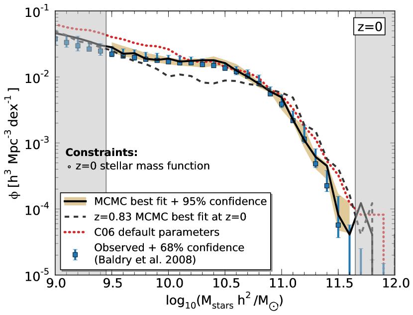
Figure 3: The $z{=}0$ stellar mass function resulting from the best fit parameter values, as determined by constraining the model against the observed $z{=}0$ stellar mass function alone. The solid line with shaded region shows the model result, along with the 95% confidence limits calculated from the posterior distribution. Blue error bars indicate the constraining observations and 68% confidence regions of Baldry et al. (2008). The default Croton et al. (2006) prediction is shown by the red dotted line. Only stellar masses in the unshaded region of the plot were used to constrain the model. The model prediction when using the best fit parameters constrained against the $z{=}0$.83 stellar mass function is also shown for comparison (black dashed line; §5.2).

In Fig. 3 we show the stellar mass function produced by the model using these best fit parameters, as well as the constraining observations of Baldry et al. (2008) and the model prediction using the default Croton et al. (2006) parameters. The orange shaded region encompassing the best fit line indicates the associated 95% confidence limits. These are calculated using all of the mass functions produced during the integration phase of the MCMC chain. When compared to the original Croton et al. (2006) results, the best fit model more accurately reproduces the distribution over the full range of masses - in particular the dip and subsequent rise in galaxy counts that occurs around $10^{10}\>h^{2}\mathrm{M^{-1}_{\sun}}$.

5.1.2 The Black Hole–Bulge Relation

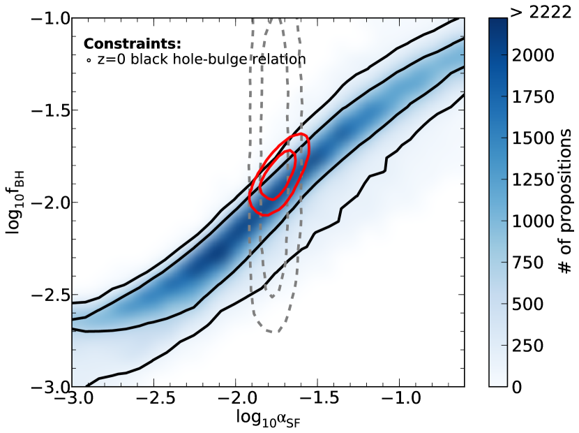
Figure 4: The $f_{\mathrm{BH}}$–$\alpha_{\mathrm{SF}}$ posterior distribution (blue shaded) when constraining the model against the $z{=}0$ black hole–bulge relation alone. Black lines represent the 1 and 2$\sigma$ confidence contours. Grey dashed lines show the equivalent confidence contours found when constraining the model against the $z{=}0$ stellar mass function alone (Fig. 2), whilst red solid lines show the contours found when constraining against the $z{=}0$ stellar mass function and black hole–bulge relation simultaneously.

In order to break the above degeneracy between the merger driven black hole growth and radio mode AGN heating efficiencies ($f_{\mathrm{BH}}$ and $\kappa_{\mathrm{AGN}}$), we require the addition of another constraint which directly ties the properties of the central black holes to those of the galaxies in which they form. Following Henriques et al. (2009), we turn to the observed black hole–bulge mass relation for this purpose. Unlike the stellar mass function, which provides strong constraints in a number of parameter planes, the black hole–bulge relation only constrains the $f_{\mathrm{BH}}$–$\alpha_{\mathrm{SF}}$ (star formation efficiency) plane.

The utility of this particular constraint can be traced to the fact that it provides a relation between the mass of the central black hole and spheroidal component of a galaxy. Bulges can grow in the model via two different mechanisms. The first is through merger events. However, none of the six free model parameters directly influence the strength of this mechanism. The second method of bulge growth is via disk instabilities. We treat this using a modified version of the simple, physically motivated prescription of Mo et al. (1998) whereby, once the surface density of stellar mass in the disk of a galaxy becomes too great, the disk becomes unstable. In this situation, a fraction of the disk stellar mass is transferred to the bulge component in order to restore stability. Hence, bulge growth via this mechanism is regulated by the amount of stars already present in the disk as well as the mass of new stars forming at any given time. These, in turn, are modulated by the efficiency of star formation ($\alpha_{\mathrm{SF}}$). Black holes, on the other hand, gain the majority of their mass via the merger driven quasar mode which is regulated by $f_{\mathrm{BH}}$.

The posterior probability distribution for the black hole–bulge relation constraint alone is shown in Fig. 4. As expected, increasing the efficiency of star formation ($\alpha_{\mathrm{SF}}$), and therefore the growth of bulges through disk instabilities, requires an increase in the efficiency of black hole growth ($f_{\mathrm{BH}}$). Although omitted here for brevity, the constraints provided by this observation on the three parameters which modulate star formation and supernova feedback, are extremely weak. However, in the case of the supernova halo gas ejection efficiency parameter ($\epsilon_{\mathrm{halo}}$), the marginalised posterior distribution only overlaps with those of the stellar mass function constraint to within $2\sigma$. In other words, there is a slight tension between the parameter sets favoured by the black hole–bulge relation and stellar mass function.

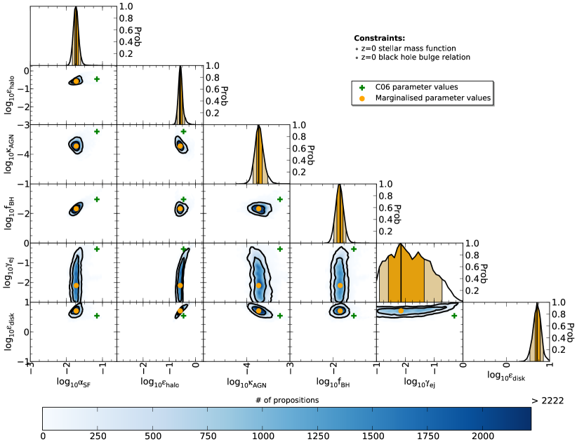
Figure 5: 2-D posterior probability distributions (off-diagonal panels) for all combinations of the six free model parameters when constraining the model against the $z{=}0$ stellar mass function and black hole–bulge relation simultaneously. Black lines indicate the 1 and 2-$\sigma$ confidence contours. The limits of each panel indicate the prior ranges. Orange circles show the location of the marginalised best values of each parameter. The histograms in the diagonal panels represent the 1-D marginalised probability distributions, with the 1 and 2-$\sigma$ confidence intervals indicated by the dark and light shaded regions respectively. This figure can be directly compared with Fig. 2.

In Fig. 5 we show the marginalised posterior distributions for the six model parameters when constrained against both the $z{=}0$ stellar mass function and $z{=}0$ black hole–bulge relation simultaneously. The joint probability of a particular model parameter set is determined by calculating the likelihoods for each constraint individually, as outlined above, and then combining these with equal weights using standard probability theory:

$$\mathcal{L}(\theta)=\mathcal{L}_{\mathrm{SMF}}(\theta)\cdot\mathcal{L}_{\mathrm{BHBR}}(\theta)$$ (13)

As expected, the distributions look similar to those of Fig. 2, with the exception that we now also tightly constrain the values of the merger driven black hole growth and radio mode AGN feedback efficiencies ($f_{\mathrm{BH}}$ and $\kappa_{\mathrm{AGN}}$) through the addition of the information contained in Fig. 4. Unfortunately, we are still only able to provide an upper limit on the value of the re-incorporation efficiency parameter, $\gamma_{\mathrm{ej}}$. However, this does tell us that the model prefers re-incorporation of ejected gas to occur on a timescale longer than approximately 10 halo dynamical times (roughly equivalent to the Hubble time).

A principal component analysis indicates that the addition of the black hole–bulge relation constraint has reduced the number of principal components from two to one. This confirms that we have successfully reduced the freedom of the parameter values with respect to one another. Again we find that star formation efficiency, $\alpha_{\mathrm{SF}}$, is fully constrained. However, we now find that supernova cold gas reheating efficiency, $\epsilon_{\mathrm{disk}}$, also contributes practically no information on the variance of the joint posterior distribution. This is due to the fact that we have now restricted the allowed values of the black hole growth and radio mode AGN heating efficiencies ($f_{\mathrm{BH}}$ and $\kappa_{\mathrm{AGN}}$), thus preventing them from compensating for any small shift to $\epsilon_{\mathrm{disk}}$, as was allowed when constraining against the $z{=}0$ stellar mass function alone.

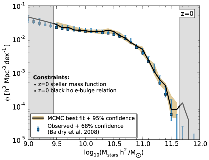
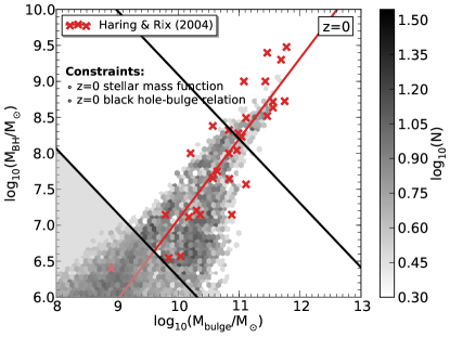
Figure 6: The $z{=}0$ model stellar mass function (left) and black hole–bulge relation (right) obtained using the marginalised best parameter values found when constraining against both the $z{=}0$ stellar mass function and black hole–bulge relation simultaneously. For the stellar mass function, the solid line with shaded region shows the model result along with the 95% confidence region calculated from the posterior distribution. Blue error bars show the constraining observations of Baldry et al. (2008). In the right hand panel, the model galaxies are indicated by the shaded grey hexbins, while the observational constraint of Häring & Rix (2004) is shown as the red crosses along with the published best fit line.

In Fig. 6 we show the $z{=}0$ stellar mass function and black hole–bulge relation obtained using the marginalised best parameters. These parameter values form our fiducial $z{=}0$ set and are listed in Table 1.

A comparison with Fig. 3 indicates that our reproduction of the observed stellar mass function remains excellent. However, we note that the likelihood of the black hole–bulge relation is only 0.2 when including the stellar mass function constraint. This is caused by a slight tension between the preferred parameter values of these two constraining observations. A similar result was found by Henriques et al. (2009) when calibrating their model against the $K$-band luminosity function and black hole–bulge relation.

Despite this drop in likelihood, statistical agreement within 2$\sigma$ is still achieved and the resulting black hole–bulge relation remains cosmetically acceptable. Finally, we note that a great deal of observational uncertainty remains in the precise normalisation and slope of the black hole–bulge relation. It is therefore possible that future black hole–bulge relation measurements will result in a relation that is more easily reconciled with the stellar mass function in our model.

5.2 High redshift

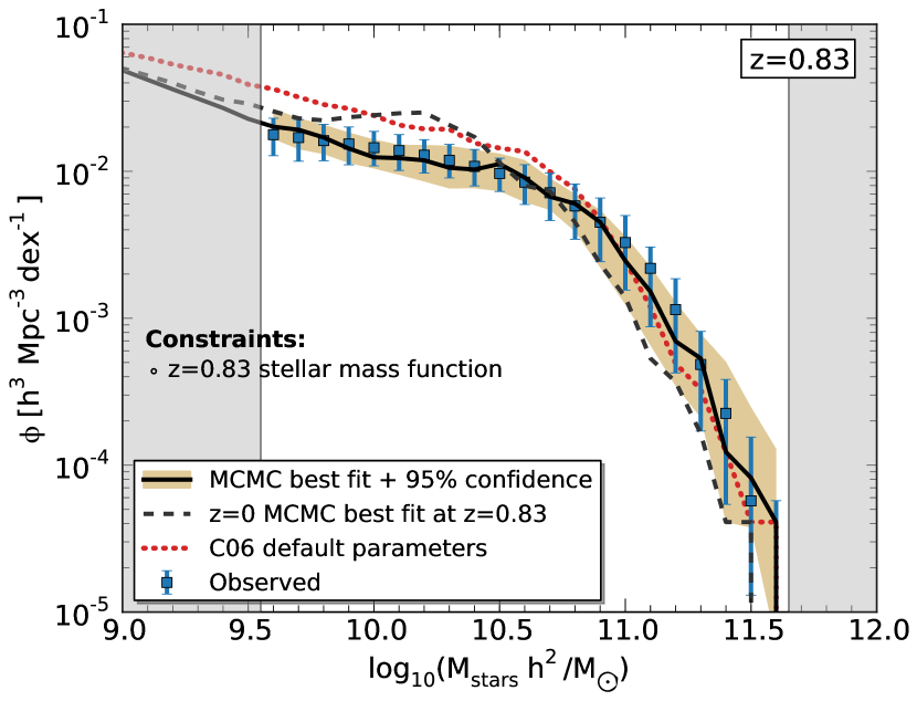
Figure 7: The resulting $z{=}0.83$ stellar mass function and 95% confidence regions (black line and shaded region) produced by constraining the model against the observed $z{=}0.83$ stellar mass function alone. The constraining observations and 1$\sigma$ uncertainties are shown as blue error bars (c.f. §4.1.2). Also shown for comparison are the $z{=}0.83$ stellar mass functions produced by the default Croton et al. (2006) (red dotted line) and $z{=}0$ fiducial (black dashed line) parameter values.

In the last section we investigated the constraining power of the $z{=}0$ stellar mass function and black hole–bulge relation. These observational quantities allowed us to place strong restrictions on the values of all but one of the free model parameters. In this section we investigate the resulting $z{>}0$ model predictions and also implement our $z{=}0.83$ stellar mass function constraint on its own (§4.1) in order to test the restrictions it imposes on the model parameters.

In Fig. 7 we show the prediction of the default Croton et al. (2006) model parameter values (red dotted line), compared against the observed stellar mass function at $z{=}0.83$ (blue squares; see §4.1 for details). Similarly to the redshift zero case, the default model over-predicts the number of galaxies at low masses. However, it now also predicts a steeper slope to the high mass end than is observed.

Also shown in Fig. 7 is the result obtained using the fiducial $z{=}0$ parameters of the previous section. This model predicts an unrealistic build up of galaxies around $\log_{10}(M\,[h^{2}/\mathrm{M_{\sun}}]){=}10.25$ which constitutes the population that will later evolve to fill the high mass end of the distribution at $z{=}0$. This over-density is a direct result of under-efficient supernova feedback, allowing lower mass galaxies to hold on to too much of their cold gas which is subsequently converted into stellar mass. Overall, the fiducial $z{=}0$ parameters appear to do a worse job of reproducing the $z{=}0.83$ observations than the original Croton et al. (2006) values.

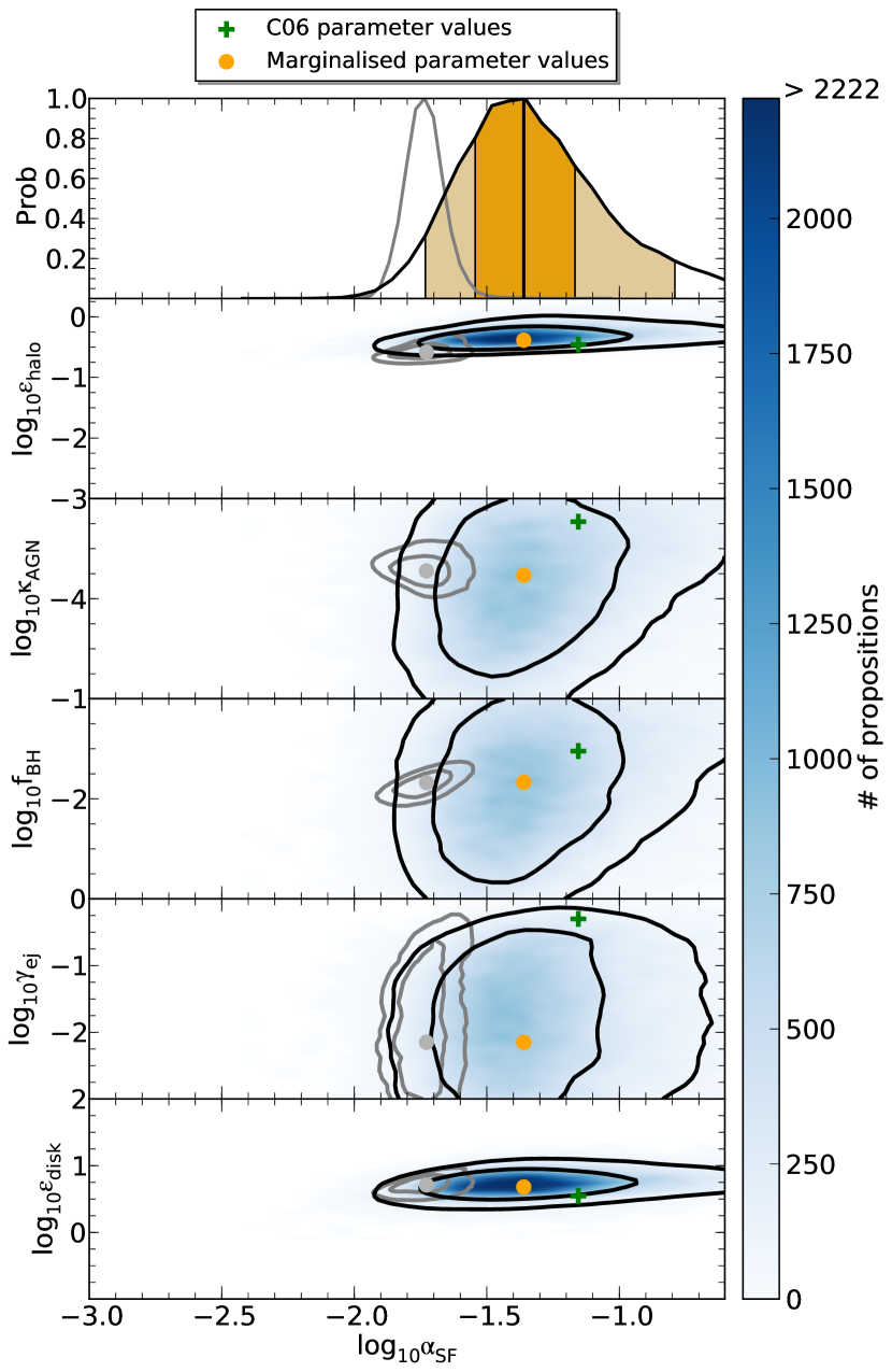
Figure 8: 2-D posterior probability distributions for the star formation efficiency, $\alpha_{\mathrm{SF}}$, against the five other free model parameters when constraining the model against the $z{=}0.83$ stellar mass function alone. The limits of each panel are equivalent to the MCMC prior ranges. Orange circles indicate the location of the marginalised best values of each parameter. Black lines represent the 1 and 2$\sigma$ confidence contours with grey lines indicating the equivalent results from Fig. 5. The histogram in the top panel displays the 1-D marginalised probability distribution for $\alpha_{\mathrm{SF}}$, with the 1 and 2$\sigma$ confidence intervals shown by the dark and light shaded regions respectively.

The solid black line and shaded region of Fig. 7 indicate the best fit mass function and associated 95% confidence regions found by constraining against the observed $z{=}0.83$ stellar mass function alone. An excellent agreement can be seen across all masses. The marginalised best parameter values and 68% uncertainties are listed in Table 1. A subset of the posterior probability distributions are presented in Fig. 8. For comparison, the equivalent 1 and 2$\sigma$ confidence regions of the $z{=}0$ stellar mass function+black hole–bulge relation constraint from Fig. 5 are also indicated with grey contour lines.

As was the case when constraining the model against the $z{=}0$ stellar mass function alone (§5.1.1), there is little restriction on the values of black hole growth and radio mode AGN feedback efficiencies ($f_{\mathrm{BH}}$ an $\kappa_{\mathrm{AGN}}$). This is due to the fact that we have no black hole–bulge relation constraint to break the degeneracy between these two parameters. The star formation efficiency ($\alpha_{\mathrm{SF}}$) confidence region is also significantly larger at $z{=}0$.83 compared to $z{=}0$. This is primarily a reflection of the larger observational uncertainties across all stellar masses at this redshift. Interestingly, we also find that the most likely value of the supernova cold gas reheating parameter, $\epsilon_{\mathrm{disk}}$, shows little evolution between redshifts, despite the need to increase the upper prior limit on this parameter to account for a slightly extended probability tail extending past our original upper limit of $\epsilon_{\mathrm{disk}}$=10.

The parameters controlling star formation and supernova halo gas ejection efficiencies ($\alpha_{\mathrm{SF}}$ and $\epsilon_{\mathrm{halo}}$) display the largest differences in posterior distributions with respect to $z{=}0$. In fact, a principal component analysis suggests that the only parameter which is truly well constrained by the $z{=}0.83$ stellar mass function is $\alpha_{\mathrm{SF}}$. Its value is approximately 2.5 times higher than was the case at $z{=}0$ which is driven by the need to form high mass galaxies more rapidly in order to achieve a better match to the massive end of the observed stellar mass function. However, a side effect is the further build up of galaxies at intermediate masses ($\log_{10}(M\,[h^{2}/\mathrm{M_{\sun}}]){=}10.0{-}10.5$) which must then be alleviated by increasing the strength of the supernova cold gas ejection efficiency, $\epsilon_{\mathrm{halo}}$.

From Eqn. 5, we see that the amount of gas ejected from the dark matter halo entirely by supernova feedback equals zero for $V_{\mathrm{vir}}{>}V_{\mathrm{vir}}^{\mathrm{cutoff}}{=}V_{\mathrm{SN}}(\epsilon_{\mathrm{halo}}/\epsilon_{\mathrm{disk}})^{1/2}$. Hence by increasing $\epsilon_{\mathrm{halo}}$ (the halo hot gas ejection efficiency), we increase the characteristic halo mass at which supernova feedback becomes ineffective at ejecting gas from the system. The net result is a reduction of star formation in more massive galaxies (which preferentially populate dark matter halos with higher masses, and hence higher virial velocities) due to a reduced availability of hot gas which can then cool to fuel star formation.

Given that $V_{\mathrm{vir}}^{\mathrm{cutoff}}$ depends on the ratio of the supernova ejection and reheating parameters ($\epsilon_{\mathrm{halo}}$ and $\epsilon_{\mathrm{disk}}$), why does the $z{=}0$.83 stellar mass function preferentially modify $\epsilon_{\mathrm{halo}}$ from its $z{=}0$ fiducial value instead of $\epsilon_{\mathrm{disk}}$? Again from Eqn. 5, we see that a change in $\epsilon_{\mathrm{disk}}$ results in a proportional change to the ejected mass. However, this is independent of the host halo properties. On the other hand, modifying $\epsilon_{\mathrm{halo}}$ results in a change to the ejected mass with a magnitude that is inversely proportional to $V_{\mathrm{vir}}^{2}$. Hence increasing $\epsilon_{\mathrm{halo}}$ results in both an increase in the value of $V_{\mathrm{vir}}^{\mathrm{cutoff}}$, as well as preventing the build-up of excess star forming galaxies just above this halo velocity where radio mode black hole feedback is still inefficient.

5.3 Combined redshifts

Having presented the results of constraining the model to match observations at $z{=}0$ and 0.83 individually, we now investigate if it is possible to achieve a satisfactory result at both redshifts simultaneously. As shown in Fig. 8, there is some tension between the marginalised posterior distributions at each redshift. However, it is possible that a parameter configuration may exist which, although not achieving the best possible reproduction at either redshift, will still provide a satisfactory combined result.

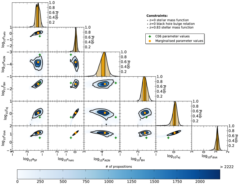
Figure 9: 2-D posterior probability distributions (off-diagonal panels) for all combinations of the six free model parameters when constraining against the $z{=}0$ and $z{=}0$.83 stellar mass functions, and the $z{=}0$ black hole–bulge relation, all simultaneously. Black lines indicate the 1 and 2-$\sigma$ confidence contours. The limits of each panel indicate our prior ranges. Orange circles show the location of the marginalised best values of each parameter, while red diamonds indicate the values from the single parameter set which produced the best reproduction of the observations (maximum likelihood parameters). The histograms in the diagonal panels represent the 1-D marginalised probability distributions, with the 1 and 2-$\sigma$ confidence intervals indicated by the dark and light shaded regions respectively. The 1-D maximum likelihood distributions are also shown for comparison (red dashed lines). This figure can be directly compared with Figs. 2 and 5.

Fig. 9 shows the 1 and 2-D posterior distributions for the model when constrained simultaneously against the $z{=}0$ stellar mass function and black hole–bulge relation, as well as the $z{=}0.83$ stellar mass function. The 1-D histograms indicate that this constraint combination places strong restrictions on all of the free model parameters, including the ejected gas reincorporation rate parameter, $\gamma_{\mathrm{ej}}$. For all previously investigated constraint combinations, the value of $\gamma_{\mathrm{ej}}$ has made little impact on the ability of the model to reproduce the relevant observations. This has been true for values spanning several orders of magnitude. However, when constraining the model to reproduce two redshifts simultaneously, gas reincorporation rate plays a key role.

As discussed in §5.2, the individual redshift constraints provide strong, but irreconcilable, restrictions on the value of the star formation efficiency, $\alpha_{\mathrm{SF}}$. When these constraints are combined, the model is therefore forced to pick one of the preferred $\alpha_{\mathrm{SF}}$ values and use the freedom in the other parameters, including $\gamma_{\mathrm{ej}}$, to maximise the joint likelihood.

The main effect of altering the ejected gas reincorporation efficiency, $\gamma_{\mathrm{ej}}$, occurs at the low mass end of the stellar mass function. It’s only here that supernova feedback is efficient at expelling gas and galaxies have a significant amount of material in their ejected reservoirs. In addition, in our model the ejected mass reservoirs of in-falling satellite galaxies are immediately incorporated into the hot halo components of their more massive parents and hence no extra material is added to the ejected component of these larger systems. By increasing the value of $\gamma_{\mathrm{ej}}$ the timescale over which expelled gas makes its way back into the heating/cooling cycle is decreased. This results in more cold gas being available for forming stars in the lowest mass galaxies, with the net effect being a raising of the low mass end of the stellar mass function.

As shown in Fig. 7, the fiducial $z{=}0$ parameter set already produces a stellar mass function at $z{=}0.83$ which is overabundant in low mass galaxies. In order for $\gamma_{\mathrm{ej}}$ to help to alleviate this, its value needs to be reduced, thus reincorporating less ejected gas into lower mass systems. Unfortunately however, the marginalised best value of $\gamma_{\mathrm{ej}}$ using the $z{=}0$ constraints is already extremely low ($1.7{\times}10^{-3}$) and reducing it even further has a negligible effect. The model is therefore unable to utilise this parameter to maximise the joint-redshift likelihood when using the fiducial $z{=}0$ star formation efficiency. Fortunately however, $\gamma_{\mathrm{ej}}$ can be used to maximise the likelihood achieved with the $z{=}0.83$ preferred parameters.

Compared to the $z{=}0$ case, the $z{=}0.83$ marginalised best parameters have a higher star formation efficiency, $\alpha_{\mathrm{SF}}$, resulting in a more rapid transition of galaxies from low to high masses. As shown in Fig. 3, the effect on the stellar mass function at $z{=}0$ is an over-abundance at high stellar masses and a corresponding under-abundance at low masses. Increasing the low value of the gas reincorporation rate parameter ($\gamma_{\mathrm{ej}}$) can have a significant effect here by increasing the number of galaxies below the knee of the mass function. By also increasing the values of the supernova feedback gas reheating and ejection parameters ($\epsilon_{\mathrm{disk}}$ and $\epsilon_{\mathrm{halo}}$) the model can achieve the correct overall shape whilst moving the position of the knee by only a small amount. This allows a better reproduction of the $z{=}0$ mass function to be achieved.

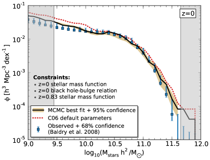
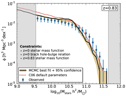
Figure 10: The $z{=}0$ (left) and $z{=}0.83$ (right) model stellar mass functions obtained using the highest likelihood model parameters when constraining against the $z{=}0$ and $z{=}0.83$ stellar mass functions, and the $z{=}0$ black hole–bulge relation, simultaneously. The solid line with shaded region shows the model result along with the 95% confidence region calculated from the posterior distributions. Blue error bars show the relevant constraining observations.

The marginalised best values and their uncertainties are presented in Table 1. Fig. 10 displays the resulting $z{=}0$ and 0.83 stellar mass functions. Even though the star formation efficiency parameter is close to the preferred $z{=}0.83$ value, the changes made to the other parameters have resulted in a visually poorer reproduction of $z{=}0.83$ mass function. However, a reduced $\chi^{2}$ of 1.28 (with 14 degrees of freedom) indicates that the fit of the highest likelihood line is still statistically acceptable. In order to achieve this level of agreement at both redshifts simultaneously, we note that we have been required to push the parameters associated with supernova feedback and reincorporation ($\epsilon_{\mathrm{disk}}$, $\epsilon_{\mathrm{halo}}$ and $\gamma_{\mathrm{ej}}$) to values that are perhaps unrealistic. We discuss the interpretation and possible physical implications of this outcome in the next section.

Finally we note that we have increased the lower limit on the reincorporation efficiency ($\gamma_{\mathrm{ej}}$) prior to 0.1 when applying our joint redshift constraints. In testing, we allowed this parameter to go as low as $10^{-3}$, however, we found that this introduced a large peak in the marginalised posterior distributions, corresponding to the alternative, but lower probability, $z{=}0$ preferred star formation efficiency ($\alpha_{\mathrm{SF}}$). As discussed above, in order to maximise the likelihood achieved using this $\alpha_{\mathrm{SF}}$ value, the reincorporation efficiency must be lowered as much as possible. However, all values of $\gamma_{\mathrm{ej}}{\la}0.1$ produce approximately identical joint likelihoods as any sufficiently small value results in almost no mass of ejected material being reincorporated in to low mass halos. When these low mass halos grow sufficiently, they will eventually reincorporate the material. However, they will also have set up a hydro-static hot halo, meaning the effect of recapturing this mass on the central galaxy will be minimal.

When we allowed the reincorporation efficiency to go to lower values the MCMC chain spent a large number of successful proposals mapping out the extensive volume provided by this flat low likelihood feature. Each of these propositions contributed to a marginalised peak coinciding with the lower likelihood $z{=}0$ preferred star formation efficiency. This feature of the posterior distribution highlights the importance of selecting suitable priors which encompass the full range of physically plausible parameter values, but which do not include large areas of parameter space which are indistinct from each other due to the details of the model.

If we were to have allowed values of $\gamma_{\mathrm{ej}}{\la}0.1$ in our presented analysis, we would have unfairly biased our posterior distributions towards a region of lower likelihood. It is important to note however, that given a suitably long chain, the MCMC would eventually still have converged to provide us with the same posterior distribution peaks as presented in Fig. 9. Our poor choice of lower prior for $\gamma_{\mathrm{ej}}$ would simply have meant that such a convergence would have required an unfeasibly long chain.

6 Discussion

6.1 Interpreting the joint redshift constraint results

The fiducial parameter values for our joint redshift constraints (c.f. table 1) provide us with a valuable insight into exactly where the tensions lie within the model when trying to successfully reproduce the late time growth of stellar mass in the Universe. The parameters associated with supernova feedback have been pushed to their limits, and possibly to unrealistic values. Using our MCMC analysis of the model when constrained against each redshift individually allows us to understand the cause of this as follows:

• The values of all of the parameters are driven by the need to put the high mass end of the stellar mass function in place as early as possible. This is illustrated in Fig. 7 where we see that the high redshift stellar mass function produced by the $z{=}0$ fiducial parameter values (dashed line) under predicts the number density of high mass galaxies. In order to alleviate this discrepancy and provide the best possible match to the observations at $z$=0.83 alone, a relatively high star formation efficiency is required (see Fig. 8).

• Unfortunately, as shown in Fig. 3, this high star formation efficiency causes an under-prediction of the number of low mass galaxies at $z{=}0$, due to their rapid growth. In order to counteract this and to provide the best possible result at both redshifts simultaneously, the preferred re-incorporation rate of ejected material ($\gamma_{\mathrm{ej}}$) must be increased. This efficiently increases the number density of galaxies with stellar masses below the knee of the mass function whilst leaving the high mass distribution unchanged. Although not implausible, it is worth noting that such a high value of $\gamma_{\mathrm{ej}}$ requires the presence of some mechanism to rapidly return ejected material into the heating/cooling cycle over timescales close to, or less than, the dynamical time of the host dark matter halo.

• However, the rise in the number of very low stellar mass galaxies that results from such a high gas re-incorporation efficiency is extremely large and leads to an overestimation of their number density at both redshifts. To compensate, the preferred supernova halo gas ejection efficiency ($\epsilon_{\mathrm{halo}}$) is forced to values greater than one, implying that either the mean kinetic energy of supernova explosions per unit mass is too low, or that some other physical mechanism exists to enhance the deposition of this energy into the ISM.

• Increasing the value of the supernova ejection efficiency to such high values allows for the efficient regulation of star formation in larger and larger systems, thus pushing the knee of the $z{=}0$ stellar mass function to higher masses. In order to return the knee to its correct position the model is forced to equivalently increase the supernova feedback mass loading factor ($\epsilon_{\mathrm{disk}}$) to ${\approx}14$. Unfortunately, such a high mass loading factor is difficult to reconcile with current observational estimates (e.g. Martin, 1999; Rupke et al., 2002; Martin, 2006) and may suggest the need for an additional halo mass dependence for this parameter (e.g. Oppenheimer & Davé, 2006; Hopkins et al., 2012).

The high values preferred by these parameters suggests that the model prescriptions for supernova feedback, and possibly gas re-incorporation, are insufficient. Similar assertions have been made by other works, most commonly based upon calibrating semi-analytic models to reproduce the $z{=}0$ stellar mass or luminosity functions and then investigating the $z{>}0$ predictions (e.g. Guo et al., 2011; Lu et al., 2012). However, we confirm this finding for the first time through explicitly attempting to match the observed stellar mass functions at two redshifts simultaneously. This allows us to exclude the possibility that a physically acceptable parameter combination exists within the framework of our current physical prescriptions.

6.2 Implications

In Fig. 10 we show the highest likelihood stellar mass functions produced by the model when simultaneously constrained against the observed $z{=}0$ and 0.83 stellar mass functions and the $z{=}0$ black hole–bulge relation. Although we do manage to achieve statistically reasonable fits to the stellar mass function at both epochs, there are some clear tensions at high redshift. We now discuss the possible implications for our semi-analytic model as well as for the growth of stellar mass in the Universe.

Despite large observational uncertainties associated with measuring the number density of the most massive galaxies at $z{\gg}0$, the phenomenon of galaxy ‘downsizing’, whereby the most massive galaxies in the Universe are in place at early times, is well established (Heavens et al., 2004; Neistein et al., 2006). Our results extend those of previous works in suggesting that current galaxy formation models built upon the hierarchical growth of structure find it difficult to reproduce the quantitative details of this phenomenon (e.g. De Lucia et al., 2006; Kitzbichler & White, 2007; Guo et al., 2011; Zehavi et al., 2012). In particular, a comparison of the stellar mass functions produced when constraining against each redshift individually demonstrates that the model struggles to successfully put the highest mass galaxies in place early on (black dashed line of Fig. 7) without also under-predicting the number of low mass galaxies at $z{=}0$ and equivalently over-predicting the number density of the most massive galaxies (black dashed line of Fig. 3).

It is possible that the model’s under-prediction at high masses may be partially alleviated by convolving the $z{=}0.83$ model mass function with a normal distribution of a suitable width in order to account for systematic uncertainties in the observed stellar masses (Kitzbichler & White, 2007; Guo et al., 2011). We do not carry out such a procedure here, as at least some fraction of this uncertainty should be included in our constraining observations and we do not wish to add a further add-hoc correction without justification. However, it may prove impossible for the model to self-consistently reproduce the observed stellar mass function at multiple redshifts without including these additional observational uncertainties (Moster et al., 2012).

In our model, star formation, supernova feedback and gas re-incorporation are assumed to proceed with a constant efficiency as a function of halo mass across the full age of the Universe. However, our findings could be interpreted as suggesting the need to incorporate an explicit time dependence to these efficiencies; in particular to provide a preferential increase to the rate of stellar mass growth in massive halos in the early Universe. This would help establish the high mass end of the stellar mass function early on without over-producing the number of lower mass galaxies at late times.

Unfortunately, adding further layers of parametrisation to current processes, such as an explicit time dependence, makes the interpretation of model results increasingly difficult. This is especially so when attempting to uncover the relative importance of physical processes that shape the evolution of different galaxy populations. To combat this, it is important to ensure that all new additions to a semi-analytic model have a strong physical motivation.

Having said that, modifications to the rate of growth of stellar mass in the early Universe is supported by other studies. In particular, it has been suggested that the star formation efficiency of galaxies must peak at earlier times for more massive galaxies (e.g. Moster et al., 2012). This could possibly represent a number of physical processes such as a metallicity dependent star formation efficiency (Krumholz & Dekel, 2012) or a rapid phase of stellar mass growth due to high redshift cold flows (Dekel et al., 2009). Alternatively, the apparent need to incorporate an explicit time dependence to the star formation and feedback efficiencies could signify an overestimation of the merger timescales in the model at early times (Weinmann et al., 2011). Also, we note that star formation proceeds in our model following a simple gas surface density threshold argument. It may be the case that we are over predicting the size of the most massive galaxies at early redshift and therefore under-predicting the level of star formation in these objects. We do not specifically track the build up of angular momentum in our simulated galaxies, instead relying on the spin of the parent dark matter halo as being a good proxy. It is unlikely that this assumption is valid at high redshift (e.g. Dutton & van den Bosch, 2009; Kimm et al., 2011; Brook et al., 2011) and, even if it were, the low time resolution of our input simulation coupled with the low number of particles in halos at these times might mean that the halo spin values are systematically unreliable here.

Rather than suggesting the need for a time dependent star formation efficiency, an additional interpretation of our findings could be the need to include an intra-cluster light component (ICL) in the model (Gallagher & Ostriker, 1972; Purcell et al., 2007; Guo et al., 2011). Sub-halo abundance matching studies have suggested that mergers involving massive galaxies may result in significant fractions (${\ga}80\%$) of the in-falling satellite mass being deposited in to this diffuse component rather than ending up in the central galaxy (Conroy et al., 2007; Behroozi et al., 2012). Since the majority of late time growth of the most massive galaxies is heavily dominated by mergers, the inclusion of such a stellar mass reservoir may allow the effective suppression of the growth of these massive objects, reducing the need to push the supernova feedback parameters to such extreme values.

Finally, the majority of modern galaxy formation models are now able to reproduce many of the most important observational quantities of the $z{=}0$ Universe. Any changes to the underlying cosmology or input merger tree construction can typically be accounted for by varying the free model parameters. However, achieving the correct time evolution of the full galaxy population is a more difficult task and makes us far more dependant on the details of dark matter structure growth. If this growth does not correctly match the real Universe then this is something that the models will try to counteract, possibly leading us to conclusions about the baryonic physics which could be incorrect. To fully assess the level to which missing or poorly understood baryonic physics are responsible for discrepancies from observed galaxy evolution, a detailed analysis of the effects of cosmology, dark matter halo finding, and merger tree construction on the output of a single galaxy formation model is needed.

7 Conclusions

In this work we investigate the ability of the Croton et al. (2006) semi-analytic galaxy formation model to reproduce the late time evolution of the growth of galaxies from $z{\approx}0.8$ to the present day. In particular we focus on matching the $z{=}0$ and $z{=}0.83$ stellar mass functions as well as the $z{=}0$ black hole–bulge relation. To achieve this we utilise Monte-Carlo Markov Chain techniques, allowing us to both statistically calibrate the model against the relevant observations and to investigate the degeneracies and tensions between different free parameters.

Our main results can be summarised as follows:

• The Croton et al. (2006) model is able to provide a good agreement with the stellar mass function and black hole–bulge relation at $z{=}0$ (§5.1; Figs. 2, 3). However, when attempting to match both simultaneously there are some minor tensions between the favoured parameter values (§5.1; Figs. 4, 6).

• The model is also able to independently provide a good agreement with the observed stellar mass function at $z{=}0$.83. In order to achieve this, a higher star formation efficiency is necessary than was preferred to match the $z{=}0$ constraints. This is to ensure that the massive end of the stellar mass function is entirely in place by this early time, as required by our constraining observations (§5.2; Figs. 7, 8).

• When attempting to reproduce the observations at both redshifts simultaneously, a number of tensions in the model’s physical prescriptions are highlighted. In particular, the struggle to reconcile the high star formation efficiency required to reproduce the high mass end of the stellar mass function at $z{=}0.83$ with the observed increase in normalisation of the low mass end at $z{=}0$ (§5.3; Fig. 10).

• Our attempts to model the evolution of galaxies at $z{\la}0.8$ suggest that the supernova feedback prescriptions of the model may be incomplete, possibly requiring the addition of extra processes that preferentially enhance star formation in the most massive galaxies at $z{>}1$ (§6).

This is the first time that a full semi-analytic model, based on the input of N-body dark matter merger trees, has been statistically calibrated to try and reproduce a small focussed set of observations at multiple redshifts simultaneously. Only by carrying out this procedure, and fully exploring the available parameter space of our particular model, are we able to conclusively demonstrate that the model struggles to match the late time growth of the galaxy stellar mass function. Our analysis also provides us with important insights as to what changes may be necessary to alleviate these tensions. Having said that, despite requiring somewhat unlikely parameter values, we do achieve a statistically reasonable fit to the observations at both redshifts simultaneously. For the purpose of producing mock galaxy catalogues at $z\la 0.8$, this best fit model is perfectly adequate.

For this work, we have only considered the stellar mass function and black hole–bulge relation. However, it is likely that the addition of extra observational constraints will further help to isolate the parts of the model which require particular attention. For example, the gas mass–metallicity relation (Tremonti et al., 2004) is particularly sensitive to the re-incorporation efficiency due to its ability to regulate the dilution of a galaxy’s gas component with low metallicity material ejected at early times. In future work we will extend our analysis to redshifts greater than one and investigate the constraints provided by other quantities such as the mass–metallicity relation as well as the baryonic Tully-Fisher relation, galaxy colour distribution and stellar mass density evolution.

Finally, we also stress that our results and conclusions are sensitive to the magnitude of the uncertainties associated with our observational constraints. Although we have endeavoured to ensure their accuracy, it is likely that they may still be underestimated. For example, the high mass end of $z{\gg}0$ stellar mass functions are heavily susceptible to cosmic variance effects due to the deep observations required to simultaneously resolve galaxies at lower mass scales (typically done in smaller fields). Some works have also suggested systematic uncertainties of 0.3 dex or more when estimating stellar masses via broad-band photometry (Conroy et al., 2009). Furthermore, the magnitude of many of these uncertainties increases significantly with redshift, and can result in errors of up to 0.8 dex around the knee of the measured stellar mass functions at $z=1.3{-}2$ (Marchesini et al., 2009). More detailed comparisons between state-of-the-art semi-analytic models and high redshift observations will therefore require us to greatly improve our measurements at these redshifts.

References

- Baldry et al. (2004) Baldry I. K., Glazebrook K., Brinkmann J., Ivezić Ž., Lupton R. H., Nichol R. C., Szalay A. S., 2004, ApJ, 600, 681
- Baldry et al. (2008) Baldry I. K., Glazebrook K., Driver S. P., 2008, MNRAS, 388, 945
- Behroozi et al. (2012) Behroozi P. S., Wechsler R. H., Conroy C., 2012, arXiv:1207.6105
- Benson (2012) Benson A. J., 2012, New A, 17, 175
- Benson & Bower (2010) Benson A. J., Bower R., 2010, MNRAS, 405, 1573
- Blanton et al. (2005) Blanton M. R. et al., 2005, AJ, 129, 2562
- Bower et al. (2006) Bower R. G., Benson A. J., Malbon R., Helly J. C., Frenk C. S., Baugh C. M., Cole S., Lacey C. G., 2006, MNRAS, 370, 645
- Bower et al. (2010) Bower R. G., Vernon I., Goldstein M., Benson A. J., Lacey C. G., Baugh C. M., Cole S., Frenk C. S., 2010, MNRAS, 407, 2017
- Brook et al. (2011) Brook C. B. et al., 2011, MNRAS, 415, 1051
- Chabrier (2003) Chabrier G., 2003, ApJ, 586, L133
- Cole et al. (2001) Cole S. et al., 2001, MNRAS, 326, 255
- Conroy et al. (2009) Conroy C., Gunn J. E., White M., 2009, ApJ, 699, 486
- Conroy et al. (2007) Conroy C., Wechsler R. H., Kravtsov A. V., 2007, ApJ, 668, 826
- Croton (2006) Croton D. J., 2006, MNRAS, 369, 1808
- Croton et al. (2006) Croton D. J. et al., 2006, MNRAS, 365, 11
- De Lucia & Blaizot (2007) De Lucia G., Blaizot J., 2007, MNRAS, 375, 2
- De Lucia et al. (2006) De Lucia G., Springel V., White S. D. M., Croton D., Kauffmann G., 2006, MNRAS, 366, 499
- Dekel et al. (2009) Dekel A., Sari R., Ceverino D., 2009, ApJ, 703, 785
- Drory et al. (2009) Drory N. et al., 2009, ApJ, 707, 1595
- Dutton & van den Bosch (2009) Dutton A. A., van den Bosch F. C., 2009, MNRAS, 396, 141
- Gallagher & Ostriker (1972) Gallagher, III J. S., Ostriker J. P., 1972, AJ, 77, 288
- Gelman & Rubin (1992) Gelman A., Rubin D. B., 1992, Statistical Science, 7
- Guo et al. (2011) Guo Q. et al., 2011, MNRAS, 413, 101
- Häring & Rix (2004) Häring N., Rix H.-W., 2004, ApJ, 604, L89
- Hastings (1970) Hastings W. K., 1970, Biometrika, 57, 97
- Hatton et al. (2003) Hatton S., Devriendt J. E. G., Ninin S., Bouchet F. R., Guiderdoni B., Vibert D., 2003, MNRAS, 343, 75
- Heavens et al. (2004) Heavens A., Panter B., Jimenez R., Dunlop J., 2004, Nature, 428, 625
- Henriques et al. (2009) Henriques B. M. B., Thomas P. A., Oliver S., Roseboom I., 2009, MNRAS, 396, 535
- Hopkins et al. (2012) Hopkins P. F., Quataert E., Murray N., 2012, MNRAS, 421, 3522
- Ilbert et al. (2010) Ilbert O. et al., 2010, ApJ, 709, 644
- Kampakoglou et al. (2008) Kampakoglou M., Trotta R., Silk J., 2008, MNRAS, 384, 1414
- Kauffmann (1996) Kauffmann G., 1996, MNRAS, 281, 475
- Kauffmann et al. (1999) Kauffmann G., Colberg J. M., Diaferio A., White S. D. M., 1999, MNRAS, 303, 188
- Kennicutt (1998) Kennicutt, Jr. R. C., 1998, ApJ, 498, 541
- Kimm et al. (2011) Kimm T., Devriendt J., Slyz A., Pichon C., Kassin S. A., Dubois Y., 2011, arXiv:1106.0538
- Kitzbichler & White (2007) Kitzbichler M. G., White S. D. M., 2007, MNRAS, 376, 2
- Kroupa (2001) Kroupa P., 2001, MNRAS, 322, 231
- Krumholz & Dekel (2012) Krumholz M. R., Dekel A., 2012, ApJ, 753, 16
- Le Fèvre et al. (2005) Le Fèvre O. et al., 2005, A&A, 439, 845
- Lewis & Bridle (2002) Lewis A., Bridle S., 2002, Phys. Rev. D, 66, 103511
- Lu et al. (2012) Lu Y., Mo H. J., Katz N., Weinberg M. D., 2012, MNRAS, 421, 1779
- Lu et al. (2011) Lu Y., Mo H. J., Weinberg M. D., Katz N., 2011, MNRAS, 416, 1949
- Magorrian et al. (1998) Magorrian J. et al., 1998, AJ, 115, 2285
- Marchesini et al. (2009) Marchesini D., van Dokkum P. G., Förster Schreiber N. M., Franx M., Labbé I., Wuyts S., 2009, ApJ, 701, 1765
- Martin (1999) Martin C. L., 1999, ApJ, 513, 156
- Martin (2006) Martin C. L., 2006, ApJ, 647, 222
- McLure et al. (2006) McLure R. J., Jarvis M. J., Targett T. A., Dunlop J. S., Best P. N., 2006, MNRAS, 368, 1395
- Merloni et al. (2010) Merloni A. et al., 2010, ApJ, 708, 137
- Mo et al. (1998) Mo H. J., Mao S., White S. D. M., 1998, MNRAS, 295, 319
- Moster et al. (2012) Moster B. P., Naab T., White S. D. M., 2012, arXiv:1205.5807
- Neistein et al. (2006) Neistein E., van den Bosch F. C., Dekel A., 2006, MNRAS, 372, 933
- Oppenheimer & Davé (2006) Oppenheimer B. D., Davé R., 2006, MNRAS, 373, 1265
- Panter et al. (2007) Panter B., Jimenez R., Heavens A. F., Charlot S., 2007, MNRAS, 378, 1550
- Pozzetti et al. (2007) Pozzetti L. et al., 2007, A&A, 474, 443
- Purcell et al. (2007) Purcell C. W., Bullock J. S., Zentner A. R., 2007, ApJ, 666, 20
- Rupke et al. (2002) Rupke D. S., Veilleux S., Sanders D. B., 2002, ApJ, 570, 588
- Salpeter (1955) Salpeter E. E., 1955, ApJ, 121, 161
- Sani et al. (2011) Sani E., Marconi A., Hunt L. K., Risaliti G., 2011, MNRAS, 413, 1479
- Schulze & Wisotzki (2011) Schulze A., Wisotzki L., 2011, A&A, 535, A87
- Somerville et al. (2008) Somerville R. S., Hopkins P. F., Cox T. J., Robertson B. E., Hernquist L., 2008, MNRAS, 391, 481
- Tremonti et al. (2004) Tremonti C. A. et al., 2004, ApJ, 613, 898
- Trotta (2008) Trotta R., 2008, Contemporary Physics, 49, 71
- Weinmann et al. (2011) Weinmann S. M., Neistein E., Dekel A., 2011, MNRAS, 417, 2737
- York et al. (2000) York D. G. et al., 2000, AJ, 120, 1579
- Zehavi et al. (2012) Zehavi I., Patiri S., Zheng Z., 2012, ApJ, 746, 145