Calculating the Jet Transport Coefficient $\hat{q}$ in Lattice Gauge Theory

Abstract

The formalism of jet modification in the higher twist approach is modified to describe a hard parton propagating through a hot thermalized medium. The leading order contribution to the transverse momentum broadening of a high energy (near on-shell) quark in a thermal medium is calculated. This involves a factorization of the perturbative process of scattering of the quark from the non-perturbative transport coefficient. An operator product expansion of the non-perturbative operator product which represents $\hat{q}$ is carried out and related via dispersion relations to the expectation of local operators. These local operators are then evaluated in quenched SU(2) lattice gauge theory.

1 Introduction

Jet quenching, the modification of hard jets [1] in a hot dense extended medium, is considered as one of the most penetrating probes of the Quark Gluon Plasma (QGP) formed in high energy heavy-ion collisions. At this time, the most promising approach to jet modification has been to treat the propagation of the hard patrons in the jet using perturbative QCD (pQCD), factorized from the soft medium which is treated non-perturbatively [2]. In so doing, the effect of the medium has been codified into a handful of transport coefficients: The transverse momentum squared gained per unit length, by a single parton, without radiation ($\hat{q}=\langle p_{\perp}^{2}\rangle/t$), the longitudinal momentum lost per unit length without radiation ($\hat{e}=\langle p_{L}\rangle/t$), the fluctuation in longitudinal momentum per unit length ($\hat{e}_{2}=\langle p_{L}^{2}\rangle/t$) [3, 4, 5].

As derived in the references mentioned above, all of these transport coefficients have well defined operator expressions in a given gauge and also have gauge invariant definitions derived in effective field theory [6, 7]. However, to this day, there is no first principles calculation of these coefficients within QCD at the temperatures of relevance at RHIC and LHC collisions. In these proceedings, we report on such an attempt [8].

2 A single parton in a QGP brick

In this attempt, the simplest example of jet modification in a finite thermalized medium will be considered: A single quark propagating through a box of length $L$, held at a fixed temperature, undergoing a single scattering which imparts transverse momentum to the quark. The quark then exits the medium and is observed. The length of the medium will be considered to be short enough such that the quark does not radiate during traversal. The coupling of the jet with the medium will be considered to be small enough such that secondary scattering is minimal.

Consider a quark in a well defined momentum state $|q\rangle(\equiv|q^{+},q^{-},0_{\perp}\rangle)$ impinging on a medium $|n\rangle$ and then exiting with transverse momentum $k_{\perp}$,

$$|q+k\rangle\equiv\left|\frac{\left(k_{\perp}^{2}+Q^{2}\right)}{[2(q^{-})]},q^{-},\vec{k}_{\perp}\right\rangle.$$ (1)

The medium state absorbs this change in momentum and becomes $|X\rangle$. The quark is assumed to be space-like off-shell with virtuality $Q^{2}=2q^{+}q^{-}\leq 0$ with the negative $z$-axis defined as the direction of the propagating quark. The spin color averaged transition probability (or matrix element) for this process, in the interaction picture, is given as

$$W(k)=\sum_{X}\frac{1}{2N_{c}}\frac{\sum_{n}}{Z}e^{-\beta E_{n}}\langle q^{-};n|T^{*}e^{i\int_{0}^{t}dtH_{I}(t)}|q^{-}+k_{\perp},X\rangle\langle q^{-}+k_{\perp},X|Te^{-i\int_{0}^{t}dtH_{I}(t)}|q^{-},n\rangle,$$ (2)

where, we have averaged over the initial color and spin of the quark. Assuming that the medium is in a thermalized state we have also averaged over the various initial states of the medium, weighted with a Boltzmann factor ($Z$ represents the partition function of the medium without the incoming quark). Summing over the various values of $k_{\perp}$, weighted with $k_{\perp}^{2}$, and dividing by the length yields the transverse momentum diffusion coefficient,

$$\hat{q}=\sum_{k}k_{\perp}^{2}\frac{W(k)}{t}.$$ (3)

Expanding the time evolution operator to leading order in coupling, converting factors of $k_{\perp}$ into transverse gradients (and finally into field strength operators), and summing over the final state $|X\rangle$, we obtain the non-perturbative definition of the transport coefficient $\hat{q}$, i.e.,

$$\hat{q}=\frac{4\pi^{2}\alpha_{s}}{N_{c}}\int\frac{dy^{-}d^{2}y_{\perp}}{(2\pi)^{3}}d^{2}k_{\perp}e^{-i\frac{k_{\perp}^{2}}{2q^{-}}y^{-}+i\vec{k}_{\perp}\cdot\vec{y_{\perp}}}\langle n|\frac{e^{-\beta E_{n}}}{Z}{F^{+,}}_{\perp}(y^{-})F_{\perp}^{+}(0)|n\rangle.$$ (4)

In the above expression, there is no ordering between the two field strength operators. The expression above is not gauge invariant, but is gauge covariant. As a result, if one were to carry out an operator product expansion in terms of local operators, one could reorganize the expansion to only contain gauge invariant local operators. Any gauge dependence would then only be contained in the coefficient functions. The operators in the product above are, however, separated by a light like distance. As a result, a straightforward expansion in $y^{-}$ will not suffice.

3 Analytic Continuation and Finite Temperature Dispersion Relations

The expression for $\hat{q}$ above may be written as the discontinuity of a more generalized operator product,

$$\hat{q}={\rm Disc}\left[\hat{Q}\right] = {\rm Disc}\left[\frac{4\pi^{2}\alpha_{s}}{N_{c}}\!\!\!\int\frac{d^{4}yd^{4}k}{(2\pi)^{4}}e^{ik\cdot y}\frac{2(q^{-})^{2}}{\sqrt{2}q^{-}}\frac{\sum_{n}e^{-\beta E_{n}}}{Z}\frac{\langle n|F^{+\perp}(0)F_{\perp,}^{+}(y)|n\rangle}{(q+k)^{2}+i\epsilon}\right].$$ (5)

The generalized quantity $\hat{Q}$ should be considered as an analytic function of $q^{+},q^{-}$. Keeping $q^{-}$ constant as the large scale $Q$ in the problem, we consider $\hat{Q}$ as a function of $q^{+}$. The jet transport coefficient is the discontinuity in $\hat{Q}$ in the region where $|q^{+}|\ll|q^{-}|$.

We now consider the integral,

$$I_{1}=\oint\frac{dq^{+}}{2\pi i}\frac{\hat{Q}(q^{+})}{\left(q^{+}+Q_{0}\right)},$$ (6)

where $Q_{0}$ is positive and of the order for . The contour is taken as a small counter-clockwise circle around the point $q^{+}=-Q_{0}$. The residue of this integral is given as,

$$I_{1}=\left.\hat{Q}(q^{+})\right|_{q^{+}=-Q_{0}}.$$ (7)

When $q^{+}=Q_{0}\sim Q$, the hard scale in the problem, one can expand the denominator in $\hat{Q}$ as a series of local operators involving ever higher powers of derivatives,

$$\hat{Q}=\frac{4\sqrt{2}\pi^{2}\alpha_{s}q^{-}}{N_{c}Q^{2}}\sum_{n}\frac{e^{-\beta E_{n}}}{Z}\langle n|F^{+\mu}_{\perp}\sum_{m=0}^{\infty}\left(\frac{-q\cdot i\mathcal{D}-\mathcal{D}_{\perp}^{2}}{Q^{2}}\right)^{m}F^{+}_{\perp,\mu}|n\rangle.$$ (8)

We can now deform the contour to have it encircle the cut in the region where $|q^{+}|\ll Q$ the hard scale. The discontinuity in this region, is related to the discontinuity of $\hat{Q}$ which in turn leads to the physical transport coefficient $\hat{q}$. In this region, however, one cannot use the expansion of Eq. (8). Instead one obtains,

$$I_{1}=\frac{4\pi^{2}\alpha_{S}}{N_{c}}\int dq^{+}\frac{d^{4}yd^{4}k}{(2\pi)^{4}}e^{ik\cdot y}\frac{\delta\left(k^{+}+q^{+}-\frac{k_{\perp}^{2}}{2q^{-}}\right)}{2q^{-}}\sum_{n}\frac{e^{-\beta E_{n}}}{Z}\frac{\langle n|F^{+\mu}(0)F^{+}_{\mu,}(y)|n\rangle}{\left(q^{+}+Q_{0}\right)}=\int_{-\lambda^{2}Q}^{\lambda^{2}Q}dq^{+}\frac{\hat{q}(q^{+})}{q^{+}+Q_{0}}+\int_{0}^{\infty}dq^{+}V(q^{+}).$$ (9)

The second integral in the equation above, represents the vacuum process of a time-like quark decaying by the emission of a hard gluon. The dimensionless quantity $\lambda$ in the limits of integration above is meant to indicate a small number $\lambda\ll 1$. It merely states that the physical $\hat{q}$ integral is over a small range in $q^{+}$, far from $q^{+}=Q_{0}$. For a jet with maximum virtuality $\mu^{2}$ and $(-)$ momentum $q^{-}$, $\lambda^{2}Q=\mu^{2}/(2q^{-})$. Given this small range of values of $q^{+}$, the integrand can now be expanded as a Taylor expansion in $q^{+}/Q_{0}$. This series can then be compared with the series of Eq. (8), and terms equated to obtain the various moments of $\hat{q}$.

The methodology outlined above can be made even more precise and straightforward by setting a definite value for $Q^{0}=q^{-}$. While this will readjust the relative importance of the various terms in the series it allows for simpler set of operators that need to be evaluated numerically. This simplifies $I_{1}$ in Eq. (8) to,

$$I_{1} = \frac{2\sqrt{2}\,\pi^{2}\alpha_{s}}{N_{c}\,q^{-}}\sum_{n}\frac{e^{-\beta E_{n}}}{Z}\langle n|\,F^{+\mu}_{\perp}\sum_{n=0}^{\infty}\left(\frac{-i\mathcal{D}^{0}}{q^{-}}\right)^{n}F^{+}_{\perp,\mu}\,|n\rangle,$$ (10)

and similarly simplifies Eq. (9) with $Q_{0}$ replaced by $q^{-}$. For a virtuality $\mu^{2}$ such that $\Lambda_{QCD}^{2}\ll\mu^{2}\ll(q^{-})^{2}$, we can define a $q^{+}$ or virtuality averaged $\hat{q}$ as,

$$\hat{\bar{q}}(Q^{+})2Q^{+}=\int_{-Q^{+}}^{Q^{+}}dq^{+}\hat{q}(q^{+})\simeq 2\hat{q}Q^{+}+\frac{\hat{q}^{\prime\prime}(Q^{+})^{3}}{3},$$ (11)

where the last partial equality is only valid in the limit that $\hat{q}$ is a slow function of $q^{+}$, note $Q^{+}=\mu^{2}/q^{-}$. One can now compare coefficients of $q^{-}$ between Eq. (10) and Eq. (9), using the mean values defined in Eq. (11).

4 Lattice calculation and Results

The remaining methodology consists of simply evaluating the series of operator products in Eq. (10) on an lattice at finite temperature and then comparing them with terms with the same power of $q^{-}$ in Eq. (9). In order to calculate the thermal expectation values of the various local operators we have to simply rotate the time coordinate to the imaginary time direction: $x^{0}\rightarrow ix^{4}$, $A^{0}\rightarrow iA^{4}$ and $F^{0i}\rightarrow iF^{4i}$.

For this exploratory study we calculate in quenched $SU(2)$ gauge theory, as a simpler substitute for QCD. Calculations are carried out on a lattice of spatial size $n_{S}=n_{T}\times 4$, with temporal extent $n_{T}$ varying from 3 to 6. The scale is set using the renormalization group formula [9, 10],

$$a_{L}=\frac{1}{\Lambda_{L}}\left(\frac{11g^{2}}{24\pi^{2}}\right)^{-\frac{51}{121}}\exp\left(-\frac{12\pi^{2}}{11g^{2}}\right).$$ (12)

In the equation above, $a_{L}$ is the lattice spacing, $g$ represents the bare lattice coupling and $\Lambda_{L}$ represents the one dimension-full parameter on the lattice. Comparing with the vacuum string tension, we have used $\Lambda_{L}=5.3$ MeV. For a lattice at finite temperature or one with $n_{t}\ll n_{s}$, the temperature is obtained as

$$T=\frac{1}{n_{t}a_{L}}.$$ (13)

The results reported in this proceedings are the result of 5000 heat bath sweeps per point. In the left panel of Fig. 1 we present the results of the lattice calculation for the first operator product in Eq. (10), i.e., $\langle F^{+i}F^{+i}\rangle$ scaled by $T^{4}$ to make it dimensionless. With these statistics, we find acceptable scaling with lattice size, especially in the region above and away from the phase transition, i.e., for $T>400$ MeV. In the right panel we calculate the second term in the expansion, $\langle F^{+i}\mathcal{D}^{0}F^{+i}\rangle$, in Eq. (10), both with (green diamonds) and without (red diamonds) the large factor of $q^{-}$ in the denominator. While this operator product is by itself larger than the leading term, the large factor of $q^{-}$ in the denominator makes it considerably smaller than the leading term in the region with $T<600$ MeV. As a result, in the region with $400$ MeV$<T<600$ MeV, the leading order term in Eq. (10) will yield an usable estimate for $\hat{q}$.

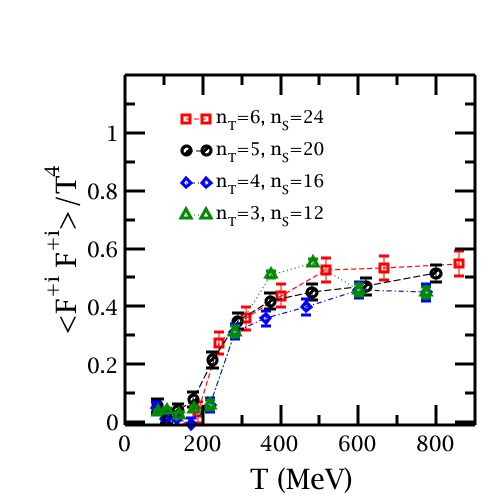
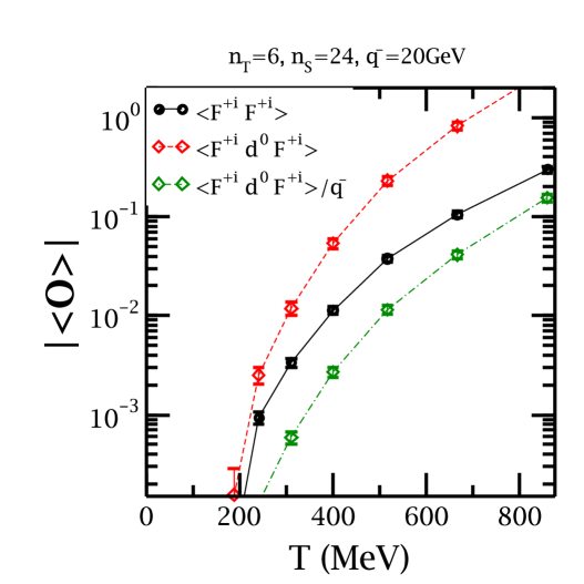
Figure 1: Left panel: The temperature dependence of the local operator $\langle F^{+i}F^{+i}\rangle$ scaled by $T^{4}$ to make it dimensionless. Right panel: temperature dependence of absolute values of the the local operator $\langle F^{+i}F^{+i}\rangle$ and the next-to-leading operator products $\langle\left[F^{+i}i\mathcal{D}^{4}F^{+i}\right]\rangle$ [red diamond (dashed)] and $\langle\left[F^{+i}i\mathcal{D}^{4}F^{+i}\right]/q^{-}\rangle$ [green diamond (dot dashed)].

To estimate $\hat{q}$ we use the point at $T=400$ MeV, where $\langle F^{+i}F^{+i}\rangle=0.01$ GeV⁴. We are considering a lattice with a length given by $4\times n_{t}a_{L}=4/0.4$ GeV${}^{-1}=10$ GeV^-1. This states that the maximum virtuality of a jet (with a $q^{-}=20$ GeV) which traverses such a length without undergoing radiation is given as $\mu^{2}=E/L=20/10/\sqrt{2}\simeq 1.4$ GeV². Thus $Q^{+}=1.4/40$ GeV. We can now use the formula $\hat{\bar{q}}=\frac{2\sqrt{2}\pi^{2}\alpha_{s}(\mu^{2})}{N_{c}2Q^{+}q^{-}}\langle F^{+i}F^{+i}\rangle.$ Using $\alpha_{s}(1.4\rm{GeV}^{2})=0.375$ [11], we obtain $\hat{\bar{q}}=0.134\rm{GeV}^{2}/{\rm fm}$ for an $SU(2)$ quark traversing a quenched $SU(2)$ plasma. In most phenomenological estimates one quotes the $\hat{q}$ of the gluon. If the above calculation were done for an $SU(2)$ gluon, the $\hat{q}$ would differ only by the overall Casimir factor of $C_{A}/C_{F}=2N_{c}^{2}/(N_{c}^{2}-1)=8/3$ yielding a $\hat{q}_{G}=0.358$ GeV²/fm, at a $T\sim 400$ MeV (Note, this value is different from that in Ref. [8] by a factor of 4, due to the neglect of this factor in that reference).

References

- [1] M. Gyulassy, X.-N. Wang, Multiple collisions and induced gluon bremsstrahlung in qcd, Nucl. Phys. B420 (1994) 583–614. arXiv:nucl-th/9306003.
- [2] A. Majumder, M. Van Leeuwen, The Theory and Phenomenology of Perturbative QCD Based Jet Quenching, Prog.Part.Nucl.Phys. A66 (2011) 41–92. arXiv:1002.2206, doi:10.1016/j.ppnp.2010.09.001.
- [3] A. Majumder, B. Muller, Higher twist jet broadening and classical propagation, Phys. Rev. C77 (2008) 054903. arXiv:0705.1147, doi:10.1103/PhysRevC.77.054903.
- [4] A. Majumder, Elastic energy loss and longitudinal straggling of a hard jet, Phys. Rev. C80 (2009) 031902. arXiv:0810.4967, doi:10.1103/PhysRevC.80.031902.
- [5] B. Muller, No Pain, No Gain: Hard Probes of the Quark-Gluon Plasma Coming of Age, arXiv:1207.7302.
- [6] A. Idilbi, A. Majumder, Extending Soft-Collinear-Effective-Theory to describe hard jets in dense QCD media, Phys.Rev. D80 (2009) 054022. arXiv:0808.1087, doi:10.1103/PhysRevD.80.054022.
- [7] M. Benzke, N. Brambilla, M. A. Escobedo, A. Vairo, Gauge invariant definition of the jet quenching parameter, arXiv:1208.4253.
- [8] A. Majumder, Calculating the Jet Quenching Parameter in Lattice Gauge Theory, arXiv:1202.5295.
- [9] J. Engels, F. Karsch, H. Satz, I. Montvay, High Temperature SU(2) Gluon Matter on the Lattice, Phys.Lett. B101 (1981) 89. doi:10.1016/0370-2693(81)90497-4.
- [10] M. Creutz, Quarks, Gluons and Lattices, Cambridge University Press, 1984.
- [11] S. Kluth, alpha(S) from LEP, J.Phys.Conf.Ser. 110 (2008) 022023. arXiv:0709.0173, doi:10.1088/1742-6596/110/2/022023.