Primordial black hole formation from non-Gaussian
curvature perturbations

Abstract

We consider several early Universe models that allow for production of large curvature perturbations at small scales. As is well known, such perturbations can lead to formation of primordial black holes (PBHs). We briefly review the today’s situation with PBH constraints and then focus on two models in which strongly non-Gaussian curvature perturbations are predicted: the hybrid inflation waterfall model and the curvaton model. We show that PBH constraints on the values of curvature perturbation power spectrum amplitude are strongly dependent on the shape of perturbations and can significantly (by two orders of magnitude) deviate from the usual Gaussian limit ${\cal P}_{\zeta}\lesssim 10^{-2}$. We give examples of PBH mass spectra calculations for both inflationary models.

1 Introduction

As is well known, in models of slow-roll inflation with one scalar field the curvature perturbation originates from the vacuum fluctuations during inflationary expansion, and these fluctuations lead to practically Gaussian classical curvature perturbations with an almost flat power spectrum. However, it is well known also that both these features are not generic in the case of inflationary models with two (or more) scalar fields: such models can easily predict adiabatic perturbations with, e.g., a “blue” spectrum and these perturbations can be non-Gaussian [1].

Possibilities for appearing of non-Gaussian fluctuations in inflationary models with multiple scalar fields had been discussed long ago [2, 3, 4]. The time evolution of the curvature perturbation on superhorizon scales (which is allowed in multiple-field scenarios [5]) implies that, in principle, a rather large non-Gaussian signal can be generated during inflation. According to the observational data [6], the primordial curvature perturbation is Gaussian with an almost scale-independent power spectrum. So far there is only a weak indication of possible primordial non-Gaussianity [at $(2-3)\sigma$ level] from the cosmic microwave background (CMB) temperature information data (see, e.g., [7]). However, non-Gaussianity is expected to become an important probe of both the early and the late Universe in the coming years [8].

The second important feature of predictions of two-field models is that these models can lead to primordial curvature perturbations with blue spectrum (for scales which are smaller than cosmological ones) and, correspondingly, can predict the primordial black hole (PBH) production at some time after inflation. In this case, PBHs become a probe for the non-Gaussianity of cosmological perturbations [9, 10, 11, 12]. The results of PBH searches can be used to constrain the ranges of early Universe model parameters.

There are several types of two-field inflation scenarios in which detectable non-Gaussianity of the curvature perturbation can be generated: curvaton models [13, 1, 14, 15, 16], models with a non-inflaton field causing inhomogeneous reheating [17, 18], curvaton-type models of preheating (see, e.g., [19] and references therein), models of waterfall transition that ends the hybrid inflation [20, 21, 22, 23]. In these two-field models the primordial curvature perturbation $\zeta$ has two components: a contribution of the inflaton (almost Gaussian) and a contribution of the extra field. This second component is parameterized by the following way [24]

$$\zeta_{\sigma}({\bf x})=a\sigma({\bf x})+\sigma^{2}({\bf x})-\langle\sigma^{2}\rangle.$$ (1)

If $a=0$, one has a $\chi^{2}$-model. Obviously, the quadratic term can’t dominate in $\zeta$ on cosmological scales where CMB data are available. It can, however, be important on smaller scales.

In the present work we study the predictions of the PBH production for two particular two-field models: the hybrid inflation model with tachyonic instability at the end of inflation and the curvaton model. The potentially large non-Gaussianity in these models is connected with the fact that the predicted magnitude of the curvature perturbation is proportional to a square of the non-inflaton (waterfall or curvaton) field. The blue spectrum in the hybrid waterfall model can arise, e.g., through the tachyonic amplification due to the dynamical symmetry breaking [20] and, in the curvaton model, due to, e.g., supergravity effects leading to the large effective mass of the curvaton [1].

The main attention in the present paper is paid to a study of probability distribution function (PDF) of the curvature perturbation and the shape of the black hole mass function, with taking into account of the non-Gaussianity. The first general study of PDF of the curvature perturbation in curvaton model was carried out in [25].

Primordial curvature perturbation spectrum in hybrid inflation waterfall model was recently studied in [26, 27, 28, 29, 30, 31, 32, 33, 34], PBH production in this model was considered in [32, 33, 34, 35]. PBH production in curvaton scenario was studied in recent works [36, 37] (without considering the non-Gaussian effects). The approximate PBH constraints on the curvature perturbation power spectrum in the curvaton model were obtained in [34].

The plan of the paper is as follows. In Sec. 2 we briefly review the available constraints on PBH abundance that follow from different types of astrophysical and cosmological data. In Sec. 3 we present the recent limits on the amplitudes of curvature perturbation power spectrum obtained with an assumption of Gaussianity of primordial curvature perturbations. In Sec. 4 the hybrid inflation model and constraints on its parameters, coming from PBH non-observation, are discussed. In Sec. 5 we discuss the possible production of PBHs in the curvaton model and the corresponding cosmological constraints that can be obtained. Our conclusions are given in Sec. 6.

2 Available constraints on PBH abundance

There are several sources of information that allow to obtain limits on PBH abundance. In the region of $M_{BH}$ which is of most interest for us ($10^{9}\lesssim M_{BH}\lesssim 10^{38}\;$g) these limits can be divided in three groups:

(i) constraints on PBHs from big bang nucleosynthesis (due to hadron injections by PBHs [38], photodissociation of deuterium [39] and light nuclei, fragmentations of quarks and gluons evaporated by PBHs [40]), $10^{9}\lesssim M_{BH}\lesssim 10^{13}\;$g, and from influence of PBH evaporations on the CMB anisotropy, $2.5\times 10^{13}\lesssim M_{BH}\lesssim 2.5\times 10^{14}\;$g [41],

(ii) constraints on PBHs from extragalactic photon background [42], $10^{13}\lesssim M_{BH}\lesssim 10^{17}\;$g,

(iii) constraints on non-evaporating PBHs (gravitational and lensing constraints, $M_{BH}>10^{15}\;$g).

Constraints on PBHs from data on extragalactic neutrino background [43, 44], in the region $10^{11}\lesssim M_{BH}\lesssim 10^{13}\;$g, are somewhat weaker than nucleosynthesis constraints. In the PBH mass region $M_{BH}\sim 10^{35}\;$g there also exist constraints from non-observation of induced gravitational waves, which have been studied in [45, 46].

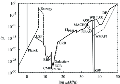
Figure 1: The available limits on PBH abundance $\beta^{\prime}(M_{BH})$ from different types of observations. The figure is taken from [41].

For a detailed review of these and other PBH constraints, see [41, 47]. Traditionally, the constraints are expressed as limits on energy density fraction of the Universe contained in PBHs at the moment of their formation, $\beta_{PBH}$, as a function of PBH mass $M_{BH}$ (it is typically assumed that

$$M_{BH}=f_{h}M_{h},$$ (2)

where $M_{h}$ is the horizon mass at the moment of PBH formation and $f_{h}$ is a constant of order of one). The summary of existing PBH limits, taken from [41], is shown in Fig. 1. This Figure gives limits in terms of $\beta^{\prime}$, which is simply related to $\beta_{PBH}$ [41]:

$$\beta^{\prime}(M_{BH})=f_{h}^{1/2}\left(\frac{g_{*}}{106.75}\right)^{-1/4}\beta_{PBH}(M_{BH}),$$ (3)

where $g_{*}$ is the effective number of relativistic degrees of freedom.

The available limits on PBH abundance, shown in the figure, can be transformed in constraints on other cosmological parameters. If, for example, inflationary model predicts large values for the curvature perturbation power spectrum at some cosmological scale, the model parameters can be constrained based on the requirement that PBHs are not over-produced.

3 PBH constraints in the Gaussian case

Several single-field inflationary models which predict a peaked power spectrum at some scale $k_{0}$ have been considered in [48, 49]. The corresponding constraints on the amplitudes of the curvature perturbation power spectrum from the non-observation of PBHs have been obtained in [46], with an assumption of Gaussian form of the perturbation distributions. It had been shown in [48] for the particular case of Coleman-Weinberg inflationary potential that non-Gaussianity of perturbations is, really, rather small. Using the assumption of Gaussianity, the PBH abundances can be calculated with a probability distribution of the form

$$p(\delta_{R})=\frac{1}{\sigma_{R}(M)\sqrt{2\pi}}\exp\left[-\frac{\delta_{R}^{2}}{2\sigma_{R}^{2}(M)}\right],$$ (4)

where $\sigma_{R}(M)$ is the mass variance (mean square deviation of density contrast $\delta$ in the sphere of comoving radius $R$), $M$ is the initial mass of fluctuation.

It is convenient to use some kind of parametrization to model the realistic peaked power spectrum of finite width. In [46] the distribution of the form

$$\lg{\cal P}_{\cal R}(k)=B+(\lg{\cal P}_{\cal R}^{0}-B)\exp\Big{[}-\frac{(\lg k/k_{0})^{2}}{2\Sigma^{2}}\Big{]}$$ (5)

was used. Here, $B\approx-8.6$, ${\cal P}_{\cal R}^{0}$ characterizes the height of the peak, $k_{0}$ is the position of the maximum and $\Sigma$ is the peak’s width. Note that comoving curvature perturbation ${\cal R}$ practically coincides with uniform density curvature perturbation $\zeta$ on super-horizon scales.

Figure 2: PBH bounds on the maximal value of primordial power spectrum, ${\cal P}_{\cal R}^{0}$, for the Gaussian case. Constraints depend on the peak’s width $\Sigma$ and its position (which corresponds to PBH mass $M_{BH}$). The figure is taken from [46].

Calculating the abundances of PBHs for different sets of model parameters, and using the available PBH limits [41], the constraints on the value of ${\cal P}_{\cal R}^{0}$ for different values of $\Sigma$ were obtained in [46]. The corresponding results are shown in Fig. 2. It is seen from this Figure that, with the assumption of Gaussianity, the resulting constraints on the power spectrum amplitude are of the order of $10^{-2}$ with some scale dependence. Similar results were also obtained recently in [47].

4 The waterfall transition model

In this section we consider the hybrid inflation model which describes an evolution of the slowly rolling inflaton field $\phi$ and the waterfall field $\chi$, with the potential [50, 51]

$$V(\phi,\chi)=\left(M^{2}-\frac{\sqrt{\lambda}}{2}\chi^{2}\right)^{2}+\frac{1}{2}m^{2}\phi^{2}+\frac{1}{2}\gamma\phi^{2}\chi^{2}.$$ (6)

The first term in Eq. (6) is a potential for the waterfall field $\chi$ with the false vacuum at $\chi=0$ and true vacuum at $\chi_{0}^{2}=2M^{2}/\sqrt{\lambda}\equiv v^{2}$. The effective mass of the waterfall field in the false vacuum state is given by

$$m_{\chi}^{2}(\phi)=\gamma\left(\phi^{2}-\phi_{c}^{2}\right),\qquad\phi_{c}^{2}\equiv\frac{2M^{2}\sqrt{\lambda}}{\gamma}.$$ (7)

At $\phi^{2}>\phi_{c}^{2}$ the false vacuum is stable, while at $\phi^{2}<\phi_{c}^{2}$ the effective mass-squared of $\chi$ becomes negative, and there is a tachyonic instability leading to a rapid growth of $\chi$-modes and eventually to an end of the inflationary expansion [30]. It is convenient to define the following parameters

$$\beta=2\sqrt{\lambda}\frac{M^{2}}{H_{c}^{2}}=\frac{|m_{\chi}^{2}(0)|}{H_{c}^{2}},\;\;\;\;\;r=\frac{3}{2}-\sqrt{\frac{9}{4}-\frac{m^{2}}{H_{c}^{2}}},$$ (8)

where $H_{c}$ is the Hubble rate during inflation.

It was shown in [33] that the magnitude of the curvature perturbation can be presented in the form

$$\zeta=\zeta_{\chi}=-A(\chi^{2}-\langle\chi^{2}\rangle),$$ (9)

where $\chi^{2}$ and $\langle\chi^{2}\rangle$ are determined at the time of an end of the waterfall, $t=t_{end}$, and $A$ is given by the integral

$$A=\int\limits_{0}^{t_{end}}\frac{H_{c}dt}{\dot{\phi}^{2}(t)+\langle\dot{\chi}^{2}(t)\rangle}\left(\frac{f(t)}{f(t_{end})}\right)^{2}\times\qquad\qquad\qquad\qquad\qquad\qquad$$

$$\times\frac{1}{2}\left[-m_{\chi}^{2}(t)+\left(\frac{\dot{f}(t)}{f(t)}\right)^{2}-\frac{\dot{p}}{\dot{\rho}}\left(m_{\chi}^{2}(t)+\left(\frac{\dot{f}(t)}{f(t)}\right)^{2}\right)\right].$$ (10)

Here, the function $f(t)$ describes the time evolution of the waterfall field (it is proportional to a numerically obtained solution of a linearized field equation for a Fourier component of a waterfall field perturbation, $\delta\chi_{k}(t)$, which is almost independent on $k$). Energy density $\rho$ and pressure $p$ are a sum of the contributions of $\phi$ and $\chi$ fields.

Figure 3: The numerically calculated spectra ${\cal P}_{\zeta}(k)$ at the moment of the end of the waterfall. Parameters used for the calculation are: $r=0.1$, $H_{c}=10^{11}\;$GeV (all curves); $\phi_{c}=3\times 10^{-6}M_{P}$ (for $\beta=1,2,7)$; $\phi_{c}=0.1M_{P}$ (for $\beta=100,1500)$. The figure is taken from [33].

It was shown in [33] that for $\beta\sim 1$ the curvature perturbation spectrum will reach values of ${\cal P}_{\zeta}\sim 1$ in a broad interval of other model parameters (such as $r$, $\gamma$, $H_{c}$). The peak values, $k_{*}$, for small $\beta$, are far beyond horizon, so, the smoothing over the horizon size will not decrease the peak values of the smoothed spectrum. The examples of the calculated power spectra for this model are shown in Fig. 3.

The relation between curvature perturbation $\zeta$ and the waterfall field value is given by Eq. (9), or, using $\sigma_{\chi}^{2}=\langle\chi^{2}\rangle$,

$$\zeta=-A(\chi^{2}-\sigma_{\chi}^{2})=\zeta_{max}-A\chi^{2},\qquad\zeta_{max}\equiv A\sigma_{\chi}^{2}.$$ (11)

Here, $A$ and $\sigma_{\chi}^{2}$ generally depend on the smoothing scale $R$. The distribution of $\chi$ is assumed to be Gaussian, i.e.,

$$p_{\chi}(\chi)=\frac{1}{\sigma_{\chi}\sqrt{2\pi}}\;e^{-\frac{\chi^{2}}{2\sigma_{\chi}^{2}}}.$$ (12)

The distribution of $\zeta$ can be easily obtained from (11, 12):

$$p_{\zeta}(\zeta)=p_{\chi}\left|\frac{d\chi}{d\zeta}\right|=\frac{1}{\sqrt{2\pi\zeta_{max}(\zeta_{max}-\zeta)}}\;e^{\frac{\zeta-\zeta_{max}}{2\zeta_{max}}},\qquad\zeta<\zeta_{max},$$ (13)

which is just a $\chi^{2}$-distribution with one degree of freedom, with an opposite sign of the argument, shifted to a value of $\zeta_{max}$. As required, $\langle\zeta\rangle=0$ and

$$\langle\zeta^{2}\rangle=\int\limits_{-\infty}^{\zeta_{max}}\zeta^{2}p_{\zeta}(\zeta)d\zeta=2\zeta_{max}^{2}.$$ (14)

On the other hand, one has

$$\langle\zeta^{2}\rangle=\sigma_{\zeta}^{2}=\int{\cal P}_{\zeta}(k)W^{2}(kR)\frac{dk}{k},$$ (15)

where $W(kR)$ is the Fourier transform of the window function, and we use a Gaussian one, $W^{2}(kR)=\exp(-k^{2}R^{2})$, in this work.

From (14, 15) we can write for $\zeta_{max}$ (we now denote the argument $R$ explicitly):

$$\zeta_{max}(R)=\left[\frac{1}{2}\int{\cal P}_{\zeta}(k)W^{2}(kR)\frac{dk}{k}\right]^{1/2}.$$ (16)

Below, we will use the following notation: $\zeta_{max}(R=0)\equiv\zeta_{max}$. So,

$$\zeta_{max}=\left[\frac{1}{2}\int{\cal P}_{\zeta}(k)\frac{dk}{k}\right]^{1/2}=\frac{1}{\sqrt{2}}\langle\zeta^{2}\rangle^{1/2}.$$ (17)

It is clear that PBHs can be produced in the early Universe, if $\zeta_{max}>\zeta_{c}$, where $\zeta_{c}$ is the threshold of PBH formation in the radiation-dominated epoch, which is to be taken from gravitational collapse model. For estimates, in the following we will use two values: $\zeta_{c}=0.75$ and $\zeta_{c}=1$ (corresponding to the PBH formation criterion in the radiation-dominated epoch: $\delta>\delta_{c}$, with $\delta_{c}=1/3$ and $\delta_{c}=0.45$, respectively) [35].

The energy density fraction of the Universe contained in collapsed objects of initial mass larger than $M$ in Press-Schechter formalism [52] is given by

$$\frac{1}{\rho_{i}}\int\limits_{M}^{\infty}\tilde{M}n(\tilde{M})d\tilde{M}=\int\limits_{\zeta_{c}}^{\infty}p_{\zeta}(\zeta)d\zeta=P(\zeta>\zeta_{c};R(M),t_{i}),$$ (18)

where function $P$ in right-hand side is the probability that in the region of comoving size $R$ the smoothed value of $\zeta$ will be larger than the PBH formation threshold value, $n(M)$ is the mass spectrum of the collapsed objects, and $\rho_{i}$ is the initial energy density. Here we ignore the dependence of the curvature perturbation $\zeta$ on time after the end of the waterfall, assuming it does not change in super-horizon regime, until the perturbations enter horizon at $k=aH$.

The horizon mass corresponding to the time when fluctuation with initial mass $M$ crosses horizon is (see [44])

$$M_{h}=M_{i}^{1/3}M^{2/3},$$ (19)

where $M_{i}$ is the horizon mass at the moment $t_{i}$,

$$M_{i}\approx\frac{4\pi}{3}t_{i}^{3}\rho_{i}\approx\frac{4\pi}{3}(H_{c}^{-1})^{3}\rho=\frac{4\pi M_{P}^{2}}{H_{c}}$$ (20)

(here, we used Friedmann equation, $\rho_{i}=3M_{P}^{2}H_{c}^{2}$). The reheating temperature of the Universe is [44]

$$T_{RH}=\left(\frac{90M_{P}^{2}H_{c}^{2}}{\pi^{2}g_{*}}\right)^{1/4},\qquad g_{*}\approx 100.$$ (21)

For simplicity, we will use the approximation that mass of the produced black hole is proportional to horizon mass [see Eq. (2)], namely,

$$M_{BH}=f_{h}M_{h}=f_{h}M_{i}^{1/3}M^{2/3},$$ (22)

where $f_{h}\approx(1/3)^{1/2}={\rm const}$.

Using (18) and (22), for the PBH number density (mass spectrum) one obtains [35]

$$n_{BH}(M_{BH})=\left(\frac{4\pi}{3}\right)^{-1/3}\left|\frac{\partial P}{\partial R}\right|\frac{f_{h}\rho_{i}^{2/3}M_{i}^{1/3}}{a_{i}M_{BH}^{2}}.$$ (23)

Considering the moment of time for which horizon mass is equal to $M_{h}$, one can obtain for the energy density fraction of Universe contained in PBHs:

$$\Omega_{PBH}(M_{h})\approx\frac{1}{\rho_{i}}\left(\frac{M_{h}}{M_{i}}\right)^{1/2}\int n_{BH}M_{BH}^{2}d\ln M_{BH}.$$ (24)

It is well known that for an almost monochromatic PBH mass spectrum, $\Omega_{PBH}(M_{h})$ coincides with the traditionally used parameter $\beta_{PBH}$. Although all PBHs do not form at the same moment of time, it is convenient to use the combination $M_{i}^{-1/2}\rho_{i}^{-1}M_{BH}^{5/2}n_{BH}(M_{BH})$ to have a feeling of how many PBHs actually form, i.e., to use the estimate following from (24)

$$M_{i}^{-1/2}\rho_{i}^{-1}M_{BH}^{5/2}n_{BH}(M_{BH})\approx\beta_{PBH}.$$ (25)

Figure 4: The PBH mass spectra for different values of the perturbation spectrum amplitudes for the hybrid inflation waterfall model. From right to left, ${\cal P}_{\zeta}^{0}=1(\zeta_{max}\approx 1.42),0.4(\zeta_{max}\approx 0.9),0.28(\zeta_{max}\approx 0.752),0.27846(\zeta_{max}\approx 0.750012),0.2784511(\zeta_{max}\approx 0.750000068)$. The position of the peak in ${\cal P}_{\zeta}(k)$-spectrum is the same for all cases. For the calculation we used the value $\tilde{\Sigma}=0.7$, and $\zeta_{c}=0.75$. The mass $M_{h}^{0}$ corresponds to horizon mass at the moment of time when perturbation with comoving wave number $k_{0}$ enters horizon. The figure is taken from [35].

Fig. 4 shows the examples of PBH mass distributions produced in the waterfall model, calculated assuming the curvature perturbation power spectrum has the form

$${\cal P}_{\zeta}(k)={\cal P}_{\zeta}^{0}\exp{\left[-\frac{(\lg{k/k_{0}})^{2}}{2\tilde{\Sigma}^{2}}\right]},$$ (26)

where ${\cal P}_{\zeta}^{0}$ gives the maximum value approached by the spectrum, $k_{0}$ is the comoving wave number corresponding to the position of the maximum and $\tilde{\Sigma}$ determines the width of the spectrum (this is just a parametrization of the result of Fig. 3).

It is seen from Fig. 4 that in the waterfall model PBH abundance severely depends on the amplitude of the curvature perturbation spectrum in a fine-tuning regime: once $\zeta_{max}$ is above $\zeta_{c}$, PBHs are produced intensively. Demanding that no excessive amount of PBHs forms in the early Universe, we can impose the bound on parameters of the inflaton potential. From the condition $\zeta_{max}<\zeta_{c}$ one has, for two fixed values of $\zeta_{c}$, the following constraints ($r=0.1$; there is a weak dependence on this parameter but the result is almost independent on $\gamma,H_{c}$):

$$\zeta_{c}=0.75:\;\;\beta>2.3,\;\;{\cal P}_{\zeta}^{0}<0.29;$$ (27)

$$\zeta_{c}=1:\;\;\beta>1.65,\;\;{\cal P}_{\zeta}^{0}<0.55.$$ (28)

One can see that the limit on the value of ${\cal P}_{\zeta}$ is significantly weaker than in the Gaussian case (see Fig. 2).

5 A case of the curvaton-type model

Curvaton is an additional to the inflaton scalar field that can be responsible (partly or fully) for generation of primordial curvature perturbations [13, 1, 14, 15, 16]. This field can also be a source of PBHs, as discussed in [53, 32].

In this work, we only consider the case of a strong positive tilt (the possibility discussed in [1, 16]) of the curvaton-generated perturbation power spectrum. At the same time, it is assumed that inflaton is responsible for generation of perturbations on cosmological scales (see Fig. 5 for an illustration).

Figure 5: A sketch that illustrates a relation between curvaton-generated and inflaton-generated curvature perturbation power spectra for the scenario of PBH production that we consider.

The curvaton field generates cosmological perturbations in two stages [1, 14, 15, 16]:

(i) Quantum fluctuations of the curvaton during inflation (at time of horizon exit) become classical, super-horizon perturbations.

(ii) In the radiation-dominated stage, the curvaton starts to oscillate (this happens at the time when Hubble parameter becomes of order of curvaton’s effective mass, $H\sim m$). The Universe at this stage becomes a mixture of radiation and matter (the curvaton behaves as a non-relativistic matter in this regime). The pressure perturbation of this mixture is non-adiabatic and the curvature perturbation is thus generated. One obtains, approximately, the expression (see, e.g., [54])

$$\zeta(t,{\bf x})=\frac{r\sigma_{\rm osc}^{\prime}}{2\sigma_{\rm osc}}\delta\sigma_{*}+\frac{r}{4}\left(\frac{\sigma_{\rm osc}^{\prime}}{\sigma_{\rm osc}}\right)^{2}\delta\sigma_{*}^{2},$$ (29)

where $r$ is the density parameter, $r=4\rho_{\sigma}/(4\rho_{r}+3\rho_{\sigma})$ ($\rho_{r}$ is the energy density of radiation after inflation), $\sigma_{\rm osc}$ is the value of the curvaton field at the onset of oscillations. The initial value for the curvaton field, $\delta\sigma_{*}$, is set by inflation. The derivative in Eq. (29) is taken with respect to the field value during inflation, $\sigma_{*}$. The term containing the second derivative, $\sigma_{\rm osc}^{\prime\prime}$, is neglected. It is assumed that $r\ll 1$.

Assuming zero average value for the curvaton field (i.e., working with the maximal box [16]), we keep in Eq. (29) only the second term,

$$\zeta(t,{\bf x})=\frac{r}{4}\left(\frac{\sigma_{\rm osc}^{\prime}}{\sigma_{\rm osc}}\right)^{2}\delta\sigma_{*}^{2}.$$ (30)

The fluctuations are strongly non-Gaussian which is not forbidden on small scales. Note that the sign of the perturbation in Eq. (30) is different from the one in Eq. (9).

The curvaton-generated curvature perturbation spectrum can be written [16] as (using the Bunch-Davies probability distribution for the perturbations of the curvaton field [55, 56])

$${\cal P}_{\zeta_{\sigma}}^{1/2}\sim\frac{2}{3}\Omega_{\sigma}t_{\sigma}^{1/2}\left(\frac{k}{k_{e}}\right)^{t_{\sigma}},$$ (31)

where $\Omega_{\sigma}=\bar{\rho}_{\sigma}/\rho$ is the relative curvaton energy density at the time of its decay (it depends on the curvaton decay rate) and

$$t_{\sigma}\cong\frac{2m_{*}^{2}}{3H_{*}^{2}}.$$ (32)

Here, $m_{*}$ is the curvaton effective mass during inflation and $H_{*}$ is the Hubble parameter.

It is rather natural (see [1] and, e.g., [57], which considers the models of chaotic inflation in supergravity) that $t_{\sigma}\sim 2/3$ which corresponds to a blue perturbation spectrum with the spectral index

$$n=1+2t_{\sigma}\sim 7/3$$ (33)

(such a situation is shown in Fig. 5). For the following, we parameterize the spectrum (31) in a simple form

$${\cal P}_{\zeta}={\cal P}_{\zeta}^{0}\left(\frac{k}{k_{e}}\right)^{n-1},\;\;k<k_{e},$$ (34)

and will treat ${\cal P}_{\zeta}^{0}$, $n$, and $k_{e}$ as free parameters. Note that $k_{e}$ does not, in general, coincide with the comoving wave number corresponding to the end of inflation. Rather, it is the scale entering horizon at the time when $\zeta$ is created [16].

Using (30) and subtracting the average value, we can write for the curvature perturbation the formula

$$\zeta=A(\delta\sigma^{2}-\langle\delta\sigma^{2}\rangle),$$ (35)

and, in analogy with the case of Eq. (13), for the distribution of $\zeta$ one obtains

$$p_{\zeta}(\zeta)=\frac{1}{\sqrt{2\pi\zeta_{min}(\zeta_{min}-\zeta)}}\;e^{\frac{\zeta-\zeta_{min}}{2\zeta_{min}}},\;\;\;{\zeta\geq\zeta_{min}},$$ (36)

where

$$\zeta_{min}=-A\langle\delta\sigma^{2}\rangle<0.$$ (37)

Note also that

$$\sigma_{\zeta}^{2}=2\zeta_{min}^{2}=\int{\cal P}_{\zeta}(k)\frac{dk}{k}.$$ (38)

The form of the distribution (36) for $\sigma_{\zeta}^{2}=2\times 10^{-4}$ is shown in Fig. 6. It is seen that in this particular case the probability to reach $\zeta\sim\zeta_{c}\sim 1$ is $\sim 10^{-20}$, i.e., of the same order as PBH constraints on $\beta^{\prime}$ of Fig. 1. Thus, the value of ${\cal P}_{\zeta}(k)\sim 10^{-4}$ is already enough to produce an observable amount of PBHs in this model (this is in agreement with the estimates of [32, 34]).

Figure 6: The form of the distribution (36) for $\sigma_{\zeta}^{2}=2\times 10^{-4}$. Dashed lines show the considered values of $\zeta_{c}$ ($0.75$ and $1$, see Sec. 4).

For a more exact estimate, we can calculate PBH mass distributions that are generated for a particular set of parameters ($n$, ${\cal P}_{\zeta}^{0}$, etc.) and then compare the resulting $\beta_{PBH}$ (using Eq. (25)) with the known limits [41] (see Fig. 1).

Figure 7: Examples of PBH mass spectra calculated for the curvaton model. The parameters used are: $n=2$, ${\cal P}_{\zeta}^{0}=4\times 10^{-4}$. For the upper curve, $\zeta_{c}=0.75$, for the lower one, $\zeta_{c}=1$. The mass $M_{h}^{0}$ corresponds to horizon mass at the moment of time when perturbation with comoving wave number $k_{e}$ enters horizon.

The example of PBH mass spectrum calculation is shown in Fig. 7. The formula (23) from the previous Section is used for this calculation (using $p_{\zeta}$ of Eq. (36) for the calculation of the probability $P$). It is seen from Fig. 7 that PBH abundances depend on particular choice of $\zeta_{c}$.

The resulting constraints on parameter ${\cal P}_{\zeta}^{0}$ (for two values of the spectral index $n$) from PBH non-observation, that were obtained in this work, are shown in Fig. 8. Thus, we see that the available constraints on the PBH abundance can be transformed into limits on the power spectrum amplitude and, subsequently, on curvaton model’s parameters, such as $\Omega_{\sigma}$. For example, comparing Fig. 8 and Eq. (31), one obtains, roughly,

$$\Omega_{\sigma}\approx({\cal P}_{\zeta}^{0})^{1/2}\lesssim 10^{-2},$$ (39)

which is already a useful constraint. It is a subject of our further study to get more exact limits for particular parameter sets of the model.

Figure 8: The limits on the maximum value of curvature perturbation power spectrum ${\cal P}_{\zeta}^{0}$ from PBH non-observation, for the curvaton model. The forbidden regions are above of the curves. $M_{h}$ is the horizon mass at the moment of time when the perturbation with comoving wave number $k_{e}$ enters horizon. The spectrum is parameterized as (34), $\zeta_{c}$=0.75.

6 Conclusions

Primordial black holes can be used to probe perturbations in our Universe at very small scales, as well as other problems of physics of early stages of the cosmological evolution. We have considered the PBH formation from primordial curvature perturbations produced in two cosmological models: in the waterfall transition in hybrid inflation scenario and in the curvaton model. Both models which were considered in the paper predict the production of strongly non-Gaussian perturbations, and non-Gaussianity was taken into account in the calculation of PBH mass spectrum (in Press-Schechter formalism).

For both models, limits on the values of perturbation power spectrum as well as constraints on inflation model parameters were obtained. The approximate constraints on the curvature perturbation spectrum amplitude follow from Eqs. (27, 28) in the case of hybrid inflation waterfall model and from Fig. 8 in the case of the curvaton models. One can conclude that the constraint on ${\cal P}_{\zeta}$ in the case of hybrid inflation waterfall model is very weak, ${\cal P}_{\zeta}\lesssim 1$. The corresponding constraint in the curvaton model is much stronger, ${\cal P}_{\zeta}\lesssim(10^{-4}-10^{-3})$, depending on the value of the spectral index and PBH mass. The PBH constraints obtained in this work confirm the estimates given in [30, 34].

References

- [1] A. D. Linde and V. F. Mukhanov, Phys. Rev. D 56 (1997) 535 [astro-ph/9610219].
- [2] D. S. Salopek, J. R. Bond and J. M. Bardeen, Phys. Rev. D 40 (1989) 1753.
- [3] D. S. Salopek, Phys. Rev. D 45 (1992) 1139.
- [4] Z. H. Fan and J. M. Bardeen, “Predictions of a nonGaussian model for large scale structure,” preprint UW-PT-92-11 (1992).
- [5] A. A. Starobinsky, JETP Lett. 42 (1985) 152 [Pisma Zh. Eksp. Teor. Fiz. 42 (1985) 124 ].
- [6] WMAP Collab. (E. Komatsu et al.), Astrophys. J. Suppl. 192 (2011) 18 [arXiv:1001.4538 [astro-ph.CO]].
- [7] A. P. S. Yadav and B. D. Wandelt, Phys. Rev. Lett. 100 (2008) 181301 [arXiv:0712.1148 [astro-ph]].
- [8] E. Komatsu, N. Afshordi, N. Bartolo et al., arXiv:0902.4759 [astro-ph.CO].
- [9] J. S. Bullock and J. R. Primack, Phys. Rev. D 55 (1997) 7423 [astro-ph/9611106].
- [10] P. Ivanov, Phys. Rev. D 57 (1998) 7145 [astro-ph/9708224].
- [11] P. Pina Avelino, Phys. Rev. D 72 (2005) 124004 [astro-ph/0510052].
- [12] J. C. Hidalgo, arXiv:0708.3875 [astro-ph].
- [13] S. Mollerach, Phys. Rev. D 42 (1990) 313.
- [14] D. H. Lyth and D. Wands, Phys. Lett. B 524 (2002) 5 [hep-ph/0110002].
- [15] T. Moroi and T. Takahashi, Phys. Lett. B 522 (2001) 215 [Erratum-ibid. B 539 (2002) 303] [hep-ph/0110096].
- [16] D. H. Lyth, J. Cosmol. Astropart. Phys. 0606 (2006) 015 [astro-ph/0602285].
- [17] G. Dvali, A. Gruzinov and M. Zaldarriaga, Phys. Rev. D 69 (2004) 023505 [arXiv:astro-ph/0303591].
- [18] L. Kofman, arXiv:astro-ph/0303614.
- [19] K. Kohri, D. H. Lyth and C. A. Valenzuela-Toledo, J. Cosmol. Astropart. Phys. 1002 (2010) 023 [Erratum-ibid. 1009 (2011) E01] [arXiv:0904.0793 [hep-ph]].
- [20] G. N. Felder, J. Garcia-Bellido, P. B. Greene, L. Kofman, A. D. Linde and I. Tkachev, Phys. Rev. Lett. 87 (2001) 011601 [hep-ph/0012142].
- [21] T. Asaka, W. Buchmuller and L. Covi, Phys. Lett. B 510 (2001) 271 [hep-ph/0104037].
- [22] E. J. Copeland, S. Pascoli and A. Rajantie, Phys. Rev. D 65 (2002) 103517 [hep-ph/0202031].
- [23] J. Garcia-Bellido, M. Garcia Perez and A. Gonzalez-Arroyo, Phys. Rev. D 67 (2003) 103501 [hep-ph/0208228].
- [24] L. Boubekeur and D. H. Lyth, Phys. Rev. D 73 (2006) 021301 [astro-ph/0504046].
- [25] M. Sasaki, J. Valiviita and D. Wands, Phys. Rev. D 74 (2006) 103003 [astro-ph/0607627].
- [26] D. H. Lyth, arXiv:1005.2461.
- [27] J. Fonseca, M. Sasaki and D. Wands, J. Cosmol. Astropart. Phys. 1009 (2010) 012 [arXiv:1005.4053].
- [28] A. A. Abolhasani and H. Firouzjahi, Phys. Rev. D 83 (2011) 063513 [arXiv:1005.2934].
- [29] J. O. Gong and M. Sasaki, J. Cosmol. Astropart. Phys. 1103 (2011) 028 [arXiv:1010.3405].
- [30] D. H. Lyth, J. Cosmol. Astropart. Phys. 1107 (2011) 035 [arXiv:1012.4617 [astro-ph.CO]].
- [31] A. A. Abolhasani, H. Firouzjahi and M. Sasaki, J. Cosmol. Astropart. Phys. 1110 (2011) 015 [arXiv:1106.6315 [astro-ph.CO]].
- [32] D. H. Lyth, arXiv:1107.1681 [astro-ph.CO].
- [33] E. Bugaev and P. Klimai, J. Cosmol. Astropart. Phys. 1111 (2011) 028 [arXiv:1107.3754 [astro-ph.CO]].
- [34] D. H. Lyth, J. Cosmol. Astropart. Phys. 1205 (2012) 022 [arXiv:1201.4312 [astro-ph.CO]].
- [35] E. Bugaev and P. Klimai, Phys. Rev. D 85 (2012) 103504 [arXiv:1112.5601 [astro-ph.CO]].
- [36] M. Kawasaki, N. Kitajima and T. T. Yanagida, arXiv:1207.2550 [hep-ph].
- [37] H. Firouzjahi, A. Green, K. Malik and M. Zarei, arXiv:1209.2652 [astro-ph.CO].
- [38] Ya. B. Zeldovich, A. A. Starobinsky, M. Yu. Khlopov and V. M. Chechetkin, Sov. Astron. Lett. 3 (1977) 110.
- [39] D. Lindley, Mon. Not. R. Astron. Soc. 193 (1980) 593.
- [40] K. Kohri and J. Yokoyama, Phys. Rev. D 61 (2000) 023501 [arXiv:astro-ph/9908160].
- [41] B. J. Carr, K. Kohri, Y. Sendouda and J. Yokoyama, Phys. Rev. D 81 (2010) 104019 [arXiv:0912.5297 [astro-ph.CO]].
- [42] D. N. Page and S. W. Hawking, Astrophys. J . 206 (1976) 1.
- [43] E. V. Bugaev and K. V. Konishchev, Phys. Rev. D 66 (2002) 084004 [arXiv:astro-ph/0206082].
- [44] E. Bugaev and P. Klimai, Phys. Rev. D 79 (2009) 103511 [arXiv:0812.4247 [astro-ph]].
- [45] R. Saito and J. Yokoyama, Phys. Rev. Lett. 102 (2009) 161101 [arXiv:0812.4339 [astro-ph]].
- [46] E. Bugaev and P. Klimai, Phys. Rev. D 83 (2011) 083521 [arXiv:1012.4697 [astro-ph.CO]].
- [47] A. S. Josan, A. M. Green and K. A. Malik, Phys. Rev. D 79 (2009) 103520 [arXiv:0903.3184 [astro-ph.CO]].
- [48] R. Saito, J. Yokoyama and R. Nagata, J. Cosmol. Astropart. Phys. 0806 (2008) 024 [arXiv:0804.3470 [astro-ph]].
- [49] E. Bugaev and P. Klimai, Phys. Rev. D 78 (2008) 063515 [arXiv:0806.4541 [astro-ph]].
- [50] A. D. Linde, Phys. Lett. B 259 (1991) 38.
- [51] A. D. Linde, Phys. Rev. D 49 (1994) 748 [astro-ph/9307002].
- [52] W. H. Press and P. Schechter, Astrophys. J. 187 (1974) 425.
- [53] K. Kohri, D. H. Lyth and A. Melchiorri, J. Cosmol. Astropart. Phys. 0804 (2008) 038 [arXiv:0711.5006 [hep-ph]].
- [54] K. Enqvist and S. Nurmi, J. Cosmol. Astropart. Phys. 0510 (2005) 013 [astro-ph/0508573].
- [55] T. S. Bunch and P. C. W. Davies, Proc. Roy. Soc. Lond. A 360 (1978) 117; A. Vilenkin and L. H. Ford, Phys. Rev. D 26 (1982) 1231; A. D. Linde, Phys. Lett. B 116 (1982) 335.
- [56] A. A. Starobinsky, Phys. Lett. B 117 (1982) 175.
- [57] V. Demozzi, A. Linde and V. Mukhanov, J. Cosmol. Astropart. Phys. 1104 (2011) 013 [arXiv:1012.0549 [hep-th]].