Coarse graining scale and effectiveness of hydrodynamic modeling

Abstract

Some basic questions about the hydrodynamical approach to relativistic heavy ion collisions are discussed aiming to clarify how far we can go with such an approach to extract useful information on the properties and dynamics of the QCD matter created. We emphasize the importance of the coarse-graining scale required for the hydrodynamic modeling which determines the space-time resolution and the associated limitations of collective flow observables. We show that certain kinds of observables can indicate the degree of inhomogeneity of the initial condition under less stringent condition than the local thermal equilibrium subjected to the coarse-graining scale compatible to the scenario.

1 Introduction

Hydrodynamic approach has shown to be very successful to describe the global and collective features of the process in relativistic heavy ion collisions. In particular, the behavior of elliptic flow parameter $v_{2}$ as function of centrality and transverse momenta data is well reproduced by hydrodynamic models PhysRevLett.86.402 ; Adams2005102 ; Adcox2005184 ; PhysRevC.72.051901 ; PhysRevC.80.024909 . It should be mentioned that other approaches based on binary collisions of constituent particles like parton cascade in general yield smaller collective flow values than the observed values. This success of hydro approach leads to the expectation that, from a detailed hydrodynamic analysis of experimental data, we may be able to determine the thermal properties of QCD matter such as the equation of state (EoS) and transport coefficients, which can be then compared to those obtained from the lattice QCD (lQCD) calculations. In fact, many works have been and are being done in this direction. Of course, these are valid and important efforts that must be done to verify how far we can go with a given working hypothesis, that is, the validity of hydrodynamics.

On the other hand, these successes brought us several new interesting questions and mysteries such as very early thermalization. The most crucial one is that why at all the hydrodynamic approach works so well for such a violent and almost microscopic collisional process. It is commonly believed that the basic hypothesis of hydrodynamics is the validity of local thermodynamical equilibrium. That is, in every space-time points, all the thermostatic state variables are well-defined and associate thermodynamic equations are valid locally. If this is true, and the hydrodynamic analysis is giving a unique scenario, then we are led to conclude that the thermalization time and correlation length are really extremely small for the QCD matter produced in the nuclear collisions. This is an important consequence for further understanding of the QCD matter at extreme conditions.

Note that in the above statement, there are two important ‘if’s, that is, ‘if really the hydrodynamics necessarily implies the local thermal equilibrium’ and ‘if the present analysis’s can be considered as a unique solution for the observed collective behavior of the relativistic heavy ion collisions’. In this paper, we would like to address these ‘if’s, and discuss what will be the experimental measure to estimate the validity of the hydrodynamic statements. In particular, it is fundamental to discover observables which are sensitive to the local dynamics of the system. We organize the present paper as follows. In Sec. II, for the sake of later bookkeeping, we make a brief review of the structure of the relativistic hydrodynamics keeping the above two if’s in mind, in particular, from the view point of the variational principle. We then discuss how the concept of coarse-graining can be introduced in the derivation of the hydrodynamic equations. It will be shown that the ideal hydrodynamic description can be considered as an effective model in terms of course-grained field variables. In Sec. III, we discuss the compatibility between the coarse-graining scale and observables. We argue that most of collective flow signals, if averaged over events, are insensitive to the detailed space-time structure of the dynamics, as far as the coarse-graining scale is compatible with these observables. The genuine local hydrodynamic signal with local thermodynamic equilibrium requires high resolution on the space-time evolution, and such an information can only be meaningful for each collisional event and not for the averaged observables. In this work, using a controlled set of initial conditions with different granularity, we look for observables which reflect the event-by-event (EbE) dynamical information and consequently are sensitive to the initial state inhomogeneity. Section IV is devoted to the discussion of our results and perspectives.

2 Relativistic Hydrodynamics

In this section, we review the derivation of relativistic hydrodynamics (mainly for the ideal case) and discuss the meaning of local thermal equilibrium in the context of coarse-graining procedure.

First, let us consider a (classical) matter carrying some conserved quantity $N$, to which four-current density $n^{\mu}(x)$ satisfies the continuity equation,

$$\partial_{\mu}n^{\mu}(x)=0.$$ (1)

In this note, to avoid unnecessary complexity for those who are not used to the “general relativistic” notations, we consider only the case of Minkowsky coordinate, $x=\{x^{0},\mathbf{x}\}$ with the metric $g_{\mu\nu}={`diag}\{1,-1,-1,-1\}$. The energy-momentum tensor $T^{\mu\nu}(x)$ of the system also conserves,

$$\partial_{\mu}T^{\mu\nu}(x)=0.\hskip 10.00002pt$$ (2)

In the case that $T^{\mu\nu}(x)$ is a $4\times 4$ symmetric matrix, e.g. in the absence of electromagnetic fields or spin variables, we can diagonalize at any point $x$. From the physical requirement, we know that there is only one time-like eigenvector $u^{\mu}$, with positive eigenvalue $\varepsilon$ LandauLifshitz ,

$$T^{\mu\nu}u_{\nu}=\varepsilon u^{\mu}.$$ (3)

We can identify this above time-like eigenvector, with proper normalization,

$$u_{\mu}u^{\mu}=1,$$ (4)

as the four-velocity for the Lorentz transformation from the observable system to the local rest frame of energy flow. Consequently, the eigenvalue $\varepsilon$ is the proper energy density, that is, the energy density measured in the rest frame of the energy flow at the space-time position $x$. The rest frame of the energy flow is called Landau-Lifshitz frame (LL). In LL frame, the energy-momentum tensor becomes:

$$T^{\mu\nu}\rightarrow[\begin{matrix}\varepsilon&\bm{0}\\ \bm{0}&\mathbb{T}\end{matrix}],$$ (5)

where $\mathbb{T}$ is the $3\times 3$ stress tensor.

In general, the direction of the energy flow vector does not necessarily coincide with that of the matter current, that is, not always $n^{\mu}\propto u^{\mu}$. In such cases, we write

$$n^{\mu}=nu^{\mu}+q^{\mu},$$ (6)

where we choose $q^{\mu}n_{\mu}=0$ so that $n$ represents the density of the conserved quantity $N$ measured in LL frame and $q^{\mu}$ is the diffusion current with respect to this frame. For the sake of later convenience, we introduce the following projection operators,

$$\Delta_{\parallel}^{\mu\nu}=u^{\mu}u^{\nu},$$ (7)

and

$$\Delta_{\perp}^{\mu\nu}=g^{\mu\nu}-u^{\mu}u^{\nu},$$ (8)

which can be used to decompose vectors or tensors systematically into the parallel and perpendicular components to the four - velocity $u^{\mu}$. For example, the above Eq.(6) is expressed formally as

$$n^{\mu}=(\Delta_{\parallel}^{\mu\nu}+\Delta_{\perp}^{\mu\nu})n_{\nu}=(n^{\nu}u_{\nu})u^{\mu}+\Delta_{\perp}^{\mu\nu}n_{\nu},$$ (9)

and identify

$$n=u_{\mu}n^{\mu},q^{\mu}=\Delta_{\perp}^{\mu\nu}n_{\nu}.$$ (10)

These projection operators can be used also to decompose the energy-momentum tensor. Due to the symmetry of $T^{\mu\nu}$, in LL frame, we can write as

$$T^{\mu\nu}=\varepsilon\Delta_{\parallel}^{\mu\nu}+\Delta_{\perp}^{\mu\alpha}\Delta_{\perp}^{\nu\beta}T_{\alpha\beta}$$ (11)

where the last term corresponds essentially to the $3\times 3$ stress tensor $\mathbb{T}$ in the local rest frame. We can further decompose the tensor $\mathbb{T}$ into isotropic irreducible parts of the local rotational symmetry as

$$\mathbb{T}=\left.\frac{1}{3}{`tr}(\mathbb{T}){\rm 1l}\right.+[\mathbbm{T}-\frac{1}{3}{`tr}(\mathbbm{T})\mathbbm{1}]$$ (12)

where $\mathbbm{1}$ is the $3\times 3$ identity matrix. This decomposition results in the original energy-momentum tensor as

$$T^{\mu\nu}=\varepsilon\Delta_{\parallel}^{\mu\nu}-P\Delta_{\perp}^{\mu\nu}+\Pi^{\mu\nu},$$ (13)

where

$$P=-\frac{1}{3}\Delta_{\perp}^{\alpha\beta}T_{\alpha\beta},.$$ (14)

Note that at this point $P$ is the dynamical pressure which is the sum of the hydrostatic pressure and bulk viscosity. And

$$\Pi^{\mu\nu}=\Delta_{\perp}^{\mu\alpha}\Delta_{\perp}^{\nu\beta}T_{\alpha\beta}-\frac{1}{3}\Delta_{\perp}^{\alpha\beta}T_{\alpha\beta}\Delta_{\perp}^{\mu\nu},$$ (15)

comes from the non-diagonal elements of the local stress tensor. $\Pi^{\mu\nu}$ is a symmetric tensor, satisfying

$$\Pi_{\mu}^{\mu}=0,u_{\mu}\Pi^{\mu\nu}=u_{\nu}\Pi^{\mu\nu}=0.$$ (16)

At this stage, the original $4\times 4$ symmetric tensor $T^{\mu\nu}$ (10 parameters) is expressed in terms of $u^{\mu},\varepsilon,P$ and $\Pi^{\mu\nu}$ (10 = 3+1+1+5). Together with the conserved current $n^{\mu}$, we have to know the time evolution of these 14 variables when their initial values are given. When the time-evolution equations form a closed system within these 14 variables, then we have defined the system of partial differential equations of (dissipative) relativistic hydrodynamics.

2.1 Ideal Fluid

In some special physical situations, the total number of variables reduces drastically. Suppose that the 3 eigenvalues of the local stress tensor are degenerated. Then $\mathbb{T}$ becomes isotropic and consequently the tensor $\Pi^{\mu\nu}$ vanishes. Furthermore, if there is no diffusion of the conserved current in LL frame, then $q^{\mu}$ also vanishes. In such a situation, the total number of variables reduces to 6. Since the conservation laws, Eqs.(1) and (2) furnish 5 equations among them, we need only one equation to close the system. Usually we introduce the so-called Equation of State (EoS) which establishes a functional relation among the local quantities, $\varepsilon,P,n$, as

$$P=P(\varepsilon,n),$$ (17)

which completes the system of ideal hydrodynamic evolution. Note that in such a system, the dynamical pressure is identified as the hydrostatic pressure. In other words, there is no bulk viscosity. More explicitly, for the set of 5 independent variables, $\varepsilon,n,\mathbf{u}$,  Eqs.(1) and (2) can be written in the form of time evolution equations as

$$\gamma\frac{d}{dt}\varepsilon=-(\varepsilon+P)\partial_{\mu}u^{\mu},$$ (18)

$$\gamma\frac{d}{dt}n=-n\partial_{\mu}u^{\mu},$$ (19)

$$\gamma n\frac{d}{dt}(\frac{\varepsilon+P}{n}u^{i})=-\partial^{i}P,$$ (20)

where $\frac{d}{dt}\varepsilon=\partial_{0}\varepsilon+v^{i}\partial_{i}\varepsilon$. Roman letters were used to denote spatial only indexes ($i=1,2,3$). This set of equations can be solved together with Eq. (17) for a given initial condition for $(\varepsilon,n,{v})$. In the equations above, $\gamma=u^{0}$ is the Lorentz factor, ${v}^{i}={u}^{i}/\gamma$ and $n^{\ast}=\gamma n$ are, respectively, the (three) velocity and the density in the global observer’s system. From now on, we use the convention that the symbol ^∗ is used to distinguish the value defined in the global observational system of the corresponding quantity without ^∗ defined in the local rest frame.

2.2 Variational Principle

We see that the hydrodynamic equation for an ideal fluid can be obtained from the continuity equations Eqs. (1) and (2) with additional assumptions such as local isotropy of the stress tensor, null diffusion of the conserved quantity in LL frame and the existence of the EoS. All these additional conditions can be satisfied if the thermodynamical equilibrium is satisfied locally. For this reason, it is commonly believed that the success of hydrodynamic description in relativistic heavy ion collisions indicates that local thermodynamical equilibrium is attained in these processes.

In fact, the set of hydrodynamic equations formally constitutes a local covariant classical field theory. If we consider that relativistic hydrodynamics as in a covariant theory, then the local thermal equilibrium should be attained in each space-time point. This is somewhat a physically contradicting condition, because to attain the thermal equilibrium, we need a large volume and time. Furthermore, even if we admit that the local thermal equilibrium could be the true answer for the success of the hydrodynamic approach in the relativistic heavy ion collisions, we don’t know yet any quantitative measure to determine the precision of the hydro predictions for the properties of the matter in question. Here, to further clarify these questions, it may be useful to derive the equations of motion for an ideal fluid dynamics from a different point of view.

Consider a small volume element $\Delta V^{\ast}$ of the fluid at the position $\mathbf{x}$, whose velocity is $\mathbf{v}$. The relativistic Lagrangian of a particle with the rest mass $m$ is given by

$$L=-m/\gamma$$ (21)

where $\gamma$ is the Lorentz factor of the particle. The four-velocity of the particle is given by

$$(u^{\mu})=(\begin{array}[c]{c}\gamma\\ \gamma\mathbf{v}\end{array}),$$ (22)

as usual.

Considering the fluid element as a particle, the intrinsic volume is $\Delta V=\Delta V^{\ast}/\gamma$ and the (average) energy density $\varepsilon$ in its rest frame is related to the rest mass of this piece of fluid as $m=\varepsilon\gamma\Delta V^{\ast}$. The Lagrangian of the fluid is then written as

$$L=\underset{x}{-\sum}\varepsilon\Delta V^{\ast}$$ (23)

where the summation is taken over every fluid element. In the limit of small volume element, we can write

$$L=-\int d^{3}x\ \varepsilon.$$ (24)

We suppose that in each fluid element, the proper energy density $\varepsilon$ can be expressed as function of the proper density $n$ of the conserved quantity as

$$\varepsilon=\varepsilon(n).$$ (25)

By definition, the current, $n^{\mu}\equiv nu^{\mu}$ conserves,

$$\partial_{\mu}n^{\mu}=0.$$ (26)

Let us then apply the variational principle for the action,

$$I=-\int d^{4}x\ \varepsilon$$ (27)

together with the constraints, Eq.(26) and the normalization condition of the four-velocity,

$$u_{\mu}u^{\mu}=1.$$ (28)

Introducing Lagrange multipliers for the constraints, we get

$$\delta\int d^{4}x\left[\varepsilon+\lambda(\partial_{\mu}n^{\mu})+\xi(u_{\mu}u^{\mu}-1)\right]=0,$$ (29)

for the variations of $(n,u^{\mu},\lambda,\xi)$. It can be shown JPhysG.25.1935 that the variational procedure leads exactly to the conservation of the energy-momentum tensor,

$$\partial_{\mu}T^{\mu\nu}=0,$$ (30)

where $T^{\mu\nu}=(\varepsilon+P)u^{\mu}u^{\nu}-Pg^{\mu\nu}$ with

$$P=n\frac{\partial\varepsilon}{\partial n}-\varepsilon.$$ (31)

Thus, the variational principle with the action Eq. (27), with the constraints, Eqs. (26) and (28) leads to the ideal hydrodynamic equations, Eqs. (18-20). Here, we showed for simplicity the case of only one conserved quantity, but it is straightforward to generalize when there are more conserved quantities, say, $\left\{n_{i},i=1,\ldots,r\right\}$. We find that everything is the same, except for the definition of the “pressure”, Eq. (31) to

$$P=\underset{i}{\sum}n_{i}\frac{\partial\varepsilon_{i}}{\partial n}-\varepsilon.$$ (32)

In the above we showed that the set of ideal hydrodynamic equations can be derived from a variational principle with the action Eq.(27). There, the most fundamental condition is that the local energy density can be expressed as function of other extensive conserved quantities,

$$\varepsilon=\varepsilon(n_{1},\ldots,n_{r}).$$ (33)

2.3 Variation in Lagrangian Coordinates

For the sake of later discussion, we will repeat the derivation of hydrodynamic equations using the Lagrangian coordinates. Let us introduce the space coordinate system $\left\{\mathbf{X}\right\}$ at the initial time $t_{0}$. We can write the fluid density distribution at this instant as

$$n_{0}=n_{0}(\mathbf{X}).$$

The fluid element initially at the position $X$ moves according to the equation of motion and occupies the other location, say $\mathbf{x}=\mathbf{r}(t;X)$. Here, $\mathbf{r}(t;X)$ represents the trajectory of the fluid element initially located at $\mathbf{X}$. Thus, the fluid configuration at the instant $t$ in the observer’s system is written as

$$n^{\ast}(\mathbf{x},t)=\int d^{3}\mathbf{X}\ n_{0}^{\ast}(\mathbf{X})\delta^{3}(\mathbf{x}-\mathbf{r}(t;\mathbf{X})),$$ (34)

which can be rewritten as

$$n^{\ast}(\mathbf{x},t)=\frac{1}{J}n_{0}^{\ast}(\mathbf{X}),$$ (35)

where

$$J={`det}(\frac{\partial\mathbf{r}}{\partial\mathbf{X}})_{\mathbf{x}=\mathbf{r}}.$$ (36)

The local proper density $n$ is then expressed as

$$n=\frac{1}{\gamma}n^{\ast}=\frac{n_{0}^{\ast}}{\gamma\ J}.$$ (37)

When $n_{0}^{\ast}$ is a smooth function, by a suitable variable transformation, we can consider $n_{0}^{\ast}$ as constant without losing generality 1751-8121-45-25-255204 .

The action Eq. (27) can be written as

$$I=\int dt\int d^{3}\mathbf{X}\ \mathcal{L}(\frac{d\mathbf{r}}{dt},\nabla_{X}\mathbf{r})$$ (38)

with the Lagrangian density

$$\mathcal{L}=-J\ \varepsilon(\frac{1}{\gamma J}n_{0}^{\ast})$$ (39)

Note that this Lagrangian density does not depend explicitly on the field $\mathbf{r}(\mathbf{X},t)$ but only on $d\mathbf{r}/dt$ and $\nabla_{X}\mathbf{r}$. The symbol $d/dt$ means the time derivative in time for a fixed $\mathbf{X}$ and $\nabla_{X}$ stands for the gradient with respect to $\mathbf{X}.$

To calculate the Euler-Lagrange equation,

$$\frac{d}{dt}\frac{\partial\mathcal{L}}{\partial(d\mathbf{r}/dt)}+\nabla_{X}(\frac{\partial\mathcal{L}}{\partial(\nabla_{X}\mathbf{r})})=0$$ (40)

we use the following properties of the Jacobian $J.$

$$\nabla_{X}\cdot\frac{\partial J}{\partial(\nabla_{X}r^{i})}=\nabla_{X}\cdot(\nabla_{X}r^{j}\times\nabla_{X}r^{k})=0,$$ (41)

and

$$\frac{\partial J}{\partial(\nabla_{X}r^{i})}\cdot\nabla_{X}=J\frac{\partial}{\partial r^{i}}.$$ (42)

In the above, the components $(i,j,k)$ of the vector $\mathbf{r}$ should be taken to be cyclic. Thus,

$$\nabla_{X}(\frac{\partial\mathcal{L}}{\partial(\nabla_{X}\mathbf{r})}) = \sum_{k}\nabla_{X}\cdot\left\{n^{2}\frac{\partial}{\partial n}\ \frac{1}{n}\varepsilon(n)\frac{\partial J}{\partial(\nabla_{X}\mathbf{r})}\right\}$$ (43)

$$= \frac{n_{0}}{n^{\ast}}\nabla_{\mathbf{r}}\ P,$$

and

$$\frac{\partial\mathcal{L}}{\partial(d\mathbf{r}/dt)} = -\frac{\partial\varepsilon}{\partial n}n^{\ast}\frac{\partial(1/\gamma)}{\partial(d\mathbf{r}/dt)}$$ (44)

$$= +\gamma\frac{d\mathbf{r}}{dt}\frac{\partial\varepsilon}{\partial n}n^{\ast}$$

$$= n_{0}\frac{\varepsilon+P}{n}\mathbf{u}$$

so that we get

$$\frac{d}{dt}(\frac{\varepsilon+P}{n}\ \mathbf{u})=-\frac{1}{n^{\ast}}\nabla_{\mathbf{r}}\ P$$ (45)

which is exactly the relativistic Euler equation, Eq.(20). Here, as before, we defined $P$ as

$$P\equiv\frac{\partial\varepsilon}{\partial n}n-\varepsilon,$$

given Eq.(25).

An important fact is that, the canonical momentum field of $\mathbf{r}(t,\mathbf{X})$ is

$$\mathbf{\pi}=\frac{\partial\mathcal{L}}{\partial(d\mathbf{r}/dt)}=\frac{\varepsilon+P}{n}\ \mathbf{u},$$ (46)

so that the Hamiltonian of the system is given by

$$H = \int d^{3}\mathbf{X}\ n_{0}^{\ast}\left[\frac{\varepsilon+P}{n}\ \mathbf{u}\right]\frac{d\mathbf{r}}{dt}-L$$ (47)

$$= \int d^{3}\mathbf{x}\ \left[(\varepsilon+P)\ \mathbf{u}^{2}+\varepsilon\right]$$

$$= \int d^{3}\mathbf{x}\ T^{00},$$

which means that the Hamiltonian density in $x$ coordinates is given by the $(00)$ component of the energy-momentum tensor, $T^{\mu\nu}=(\varepsilon+P)u^{\mu}u^{\nu}-Pg^{\mu\nu}$, as expected.

Furthermore, the total momentum $\mathbf{P}$ of the system is given by

$$\mathbf{P} = \int d\mathbf{X}\ n_{0}^{\ast}\left[\frac{\varepsilon+P}{n}\ \mathbf{u}\right]$$ (48)

$$= \int d^{3}\mathbf{x}\ (\varepsilon+P)\gamma\mathbf{u}\$$

which is nothing but the integral of the space part of $T^{0i}=(\varepsilon+P)u^{0}u^{i}$. Thus, the expression from the definition of the Hamiltonian density is:

$$\ T^{00}=(\varepsilon+P)\ \mathbf{u}^{2}+\varepsilon$$ (49)

can be rewritten as

$$T^{00}u_{0}+T^{0i}u_{i}-\varepsilon u^{0}=0.$$ (50)

Note that this is exactly the 0-th component of the eigenvalue equation Eq.(3).

2.4 Coarse Graining and Hydrodynamic Modeling

In the derivations above, we have assumed that the relation in Eq. (25) (or the general case Eq. (33)) is valid locally. This is somewhat a very severe condition, depending on the definition of the densities. For example, when we consider the hydrodynamical description of the relativistic heavy ion reactions, differently from the normal hydrodynamic applications for macroscopic fluids, the typical fluid element size can not be taken too much smaller than the whole system and also the time scale of the collective motion can not be much larger than that of the microscopic one. In such case fluctuations and inhomogeneities from the microscopic level are expected to be very large and relations like Eq. (25) becomes difficult to be well-defined.

On the other hand, the derivation of relativistic hydrodynamics from the variational procedure suggests that we may apply similar method for certain averaged densities over some statistical ensemble of fluid elements and still obtain the equations for average densities of conserved quantities. For example, let us consider a set of (very large number of) particles, instead of a truly continuum medium, which is also quickly moving. In this case, the density $n_{0}^{\ast}$ is a sum of Dirac delta functions so that any smooth relation with the energy density becomes meaningless. However, in most cases we do not have very precise resolution neither in space nor in time. Then we may introduce an averaged density distribution by introducing the smoothing function $W_{h}(\mathbf{x})$ instead of $\delta$ function in Eq.(34) and also take a certain time average, to define the smoothed density distribution as

$$n^{\ast}(\mathbf{x},t)=\int dt^{\prime}\int d^{3}\mathbf{X}\ n_{0}^{\ast}(\mathbf{X})\ U_{\tau}(t^{\prime}-t)W_{h}(\left|\mathbf{x}-\mathbf{r}(t^{\prime};\mathbf{X})\right|),$$ (51)

where $U_{\tau}(t)$ and $W_{h}(x)$ are smoothing positive definite functions (in mathematics are also called mollifiers which are approximations to the identity), satisfying

$$U_{\tau}(t) \rightarrow 0,\ \left|t\right|>\tau.$$ (52)

$$\int U_{\tau}(t)dt = 1,$$ (53)

$${`lim}_{\tau\rightarrow 0}\int\varphi(t)U_{\tau}(t)dt = \varphi(0),$$ (54)

$$W_{h}(\mathbf{r}) \rightarrow 0,\ \left|\mathbf{r}\right|>h.$$

$$\int W_{h}(\mathbf{r})d^{3}\mathbf{r} = 1,$$

$${`lim}_{h\rightarrow 0}\int\varphi(\mathbf{r})W_{h}(\mathbf{r})d^{3}\mathbf{r} = \varphi(\mathbf{0}),$$

where $\varphi$ is an arbitrary well-behaved function. A typical example of $U$ and $W$ is the Gaussian distribution. The positive parameters $\tau$ and $h$ are the scales of the time and space resolutions, respectively. We can also define the 3-current,

$$\mathbf{j}^{\ast}(\mathbf{x},t)=\int dt^{\prime}\int d^{3}\mathbf{X}\ n_{0}^{\ast}(\mathbf{X})\frac{d\mathbf{r}}{dt^{\prime}}(t^{\prime},\mathbf{X})U_{\tau}(t^{\prime}-t)W_{h}(\left|\mathbf{x}-\mathbf{r}(t^{\prime};\mathbf{X})\right|).$$

We can see that these averaged density and current satisfy the continuity equation,

$$\frac{\partial n^{\ast}}{\partial t} = \int dt^{\prime}\int d^{3}\mathbf{X}\ n_{0}^{\ast}(\mathbf{X})\ \frac{d}{dt}U_{\tau}(t^{\prime}-t)W_{h}(\left|\mathbf{x}-\mathbf{r}(t^{\prime};\mathbf{X})\right|)$$

$$= -\int dt^{\prime}\int d^{3}\mathbf{X}\ n_{0}^{\ast}(\mathbf{X})\ \frac{d}{dt^{\prime}}U_{\tau}(t^{\prime}-t)W_{h}(\left|\mathbf{x}-\mathbf{r}(t^{\prime};\mathbf{X})\right|)$$

$$= \int dt^{\prime}\int d^{3}\mathbf{X}\ n_{0}^{\ast}(\mathbf{X})\ U_{\tau}(t^{\prime}-t)\frac{d}{dt^{\prime}}W_{h}(\left|\mathbf{x}-\mathbf{r}(t^{\prime};\mathbf{X})\right|)$$

$$= -\int dt^{\prime}\int d^{3}\mathbf{X}\ n_{0}^{\ast}(\mathbf{X})\ U_{\tau}(t^{\prime}-t)\frac{d\mathbf{r}}{dt^{\prime}}\cdot\nabla_{x}W_{h}(\left|\mathbf{x}-\mathbf{r}(t^{\prime};\mathbf{X})\right|)$$

$$= -\nabla_{x}\cdot\mathbf{j}^{\ast}\mathbf{.}$$

Using this conserved smoothed current and density, we can derive the four-current,

$$j^{\mu}=(\begin{array}[c]{c}n^{\ast}\\ \mathbf{j}^{\ast}\end{array})$$

and the proper density,

$$n=\sqrt{j^{\nu}j_{\nu}}.$$

The smoothed four-velocity field is then defined as

$$u^{\mu}=\frac{1}{n}\ j^{\mu}.$$

Once we defined the (smoothed) velocity field above, we can consider the local rest frame at the space time point given by $x=(t,\mathbf{x})$ in terms of a Lorentz transformation $\Lambda(u)$, defined by

$$\Lambda(u)u=(\begin{array}[c]{c}1\\ 0\\ 0\\ 0\end{array}).$$

We can also introduce the smoothed energy-momentum tensor in analogous way. Let

$$T_{M}^{\mu\nu}(\mathbf{r}(R,t),t)$$

be the energy-momentum tensor associated to the matter at the space position $\mathbf{x}=\mathbf{r}(R,t)$ at time $t.$ From this, we introduce the smoothed energy-momentum tensor,

$$T^{\mu\nu}(\mathbf{x},t)=\int dt^{\prime}\int d^{3}\mathbf{x}^{\prime}\ U_{\tau}(t^{\prime}-t)W_{h}(\left|\mathbf{x}-\mathbf{x}^{\prime}\right|)T_{M}^{\mu\nu}(\mathbf{x}^{\prime},t^{\prime}).$$ (55)

As before, we can show that

$$\partial_{\mu}T^{\mu\nu}=\int dt^{\prime}\int d^{3}\mathbf{x}^{\prime}\ U_{\tau}(t^{\prime}-t)W_{h}(\left|\mathbf{x}-\mathbf{x}^{\prime}\right|)\partial_{\mu}^{\prime}T_{M}^{\mu\nu}(\mathbf{x}^{\prime},t^{\prime})=0,$$

if

$$\partial_{\mu}T_{M}^{\mu\nu}(x)=0.$$

From this smoothed energy-momentum tensor $T^{\mu\nu},$we can calculate also the smoothed proper energy-density as

$$\varepsilon\equiv u_{\mu}u_{\nu}T^{\mu\nu}.$$ (56)

The smoothed proper energy-density defined in this way is an average of the energy density viewed in the rest frame of the matter flow. The average is taken over all contributions from the matter within the range of the coarse-graining scale in space-time.

In terms of hydrodynamic modeling, we take these smoothed distributions as the dynamical variables that represent the system. For one collisional event, where every microscopic state is specified, we can calculate these hydrodynamical variables. Inversely, however, for a given set of hydrodynamical variables there may exist many different microscopic configurations that give rise to the same set of hydrodynamical variables. Let us call $\Omega$ the set of all collisional events with microscopic configurations that produce a given profile of the four-current $j^{\mu}$ at the initial time $t_{0}.$ In other words, $\Omega$ is the ensemble of events that corresponds to an identical hydrodynamical profile. If we calculate $\varepsilon$ at a given space-time point $x$ for each of the events in $\Omega,$ they do not coincide in general. This is so even for $j^{\mu}(\mathbf{x},t),$ if $t>t_{0}.$ However, if the coarse-graining size is large enough, the ensemble of microscopic matter which contribute to the hydrodynamic variables at the point $x$ can be sufficiently large enough so that we expect that $\varepsilon$ and $n$ will distribute sharply around their respective mean-values, say $\bar{\varepsilon}$ and $\bar{n},$ due to the central limit theorem. Furthermore, since $\bar{\varepsilon}$ and $\bar{n}$ are the average energy and matter densities belonging to the same fluid element specified by the coarse-graining volume, we expect that they will have a strong correlation, in such a way that they are functionally related

$$\bar{\varepsilon}=\bar{\varepsilon}(\bar{n}).$$ (57)

When we neglect the fluctuations in $\varepsilon$ and $j^{\mu},$ we may think of a physical model in terms of the averaged matter current which defines $\bar{n}^{\ast}$ and velocity field $\mathbf{\bar{v}}$ as the dynamical variable. For this, we may take the model action as

$$I=-\int d^{4}x\ \bar{\varepsilon}(\frac{1}{\gamma}\bar{n}^{\ast}).$$ (58)

The variational principle for this action establishes the ideal hydrodynamic equation of motion for the coarse-grained variables. This model describes the time evolution of the system belonging to a given statistical ensemble $\Omega,$ that is, the hydrodynamic initial condition.

When the fluctuations of hydrodynamical variables within the ensemble $\Omega$ are not negligible, the above ideal fluid modeling fails and we have to extend the hydrodynamical variable as stochastic ones. Even in this case, it is possible to construct the hydrodynamical model with the variational principle. In Ref. 1751-8121-45-25-255204 , it is shown that the variational principle for the action

$$I=I(\varepsilon,n^{\ast},\mathbf{v})$$

extended to fluctuating (stochastic) variables leads to the Navier-Stokes equation in the non-relativistic case. As expected, the fluctuation is directly related to the dissipation coefficients.

Therefore in the present vision, the viscosity is an unknown model parameter related directly to the coarse-graining scale. It may take different values than that obtained, for example, from lattice QCD calculations, except for the limiting case of thermal equilibrium. In fact, the simulations by ideal hydrodynamics with fluctuating initial conditions give rise to a similar behavior of $p_{t}$ dependence of $v_{2}$ to that of the viscous hydrodynamics HAMA2005 ; PhysRevLett.101.112301 .

It is interesting to note that, although the coarse-graining procedure defined through Eqs. (51) and (55) is neither local nor covariant, the resulting equation from the variational principle is written as if the theory is relativistically covariant.

3 Event by Event Hydrodynamics

As shown above, the ideal fluid description of heavy ion reaction can be regarded as an effective model for the coarse-grained variables for the flow based on the assumption, Eq.(57) together with the model action, Eq.(58). In this vision, the success of ideal fluid modeling in relativistic heavy ion collisions is, in short, reduced to the adequacy of the approximations contained in Eqs. (57) and (58) for collective variables. These two equations allow for much wider microscopic configurations than those restricted by the “local thermal equilibrium” condition (as defined in the introduction), usually considered as the necessary condition for the validity of a hydrodynamic description.

As we lengthy described in the previous section, the definition of hydrodynamic variables requires the coarse-graining procedure. The size of the hidden ensemble $\Omega$ depends on the coarse-graining size. The larger the size of coarse-graining is, the larger the ensemble $\Omega$ becomes. For larger $\Omega,$ the two conditions, Eqs. (57) and (58) have larger chance to be satisfied and the probability of the success of ideal fluid model increases. On the other hand, for larger coarse graining size, we loose the resolution in the space-time recognition. In terms of hydrodynamic variables, we will not be able to see the inhomogeneities in density profile that has smaller wavelength than the coarse-graining scale. This affects directly the class of observables that the model can describe. The extreme example is when the coarse-graining size is larger than the system size and time evolution. Then the ensemble $\Omega$ can be regarded as the statistical ensemble of the whole system, and the resultant system is a simple fireball model. Therefore, the thermal model for the particle ratio can be considered in this category.

The coarse-graining size is thus intimately related to the class of observables and the validity of hydrodynamic description. For some observables which do not require a precise space-time resolution of the system, hydrodynamics description with a large coarse-graining scale maybe sufficient. In such cases, the real local thermal equilibrium is not necessary for the success of the hydrodynamic description. In addition, the experimental observables are usually averaged over collision events classified in terms of configurations rather loosely defined, such as centrality, event plane, etc. This may mask the important information contained in each hydrodynamic evolution. For example, the recent studies PTPS.193.315 ; GDenicol of hydrodynamics with fluctuating initial condition on the elliptic flow $v_{2}$ indicate that the linear relation of integrated $v_{2}$ to the initial deformation parameter $\epsilon_{2}$ are quite insensitive not only to the granularity in the initial condition but also to the transport coefficients, when averaged over many events. This means that the event averaged integrated $v_{2}$ has a poor resolution for the hydrodynamic evolutions, so that the coarse-graining size of the respective hydrodynamics needs not to be small.

In order to claim that the real local hydrodynamics is valid, we need to have observables that reflect the genuine hydrodynamic profile in event by event basis. For example, remnant of a sharp shock wave propagation, if exist, would be a good observable which tells the possible coarse-graining size of the collective flow, since a shock wave Stoecker2005121 ; CasalderreySolana2006577 ; PhysRevC.78.034901 is a genuine local hydrodynamic phenomena. The shock thickness should not be larger than the coarse graining scale of the collective flow. Another example of genuine hydrodynamic signal may be the emergence of Kelvin-Helmholtz instability in longitudinal direction as suggested in PhysRevC.85.054901 .

In any case, it is extremely important to study the hydrodynamic observables in event-by-event basis, as proposed a long time ago PhysRevC.55.1455 ; Aguiar2002639 ; PhysRevLett.97.202302 ; ANDRADE2007 . Recently, thanks to the high quality experimental data, information contained in event-by-event fluctuations in hydrodynamic analysis and their physical origin are being more actively investigated PhysRevLett.103.242301 ; Wang:2012fx ; Qiu2012151 ; PhysRevC.81.054905 ; PhysRevC.83.064904 ; Schenke:2012wb ; PhysRevC.85.034907 .

The key point is that when we apply the hydrodynamic modeling, we do not know a-priori the coarse-graining scale suitable for the flow variables in the real scenario. Formally we can apply the hydrodynamic description even to very inhomogeneous initial conditions. But this requires a correspondingly small coarse-graining scale so that the hydrodynamic description breaks down eventually. Thus, the question is to know how far we can infer the initial condition inhomogeneity within the hydrodynamic modeling without knowing the coarse-graining scale actually permitted in the process.

In order to clarify the question of the validity of hydrodynamic models and the coarse-graining scale, it is essential to find out the set of observables which carry the information of the dynamical effects coming from the initial inhomogeneities. For this purpose, we take the following strategy. First, prepare initial conditions with different degree of inhomogeneities in a controlled way and study the flow dynamics from these initial conditions within an ideal fluid modeling. That is, we assume that the hydrodynamic coarse graining scale is smaller than the inhomogeneity of the given initial condition. Then, look for the final state observables which reflect directly the scale of inhomogeneity in the initial condition. Once such observables can be identified, we may look for these in experimental data. If experimental data show such observables which characterize the scale of initial state granularities, we may conclude that the coarse-graining size which still permits the fluid-dynamical description should be of the order of corresponding granularity scale revealed in the data. Furthermore, observation of such granularity observables indicate strongly the granularities in the initial condition, which should be useful clues for the initial state of dynamics created by QCD.

3.1 Effects of granularity in the initial conditions

As previously discussed, we are not able to know a priori the coarse-graining scale required for the hydrodynamic description of heavy ion collisions. On the other hand, the scale is intimately related to the space-time resolution. Therefore, if the experimental data reveals a signal that indicate the granularity scale of the initial condition in terms of the hydrodynamic variables, we can infer that the corresponding resolution, and consequently the coarse-graining scale is compatible to this resolution. In this sense, it is very important to establish such a measure which reflects the granularity scale in the initial condition within the framework of hydrodynamic modeling. For this purpose we investigate how the granularity of the initial condition affects the flow observables.

In order to analyze the granularity we propose a parametrization of the initial conditions based on the Glasma picture. Each event is described as a set of overlapping longitudinal tubes where the total energy content, $E_{t}$, and their width, $\sigma$, are taken as parameters Mota2011188 ; PTPS.193.315 . The tubes are distributed according to a wounded nucleons distribution with the constants chosen to describe Au-Au collisions at $\sqrt{s_{\rm NN}}=200$GeV/$A$.

In table 1 we show all the values that were used during our simulations. For each parameter set, we computed the 2D boost invariant hydrodynamic evolution of 2000 events. The impact parameter range was chosen as $b=$0–12fm and centrality classes were computed according to the final thermal multiplicity of pions, $N_{\pi}$. For the sake of simplicity, we compare the results of the extreme cases denoted A, B, C, and D (with decreasing level of granularity). The other simulations are used later when we systematically analyze the parameter dependency.

The granularity of the initial conditions generated by this model is controlled by the two parameters that give the shape of the transverse Gaussian distribution of each tube: $\sigma$ and $E_{t}$. More conveniently, one may also think of the peak energy density of the tube, $e=E_{t}/(2\pi\sigma^{2})$. Higher granularities are obtained by higher $e$ and smaller $\sigma$.

Table 1: Sets of parameters used for our simulations. The quantities in the header are: the tube width, $\sigma$, the total transverse energy content, $E_{t}$, the number of tubes for a central collision ($b=0$), $N^{\rm max}$, and the peak energy density of the tubes, $e$.

	$\sigma$[fm]	$E_{t}$[GeV/fm]	$N^{\rm max}$	$e$[GeV/fm3]
D	1	2.6	1000	0.41
	1	6.5	400	1.0
C	1	13	200	2.1
	0.7	2.6	1000	0.84
	0.7	6.5	400	2.1
	0.7	13	200	4.2
	0.5	2.6	1000	1.7
	0.5	6.5	400	4.1
	0.5	13	200	8.3
B	0.35	2.6	1000	3.4
	0.35	6.5	400	8.4
A	0.35	13	200	17

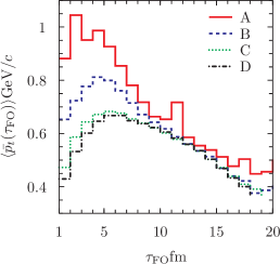
In these calculations, we observe that there is a correlation between the averaged mean-$p_{t}$ of final particles, $\langle\bar{p}_{t}\rangle$, and the instant of their freezeout, $\tau_{\rm FO}$. Figure 1 shows that the high-$p_{t}$ particles tend to be emitted earlier than those of low $p_{t}$, except for the very early times. Furthermore, this feature is enhanced by the granularity.

The result in fig.1 can be physically understood as follows. The rise of $\langle\bar{p}_{t}\rangle$ at early times is due to the initial acceleration of the fluid whose transverse velocity is set to zero at $\tau_{0}=1$fm. On the other hand, the decrease of $\langle\bar{p}_{t}\rangle$ in later times indicates that the bulk of fluid is subjected to smaller pressure gradients than the fluid elements present in the periphery – which freezeout earlier. Therefore, within the hydrodynamic picture, one may expect that the information about the space-time evolution of the system can be extracted from the $p_{t}$ dependence of flow observables.

Figure 1: Mean transverse momentum dependency on the emission time for different granularities.

3.2 NexSPheRIO

Following the idea in the previous section, we propose to calculate the flow observables for separate $p_{t}$ regions. We chose two $p_{t}$ regions denoted as low for $p_{t}=$0–0.5GeV/$c$ and high for 0.5–5 GeV/$c$. In this section, we present calculations using the NexSPheRIOmodel PhysRevC.65.054902 ; Aguiar2002639 ; HAMA2005 .

As argued before, we expect the initial geometry to be more strongly reflected in early emitted particles – which tend to have higher $p_{t}$ – than in late emitted particles – lower $p_{t}$. To check this hypothesis in a full 3D model, we have computed the flow and eccentricity phases, respectively,

$$\psi_{n}^{`A}=\frac{1}{n}`arctan\frac{\sum_{i;p_{t}\in`A}`sin(n\phi)}{\sum_{i;p_{t}\in`A}`cos(n\phi)},$$

and

$$\Psi_{n}=\frac{1}{n}`arctan\frac{\int rdrd\phi\,e(r,\phi)r^{2}`sin(n\phi)}{\int rdrd\phi\,e(r,\phi)r^{2}`cos(n\phi)},$$

where $n$ is the harmonic number, A is the $p_{t}$ range and $e(r,\phi)$ is the energy density distribution of the fluid in the initial condition. We are interested in the relative phases between the low- and high-$p_{t}$ and $\Psi_{n}$. For the sake of brevity, we will denote $\Delta\psi_{n}^{`A}=\left|\psi_{n}^{`A}-\Psi_{n}\right|$.

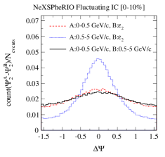
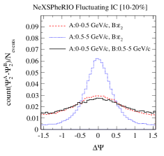
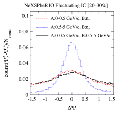
In fig.2 we show the distributions of $\Delta\psi_{2}^{\rm high}$ (dashed) and $\Delta\psi_{2}^{\rm low}$ (dotted). The top three plots show the distribution for 0–10%, 10–20% and 20–30% centrality bins, respectively. The distribution of $\Delta\psi_{2}^{\rm low}$ is peaked at $\Delta\psi=0$ but is very broad and spans over all the possible values $0$–$\pi/2$. On the other hand, $\Delta\psi_{2}^{\rm high}$ is much more concentrated around $\Delta\psi=0$. These results confirm our expectation base on the result of fig.1. We observe that the high-$p_{t}$ particles reflect better the properties of the initial condition when compared to the low-$p_{t}$ particles.

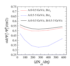
The centrality dependency of the standard deviation of the distributions, ${`std}\{\Delta\psi_{2}^{\rm high(low)}\}$, are shown in the bottom plot in fig.2. Note that ${`std}\{\Delta\psi_{2}^{\rm high}\}$ (normalized by the maximum value of $\pi/2$) reaches a minimum of 0.33 for semi-central collisions (20–30%) and is consistently lower than ${`std}\{\Delta\psi_{2}^{\rm low}\}$.

Now we use the fact that $\psi_{2}^{\rm high}$ is closely related to $\Psi_{2}$ in order to experimentally estimate $\left|\psi_{2}^{\rm low}-\Psi_{2}\right|$ by substituting $\Psi_{2}$ by the experimentally measurable quantity $\psi_{2}^{\rm high}$. The solid lines in the plots if fig.2 represent the distribution $\Delta\psi_{2}^{\rm high|low}=\left|\psi_{2}^{\rm high}-\psi_{2}^{\rm low}\right|$. Note that this quantity is in turn an experimental observable.

As expected, the distribution of $\Delta\psi_{2}^{\rm high|low}$ (solid) follows closely that of $\Delta\psi_{2}^{\rm low}$ (dotted). This indicates that one can extract experimentally the difference between the phase of the late emitted particles and the initial phase – by means of the early emitted particles. Furthermore, this difference depends on the details of space-time evolution, in particular depends on the level of granularity of the initial condition.

Figure 2: NexPSheRio results for the relative phase distributions (explained in the text).

3.3 Granularity dependence

In this section we perform a systematic study of the dependence of $\Delta\psi_{2}^{\rm high|low}$ with respect to the granularity, by changing the model parameters $\sigma$ and $E_{t}$.

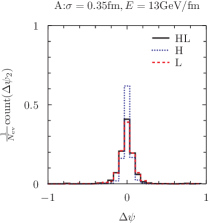
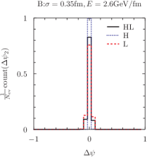
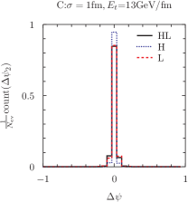
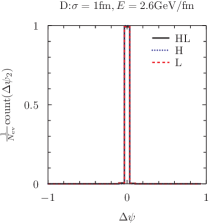
The distributions for the four parameter sets (labeled A, B, C and D in table1, with decreasing level of granularity) are presented in fig.3. For the most smooth case, D, there is no phase shift during the space-time evolution and almost all events fall in the central bin, $\Delta\psi=0$. On the other hand, for the case A, where the initial condition is the most granular among the cases we studied, there is a broad distribution of $\Delta\psi_{2}^{\rm high|low}$. This result confirms that this observable is indeed very sensitive to the initial condition granularity. Furthermore, as in the NexSPheRIO scenario, $\Delta\psi_{2}^{\rm high|low}$ follows $\Delta\psi_{2}^{\rm low}$.

Figure 3: Relative phase distributions for $\Delta\psi_{2}^{\rm high|low}$ (HL), $\Delta\psi_{2}^{\rm high}$ (H),$\Delta\psi_{2}^{\rm low}$ (L).

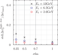
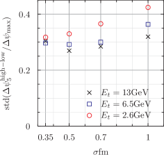
We also compute ${`std}\{\Delta\psi_{2}^{\rm high|low}\}$ for all values in table 1. The result is shown in the first plot of fig.4 as a function of the tube width, $\sigma$, for different $E_{t}$. There is a clear granularity dependence of the observable. Higher granularities – small $\sigma$ and large $E_{t}$ – produce broader distributions of ${`std}\{\Delta\psi_{2}^{\rm high|low}\}$. This suggests that the experimental analysis of this observable may provide important information about the geometrical properties of the initial condition.

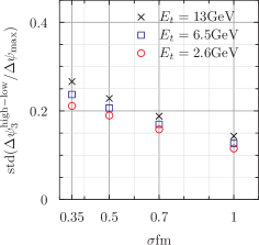
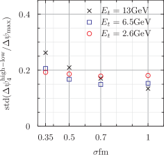
It is also argued that higher harmonics would be sensitive to smaller angular variation, thus, within this approach, we could expect a higher sensitivity to the granularity. However, since the observable proposed here is also affected by the evolution dynamics and the different freeze-out times, the result might not show a clear dependence. The granularity dependence for the higher harmonics is shown in fig.4. The higher harmonics have larger width than the elliptic case, showing that they are more sensitive for the space-time resolution, as expected. We also observe that, there is a difference in the dependence to the variation of tube energy content $E_{t}$. In the case of odd harmonics, there is no difference between the results of different $E_{t}$ configurations, whereas, in the case of even harmonics, the curves are separate. This distinction between the behavior observed for odd and even harmonics is still under investigation.

Figure 4: Granularity dependence of ${`std}\{\Delta\psi_{2}^{\rm high|low}\}$.

4 Discussion and Outlook

In this paper, we discussed the meaning of hydrodynamic modeling for the process of relativistic heavy ion collisions. We argued that it can be considered as an effective model defined by Eq.(58) for coarse grained hydrodynamic variables. There, the validity of Eq.(57) is a key point when the average over the ensemble $\Omega$ is taken.

As mentioned, the most important issue is that for the hydrodynamic modeling, we don’t know a-priori the valid coarse graining scale. The final form of relativistic hydrodynamics after the coarse-graining is a set of equations of local fields and does not have any information of the coarse-graining scale. Even if the coarse-graining size for the validity of Eq. (57) should be large, we may model the system as if the coarse-graining size is very small. Furthermore, depending on the observable, they can be very insensitive to the fluctuations in each event to extract the detailed dynamical information GDenicol . Some observables carry only information which are less affected by the coarse-graining size. On the contrary, if the behavior of an observable is well described by the hydrodynamic modeling, we can conclude that at least the coarse-graining size should be compatible with the observable. In this sense, the success of ideal hydrodynamics for the description of elliptic flow parameter $v_{2}$ tells us that the hydrodynamic coarse-graining scale must be less than that of specified by this observable.

Some specific combinations of observables analyzed in event-by-event basis can carry more detailed information on the hydrodynamic evolution of the system and many efforts are now being done using higher harmonics PhysRevC.85.024901 ; PhysRevLett.103.242301 . In the previous section, we showed another example. There, if the hydrodynamic scenario is valid even for a very spiky initial condition, particles with high momentum can be associated to the early stage of the evolution. These particles are found to be emitted from hot spots close to the surface of the system, since the time scale of expansion of such hot spot is very short. Therefore, we may consider the momentum of observed particles as a measure of time in hydrodynamic evolution. In fact, the correlations between event planes defined in momentum bins separated by the average $p_{t}$ seems very sensitive to the inhomogeneity scale of the initial condition, although, unfortunately the present analysis does not indicate still how to determine the inhomogeneity measure of the initial condition from the experimental data. However, if these observables in real experimental data, together with all other collective flow observables are consistent to a hydrodynamic model, we could say that the coarse-graining size is at least smaller than the inhomogeneity measure determined in this way.

The authors would like to thank a fruitful discussion and suggestions of G.Denicol. T.K. wishes to express his thanks for the hospitality of Prof. H. Stöcker and Prof. D. Rischke. This work has been supported by CNPq, CAPES, FAPERJ and FAPESP from Brazil and Theoretical Physics Department of the University of Frankfurt.

References

- [1] K. H. Ackermann et al. Phys. Rev. Lett., 86:402–407, Jan 2001.
- [2] J. Adams et al. Experimental and theoretical challenges in the search for the quark–gluon plasma: The star collaboration’s critical assessment of the evidence from rhic collisions. Nuclear Physics A, 757(1–2):102 – 183, 2005.
- [3] K. Adcox et al. Formation of dense partonic matter in relativistic nucleus–nucleus collisions at rhic: Experimental evaluation by the phenix collaboration. Nuclear Physics A, 757(1–2):184 – 283, 2005.
- [4] B. B. Back et al. Centrality and pseudorapidity dependence of elliptic flow for charged hadrons in au+au collisions at gev. Phys. Rev. C, 72:051901, Nov 2005.
- [5] S. Afanasiev et al. Systematic studies of elliptic flow measurements in collisions at gev. Phys. Rev. C, 80:024909, Aug 2009.
- [6] L. D. Landau and E. M. Lifshitz. Fluid Mechanics. Pergamon, New York, 1959.
- [7] Hans-Thomas Elze, Yogiro Hama, Takeshi Kodama, Martín Makler, and Johann Rafelski. Variational principle for relativistic fluid dynamics. Journal of Physics G: Nuclear and Particle Physics, 25(9):1935, 1999.
- [8] T. Koide and T. Kodama. Journal of Physics A: Mathematical and Theoretical, 45(25):255204, 2012.
- [9] Y. Hama, T. Kodama, and O. Socolowski Jr. Topics on hydrodynamic model of nucleus-nucleus collisions. Brazilian Journal of Physics, 35:24 – 51, 03 2005.
- [10] R. P. G. Andrade, F. Grassi, Y. Hama, T. Kodama, and W. L. Qian. Importance of granular structure in the initial conditions for the elliptic flow. Phys. Rev. Lett., 101:112301, Sep 2008.
- [11] Philipe Mota and Takeshi Kodama. Flow and eccentricity correlation in fluctuating initial conditions. Progress of Theoretical Physics Supplement, 193:315–318, 2012.
- [12] G.S. Denicol, H. Holopainen, P. Huovinen, H. Niemi, E. Molner, and D. Rischke. to be published.
- [13] H. Stöcker. Collective flow signals the quark-gluon plasma. Nuclear Physics A, 750(1):121 – 147, 2005.
- [14] J. Casalderrey-Solana, E.V. Shuryak, and D. Teaney. Conical flow induced by quenched qcd jets. Nuclear Physics A, 774(0):577 – 580, 2006.
- [15] G. S. Denicol, T. Kodama, T. Koide, and Ph. Mota. Shock propagation and stability in causal dissipative hydrodynamics. Phys. Rev. C, 78:034901, Sep 2008.
- [16] L. P. Csernai, D. D. Strottman, and Cs. Anderlik. Kelvin-helmholtz instability in high-energy heavy-ion collisions. Phys. Rev. C, 85:054901, May 2012.
- [17] Samya Paiva, Yogiro Hama, and Takeshi Kodama. Fluctuation effects in initial conditions for hydrodynamics. Phys. Rev. C, 55:1455–1462, Mar 1997.
- [18] C.E. Aguiar, Y. Hama, T. Kodama, and T. Osada. Event-by-event fluctuations in hydrodynamical description of heavy-ion collisions. Nuclear Physics A, 698(1–4):639 – 642, 2002.
- [19] R. Andrade, F. Grassi, Y. Hama, T. Kodama, and O. Socolowski. Examining the necessity to include event-by-event fluctuations in experimental evaluations of elliptical flow. Phys. Rev. Lett., 97:202302, Nov 2006.
- [20] R. Andrade, F. Grassi, Y. Hama, T. Kodama, and O. Socolowski Jr. Effect of event-by-event fluctuations on hydrodynamical evaluation of elliptical flow. Brazilian Journal of Physics, 37:717 – 719, 06 2007.
- [21] J. Takahashi, B. M. Tavares, W. L. Qian, R. Andrade, F. Grassi, Y. Hama, T. Kodama, and N. Xu. Topology studies of hydrodynamics using two-particle correlation analysis. Phys. Rev. Lett., 103:242301, Dec 2009.
- [22] D.J. Wang, L.P. Csernai, D. Strottman, Cs. Anderlik, Y. Cheng, et al. QGP flow fluctuations and the characteristics of higher moments. 2012.
- [23] Zhi Qiu, Chun Shen, and Ulrich Heinz. Hydrodynamic elliptic and triangular flow in pb–pb collisions at. Physics Letters B, 707(1):151 Р155, 2012.
- [24] B. Alver and G. Roland. Collision-geometry fluctuations and triangular flow in heavy-ion collisions. Phys. Rev. C, 81:054905, May 2010.
- [25] Derek Teaney and Li Yan. Triangularity and dipole asymmetry in relativistic heavy ion collisions. Phys. Rev. C, 83:064904, Jun 2011.
- [26] Bjoern Schenke, Prithwish Tribedy, and Raju Venugopalan. Fluctuating Glasma initial conditions and flow in heavy ion collisions. 2012.
- [27] Adrian Dumitru and Yasushi Nara. Scaling of fluctuations in and collisions, and eccentricities in relativistic heavy-ion collisions. Phys. Rev. C, 85:034907, Mar 2012.
- [28] Ph. Mota, T. Kodama, T. Koide, and J. Takahashi. Multi-flux tube initial condition and event-by-event hydrodynamics. Nuclear Physics A, 862–863(0):188 Р191, 2011.
- [29] H. J. Drescher, F. M. Liu, S. Ostapchenko, T. Pierog, and K. Werner. Initial condition for quark-gluon plasma evolution. Phys. Rev. C, 65:054902, Apr 2002.
- [30] Björn Schenke, Sangyong Jeon, and Charles Gale. Higher flow harmonics from d event-by-event viscous hydrodynamics. Phys. Rev. C, 85:024901, Feb 2012.