Distribution of Schmidt-like eigenvalues for Gaussian Ensembles of the Random Matrix Theory

Abstract

We analyze the form of the probability distribution function $P_{n}^{(\beta)}(w)$ of the Schmidt-like random variable $w=x_{1}^{2}/\left(\sum_{j=1}^{n}x^{2}_{j}/n\right)$, where $x_{j}$ are the eigenvalues of a given $n\times n$ $\beta$-Gaussian random matrix, $\beta$ being the Dyson symmetry index. This variable, by definition, can be considered as a measure of how any individual eigenvalue deviates from the arithmetic mean value of all eigenvalues of a given random matrix, and its distribution is calculated with respect to the ensemble of such $\beta$-Gaussian random matrices. We show that in the asymptotic limit $n\to\infty$ and for arbitrary $\beta$ the distribution $P_{n}^{(\beta)}(w)$ converges to the Marčenko-Pastur form, i.e., is defined as $P_{n}^{(\beta)}(w)\sim\sqrt{(4-w)/w}$ for $w\in[0,4]$ and equals zero outside of the support. Furthermore, for Gaussian unitary ($\beta=2$) ensembles we present exact explicit expressions for $P_{n}^{(\beta=2)}(w)$ which are valid for arbitrary $n$ and analyze their behavior.

Keywords: $\beta$-Gaussian Ensembles, Random Matrix Theory, Schmidt eigenvalues, Marčenko-Pastur law

Institute of Physics Publishing JSTAT

1 Introduction

Random covariance matrices were introduced by J. Wishart in his studies of multivariate populations [1]. In physical literature, statistical properties of the eigenvalues of random matrices have attracted a great deal of attention since the seminal works of Wigner [2], Dyson [3, 4] and Mehta [5]. Various random variables associated with eigenvalues of random matrices have been analyzed, such as, e.g., gaps in the eigenvalue spectra, number of eigenvalues in a given interval, largest or smallest eigenvalues and etc, with a special emphasis put on their typical or atypical behavior. A variety of results and their relevance to physical systems have been recently discussed in Ref. [6, 7].

One of such variables is the so-called Schmidt eigenvalue, used to characterize, e.g., the degree of entanglement of random pure states in bipartite quantum systems. It is defined as one of the eigenvalues of a given random matrix divided by the trace, i.e., the sum of all eigenvalues. On physical grounds, this variable can be therefore considered as a measure of heterogeneity of the eigenvalues and shows how any individual eigenvalue deviates from the arithmetic mean of all eigenvalues of a given random matrix. A number of significant results on the distributions of such eigenvalues and their extreme values for $\beta$-Laguerre-Wishart matrices have been obtained (see, e.g., Refs.[8, 9, 10, 11, 12] and references therein). Such random variables have also been considered recently within a different context as probes of an effective broadness of the first passage time distributions in bounded domains [13, 14].

In this paper we analyze the forms of the probability distribution function $P_{n}^{(\beta)}(w)$ of a Schmidt-like random variable

$$w=\frac{x^{2}_{1}}{\sum_{j=1}^{n}x^{2}_{j}/n}\,,$$ (1)

where $x_{j}$ are the eigenvalues of a given $n\times n$ $\beta$-Gaussian random matrix and $\beta$ is the Dyson symmetry index. Note that we use a term ”Schmidt-like random variable” since here we define $w$ as the ratio of a squared eigenvalue over the sum of all squared eigenvalues. Within such a definition $w$ is always positive definite and has a support on $[0,n]$.

The probability distribution function $P_{n}^{(\beta)}(w)$ is given by

$$P_{n}^{(\beta)}(w)=\left<\delta\left(w-\frac{nx^{2}_{1}}{\sum x^{2}_{j}}\right)\right>,$$ (2)

where the average is to be calculated with the weight

$$P(x_{1},x_{2},...,x_{n})=\frac{1}{K_{n}}\exp\left(-\frac{\beta}{2}\sum_{k=1}^{n}x_{k}^{2}\right)\prod_{j>i}|x_{j}-x_{i}|^{\beta}\,,$$ (3)

$K_{n}$ being a known normalization constant [5]. Our aim is to determine an asymptotic behavior of $P_{n}^{(\beta)}(w)$ for arbitrary $\beta$ and $n\to\infty$. Apart of this, we will present an exact, explicit results for Gaussian Unitary ($\beta=2$) Ensembles (GUE) valid for arbitrary $n$.

The paper is outlined as follows: In section 2 we provide some general results for $P_{n}^{(\beta)}(w)$ and analyze its asymptotic forms when $n\to\infty$. In section 3 we present explicit results for the distribution function of the Schmidt-like eigenvalues for GUE. Finally, in section 4 we conclude with a brief recapitulation of our results.

2 Asymptotic behavior for arbitrary $\beta$

Taking advantage of the Fourier cosine representation of the delta-function, we can conveniently rewrite Eq. (2) as

$$P_{n}^{(\beta)}(w)=\frac{2}{\pi}\int_{0}^{\infty}dy\cos(wy)\left<\cos\left(\frac{nyx^{2}_{1}}{\sum x^{2}_{j}}\right)\right>\,,$$ (4)

so that, expanding the cosine into the Taylor series, we obtain

$$P_{n}^{(\beta)}(w)=\frac{2}{\pi}\int_{0}^{\infty}dy\cos(wy)\int_{-\infty}^{\infty}dx\,\rho_{n}^{(\beta)}(x)\sum_{k=0}^{\infty}\frac{(-1)^{k}}{(2k)!}\left<\left(\frac{nyx^{2}_{1}}{\sum x^{2}_{j}}\right)^{2k}\right>\,,$$ (5)

where $\rho_{n}^{(\beta)}(x)$ is the eigenvalue density. Next, using the integral identity

$$\left(\sum x^{2}_{j}\right)^{-2k}=\frac{1}{\Gamma(2k)}\int_{0}^{\infty}d\xi\,\exp\left(-\xi\sum x^{2}_{j}\right)\xi^{2k-1}\,,$$ (6)

we can straightforwardly calculate the multiple integrals over $dx_{i}$ with $i=2,3,...n$, which yields

$$P_{n}^{(\beta)}(w)=\frac{2}{\pi}\int_{0}^{\infty}dy\,\cos(wy)\int_{-\infty}^{\infty}dx\rho_{n}^{(\beta)}(x)\sum_{k=0}^{\infty}(-1)^{k}\frac{\Gamma(f_{\beta}/2)}{(2k)!\Gamma(2k+f_{\beta}/2)}\left(\frac{\beta nyx^{2}}{2}\right)^{2k},$$ (7)

where $f_{\beta}=n+\beta n(n-1)/2$. Further on, performing the summation over $k$ in Eq. (7), we obtain

$$P_{n}^{(\beta)}(w)=\frac{\Gamma(f_{\beta}/2)}{\pi}\,\int_{0}^{\infty}dy\,\cos(wy)\int_{-\infty}^{\infty}dx\,\rho_{n}^{(\beta)}(x)\left(\mbox{\bf I}_{f_{\beta}/2-1}\left(x\sqrt{2\beta iny}\right)+cc\right)$$ (8)

where $\mbox{\bf I}_{\nu}(z)=(z/2)^{-\nu}\mbox{I}_{\nu}(z)$, $\mbox{I}_{\nu}(z)$ being the modified Bessel function, and ”cc” stands for the complex conjugate of $\mbox{\bf I}_{\nu}(z)$. Equation (8) constitutes our main general result valid for arbitrary $\beta$.

The result in Eq. (8) allows us to establish, for arbitrary $\beta$, the limiting asymptotic behavior of the distribution when $n\to\infty$. To do this, we first replace the function $\mbox{\bf I}_{\nu}(z)$ by its integral representation [15]

$$\mbox{\bf I}_{\nu}(z)=\frac{1}{\Gamma(\nu+1/2)\sqrt{\pi}}\int_{-1}^{1}dt\exp(zt)\left(1-t^{2}\right)^{\nu-1/2}\,,$$ (9)

and notice that for large values of $n$ the exponential part in the integrand in Eq. (9) is a strongly oscillating function of the argument $z$. This permits us to make the replacement $(1-t^{2})^{\nu-1/2}\approx\exp\left(-\nu t^{2}\right)$, such that after the substitution $u=t\sqrt{\nu},$ Eq. (9) becomes

$$\mbox{\bf I}_{\nu}(z)=\frac{\exp(-\frac{z^{2}}{4\nu})}{\Gamma(\nu+1/2)\sqrt{\nu\pi}}\int_{-\sqrt{\nu}}^{\sqrt{\nu}}du\exp\left(-(u-\frac{z}{2\sqrt{\nu}})^{2}\right)\approx\frac{1}{\Gamma(\nu+1/2)\sqrt{\nu}}\exp\left(-\frac{z^{2}}{4\nu}\right)\,.$$ (10)

Substituting the latter equation into Eq. (8), we arrive at the following representation

$$P_{n}^{(\beta)}(w)=\frac{2\Gamma(f_{\beta}/2)}{\pi\sqrt{f_{\beta}/2}\Gamma[(f_{\beta}-1)/2]}\int_{0}^{\infty}dy\cos(wy)\int_{-\infty}^{\infty}dx\,\rho_{n}^{(\beta)}(x)\cos\left(\frac{x^{2}\beta ny}{f_{\beta}}\right)\,,$$ (11)

which yields, after performing the integrations, the following asymptotic form

$$P_{n}^{(\beta)}(w)=\sqrt{\frac{n}{2w}}\,\rho_{n}^{(\beta)}\left(\sqrt{\frac{nw}{2}}\right)\,,$$ (12)

i.e., it simply expresses the desired probability distribution of the Schmidt-like random variable $w$ through the eigenvalue density with an appropriately rescaled variable. The asymptotic behavior of the latter is well-known and is defined by the Wigner semi-circle distribution [2, 5], so that after some very straightforward calculations we find the following asymptotic form for the normalized probability distribution function :

$$P_{\infty}^{(\beta)}(w)=\frac{1}{2\pi}\left\{\begin{array}[]{rl}\sqrt{\frac{4-w}{w}},\mbox{ for }0<w<4\,,\\ 0,\mbox{ for }w>4\,.\end{array}\right.$$ (13)

Equation (13) holds for any value of the Dyson symmetry index $\beta$. It might seem surprising at the first glance that the limiting distribution in Eq. (13) has the form of the Marčenko-Pastur law [16]. On the other hand, recall that as $n\to\infty$, the eigenvalues tend to be equidistantly-spaced so that the sum $\sum_{j}x_{j}^{2}/n$ tends to a constant. Then, it becomes clear why the distribution $P_{n}^{(\beta)}(w)$ converges to an appropriately normalized single eigenvalue density, defined by the semi-circle distribution [2, 5], so that its squared value is distributed according to the Marčenko-Pastur law.

3 Gaussian Unitary Ensemble

We turn now to the GUE case ($\beta=2$ and $f_{2}=n^{2}$), aiming to evaluate an explicit expression for the probability distribution $P_{n}^{(2)}(w)$, valid for an arbitrary value of $n$. In this case, the eigenvalue density is given by

$$\rho_{n}^{(2)}(x)=\frac{\exp(-x^{2})}{2^{n}n!\sqrt{\pi}}\left[H_{n}^{2}(x)-H_{n+1}(x)H_{n-1}(x)\right]\,,$$ (14)

where $H_{n}(x)$ denotes the Hermite polynomial [15]. Using Eqs. (9) and (14), we can represent the integral as

$$\int_{-\infty}^{\infty}dx\,\rho_{n}^{(2)}(x)\,\mbox{\bf I}_{f_{2}/2-1}\left(2x\sqrt{iny}\right)=\int_{-1}^{1}\frac{dt\left(1-t^{2}\right)^{(n^{2}-3)/2}e^{inyt^{2}}}{2^{n}n!\Gamma(n^{2}/2-1/2)\pi}f(t\sqrt{iny})\,,$$ (15)

where

$$f(t\sqrt{iny})=\int_{-\infty}^{\infty}dxe^{-(x-t\sqrt{iny})^{2}}\left[H_{n}^{2}(x)-H_{n+1}(x)H_{n-1}(x)\right].$$ (16)

Further on, this function can be expressed in terms of the associated Laguerre polynomials $L_{n}^{(\alpha)}(p)$ since for $n\geq m$ [15]

$$\int_{-\infty}^{\infty}dxe^{-(x-z)^{2}}H_{m}(x)H_{n}(x)=2^{n}\sqrt{\pi}m!z^{n-m}L_{m}^{(n-m)}(-2z^{2})\,,$$ (17)

which leads to

$$f(t\sqrt{iny})=2^{n}\sqrt{\pi}L_{n-1}^{(1)}(-2t^{2}iny),$$ (18)

where we made use of the following recurrence relation between the associated Laguerre polynomials : $nL_{n}(p)+pL_{n-1}^{(2)}(p)=L_{n-1}^{(1)}(p)$. Then, the probability distribution function $P_{n}^{(2)}(w)$ becomes

$$P_{n}^{(2)}(w)=C\int_{0}^{\infty}dy\cos(wy)\int_{0}^{1}\frac{dv}{\sqrt{v}}\left(1-v\right)^{(n^{2}-3)/2}\left(e^{inyv}L_{n-1}^{(1)}(-2inyv)+cc\right)\,,$$ (19)

where the normalization constant $C$ is given explicitly by

$$C=\frac{\pi^{-3/2}\Gamma(n^{2}/2)}{n\Gamma[(n^{2}-1)/2]}\,,$$ (20)

and $"cc"$ here stands for the complex conjugate of $\exp\left(inyv\right)L_{n-1}^{(1)}(-2inyv)$. Using next the series representation of the Laguerre polynomials, the integration over $dy$ reduces to the calculation of the following integrals

$$\sum_{0}^{n-1}a_{k}\int_{0}^{\infty}dy\cos(wy)\left[e^{inyv}(-2viny)^{k}+e^{-inyt^{2}}(2viny)^{k}\right]\,,$$ (21)

or

$$2\sum_{0}^{n-1}a_{k}\int_{0}^{\infty}dy\cos(wy)\cos\left(nyv+\frac{k\pi}{2}\right)(-2vny)^{k}\,,$$ (22)

which, using the fact that $\cos(x+k\pi/2)=\frac{d^{k}}{dx^{k}}\cos x,$ can be put into the following form

$$\pi L_{n-1}^{(1)}\left(-2v\frac{d}{dv}\right)\delta(w-nv)\,.$$ (23)

Next, the integration over $dv$ can be performed by parts, taking into account that $v^{k-1/2}(1-v)^{(n^{2}-3)/2}$ with $k>0$ vanishes at the integration limits. Then, the operator expression

$$P_{n}^{(2)}(w)=\frac{\Gamma(n^{2}/2)}{\sqrt{\pi}n^{2}\Gamma[(n^{2}-1)/2]}\left.L_{n-1}^{(1)}\left(2\frac{d}{dv}v\right)\frac{\left(1-v\right)^{(n^{2}-3)/2}}{\sqrt{v}}\right|_{v=w/n}$$ (24)

is obtained where powers of the polynomial operator are understood as $2^{j}\frac{d^{j}}{dv^{j}}v^{j}.$ Explicitly, the action of the Laguerre polynomial operator is defined as

$$L_{n-1}^{(1)}\left(2\frac{d}{dv}v\right)\frac{\left(1-v\right)^{(n^{2}-3)/2}}{\sqrt{v}}=\sum_{k=0}^{n-1}\frac{(-2)^{k}n!}{(n-1-k)!(k+1)!k!}\frac{d^{k}}{dv^{k}}\left(v^{k-1/2}\left(1-v\right)^{(n^{2}-3)/2}\right),$$ (25)

where the derivatives can be identified with the Rodrigues formula for the Jacobi polynomials $P_{n}^{(a,b)}(p)$ [15] as

$$\frac{d^{k}}{dv^{k}}\left(v^{k-1/2}\left(1-v\right)^{(n^{2}-3)/2}\right)=\frac{(-1)^{k}k!\left(1-v\right)^{(n^{2}-3)/2-k}}{\sqrt{v}}\,P_{k}^{((n^{2}-3)/2-k,-1/2)}(2v-1)\,.$$ (26)

Consequently, recalling that $v=w/n$, we find the following explicit result for the distribution $P_{n}^{(2)}(w)$ :

$$P_{n}^{(2)}(w) = \frac{\Gamma(n^{2}/2)}{\sqrt{\pi}\,\Gamma\left((n^{2}-1)/2\right)n^{3/2}}\,\frac{\left(1-w/n\right)^{(n^{2}-2n-1)/2}}{\sqrt{w}}\,\times$$ (27)

$$\times \sum_{k=0}^{n-1}{n\choose k+1}\,2^{k}\,\left(1-\frac{w}{n}\right)^{n-k-1}\,P_{k}^{((n^{2}-3)/2-k,-1/2)}\left(2\,\frac{w}{n}-1\right)\,.$$

Further on, the sum on the right-hand-side of the latter equation can be also represented, after some straightforward calculations, as a polynomial of $w$, which yields

$$P_{n}^{(2)}(w) = \frac{2\,\Gamma(n^{2}/2)}{\pi^{3/4}\,\Gamma\left((n^{2}-1)/2\right)n^{1/2}}\,\frac{\left(1-w/n\right)^{(n^{2}-2n-1)/2}}{\sqrt{w}}\,\times$$ (28)

$$\times \sum_{m=0}^{n-1}\frac{(-1)^{m}}{n^{m}}{n-1\choose m}\,\alpha_{m}\,w^{m}\,,$$

where the coefficients $\alpha_{m}$ are defined by

$$\alpha_{m}=\int^{1}_{0}\frac{\sqrt{1-t}\,dt}{\sqrt{t}}\,\left(1-2t\right)^{n-m-1}\,_{2}F_{1}\left(-m,\frac{n^{2}}{2}-1,\frac{1}{2},2t\right)\,,$$ (29)

${}_{2}F_{1}\left(\cdot\right)$ being the Gauss hypergeometric function. Equations (27) and (28) constitute our principal results for case of the Gaussian Unitary Ensemble.

Before we turn to the analysis of the asymptotic behavior of the distribution function, it might be expedient to present several first $P_{n}^{(2)}(w)$ explicitly. Below we display $P_{n}^{(2)}(w)$ for $n=2,3,4,5$ and $6$:

$$P_{2}^{(2)}(w)=\frac{1}{\pi}\frac{1}{\sqrt{(2-w)\,w}}\,,$$ (30)

$$P_{3}^{(2)}(w)=\frac{35\,(3-w)}{576\sqrt{3}\sqrt{w}}\,\Big{(}3-2\,w+3\,w^{2}\Big{)}\,,$$ (31)

$$P_{4}^{(2)}(w)=\frac{(4-w)^{7/2}}{1716\,\pi\,\sqrt{w}}\,\Big{(}12+30\,w-53\,w^{2}+38\,w^{3}\Big{)}\,,$$ (32)

$$P_{5}^{(2)}(w)=\frac{2028117\,(5-w)^{7}}{81920000000000\,\sqrt{5}\,\sqrt{w}}\,\Big{(}375-300\,w+4490\,w^{2}-5996\,w^{3}+2711\,w^{4}\Big{)}\,,$$ (33)

and

$$P_{6}^{(2)}(w)=\frac{32768\,(6-w)^{23/2}}{25113523969051155\,\pi\,\sqrt{w}}\,\Big{(}810 + 3780\,w-18090\,w^{2}$$ (34)

$$+ 52878\,w^{3}-49567\,w^{4}+16144\,w^{5}\Big{)}\,.$$

One notices that the expressions in Eqs.(30) to (34) all diverge as $1/\sqrt{w}$ when $w\to 0$. Next, all these expressions vanish (for $n>2$) as a power-law at the other edge of the support $[0,n]$, with an exponent dependent on $n$. The case $n=2$ is special: $P_{n=2}^{(2)}(w)$ diverges at both edges and has a minimum at $w=1$, which signifies that in $2\times 2$ Gaussian random matrices the two eigenvalues are most probably very different from each other. Further on, in Fig. (1) we plot these explicit forms together with more lengthy expressions for $n=7$ and $n=12$. One observes that for $w<1$ the distributions of arbitrary order are very close to the asymptotic result in Eq. (13). The distibutions are multimodal indicating a set of probable and unprobable values of $w$, which mirrors certain structuring of the eigenvalues. As $n$ gets progressively larger, the distributions become closer to the asymptotic result, Eq.  (13), for any $w\in[0,4]$. Curiously enough, despite a rather complicated form of the polynomials in the second line of Eqs. (27) and (28), they all show an appreciable variation with $w$ only for $w<4$ and are indistinguishable from zero for larger values of $w$, despite the fact that formally their support extends to larger than $4$ values of $w$.

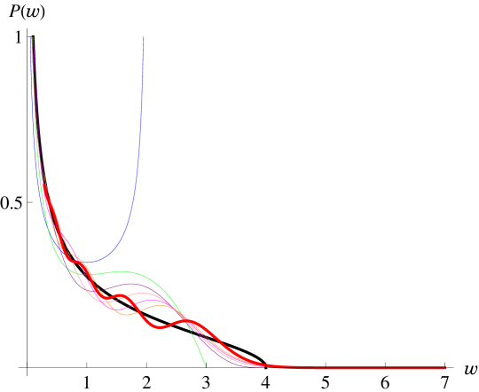
Figure 1: (color online) The distribution $P_{n}^{(2)}(w)$ in Eqs. (27) and (28) for $n=2$ (blue), $n=3$ (green), $n=4$ (purple), $n=5$ (pink), $n=6$ (magenta), $n=7$ (orange) and $n=12$ (red). Solid black line defines the asymptotic result in Eq. (13).

For arbitrary $n$, an asymptotic behavior of $P_{n}^{(2)}(w)$ for $w\ll 1$ and $w$ close to $n$ can be readily deduced from Eq. (27). As we have already remarked, one finds that for $w\to 0$, the distribution shows a generic singular behavior of the form:

$$P_{n}^{(2)}(w)\sim\frac{\Gamma\left(n^{2}/2\right)\,_{2}F_{1}\left(-n+1,\frac{1}{2},2,2\right)}{\sqrt{\pi n}\,\Gamma\left((n^{2}-1)/2\right)}\,\frac{1}{\sqrt{w}}\,,$$ (35)

where the amplitude

$$\frac{\Gamma\left(n^{2}/2\right)\,_{2}F_{1}\left(-n+1,\frac{1}{2},2,2\right)}{\sqrt{\pi n}\,\Gamma\left((n^{2}-1)/2\right)}\to\frac{1}{\pi}$$ (36)

when $n\to\infty$, in agreement with the general result in Eq. (13). This implies, in turn, that fo a given random matrix a randomly chosen eigenvalue will most probably be much less than the arithmetic mean of all eigenvalues. Further on, on the opposite extremity of the support, when $w$ is close to $n$, we have from Eq. (27) that

$$P_{n}^{(2)}(w)\sim\frac{2^{n-1}}{\sqrt{\pi}(n-1)!}\,\frac{\Gamma\left(n^{2}/2\right)}{n^{(n^{2}-2n+2)/2}\Gamma\left((n-1)^{2}/2\right)}\,\left(n-w\right)^{(n^{2}-2n-1)/2}\,,$$ (37)

i.e., $P_{n}^{(2)}(w)$ attains a zero value as a power-law when $w\to n$ with an exponent which grows in proportion to $n^{2}$ when $n\to\infty$. This implies, in turn, that for $w$ sufficiently close to $n$ the value of $P_{n}^{(2)}(w)$ decays faster than exponentially with $n$.

Finally, we address the question how the Marčenko-Pastur law in Eq. (13) can be derived from our Eq. (27). Below we briefly outline the steps involved in such a derivation. Note first that for $w<n$, one has

$$\left(1-\frac{w}{n}\right)^{(n^{2}-2n-1)/2}\to\exp\left(-\frac{nw}{2}\right)\,,$$ (38)

as $n\to\infty$, so that

$$\frac{\Gamma(n^{2}/2)}{\sqrt{\pi}\,\Gamma\left((n^{2}-1)/2\right)n^{3/2}}\,\frac{\left(1-w/n\right)^{(n^{2}-2n-1)/2}}{\sqrt{w}}\to\frac{\exp\left(-nw/2\right)}{\sqrt{2\pi nw}}\,.$$ (39)

Further on, one has that, as $n\to\infty$, [15]

$$P_{k}^{((n^{2}-3)/2-k,-1/2)}\left(2\,\frac{w}{n}-1\right)\to\frac{1}{4^{k}k!}\,H_{2k}\left(\sqrt{\frac{nw}{2}}\right)\,.$$ (40)

Using next the integral representation of the Hermite polynomials

$$H_{2k}\left(\sqrt{\frac{nw}{2}}\right)=\frac{\exp\left(nw/2\right)}{\sqrt{\pi}}\,\left(\frac{2}{nw}\right)^{k+1/2}\,\int_{0}^{\infty}dy\,y^{2k}\,\exp\left(-\frac{y^{2}}{2nw}\right)\,\cos\left(y-\pi k\right)\,,$$ (41)

we can resummate the series in Eq. (27) to find that, as $n\to\infty$, the sum in the latter equation converges to

$$\sum_{k=0}^{n-1}{n\choose k+1}\,2^{k}\,\left(1-\frac{w}{n}\right)^{n-k-1}\,P_{k}^{((n^{2}-3)/2-k,-1/2)}\left(2\,\frac{w}{n}-1\right)\to$$

$$\to\sqrt{\frac{2}{\pi nw}}\,\exp\left(\frac{nw}{2}\right)\,\int_{0}^{\infty}dy\,\exp\left(-\frac{y^{2}}{2nw}\right)\,\cos(y)\,L_{n-1}^{(1)}\left(\frac{y^{2}}{nw}\right)\,.$$ (42)

Note next that as $n\to\infty$ [15]

$$L_{n-1}^{(1)}\left(\frac{y^{2}}{nw}\right)\to\frac{n\sqrt{w}J_{1}\left(2y/\sqrt{w}\right)}{y}\,,$$ (43)

so that the integral on the right-hand-side of Eq. (3) converges to

$$\sqrt{\frac{2n}{\pi}}\,\exp\left(\frac{nw}{2}\right)\,\int_{0}^{\infty}\frac{dy}{y}\,\exp\left(-\frac{y^{2}}{2nw}\right)\,\cos(y)\,J_{1}\left(\frac{2y}{\sqrt{w}}\right)\,,$$ (44)

where $J_{1}(x)$ is the Bessel function. Noticing finally that

$$\exp\left(-\frac{y^{2}}{2nw}\right)\to 1$$ (45)

as $n\to\infty$, we can perform the integral in Eq. (44) in this limit, to get

$$\sqrt{\frac{2n}{\pi}}\,\exp\left(\frac{nw}{2}\right)\,\left\{\begin{array}[]{rl}\sqrt{1-w/4},\mbox{ for }0<w<4,\\ 0,\mbox{ for }w>4.\end{array}\right.$$ (46)

On combining the latter equation with Eq. (39), we arrive at the Marčenko-Pastur law in Eq. (13) .

4 Conclusions

To recap, we analyzed the probability distribution function $P_{n}^{(\beta)}(w)$ of the Schmidt-like random variable $w=x_{1}^{2}/\left(\sum_{j=1}^{n}x^{2}_{j}/n\right)$, Eq. (1), where $x_{j}$ are the eigenvalues of a given $n\times n$ $\beta$-Gaussian random matrix. This variable, by definition, can be considered as a measure of how any individual eigenvalue deviates from the arithmetic mean value of all eigenvalues of a given random matrix, and its distribution is calculated with respect to the ensemble of such $\beta$-Gaussian random matrices. We showed that for arbitrary Dyson symmetry index $\beta$ in the asymptotic limit $n\to\infty$ the distribution $P_{n}^{(\beta)}(w)$ converges to the Marčenko-Pastur form, i.e., is defined as $P_{n}^{(\beta)}(w)\sim\sqrt{(4-w)/w}$ for $w\in[0,4]$ and equals zero outside of the support. For Gaussian unitary ($\beta=2$) ensembles we presented exact explicit expressions for $P_{n}^{(\beta=2)}(w)$ valid for arbitrary $n$. We realised that, in general, $P_{n}^{(\beta=2)}(w)$ has a multimodal form indicating probable and unprovable values of $w$, which mirrors certain structuring of the eigenvalues. We realised that the convergence to the Marčenko-Pastur form is rather fast, so that already for $n=12$ the exact result appears to be quite close to the asymptotic form.

References

References

• [1] Wishart J (1928) Biometrika 20 A 32
• [2] Wigner E P (1951) Proc. Cambridge Philos. Soc. 47 790
• [3] Dyson F J (1962) J. Math. Phys. 3 140; 3 157; 3 166
• [4] Dyson F J and Mehta M L (1962) J. Math. Phys. 3 701
• [5] Mehta M L (2004) Random Matrices, (Academic Press, 3d Edition, London).
• [6] Bohigas O and Pato M P (2010) J. Phys. A 43 365001
• [7] Majumdar S N, Nadal C, Scadicchio A and Vivo P (2011) Phys. Rev. E 83 041105
• [8] Lloyd S and Pagels H (1988) Ann. Phys. 188 186
• [9] Kubotani H, Adachi S and Toda M (2008) Phys. Rev. Lett. 100 240501
• [10] Akemann G and Vivo P (2011) J. Stat. Mech. P05020
• [11] Vivo P (2011) J. Stat. Mech. P01022
• [12] Mejia-Monasterio C, Oshanin G and Schehr G (2011) Phys. Rev. E 84 035203
• [13] Mejia-Monasterio C, Oshanin G and Schehr G (2011) J. Stat. Mech. P06022
• [14] Mattos T G, Mejia-Monasterio C, Metzler R and Oshanin G (2012) Phys. Rev. E 86 031143
• [15] Abramowitz M and Stegun I (1965) Handbook of Mathematical Functions (New York, Dover).
• [16] Marčenko V A and Pastur L A (1967) Math. USSR-Sb. 1 457