Quasihole dynamics as a detection tool for quantum Hall phases

Abstract

Existing techniques for synthesizing gauge fields are able to bring a two-dimensional cloud of harmonically trapped bosonic atoms into a regime where the occupied single-particle states are restricted to the lowest Landau level (LLL). Repulsive short-range interactions drive various transitions from fully condensed into strongly correlated states. In these different phases we study the response of the system to quasihole excitations induced by a laser beam. We find that in the Laughlin state the quasihole performs a coherent constant rotation around the center, ensuring conservation of angular momentum. This is distinct to any other regime with higher density, where the quasihole is found to decay. At a characteristic time, the decay process is reversed, and revivals of the quasihole can be observed in the density. Measuring the period and position of the revival can be used as a spectroscopic tool to identify the strongly correlated phases in systems with a finite number of atoms.

I Introduction

Strong correlations and anyonic excitations are the intriguing properties of quantum states in two-dimensional systems exposed to strong magnetic fields. They show up in the context of fractional quantum Hall effect of electrons Laughlin (1983); Arovas et al. (1984). In recent years, the advances in techniques for cooling and controlling atoms have raised the hope that these interesting states might also be artificially generated in systems of ultracold atoms Cooper et al. (2001). This would allow to experimentally confirm the fundamental theoretical concept of fractional quantum statistics Paredes et al. (2001), and open the door for topological quantum computation Nayak et al. (2008).

The key requirement for realizing such states is a strong external gauge field, which due to the electroneutrality of the atoms has to be synthesized. Artificial gauge fields which are strong enough to bring the system into a regime, where only the lowest Landau level (LLL) is occupied, have already been generated by rotating a gas of ⁸⁷Rb Schweikhard et al. (2004). The occurrence of strongly correlated states in the LLL regime then crucially depends on the ratio between trapping energy, favoring condensation in states with small angular momentum, and the strength of repulsive interactions, which tends to spread the atoms over a wide range of angular-momentum states. In a system of bosons interacting via a two-body contact potential, this competition is known to restrict the Laughlin state Laughlin (1983) to a narrow region of parameters of extremely weak effective trapping, and thus close to the instability at the centrifugal limit Cooper (2008); Smith and Wilkin (2000); Juliá-Díaz et al. (2012). This drawback has so far hindered the experimental realization of the Laughlin state. It has led to the proposal of using laser-induced geometric phases to mimic magnetic fields (cf. Dalibard et al. (2011)). Such a method, experimentally proven in Ref. Lin et al. (2009), allows for a precise tuning of the gauge field strength as required for reaching the Laughlin state. An experimental route to produce the Laughlin state could start with preparing the system in a condensate at zero angular momentum, $L=0$. Then, stepwise transitions into states with higher angular momentum can be induced by adiabatically increasing the gauge field strength Juliá-Díaz et al. (2011, 2012), until reaching the bosonic Laughlin state, characterized by $L=N(N-1)$ (in units of $\hbar$) with $N$ the particle number.

An important question is then how to detect this state. Its zero compressibility or its constant bulk density are characterizing features, but do not uniquely distinguish the Laughlin state from other quantum liquid states. Moreover, in systems of only few particles these attributes may become quite unsharp, while experimental progress in realizing Laughlin states of few particles has been reported Gemelke et al. (2010), and even small systems have been predicted to support bulk properties like fractional excitations Juliá-Díaz et al. (2012). Thus, looking for distinctive features, experimentally accessible even in small clouds, seems to be expedient.

In this paper, we discuss a scheme for testing many-body quantum states in the LLL by piercing a quasihole into them. Experimentally, this can be achieved by focusing a laser beam onto the atomic cloud. After switching off this laser, the subsequent dynamics of the quasihole can be observed in the density of the system. We show that it yields relevant information about the underlying state. The defining property of the Laughlin state, being the densest state with zero interaction energy in a two-body contact potential, is found to be reflected in a decoherence-free dynamics of the quasihole. This is in clear contrast to the time evolution of a quasihole pierced into a state with $L<N(N-1)$. In this case, an interaction-induced dephasing delocalizes the excitation, visible in the density as a decay of the quasihole. We explicitly consider a quasihole in the $L=0$ condensate, and in a Laughlin-type quasiparticle state. For these states we show, that the decay process is reversed at a characteristic time, leading to a revival of the quasihole.

This dynamics is reminiscent of the collapse and revival of a coherent light field which resonantly interacts with a two-level atom. This effect has been studied theoretically in the framework of the Jaynes-Cummings model since the early 1980s Eberly et al. (1980); Averbukh (1992), and has experimentally been observed in systems of Rydberg atoms Rempe et al. (1987); Yeazell et al. (1990); Brune et al. (1996), or trapped ions Meekhof et al. (1996). With the realization of a Bose-Einstein condensate (BEC) in 1995, also interacting many-body systems have become candidates for studying such collapse-and-revival effects: In Ref. Lewenstein and You (1996) it has been argued that quantum fluctuations cause a phase diffusion which leads to a collapse of the macroscopic wave function. As a consequence of the discrete nature of the spectrum, periodic revivals of the macroscopic wave function have been predicted in Refs. Wright et al. (1996); Imamoḡlu et al. (1997). It has been proposed to produce macroscopic entangled states by time-evolving a condensed state Sørensen et al. (2001); Juliá-Díaz et al. (2012). An interesting scenario has been discussed in Refs. Castin and Dalibard (1997); Wright et al. (1997), studying collapse and revival of the relative phase between two spatially separate BECs. Measuring phase correlations between many BECs which are distributed on an optical lattice has allowed for observing the collapse and revival of matter waves Greiner et al. (2002). Recently, the observation of quantum state revivals has been proven to provide relevant information about the nature of multi-body interactions in a Bose condensed atomic cloud Will et al. (2010).

Also the collapse and revival which we discuss in this paper allows to extract useful information: The effect itself not only clearly distinguishes the Laughlin regime from denser ones, but also measuring the revival times and positions of the quasiholes allows to determine the kinetic and interaction contribution to the energy of the system.

Our paper is organized in the following way: After introducing the system in Sec. II, we study the coherent quasihole dynamics in the Laughlin state in Sec. III. This is in contrast to the collapse-and-revival dynamics in denser regimes described in Sec. IV. In Sec. V, we draw our conclusions.

II The system

We consider a two-dimensional system of bosonic atoms with mass $M$, described by the effective Hamiltonian ${\cal H}=\sum_{i=1}^{N}H_{i}+{\cal V}$, where the single-particle contribution reads

$$H_{i}=\frac{({\bm{p}}_{i}+{\bm{A}}_{i})^{2}}{2M}+\frac{M}{2}\omega_{\rm eff}^{2}(x^{2}+y^{2}).$$ (1)

Here, ${\bm{A}}_{i}$ denotes the artificial gauge potential acting on the $i$th particle. It shall describe a gauge field of strength $B$ perpendicular to the system. We choose the symmetric gauge, ${\bm{A}}_{i}=\frac{B}{2}(y_{i},-x_{i},0)$. Different proposals for synthesizing this gauge potential are reviewed in Refs. Cooper (2008); Dalibard et al. (2011). The trapping potential is affected by the generation of the gauge potentials, but it is possible to make the effective trap axial-symmetric with trapping frequency $\omega_{\rm eff}$. It is useful to introduce a quantity $\omega_{\perp}\equiv\sqrt{\omega_{\rm eff}^{2}+\frac{B^{2}}{4M^{2}}}$, which in the case of a rotation-induced gauge field equals the applied trapping frequency. From now on it will be used to fix units of energy, $\hbar\omega_{\perp}$, and units of length $\lambda_{\perp}=\sqrt{\hbar/(M\omega_{\perp})}$.

The first term in Eq. (1) is seen to give rise to Landau levels. Using the dimensionless parameter $\eta\equiv B/(2M\omega_{\perp})\leq 1$, we can express the Landau level gap as $\Delta_{\rm LL}=2\eta$. The degeneracy of states in each level is split by the second term in $H_{i}$. In the LLL, the eigenenergies are given by $E_{\ell}=(1-\eta)\ell+\epsilon_{0}$, corresponding to the Fock-Darwin (FD) states $\phi^{\rm FD}_{\ell}(z)\propto z^{\ell}\exp(-|z|^{2}/2)$, with $z=x+iy$, and $\ell$ the single-particle angular momentum. The term $\epsilon_{0}$ describes an $\ell$-independent zero-point energy. The interaction ${\cal V}$ is assumed to be repulsive $s$-wave scattering, described by

$${\cal V}=\frac{\hbar^{2}g}{M}\sum_{i<j}\delta^{(2)}(z_{i}-z_{j}),$$ (2)

where $g$ parametrizes the interaction strength such that $gN/4\pi$ equals the mean-field interaction energy per particle. To avoid populating higher Landau levels, we need to fulfill $gN/8\pi\ll\eta<1$. Within this constraint, we can freely tune either $g$ via Feshbach resonances, or $\eta$ by modifying the gauge field strength. This allows to drive the many-body ground state from a condensate

$$\Psi_{0}(z_{1},\dots,z_{N})\propto\prod_{i=1}^{N}\phi^{\rm FD}_{0}(z_{i})$$ (3)

for $\eta\ll 1$, to the Laughlin state

$$\Psi_{\rm L}(z_{1},\dots,z_{N})\propto\prod_{i<j}(z_{i}-z_{j})^{2}\exp(-\sum_{i}|z_{i}|^{2}/2)$$ (4)

for $\eta\rightarrow 1$ Juliá-Díaz et al. (2011).

After cooling the system into the ground state of $\cal H$, we use laser beams to pierce quasiholes into the state. In Refs. Paredes et al. (2001); Juliá-Díaz et al. (2012), it has been confirmed by exact diagonalization that a laser potential focused at position $\xi$, $V_{I}\propto I\sum_{i}\delta^{(2)}(z_{i}-\xi)$, is able to produce quasihole excitations in the Laughlin state. The laser intensity $I$ needs to be strong enough to close the gap protecting the Laughlin state. Defining a quasihole operator $\hat{\mathrm{O}}_{\rm qh}(\xi)\equiv{\cal N}\prod_{i}(z_{i}-\xi)$ which pushes away all particles from position $\xi$ and where ${\cal N}$ re-normalizes the state, the quasihole state corresponding to a state $\Psi(z_{1},\dots,z_{N})$ can generally be defined as $\Psi_{{\rm qh}}(\xi;z_{1},\dots,z_{N})=\hat{\mathrm{O}}_{\rm qh}(\xi)\Psi(z_{1},\dots,z_{N})$. This state has up to $N$ units of angular momentum more than the original state.

If the system is large enough, our procedure can be repeated in order to create several distinct quasiholes. In the following we investigate the scenario where, after generating the quasiholes, the laser beams are abruptly switched off. In general, a dynamical evolution is expected, since $\Psi_{\rm qh}$ is not an eigenstate of $\cal H$. This is directly clear for $\xi\neq 0$, where the operator $\hat{\mathrm{O}}_{\rm qh}(\xi)$ breaks the cylindrical symmetry of the Hamiltonian $\cal H$. We restrict our study to quasiholes characterized by a vanishing wave function at $\xi$, thus we do not consider the possibility of quasiholes of a different form, as for instance the half-flux excitations in the Moore-Read state Moore and Read (1991).

III Coherent quasihole dynamics in the Laughlin state

First, we consider the Laughlin state with one quasihole at position $\xi$:

$$\Psi_{{\rm L,qh}}(\xi)\equiv\hat{\mathrm{O}}_{\rm qh}(\xi)\Psi_{\rm L}={\cal N}\sum_{k=0}^{N}\xi^{N-k}f_{k}(z_{1},\dots,z_{N})\Psi_{\rm L},$$ (5)

where the $f_{k}$ are totally symmetric polynomials of $k$th order in the coordinates $z_{1},\dots,z_{N}$, with the property that each of the coordinates appears at most to linear order. Since ${\cal V}\Psi_{\rm L}=0$, we also have ${\cal V}f_{k}\Psi_{\rm L}=0$. Furthermore, all $f_{k}\Psi_{\rm L}$ are homogeneous polynomials in the $z_{i}$ times the overall Gaussian, and thus are eigenstates of the single-particle part $\sum_{i}H_{i}$ with eigenvalue $E_{k}=(1-\eta)L_{k}+N\epsilon_{0}=(1-\eta)[k+N(N-1)]+N\epsilon_{0}$. Defining $\gamma\equiv N(N-1)(1-\eta)+N\epsilon_{0}$ and $\epsilon\equiv(1-\eta)$, we can write the time evolution of the quasihole state:

$$\Psi_{\rm L,qh}(\xi,t)\equiv\mathrm{e}^{\frac{i}{\hbar}{\cal H}t}\Psi_{\rm L,qh}(\xi)={\cal N}\mathrm{e}^{\frac{i}{\hbar}\gamma t}\sum_{k=0}^{N}\mathrm{e}^{\frac{i}{\hbar}\epsilon k}\xi^{N-k}f_{k}\Psi_{\rm L}.$$ (6)

The exponential in the sum can be absorbed by making the $\xi$’s time-dependent: $\tilde{\xi}(t)\equiv\xi\mathrm{e}^{-\frac{i}{\hbar}\epsilon t}$. With this we obtain:

$$\Psi_{\rm L,qh}(\xi,t) ={\cal N}\mathrm{e}^{\frac{i}{\hbar}(\gamma+N\epsilon)t}\sum_{k=0}^{N}\tilde{\xi}(t)^{N-k}f_{k}\Psi_{\rm L}$$

$$=\mathrm{e}^{\frac{i}{\hbar}(\gamma+N\epsilon)t}\Psi_{\rm L,qh}(\tilde{\xi}(t)).$$ (7)

The overall phase evolution, $\mathrm{e}^{i(\gamma+N\epsilon)t}$, is just the dynamics of a state with a quasihole in the center, $\xi=0$, which is an eigenstate of $\cal H$. As Eq. (III) shows, for a symmetry-breaking quasihole off the center, the conservation of angular momentum is ensured by a constant coherent rotation of the quasihole around origin. Any change in $|\xi|$ is forbidden by conservation of angular momentum. The angular velocity of the quasihole is given by $\omega_{\perp}(1-\eta)$. Remarkably, no decoherence between different terms in the sum of Eq. (5) occurs during the evolution. This phenomenon is a consequence of the state’s zero interaction energy in a contact potential. Note that this behavior is in contrast to conventional fractional quantum Hall systems with long-range interactions where a tunneling of the quasihole to the edge is expected Hu et al. (2012).

The above calculation can easily be repeated for more than one quasihole. It can generally be shown that the time dependence of the corresponding wave function can be absorbed into the positions of the quasiholes $\xi_{i}\rightarrow\xi_{i}\mathrm{e}^{-\frac{i}{\hbar}\epsilon t}$, and an overall phase factor. Therefore we just have to note that the normalization factor of the wave functions, which carries the information about the anyonic statistics of the quasiholes, depends only on absolute values $|\xi_{i}|$ and $|\xi_{i}-\xi_{j}|$, thus the substitution $\xi_{i}\rightarrow\xi_{i}\mathrm{e}^{-\frac{i}{\hbar}\epsilon t}$ poses no problem there.

IV Collapse and revival of the quasihole

In contrast to the coherent dynamics of quasiholes in the Laughlin state, in this section we will encounter collapse-and-revival processes of quasiholes pierced into phases of less angular momentum, $L<N(N-1)$.

Figure 1: Contour plot of the density (divided by $N$): (a) of a $L=0$ condensate with one quasihole at $\xi=0.2$ at $t=0$ ($N$-invariant), (b) at time $t=T/2$ for $N=8$ [see definition of $T$ in Eq. (12], (c) at $t=T/2$ for $N=20$, (d) at $t=T$ ($N$-invariant).

IV.1 Quasihole in the $L=0$ condensate

We start analyzing the dynamical behavior of a quasihole in a $L=0$ condensate, described by the wave function $\Psi_{0,\rm qh}(\xi)=\hat{\mathrm{O}}_{\rm qh}(\xi)\Psi_{0}$. As before in the Laughlin case, we can decompose this expression into a sum over homogeneous polynomials, $\Psi_{0,\rm qh}(\xi)\propto\sum_{k=0}^{N}f_{k}\xi^{N-k}\Psi_{0}$, where every term is an eigenstate of the single-particle part of $\cal H$, with corresponding eigenvalue $k\epsilon+\gamma^{\prime}$. Now, $\gamma^{\prime}=N\epsilon_{0}$ is the zero-point energy. We should bear in mind that both $\epsilon$ and $\epsilon_{0}$ depend on $\eta$, so their numerical values might be different to the Laughlin case.

Again, we can absorb the single-particle contribution being linear in $k$ into the time evolution of the quasihole, so for the non-interacting system, $g=0$, we would have

$$\Psi_{0,\rm qh}(\xi,t)=\exp\left[\frac{i}{\hbar}(N\epsilon+\gamma^{\prime})t\right]\Psi_{0,\rm qh}(\tilde{\xi}(t))\,,$$ (8)

in full analogy with Eq. (III). Interactions, however, change the situation: The terms $\varphi_{k}\equiv f_{k}\Psi_{0}$ are in general not eigenstates of the interaction $\cal V$. To describe the time evolution of this system, we thus have to decompose the $\varphi_{k}$’s into an eigenbasis of $\cal V$. Since $\cal V$ conserves angular momentum, we can restrict ourselves, for every $\varphi_{k}$, to the subspace with $L=k$, for which we obtain the eigenbasis via exact diagonalization. We denote this basis by $\chi^{(k)}_{\alpha}$ and write:

$$\varphi_{k}=\sum_{\alpha}c^{(k)}_{\alpha}\chi^{(k)}_{\alpha}.$$ (9)

The coefficients $c^{(k)}_{\alpha}$ can easily be obtained: The exact diagonalization yields the $\chi^{(k)}_{\alpha}$ in the Fock basis of occupation number states $\left|n_{\ell=0},n_{\ell=1},\dots\right\rangle$. In this basis, the state $\varphi_{k}$ is represented by the vector $\left|N-k,k,0,\dots\right\rangle$, from which it differs only by a normalization factor $N_{k}=[(N-k+1)!\ (k+1)!]^{-1/2}$. We thus have $c^{(k)}_{\alpha}=N_{k}\left<\chi^{(k)}_{\alpha}\vphantom{N-k,k,0,\dots}\right|\left.N-k,k,0,\dots\vphantom{\chi^{(k)}_{\alpha}}\right>.$ The $\chi^{(k)}_{\alpha}$, being homogeneous polynomials of $k$th degree, are eigenstates of the kinetic term with the eigenvalue $k\epsilon+\gamma^{\prime}$. We now may write

$$\Psi_{0,\rm qh}(\xi,t)=\mathrm{e}^{\frac{i}{\hbar}(N\epsilon+\gamma^{\prime})t}\sum_{k=0}^{N}\tilde{\xi}(t)^{N-k}\sum_{\alpha}c^{(k)}_{\alpha}\chi^{(k)}_{\alpha}\mathrm{e}^{i\epsilon_{\alpha}^{(k)}t}.$$ (10)

Here, $\epsilon_{\alpha}^{(k)}$ is the eigenvalue of $\cal V$ corresponding to the eigenvector $\chi^{(k)}_{\alpha}$. The presence of this term causes, in general, a dephasing of the different contributions to $\Psi_{0,\rm qh}(\xi)$. Thus, while the single-particle contribution just rotates the quasihole at fixed radial position $|\xi|$, the interaction makes the quasihole fade out, as shown in the density plots of Fig. 1. Also, slight deformations of the cloud as a whole become apparent during the time evolution, in clear contrast to the Laughlin case. This interaction-driven dynamics also happens for a symmetry-conserving quasihole in the center.

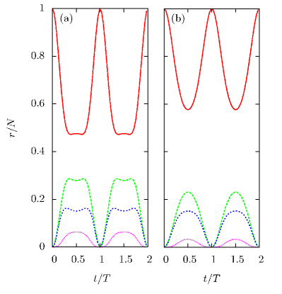
Figure 2: Eigenvalues $r$ of the one-body density matrix $\rho$ as a function of time. Initially, one hole was pierced at $\xi=0.2$ into the $L=0$ condensate. (a) $N=8$. (b) $N=20$.

To quantify the dephasing we consider the eigenvalues $r$ of the one-body density matrix $\rho_{ij}=\left\langle\Psi_{0,\rm qh}(\xi,t)\right|\hat{\mathrm{c}}_{i}^{\dagger}\hat{\mathrm{c}}_{j}\left|\Psi_{0,\rm qh}(\xi,t)\right\rangle$, that is, the occupation of the different eigenmodes. Here, $\hat{\mathrm{c}}_{i}$ ($\hat{\mathrm{c}}_{i}^{\dagger}$) is the annihilation (creation) operator of a particle in FD state $\phi_{i}^{\rm FD}$. As shown in Fig. 2, initially all particles occupy the same single-particle state, $(z-\xi)\exp(-|z|^{2}/2)$, and all eigenvalues of $\rho$ are zero except for one which is equal to the number of particles $N$. If the hole is placed in the center, the different instantaneous eigenmodes of $\rho$ are the Fock-Darwin functions, as a matter of fact that the initial state has definite angular momentum, and the Hamiltonian conserves angular momentum. For all particle numbers we have studied, the most occupied mode is, at any time, $\phi_{1}^{\rm FD}$, while the second most occupied is the Gaussian, i.e. $\phi_{0}^{\rm FD}$. As can be inferred from Fig. 2, and as we have verified explicitly by calculating the pair-correlation function Graß (2012), the time evolution brings the initially fully uncorrelated system into a correlated state, where detection of one particle at position $z$ influences the outcome of another measurement at position $z^{\prime}$. The effect is most pronounced in small systems with a quasihole in the center. In this case, we find for $N=12$ at $t=T/2$ a correlated state with almost equally populated modes, $n_{0}^{\rm FD}=4.7$ and $n_{1}^{\rm FD}=4.3$.

As seen in Figs. 1 and  2, the collapse of the quasihole is followed by a perfect revival. We thus have oscillations between fully condensed quasihole states and correlated states. In the absence of perturbations, these oscillations of period $T$ will continue forever. Note that, in general, the position of the quasihole at the $n$th revival, $\xi^{(n)}$, changes from period to period due to the kinetic contribution. In the following, we will derive expressions for $T$ and $\xi^{(n)}$, which will allow to deduce information about different system’s parameter by measuring these quantities.

Therefore, we have to analyze the spectra $\epsilon_{\alpha}^{(k)}$, which define the periods $\tilde{T}_{\alpha}^{(k)}=2\pi\hbar/\epsilon_{\alpha}^{(k)}$ of the phase oscillations of each contribution $\chi_{\alpha}^{(k)}$. Now assume that there are some energy units $u$ and $u^{\prime}$, which allow to write

$$\epsilon_{\alpha}^{(k)}=ku^{\prime}+n_{\alpha}^{(k)}u,$$ (11)

with $n_{\alpha}^{(k)}\in\mathbb{N}$. The part linear in $k$ does not depend on $\alpha$, and thus can be absorbed into the kinetic energy contribution. It exclusively affects the revival position by defining the time dependent parameter $\tilde{\xi}(t)$, now rotating with an angular velocity $(\epsilon+u^{\prime})/\hbar$. The phase decoherence between different $\alpha$ states is controlled by $u$, and the corresponding periods read $T_{\alpha}^{(k)}=2\pi\hbar(n_{\alpha}^{(k)}u).$ We see that $T=2\pi\hbar/u$ is a multiple of all $T_{\alpha}^{(k)}$, so at time $T$, all contributions will have the original phase relations.

To determine $u$ and $u^{\prime}$, we numerically analyze the spectra $\epsilon_{\alpha}^{(k)}$. We find that the gap above the $L=N$ subspace provides us, for any $N$, with an energy unit $u\approx 0.040gN.$ All states in the spectrum are found to be given as integer multiples of $u$ plus the ground-state energy. Also in subspaces $L\leq N$, the same unit $u$ can be used to quantize most of the energies. Strikingly, the eigenstates to energies which cannot be constructed according to Eq. (11) have zero overlap with $\varphi_{k}$. Thus, they do not contribute in Eq. (10).

The second energy unit of Eq. (11) turns out to have exactly the same value, $u^{\prime}=u$. As exact solutions are known for the ground state energies in subspaces with $L\leq N$ Bertsch and Papenbrock (1999); Jackson and Kavoulakis (2000); Smith and Wilkin (2000), we can write down an analytic expression $u^{\prime}=gN/8\pi$. We thus obtain for the revival period [in units of $\omega_{\perp}^{-1}$]:

$$T=\frac{(4\pi)^{2}}{gN}.$$ (12)

From this formula, we directly see that choosing $gN={\rm constant}$ makes the oscillation periods independent from the size of the system. This choice is convenient as it also guarantees a finite interaction energy per particle in the thermodynamic limit. Fixing $g$ rather than $gN$, the periods would decrease in larger systems. By Eq. (12), a measurement of the revival period $T$ directly yields information about $gN$. Measuring then the polar angle $\phi^{(n)}$ of the revival position $\xi^{(n)}=\tilde{\xi}(nT)$ will allow to extract $\eta$. We find

$$\phi^{(n)}=\frac{4n(1-\eta)}{gN}+n.$$ (13)

The effect of the system size can be seen by comparing $N=8$ and $N=20$ at $t=T/2$ in Figs 1 and 2: The larger the system, the more it tends to maintain its initial properties. In Refs. Bertsch and Papenbrock (1999); Jackson and Kavoulakis (2000); Smith and Wilkin (2000); Ueda and Nakajima (2006), it has been shown that the ground state wave functions for $L\leq N$ are closely related to the functions $f_{k}$, which are the wave functions where the total angular momentum $L=k\leq N$ is most equally distributed amongst $N$ particles, $f_{k}=\sum_{1\leq i_{1}<\cdots<i_{k}\leq N}z_{i_{1}}\cdots z_{i_{k}}$. From these functions, we obtain the polynomial part of the ground state wave function of $L=k$ by replacing the coordinates $z_{i}$ by the relative coordinates $\tilde{z}_{i}\equiv z_{i}-Z$, where $Z$ is the center-of-mass coordinate. Note that $Z$ is not just a number, but an operator with $\langle Z\rangle=0$. As center-of-mass fluctuations decrease with increasing particle number of the system, for large-sized systems, $Z$ becomes pinned to the center, and the states $f_{k}\Psi_{0}$ become eigenstates of the Hamiltonian with eigenvalues $E_{k}\propto k$. Just like in the Laughlin case, we will then no more observe the collapse and revival of the hole. The rotational movement around the origin will survive the thermodynamic limit if the hole is initially placed outside the center. Therefore, the dynamics of a single hole does not qualitatively distinguish the condensed phase from the Laughlin phase in the thermodynamic limit. There is, however, a quantitative difference, as the period of rotation will be shorter than the period of Laughlin quasiholes due to the energy $u^{\prime}$ from Eq. (11) which has to be absorbed in the definition of $\tilde{\xi}(t)$.

IV.2 Piercing two quasiholes in the condensate

The situation becomes quite different if we pierce a second hole into the condensate. For simplicity, we choose to introduce one of them in the center. Our wave function is then a linear combination of states $\left|0,N-k,k,0,\cdots\right\rangle$ with $0\leq k\leq N$, and we are in the angular momentum regime with $N\leq L\leq 2N$. Here, even the GS energies $E_{L}$ do not behave linearly with $L$ Cooper and Wilkin (1999). Also, many more states are involved when expressing the states $\left|0,N-k,k,0,\cdots\right\rangle$ in terms of eigenstates of the interaction, which now live in a significantly increased Hilbert space. The consequence of this is that, after a quick dephasing, the holes will never exhibit a full revival, see Fig. 3. Contrarily, as the comparison of the data for $N=8$ and $N=12$ in Fig. 3 suggests, the peaks at the same period as given by Eq. (12) are expected to fade away quickly in the thermodynamic limit.

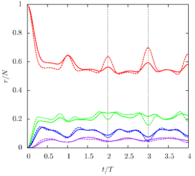
Figure 3: Occupation numbers $r/N$ of eigenmodes as a function of time in a condensate of $N=8$ (dashed lines) and $N=12$ (solid lines) particles. Initially one hole has been placed in the center and second hole at $|\xi|=1$. No full revivals are observed, and the peaks at $t=nT$ are washed out in larger system.

An $L=0$ condensate with two quasiholes is similar to an $L=N$ condensate with one quasihole, and in the thermodynamic limit the $L=N$ condensate with one vortex in the center is the ground state of the system at this angular momentum. Fig. 3 therefore suggests that in regimes $L\gtrsim N$, also a single quasihole will dephase. This seems to be reasonable, as spontaneous symmetry breaking has been predicted for states with $L\gtrsim N$ Cooper (2008); Dagnino et al. (2009a, b), and ground states in several $L$ subspaces become quasi-degenerate. That means that energy differences within each quasi-degenerate manifold are very small, while large energy jumps occur between different manifolds. Therefore, a dephasing of different contributions and thus a collapse of the quasihole must be expected. Furthermore, the smallness of energy contributions in the quasi-degenerate manifolds make revival times unobservably long. We do not further investigate this situation of $L\gtrsim N$, as the symmetry-breaking leads to the formation of vortex lattices Cooper (2008), as observed in experiments Schweikhard et al. (2004). Characteristics of the lattice should allow for a clear identification of these phases.

IV.3 Dynamics of a quasihole in the Laughlin quasiparticle state

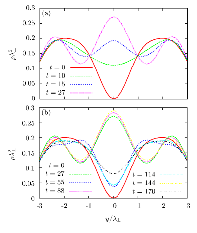
Figure 4: Density profile ($x=0$) for a system of $N=6$ particles initially prepared in the state $\hat{\mathrm{O}}_{{\rm qh}}(0)\Psi_{\rm L,qp}$ at different times $t$ (in units of $\omega_{\perp}^{-1}$) with $g=1$. In (a) the evolution from a quasihole in the center to a density peak is shown. In (b) we plot the density for all times $t<200$, at which it takes an instantaneous extremum in the center.

Upon increasing the gauge field strength, the vortex lattice has been predicted to melt when reaching filling factors $\nu\lesssim 6$ Cooper et al. (2001). Then, a variety of strongly correlated quantum liquid phases are candidates for the ground state. Finally, for $\nu=1/2$ or $L=N(N-1)$, the Laughlin state becomes the ground state of the system. It is certainly in this regime where observable properties to distinguish between the phases become most relevant. Let us therefore study the dynamics of a quasihole pierced in the last incompressible phase which has been predicted to occur before reaching the Laughlin state. It is characterized by $L=N(N-2)$ and by a wave function which differs from the Laughlin wave function only locally at the origin, having the form of a Laughlin quasiparticle excitation, $\Psi_{\rm L,qp}=\exp(-\sum_{i}|z_{i}|^{2}/2)\partial_{z_{1}}\dots\partial_{z_{N}}\prod_{i<j}(z_{i}-z_{j})$ Juliá-Díaz et al. (2012).

For simplicity, we will pierce the quasihole in the origin, which makes the resulting state an eigenstate of the single-particle part of ${\cal H}$, and all dynamics will exclusively be driven by ${\cal V}$. To obtain the state $\hat{\mathrm{O}}_{{\rm qh,0}}\Psi_{\rm L,qp}$ in the Fock basis, we numerically diagonalize the Hamiltonian ${\cal H}^{\prime}={\cal V}+V_{I}$ in the subspace $L=N(N-1)$. We then decompose this state in the corresponding eigenbasis of ${\cal V}$, also obtained by exact diagonalization. Several eigenstates of ${\cal V}$ will contribute, but the largest contribution comes from the Laughlin state with an overlap of 0.709 (0.717) for $N=7$ ($N=6$). Expressed in the eigenbasis of $\cal V$, we can easily perform the time evolution of $\hat{\mathrm{O}}_{{\rm qh}}(0)\Psi_{\rm L,qp}$.

The dynamics is clearly visible in the density shown in Fig. 4a: In the course of time, the hole fades out, as the center of the cloud gains a finite density. At some point, even a density maximum is developed at the origin, surrounded by a circular density valley. As the valley spreads out, the maximum becomes clearly peaked. The process is then reversed, and a hole at the center re-appears. Such oscillations between a density maximum and a density minimum in the center can be observed repeatedly. The scenario, however, differs from the collapse-and-revival process in the condensate: First, re-appearing holes are not equivalent to the original hole, as their density at the center remains finite, and their core size has decreased, see Fig. 4b. Second, the “revival” periods are not sharp. In Fig. 4b, we have chosen precisely those times at which the process is reversed. For $N=6$, the reversal after the first re-appearance of the quasihole is found at $t=55$, while the second revival takes place at $t=114$.

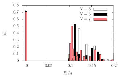
Figure 5: Overlap $c_{i}$ between $\hat{\mathrm{O}}_{{\rm qh}}(0)\Psi_{\rm L,qp}$ and eigenstates of $\cal V$ with energy $E_{i}$ for different $N$.

To understand this behavior, we have to analyze the spectrum of $\cal V$ at $L=N(N-2)+N=N(N-1)$. It can be divided into a quasi-continuous excitation band and the Laughlin state. A gap $\Delta$ separates these two contributions. For $N\gtrsim 6$, the gap approaches the constant value of $\Delta\approx 0.1g$, if we choose $g$ (rather than $gN$) to be constant Regnault and Jolicoeur (2003); Juliá-Díaz et al. (2012). Compared to this value, the energy differences between states within the excited band are typically very small. This property of the spectrum can be seen in Fig. 5, where we have plotted the overlap of the eigenstates with the initial state, $c_{i}\equiv\langle\hat{\mathrm{O}}_{{\rm qh}}(0)\Psi_{\rm L,qp}|\chi_{i}\rangle$, versus $E_{i}/g$. Here, $\left|\chi_{i}\right\rangle$ denotes the eigenstates of $\cal V$ in the $L=N(N-1)$ subspace, and $E_{i}$ is the corresponding eigenenergy.

Due to this structure, the relative dephasing of different contributions to $\hat{\mathrm{O}}_{{\rm qh}}(0)\Psi_{\rm L,qp}$ from the excited band is slow compared to the dephasing of these contributions with respect to the contribution from the Laughlin state. Following this reasoning, $2\pi/\Delta\approx 63$ for $g=1$ sets the rough time scale for a “quasi”-revival, at which the Laughlin state is again “in phase” with the low-energy contributions from the excited band. This slightly differs from the number we find by analyzing the density (cf. Fig. 4b), $t=55$ for $N=6$. But we note that the most important contribution from the excited band is a state with energy $E=0.112g$ (cf. Fig 5). Thus, it is in phase with the Laughlin after a time $t=56$. It has an overlap with $\hat{\mathrm{O}}_{{\rm qh}}(0)\Psi_{\rm L,qp}$ of 0.533. A superposition of this state and the Laughlin state is able to reproduce the quasihole state with a fidelity of 78%. Other important states, with overlaps 0.279 and 0.110, are found at $E=0.105g$ and $E=0.102g$. At $t=56$ they are still nearly in phase with the $E=0.112g$ state. But also states with $E=0.164g$ and $E=0.182g$ contribute significantly with overlaps 0.180 and 0.133. These states will be clearly out of phase, making the revival imperfect. Subsequent revivals will more and more suffer from the slow dephasing within the manifold of excited states. This explains the small irregularity in the revival periods and the loss of the quasihole character in the density profiles (see Fig. 4b).

Posing the question whether the described dynamics will survive in the thermodynamic, we first note that due to the similarity between the Laughlin state and $\hat{\mathrm{O}}_{{\rm qh}}(0)\Psi_{\rm L,qp}$, we can always expect contributions from both the Laughlin state and the excited band. This assessment seems to agree with Fig. 5, where the overlap with the Laughlin state is found to be almost constant while varying particle number, $5\leq N\leq 7$. As the Laughlin gap is known to be constant for large $N$, also the revival time has to be. The imperfection of the revival, characterized by a finite density at the center, continuously improves, as we increase the system size from $N=4$ to $N=7$. This seems reasonable, since energy differences in the excited band decrease with larger $N$, slowing down the dephasing in the excited band. In Fig. 5 this reflects in the decreased spreading of relevant states when increasing particle number. However, whether this might lead to a perfect collapse-and-revival process in the thermodynamic limit, is not clear from our calculations.

V Conclusions

We have shown that observing the dynamics of a quasihole might serve to classify different ground states in the LLL regime. Especially, the absence of decoherence is a characteristic feature of the Laughlin regime, $L\geq N(N-1)$, due to its zero interaction energy. It is in clear contrast to the collapse of the quasihole observed in finite systems with $L<N(N-1)$. For simplicity, we have considered an idealized system with a cylindrically-symmetric Hamiltonian. We note however that even deformed Laughlin states, as expected in laser-induced gauge fields Juliá-Díaz et al. (2011, 2012), should be characterized by a decoherence-free quasihole dynamics due to their vanishing interaction energy. In the condensed regime, the collapse of the quasihole is followed by a perfect revival, and the system oscillates between a condensed and a correlated state. System parameters like $gN$ and $\eta$, specifying the interaction and the single-particle energy, can be obtained by measuring period and positions of this revival. A collapse-and-revival is also found for a quasihole in the Laughlin-quasiparticle state, being an incompressible phase in the direct vicinity of the Laughlin phase.

References

- Laughlin (1983) R. B. Laughlin, Phys. Rev. Lett. 50, 1395 (1983).
- Arovas et al. (1984) D. Arovas, J. R. Schrieffer, and F. Wilczek, Phys. Rev. Lett. 53, 722 (1984).
- Cooper et al. (2001) N. R. Cooper, N. K. Wilkin, and J. M. F. Gunn, Phys. Rev. Lett. 87, 120405 (2001).
- Paredes et al. (2001) B. Paredes, P. Fedichev, J. I. Cirac, and P. Zoller, Phys. Rev. Lett. 87, 010402 (2001).
- Nayak et al. (2008) C. Nayak, S. H. Simon, A. Stern, M. Freedman, and S. Das Sarma, Rev. Mod. Phys. 80, 1083 (2008).
- Schweikhard et al. (2004) V. Schweikhard, I. Coddington, P. Engels, V. P. Mogendorff, and E. A. Cornell, Phys. Rev. Lett. 92, 040404 (2004).
- Cooper (2008) N. Cooper, Adv. Phys. 57, 539 (2008).
- Smith and Wilkin (2000) R. A. Smith and N. K. Wilkin, Phys. Rev. A 62, 061602 (2000).
- Juliá-Díaz et al. (2012) B. Juliá-Díaz, T. Graß, N. Barberán, and M. Lewenstein, New J. Phys. 14, 055003 (2012).
- Dalibard et al. (2011) J. Dalibard, F. Gerbier, G. Juzeliūnas, and P. Öhberg, Rev. Mod. Phys. 83, 1523 (2011).
- Lin et al. (2009) Y.-J. Lin, R. L. Compton, K. Jiménez-García, J. V. Porto, and I. B. Spielman, Nature 462, 628 (2009).
- Juliá-Díaz et al. (2011) B. Juliá-Díaz, D. Dagnino, K. J. Günter, T. Graß, N. Barberán, M. Lewenstein, and J. Dalibard, Phys. Rev. A 84, 053605 (2011).
- Gemelke et al. (2010) N. Gemelke, E. Sarajilic, and S. Chu, arXiv:1007.2677 (2010).
- Eberly et al. (1980) J. H. Eberly, N. B. Narozhny, and J. J. Sanchez-Mondragon, Phys. Rev. Lett. 44, 1323 (1980).
- Averbukh (1992) I. S. Averbukh, Phys. Rev. A 46, R2205 (1992).
- Rempe et al. (1987) G. Rempe, H. Walther, and N. Klein, Phys. Rev. Lett. 58, 353 (1987).
- Yeazell et al. (1990) J. A. Yeazell, M. Mallalieu, and C. R. Stroud, Phys. Rev. Lett. 64, 2007 (1990).
- Brune et al. (1996) M. Brune, F. Schmidt-Kaler, A. Maali, J. Dreyer, E. Hagley, J. M. Raimond, and S. Haroche, Phys. Rev. Lett. 76, 1800 (1996).
- Meekhof et al. (1996) D. M. Meekhof, C. Monroe, B. E. King, W. M. Itano, and D. J. Wineland, Phys. Rev. Lett. 76, 1796 (1996).
- Lewenstein and You (1996) M. Lewenstein and L. You, Phys. Rev. Lett. 77, 3489 (1996).
- Wright et al. (1996) E. M. Wright, D. F. Walls, and J. C. Garrison, Phys. Rev. Lett. 77, 2158 (1996).
- Imamoḡlu et al. (1997) A. Imamoḡlu, M. Lewenstein, and L. You, Phys. Rev. Lett. 78, 2511 (1997).
- Sørensen et al. (2001) A. Sørensen, L. M. Duan, J. I. Cirac, and P. Zoller, Nature 409, 63 (2001).
- Juliá-Díaz et al. (2012) B. Juliá-Díaz, T. Zibold, M. K. Oberthaler, M. Melé-Messeguer, J. Martorell, and A. Polls, Phys. Rev. A 86, 023615 (2012).
- Castin and Dalibard (1997) Y. Castin and J. Dalibard, Phys. Rev. A 55, 4330 (1997).
- Wright et al. (1997) E. M. Wright, T. Wong, M. J. Collett, S. M. Tan, and D. F. Walls, Phys. Rev. A 56, 591 (1997).
- Greiner et al. (2002) M. Greiner, O. Mandel, T. Hänsch, and I. Bloch, Nature 419, 51 (2002).
- Will et al. (2010) S. Will, T. Best, U. Schneider, L. Hackermüller, D.-S. Lühmann, and I. Bloch, Nature 465, 197 (2010).
- Moore and Read (1991) G. Moore and N. Read, Nucl. Phys. B 360, 362 (1991).
- Hu et al. (2012) Z.-X. Hu, K. H. Lee, and X. Wan, arXiv:1201.2105 (2012).
- Graß (2012) T. Graß, Ultracold Atoms in Artificial Gauge Fields (PhD Thesis submitted at Universitat Politècnica de Catalunya, 2012).
- Bertsch and Papenbrock (1999) G. F. Bertsch and T. Papenbrock, Phys. Rev. Lett. 83, 5412 (1999).
- Jackson and Kavoulakis (2000) A. D. Jackson and G. M. Kavoulakis, Phys. Rev. Lett. 85, 2854 (2000).
- Ueda and Nakajima (2006) M. Ueda and T. Nakajima, Phys. Rev. A 73, 043603 (2006).
- Cooper and Wilkin (1999) N. R. Cooper and N. K. Wilkin, Phys. Rev. B 60, R16279 (1999).
- Dagnino et al. (2009a) D. Dagnino, N. Barberán, M. Lewenstein, and J. Dalibard, Nature Phys. 5, 431 (2009a).
- Dagnino et al. (2009b) D. Dagnino, N. Barberán, and M. Lewenstein, Phys. Rev. A 80, 053611 (2009b).
- Regnault and Jolicoeur (2003) N. Regnault and T. Jolicoeur, Phys. Rev. Lett. 91, 030402 (2003).