Risk-Sensitive Mean Field Games

Abstract

In this paper, we study a class of risk-sensitive mean-field stochastic differential games. We show that under appropriate regularity conditions, the mean-field value of the stochastic differential game with exponentiated integral cost functional coincides with the value function described by a Hamilton-Jacobi-Bellman (HJB) equation with an additional quadratic term. We provide an explicit solution of the mean-field best response when the instantaneous cost functions are log-quadratic and the state dynamics are affine in the control. An equivalent mean-field risk-neutral problem is formulated and the corresponding mean-field equilibria are characterized in terms of backward-forward macroscopic McKean-Vlasov equations, Fokker-Planck-Kolmogorov equations, and HJB equations. We provide numerical examples on the mean field behavior to illustrate both linear and McKean-Vlasov dynamics.

I Introduction

Most formulations of mean-field (MF) models such as anonymous sequential population games [19, 7], MF stochastic controls [17, 15, 36], MF optimization, MF teams [33], MF stochastic games [34, 1, 33, 31], MF stochastic difference games [14], and MF stochastic differential games [23, 13, 32] have been of risk-neutral type where the cost (or payoff, utility) functions to be minimized (or to be maximized) are the expected values of stage-additive loss functions.

Not all behavior, however, can be captured by risk-neutral cost functions. One way of capturing risk-seeking or risk-averse behavior is by exponentiating loss functions before expectation (see [2, 18] and the references therein).

The particular risk-sensitive mean-field stochastic differential game that we consider in this paper involves an exponential term in the stochastic long-term cost function. This approach was first taken by Jacobson in [18], when considering the risk-sensitive Linear-Quadratic-Gaussian (LQG) problem with state feedback. Jacobson demonstrated a link between the exponential cost criterion and deterministic linear-quadratic differential games. He showed that the risk-sensitive approach provides a method for varying the robustness of the controller and noted that in the case of no risk, or risk-neutral case, the well known LQR solution would result (see, for follow-up work on risk-sensitive stochastic control problems with noisy state measurements, [35, 6, 27]).

In this paper, we examine the risk-sensitive stochastic differential game in a regime of large population of players. We first present a mean-field stochastic differential game model where the players are coupled not only via their risk-sensitive cost functionals but also via their states. The main coupling term is the mean-field process, also called the occupancy process or population profile process. Each player reacts to the mean field or a subset of the mean field generated by the states of the other players in an area, and at the same time the mean field evolves according to a controlled Kolmogorov forward equation.

Our contribution can be summarized as follows. Using a particular structure of state dynamics, we derive the mean-field limit of the individual state dynamics leading to a non-linear controlled macroscopic McKean-Vlasov equation; see [21]. Combining this with a limiting risk-sensitive cost functional, we arrive at the mean-field response framework, and establish its compatibility with the density distribution using the controlled Fokker-Planck-Kolmogorov forward equation. The mean-field equilibria are characterized by coupled backward-forward equations. In general a backward-forward system may not have solution (a simple example is provided in section III-D). An explicit solution of the Hamilton-Jacobi-Bellman (HJB) equation is provided for the affine-exponentiated-Gaussian mean-field problem. An equivalent risk-neutral mean-field problem (in terms of value function) is formulated and the solution of the mean-field game problem is characterized. Finally, we provide a sufficiency condition for having at most one smooth solution to the risk-sensitive mean field system in the local sense.

The rest of the paper is organized as follows. In Section II, we present the model description. We provide an overview of the mean-field convergence result in Section II-A. In Section III, we present the risk-sensitive mean-field stochastic differential game formulation and its equivalences. In Section IV, we analyze a special class of risk-sensitive mean-field games where the state dynamics are linear and independent of the mean field. In Section V, we provide a numerical example, and section VI concludes the paper. An appendix includes proofs of two main results in the main body of the paper. We summarize some of the notations used in the paper in Table I.

TABLE I: Summary of Notations

Symbol	Meaning
$f$	drift function (finite dimensional)
$\sigma$	diffusion function (finite dimensional)
${x}^{n}_{j}(t)$	state of Player $j$ in a population of size $n$
$\bar{x}_{j}(t)$	solution of macroscopic McKean-Vlasov equation
${x}_{j}(t)$	limit of state process ${x}^{n}_{j}(t)$
$U_{j}$	space of feasible control actions of Player $j$
$\tilde{\gamma}_{j}$	state feedback strategy of Player $j$
$\bar{\gamma}_{j}$	individual state-feedback strategy of Player $j$
$\tilde{\Gamma}_{j}$	set of admissible state feedback strategies of Player $j$
$\bar{\Gamma}_{j}$	set of admissible individual state-feedback strategies of Player $j$
$u_{j}$	control action of Player $j$ under a generic control strategy
$c$	instantaneous cost function
$g$	terminal cost function
$\delta$	risk-sensitivity index
$\mathbb{B}_{j}$	standard Brownian motion process for Player $j$’s dynamics
$\mathbb{E}$	Expectation operator
$L$	risk-sensitive cost functional
$\partial_{x}$	partial derivative with respect to $x$ (gradient)
$\partial^{2}_{xx}$	second partial derivative (Hessian operator) with the respect to $x$
$x^{\prime}$	transpose of $x$
$m^{n}_{t}$	empirical measure of the states of the players
$m_{t}$	limit of $m_{t}^{n}$ when $n\rightarrow\infty$
$m^{n}$	limit of $m_{t}^{n}$ when $t\rightarrow\infty$
tr($M$)	trace of a square matrix $M$, i.e., $tr(M):=\sum_{i}M_{ii}.$
$A\succ B$	$A-B$ is positive definite, where $A$, $B$ are square symmetric matrices of the same dimension.

II The problem setting

We consider a class of $n-$person stochastic differential games, where Player $j$’s individual state, $x_{j}^{n}$, evolves according to the Itô stochastic differential equation (S) as follows:

$$\begin{array}[]{ccl}dx_{j}^{n}(t)&=&\frac{1}{n}\displaystyle\sum_{i=1}^{n}f_{ji}(t,x_{j}^{n}(t),u^{n}_{j}(t),x_{i}^{n}(t))dt+\frac{\sqrt{\epsilon}}{n}\displaystyle\sum_{i=1}^{n}\sigma_{ji}(t,x_{j}^{n}(t),u^{n}_{j}(t),x_{i}^{n}(t))d\mathbb{B}_{j}(t),\\ x_{j}^{n}(0)&=&x_{j,0}\in\mathcal{X}\subseteq\mathbb{R}^{k},\ k\geq 1,j\in\{1,\ldots,n\},\end{array}\ (\textrm{S})$$

where $x_{j}^{n}(t)$ is the $k$-dimensional state of Player $j$; $u_{j}^{n}(t)\in{U}_{j},$ is the control of Player $j$ at time $t$ with ${U}_{j}$ being a subset of the $p_{j}$-dimensional Euclidean space $\mathbb{R}^{p_{j}}$; $\mathbb{B}_{j}(t)$ are mutually independent standard Brownian motion processes in $\mathbb{R}^{k}$; and $\epsilon$ is a small positive parameter, which will play a role in the analysis in the later sections. We will assume in (S) that there is some symmetry in $f_{ji}$ and $\sigma_{ji}$, in the sense that there exist $f$ and $\sigma$ (conditions on which will be specified shortly) such that for all $j$ and $i$,

$$f_{ji}(t,x_{j}^{n}(t),u^{n}_{j}(t),x_{i}^{n}(t))\equiv f(t,x_{j}^{n}(t),u^{n}_{j}(t),x_{i}^{n}(t))$$

and

$$\sigma_{ji}(t,x_{j}^{n}(t),u^{n}_{j}(t),x_{i}^{n}(t))\equiv\sigma(t,x_{j}^{n}(t),u^{n}_{j}(t),x_{i}^{n}(t))\,.$$

The system (S) is a controlled McKean-Vlasov dynamics. Historically, the McKean-Vlasov stochastic differential equation (SDE) is a kind of mean field forward SDE suggested by Kac in 1956 as a stochastic toy model for the Vlasov kinetic equation of plasma and the study of which was initiated by McKean in 1966. Since then, many authors have made contributions to McKean-Vlasov type SDEs and related applications [20, 10].

The uncontrolled version of state dynamics (S) captures many interesting problems involving interactions between agents. We list below a few examples.

Example 1 (Stochastic Kuramoto model).

Consider $n$ oscillators where each of the oscillators is considered to have its own intrinsic natural frequency $\omega_{j}$, and each is coupled symmetrically to all other oscillators. For $f_{ji}(x_{i},u_{i},x_{j})=f(x_{i},u_{i},x_{j})=K\sin(x_{j}-x_{i})+\omega_{j}$ and $\sigma_{ji}$ a constant in (S), the state dynamics without control is known as (stochastic) Kuramoto oscillator [22] where the goal is convergence to some common value (consensus) or alignment of the players’ parameters. The stochastic Kuramoto model is given by

$${d\theta_{j}}(t)=\left(\omega_{j}(t)+\dfrac{K}{n}\sum_{i=1}^{n}\sin(\theta_{i}(t)-\theta_{j}(t))\right)dt+Dd\mathbb{B}_{j}(t),$$

where $D,K>0.$

Example 2 (Stochastic Cucker-Smale dynamics:).

Consider a population, say of birds or fish that move in the three dimensional space. It has been observed that for some initial conditions, for example on their positions and velocities, the state of the flock converges to one in which all birds fly with the same velocity. See, for example, Cucker-Smale flocking dynamics [9, 8] where each vector $x_{i}=(y_{i},v_{i})$ is composed of position dynamics and velocity dynamics of the corresponding player. For $f(x_{i},u_{i},x_{j})=(\epsilon^{2}+\parallel x_{j}-x_{i}\parallel^{2})^{-\alpha}c(x_{j}-x_{i})$ in (S), where $\epsilon>0,\alpha>0$ and $c(\cdot)$ is a continuous function, one arrives at a generic class of consensus algorithms developed for flocking problems.

Example 3 (Temperature dynamics for energy-efficient buildings).

Consider a heating system serving a finite number of zones. In each zone, the goal is to maintain a certain temperature. Denote by $T_{j}$ the temperature of zone $j,$ and by $T^{ext}$ the ambient temperature. The law of conservation of energy can be written down as the following equation for zone $j,$

$$dT_{j}(t)=\sigma d\mathbb{B}_{j}(t)+\left[r_{j}(t)+\frac{\gamma}{\beta}(T^{ext}(t)-T_{j}(t))+\sum_{i\neq j}\alpha_{ij}(t)(T_{i}(t)-T_{j}(t))\right]dt,$$

where $r_{j}$ denotes the heat input rate of the heater in zone $j,$ $\gamma,\beta>0,$ $\alpha_{ij}$ is the thermal conductance between zone $i$ and zone $j$ and $\sigma$ is a small variance term. The evolution of the temperature has a McKean-Vlasov structure of the type in system (S). We can introduce a control variable into $r_{j}$ such that the heater can be turned on and off in each zone.

The three examples above can be viewed as special cases of the system (S). The controlled dynamics in (S) allows one to address several interesting questions. For example, how to control the flocking dynamics and consensus algorithms of the first two examples above to a certain target? How to control the temperature in the third example in order to achieve a specific thermal comfort while minimizing energy cost? In order to define the controlled dynamical system in precise terms, we have to specify the nature of information that players are allowed in the choice of their control at each point in time. This brings us to the first definition below.

Definition 1.

A state-feedback strategy for Player $j$ is a mapping $\tilde{\gamma}_{j}:\ \mathbb{R}_{+}\times(\mathbb{R}^{k})^{n}\longrightarrow{U}_{j}$, whereas an individual state-feedback strategy for Player $j$ is a mapping $\bar{\gamma}_{j}:\ \mathbb{R}_{+}\times\mathbb{R}^{k}\longrightarrow{U}_{j}.$

Note that the individual state-feedback strategy involves only the self state of a player, whereas the state-feedback strategy involves the entire $nk-$dimensional state vector. The individual strategy spaces in each case have to be chosen in such a way that the resulting system of stochastic differential equations (S) admits a unique solution (in the sense specified shortly) when the players pick their strategies independently; furthermore, the feasible sets are time invariant and independent of the controls. We denote by $\bar{\Gamma}_{j}$ the set of such admissible control laws $\bar{\gamma}_{j}:[0,T]\times\mathbb{R}^{k}\rightarrow{U}_{j}$ for Player $j$; a similar set, $\tilde{\Gamma}_{j}$, can be defined for state-feedback strategies $\tilde{\gamma}_{j}$.

We assume the following standard conditions on $f,\sigma,\bar{\gamma}_{j}$ and the action sets $U_{j}$, for all $j=1,2,\cdots,n$.

• $f$ is $C^{1}$ in $(t,x,u,m)$, and Lipschitz in $(x,u,m)$.

• The entries of the matrix $\sigma$ are $C^{2}$ and $\sigma\sigma^{\prime}$ is strictly positive;

• $f,\partial_{x}f$ are uniformly bounded;

• ${U}_{j}$ is non-empty, closed and bounded;

• $\bar{\gamma}_{j}:\ [0,T]\times\mathbb{R}^{k}\longrightarrow{U}_{j}$ is piecewise continuous in $t$ and Lipschitz in $x.$

Normally, when we have a cost function for Player $j$, which depends also on the state variables of the other players, either directly, or implicitly through the coupling of the state dynamics (as in (S)), then any state-feedback Nash equilibrium solution will generally depend not only on self states but also on the other states, i.e., it will not be in the set $\bar{\Gamma}_{j},j=1,\cdots,n$. However, this paper aims to characterize the solution in the high-population regime (i.e., as $n\rightarrow\infty$) in which case the dependence on other players’ states will be through the distribution of the player states. Hence each player will respond (in an optimal, cost minimizing manner) to the behavior of the mass population and not to behaviors of individual players. Validity of this property will be established later in Section III of the paper, but in anticipation of this, we first introduce the quantity

$$m^{n}_{t}=\frac{1}{n}\sum_{j=1}^{n}\delta_{x_{j}^{n}(t)},$$ (1)

as an empirical measure of the collection of states of the players, where $\delta$ is a Dirac measure on the state space. This enables us to introduce the long-term cost function of Player $j$ (to be minimized by him) in terms of only the self variables ($x_{j}$ and $u_{j}$) and $m_{t}^{n},t\geq 0$, where the latter can be viewed as an exogenous process (not directly influenced by Player $j$). But we first introduce a mean-field representation of the dynamics (S), which uses $m^{n}_{t}$ and will be used in the description of the cost.

II-A Mean-field representation

The system (S) can be written into a measure representation using the formula

$$\int\phi(w)\left[\sum_{i=1}^{n}\bar{\omega}_{i}\delta_{x_{i}}\right](dw)=\sum_{i=1}^{n}\bar{\omega}_{i}\phi(x_{i}),$$

where $\delta_{z},z\in\mathcal{X}$ is a Dirac measure concentrated at $z$, $\phi$ is a measurable bounded function defined on the state space and $\bar{\omega}_{i}\in\mathbb{R}$. Then, the system (S) reduces to the system

$$dx_{j}^{n}(t) = \left(\int_{w}f(t,x_{j}^{n}(t),u^{n}_{j}(t),w)\left[\frac{1}{n}\sum_{i=1}^{n}\delta_{x_{i}^{n}(t)}\right](dw)\right)dt$$

$$+ \sqrt{\epsilon}\left(\int_{w}\sigma(t,x_{j}^{n}(t),u^{n}_{j}(t),w)\left[\frac{1}{n}\sum_{i=1}^{n}\delta_{x_{i}^{n}(t)}\right](dw)\right)d\mathbb{B}_{j}(t),$$

$$x_{j}^{n}(0) = x_{j,0}\in\mathbb{R}^{k},\ k\geq 1,j\in\{1,\ldots,n\},$$

which, by (1), is equivalent to the following system (SM):

$$\begin{array}[]{lll}\displaystyle dx_{j}^{n}(t)&=&\left(\displaystyle\int_{w}f(t,x_{j}^{n}(t),u^{n}_{j}(t),w)m^{n}_{t}(dw)\right)dt\\ &&+\sqrt{\epsilon}\left(\displaystyle\int_{w}\sigma(t,x_{j}^{n}(t),u^{n}_{j}(t),w)m^{n}_{t}(dw)\right)d\mathbb{B}_{j}(t),\\ x_{j}^{n}(0)&=&x_{j,0}\in\mathbb{R}^{k},\ k\geq 1,j\in\{1,\ldots,n\}.\end{array}$$

The above representation of the system (SM) can be seen as a controlled interacting particles representation of a macroscopic McKean-Vlasov equation where $m^{n}_{t}$ represents the discrete density of the population. Next, we address the mean field convergence of the population profile process $m^{n}.$ To do so, we introduce the key notion of indistinguishability.

Definition 2 (Indistinguishability).

We say that a family of processes $(x^{n}_{1},x^{n}_{2},\ldots,x^{n}_{n})$ is indistinguishable (or exchangeable) if the law of $x^{n}$ is invariant by permutation over the index set $\{1,\ldots,n\}.$

The solution of (S) obtained under fixed control $u(\cdot)$ generates indistinguishable processes. For any permutation $\pi$ over $\{1,2,\ldots,n\}$, one has $\mathcal{L}(x^{n}_{j_{1}},\ldots,x^{n}_{j_{n}})=\mathcal{L}(x^{n}_{\pi(j_{1})},\ldots,x^{n}_{\pi(j_{n})}),\$ where $\mathcal{L}(X)$ denotes the law of the random variable $X.$ For indistinguishable (exchangeable) processes, the convergence of the empirical measure has been widely studied (see [29] and the references therein). To preserve this property for the controlled system we restrict ourselves to admissible homogeneous controls. Then, the mean field convergence is equivalent to the existence of a random measure $\mu$ such that the system is $\mu-$chaotic, i.e.,

$$\lim_{n}\int\prod_{l=1}^{L}\phi_{l}({x}^{n}_{j_{l}})\mu^{n}(dx^{n})=\prod_{l=1}^{L}\left(\int\phi_{l}d\mu\right),$$

for any fixed natural number $L\geq 2$ and a collection of measurable bounded functions $\{\phi_{l}\}_{1\leq l\leq L}$ defined over the state space $\mathcal{X}.$ Following the indistinguishability property, one has that the law of $x^{n}_{j}=(x_{j}^{n}(t),\ t\geq 0)$ is $\mathbb{E}[m^{n}].$ The same result is obtained by proving the weak convergence of the individual state dynamics to a macroscopic McKean-Vlasov equation (see later Proposition 5). Then, when the initial states are i.i.d. and given some homogeneous control actions $u,$ the solution of the state dynamics generates an indistinguishable random process and the weak convergence of the population profile process $m^{n}$ to $\mu$ is equivalent to the $\mu-$chaoticity. For general results on mean-field convergence of controlled stochastic differential equations, we refer to [14]. These processes depend implicitly on the strategies used by the players. Note that an admissible control law $\bar{\gamma}$ may depend on time $t$, the value of the individual state $x_{j}(t)$ and the mean-field process $m_{t}$. The weak convergence of the process $m^{n}$ implies the weak convergence of its marginal $m^{n}_{t}$ and one can characterize the distribution of $m_{t}$ by the Fokker-Planck-Kolmogorov (FPK) equation:

$\partial_{t}m_{t}+D^{1}_{x}\left(m_{t}\displaystyle\int_{w}f(t,x,u(t),w)m_{t}(dw)\right)$

$$= \frac{\epsilon}{2}D^{2}_{xx}\left(m_{t}\left(\int_{w}\sigma^{\prime}(t,x,u(t),w)m_{t}(dw)\right)\cdot\left(\int_{w}\sigma(t,x,u(t),w)m_{t}(dw)\right)\right).$$ (2)

Here $f(\cdot)\in\mathbb{R}^{k},$ which we denote by $(f_{k^{\prime}}(\cdot))_{1\leq k^{\prime}\leq k},$ where $f_{k^{\prime}}$ is scalar. We let

$$\underline{\sigma}[t,x,u(t),m_{t}]:=\int_{w}\sigma(t,x,u(t),w)m_{t}(dw),$$

$\Gamma(\cdot):=\underline{\sigma}(\cdot)\underline{\sigma}^{\prime}(\cdot)$ is a square matrix with dimension $k\times k.$ The term $D^{1}_{x}(\cdot)$ denotes

$$\sum_{k^{\prime}=1}^{k}\frac{\partial}{\partial x_{k^{\prime}}}\left(m_{t}\int_{w}f_{k^{\prime}}(t,x,u(t),w)m_{t}(dw)\right),$$

and the last term on $D^{2}_{xx}(\cdot)$ is

$$\sum_{k^{\prime\prime}=1}^{k}\sum_{k^{\prime}=1}^{k}\frac{\partial^{2}}{\partial x_{k^{\prime}}\partial x_{k^{\prime\prime}}}\left(m_{t}\Gamma_{k^{\prime}k^{\prime\prime}}(\cdot)\right).$$

In the one-dimensional case, the terms $D^{1},D^{2}$ reduce to the divergence “div” and the Laplacian operator $\Delta$, respectively.

It is important to note that the existence of a unique rest point (distribution) in FPK does not automatically imply that the mean-field converges to the rest point when $t$ goes to infinity. This is because the rest point may not be stable.

Remark 1.

In mathematical physics, convergence to an independent and identically distributed system is sometimes referred to as chaoticity [28, 29, 11], and the fact that chaoticity at the initial time implies chaoticity at further times is called propagation of chaos. However in our setting the chaoticity property needs to be studied together with the controls of the players. In general the chaoticity property may not hold. One particular case should be mentioned, which is when the rest point $m^{*}$ is related to the $\delta_{m^{*}}-$ chaoticity. If the mean-field dynamics has a unique global attractor $m^{*}$, then the propagation of chaos property holds for the measure $\delta_{m^{*}}.$ Beyond this particular case, one may have multiple rest points but also the double limit, $\lim_{n}\lim_{t}m^{n}_{t}$ may differ from the one when the order is swapped, $\lim_{t}\lim_{n}m^{n}_{t}$ leading a non-commutative diagram. Thus, a deep study of the underlying dynamical system is required if one wants to analyze a performance metric for a stationary regime. A counterexample of non-commutativity of the double limit is provided in [30].  

II-B Cost Function

We now introduce the cost functions for the differential game. Risk-sensitive behaviors can be captured by cost functions which exponentiate loss functions before the expectation operator. For each $t\in[0,T]$, and $m_{t}^{n},x_{j}$ initialized at a generic feasible pair $\underline{m},\underline{x}$ at $t$, the risk-sensitive cost function for Player $j$ is given by

$$L(\bar{\gamma}_{j},m^{n}_{[t,T]};t,\underline{x},\underline{m})=\delta\log\mathbb{E}\left(e^{\frac{1}{\delta}[\displaystyle g(x_{T})+\int_{t}^{T}c(s,x_{j}^{n}(s),u_{j}^{n}(s),m^{n}(s))\ ds]}\ \Bigg{|}\ x_{j}(t)=\underline{x},m^{n}_{t}=\underline{m}\right),$$ (3)

where $c(\cdot)$ is the instantaneous cost at time $s$; $g(\cdot)$ is the terminal cost; $\delta>0$ is the risk-sensitivity index; $m^{n}_{[t,T]}$ denotes the process $\{m^{n}_{s},t\leq s\leq T\}$; and $u_{j}^{n}(s)=\bar{\gamma}_{j}(s,x_{j}^{n}(s),m^{n}(s)),$ with $\bar{\gamma}_{j}\in\bar{\Gamma}_{j}$. Note that because of the symmetry assumption across players, the cost function of Player $j$ is not indexed by $j$, since it is in the same structural form for all players. This is still a game problem (and not a team problem), however, because each such cost function depends only on the self variables (indexed by $j$ for Player $j$) as well as the common population variable $m^{n}$.

We assume the following standard conditions on $c$ and $g$.

• $c$ is $C^{1}$ in $(t,x,u,m)$; $g$ is $C^{2}$ in $x$; $c,g$ are non-negative;

• $c,\partial_{x}c,g,\partial_{x}g$ are uniformly bounded.

The cost function (3) is called the risk-sensitive cost functional or the exponentiated integral cost, which measures risk-sensitivity for the long-run and not at each instant of time (see [18, 35, 6, 2]). We note that the McKean-Vlasov mean field game considered here differs from the model in [16]; specifically, in this paper, the volatility term in (SM) is a function of state, control and the mean field, and further, the cost functional is of the risk-sensitive type.

Remark 2 (Connection with mean-variance cost).

Consider the function $c^{\lambda}:\ \lambda\longmapsto\frac{1}{\lambda}\log(\mathbb{E}e^{\lambda C}).$ It is obvious that the risk-sensitive cost $c^{\lambda}$ takes into consideration all the moments of the cost $C$, and not only its mean value. Around zero, the Taylor expansion of $c^{\lambda}$ is given by

$$c^{\lambda}\underbrace{\approx}_{\lambda\sim 0}\mathbb{E}(C)+\frac{\lambda}{2}\textrm{var}(C)+o(\lambda),$$

where the important terms are the mean cost and the variance of the cost for small $\lambda.$ Hence risk-sensitive cost entails a weighted sum of the mean and variance of the cost, to some level of approximation.

With the dynamics (SM) and cost functionals as introduced, we seek an individual state-feedback non-cooperative Nash equilibrium $\{\bar{\gamma}^{*}_{i},i\in\{1,\cdots,n\}\}$, satisfying the set of inequalities

$$L(\bar{\gamma}^{*}_{j},m^{n}_{[0,T]};0,x_{j,0},\underline{m})\leq L(\bar{\gamma}_{j},\tilde{m}^{n,j}_{[0,T]};0,x_{j,0},\underline{m}),$$ (4)

for all $\bar{\gamma}_{j}\in\bar{\Gamma}_{j},j\in\{1,2,\cdots,n\}$, where $m^{n}[0,T]$ is generated by the $\bar{\gamma}_{j}^{*}$’s, and $\tilde{m}^{n,j}_{[0,T]}$ by $(\bar{\gamma},\bar{\gamma}_{-j}^{*})$, $\bar{\gamma}_{-j}^{*}=\{\bar{\gamma}_{i}^{*},i=1,2,\cdots,n,i\neq j\}$; $u^{*}_{j}$ and $u_{j}$ are control actions generated by control laws $\bar{\gamma}^{*}_{j}$ and $\bar{\gamma}_{j}$, respectively, i.e., $u^{*}_{j}=\bar{\gamma}^{*}_{j}(t,x_{j})$ and $u_{j}=\bar{\gamma}_{j}(t,x_{j})$; $m^{n}_{t}=m^{n}_{t}[u^{*}]$ laws are given by forward FPK equation under the strategy $\bar{\gamma}^{*},$ and $\tilde{m}^{n,j}_{t}=\tilde{m}^{n,j}_{t}[u_{j},u_{-j}^{*}]$ is the induced measure under the strategy $(\bar{\gamma}_{j},\bar{\gamma}_{-j}^{*}).$

A more stringent equilibrium solution concept is that of strongly time-consistent individual state-feedback Nash equilibrium satisfying,

$$L(\bar{\gamma}^{*}_{j},m^{n}_{[t,T]};t,x_{j},\underline{m})\leq L(\bar{\gamma}_{j},\tilde{m}^{n,j}_{[t,T]};t,x_{j},\underline{m}),$$ (5)

for all $x_{j}\in\mathcal{X}$, $t\in[0,T)$, $\bar{\gamma}_{j}\in\bar{\Gamma}_{j},j\in\{1,2,\cdots,n\}.$

Note that the two measures $m^{n}_{t}$ and $\tilde{m}^{n,j}_{t}$ differ only in the component $j$ and have a common term which is $\frac{1}{n}\sum_{j^{\prime}\neq j}\delta_{x^{n}_{j^{\prime}}(t)}$, which converges in distribution to some measure with a distribution that is a solution of the forward PFK partial differential equation.

III Risk-sensitive best response to mean-field and equilibria

In this section, we present the risk-sensitive mean-field results. We first provide an overview of the mean-field (feedback) best response for a given mean-field trajectory $m^{n}=(m^{n}(s),\ s\geq 0).$ A mean-field best-response strategy of a generic Player $j$ to a given mean field $m_{t}^{n}$ is a measurable mapping $\bar{\gamma}^{*}_{j}$ satisfying: $\ \forall\ \bar{\gamma}_{j}\in\bar{{\Gamma}}_{j}$, with $x_{j}$ and $m^{n}_{t}$ initialized at $x_{j,0},\underline{m}$, respectively,

$$L(\bar{\gamma}_{j}^{*},m^{n}_{[0,T]},0,x_{j,0},\underline{m})\leq L(\gamma_{j},m^{n}_{[0,T]},0,x_{j,0},\underline{m}).$$

where law of $m^{n}_{t}$ is given by the forward FPK equation in the whole space $\mathcal{X}^{n}$, and is an exogenous process. Let $v^{n}(t,x_{j},\underline{m})=\inf_{u_{j}}L({u}_{j},m^{n}_{[0,T]},t,x_{j},\underline{m}).$ The next proposition establishes the risk-sensitive Hamilton-Jacobi-Bellman (HJB) equation of the risk-sensitive cost function satisfied by a smooth optimal value function of a generic player. The main difference from the standard HJB equation is the presence of the term $\frac{\epsilon}{2\delta}\parallel\sigma\partial_{x_{j}}v^{n}\parallel^{2}.$

Proposition 1.

Suppose that the trajectory of $m^{n}_{t}$ is given. If $v^{n}$ is twice continuously differentiable, then $v^{n}$ is solution of the risk-sensitive HJB equation

$$\partial_{t}v^{n}+\inf_{u_{j}}\left\{f\cdot\partial_{x_{j}}v^{n}+\frac{\epsilon}{2}{tr}(\sigma\sigma^{\prime}\partial^{2}_{x_{j}x_{j}}v^{n}_{j})+\frac{\epsilon}{2\delta}\parallel\sigma\partial_{x_{j}}v^{n}\parallel^{2}+c\right\} = 0,$$

$$v^{n}(T,x_{j}) = g(x_{j}).$$

Moreover, any strategy satisfying

$$\bar{\gamma}^{n}_{j}(\cdot)\in\arg\min_{u_{j}}\left\{f\cdot\partial_{x_{j}}v^{n}+\frac{\epsilon}{2}{tr}(\sigma\sigma^{\prime}\partial^{2}_{x_{j}x_{j}}v^{n})+\frac{\epsilon}{2\delta}\parallel\sigma\partial_{x_{j}}v^{n}\parallel^{2}+c\right\},$$

constitutes a best response strategy to the mean-field $m^{n}.$

Proof of Proposition 1.

For feasible initial conditions $\underline{x}$ and $\underline{m}$, we define

$$\phi^{n}(t,\underline{x},\underline{m}):=\inf_{{u}^{n}_{j}}\mathbb{E}\left(e^{\frac{1}{\delta}[g(x_{T})+\int_{t}^{T}c(s,x^{n}(s),u_{j}(t),m^{n}_{s})\ ds]}\ |\ x_{j}(t)=\underline{x},m^{n}_{t}=\underline{m}\right).$$

It is clear that $v^{n}(t,x_{j},\underline{m})=\inf L=\delta\log\phi^{n}(t,x_{j},\underline{m}).$ Under the regularity assumptions of Section II, the function $\phi^{n}$ is $C^{1}$ in $t$ and $C^{2}$ in $x.$ Using Itô’s formula,

$$d\phi^{n}(t,x_{j})=[\partial_{t}\phi^{n}(t,x_{j})+f\cdot\partial_{x_{j}}\phi^{n}+\frac{\epsilon}{2}\textrm{tr}(\sigma\sigma^{\prime}\partial^{2}_{x_{j}x_{j}}\phi^{n})]dt.$$

Using the Ito-Dynkin’s formula (see [26, 6, 27]), the dynamic optimization yields

$$\inf_{\bar{u}_{j}}\{d\phi^{n}+\frac{1}{\delta}c\phi^{n}dt\}=0.$$

Thus, one obtains

$$\partial_{t}\phi^{n}+\inf_{u_{j}}\left\{f\cdot\partial_{x_{j}}\phi^{n}+\frac{\epsilon}{2}\textrm{tr}(\sigma\sigma^{\prime}\partial^{2}_{xx}\phi^{n})+\frac{1}{\delta}c\phi^{n}\right\} = 0,$$

$$\phi^{n}(T,x_{j}) = e^{\frac{1}{\delta}g(x_{j})}.$$

To establish the connection with the risk-sensitive cost value, we use the relation $\phi^{n}=e^{\frac{1}{\delta}v^{n}}$. One can compute the partial derivatives:

$$\partial_{t}\phi^{n}=\left(\partial_{t}v^{n}\right)\frac{1}{\delta}\phi^{n},\ \ \partial_{x_{j}}\phi^{n}=\left(\partial_{x_{j}}v^{n}\right)\frac{1}{\delta}\phi^{n},$$

and

$$\partial^{2}_{x_{j}x_{j}}\phi^{n}=\left(\partial^{2}_{x_{j}x_{j}}v^{n}\right)\frac{1}{\delta}\phi^{n}+\frac{1}{\delta^{2}}\left(\partial_{x_{j}}v^{n}\right)^{\prime}\left(\partial_{x_{j}}v^{n}\right)\phi^{n},$$

where the latter immediately yields

$$\textrm{tr}(\partial^{2}_{x_{j}x_{j}}\phi^{n}\sigma\sigma^{\prime})=\textrm{tr}(\partial^{2}_{x_{j}x_{j}}v^{n}\sigma\sigma^{\prime})\frac{1}{\delta}\phi^{n}+\frac{1}{\delta^{2}}\parallel\sigma\partial_{x_{j}}v^{n}\parallel^{2}\phi^{n}.$$

Combining together and dividing by $\phi^{n}/\delta,$ we arrive at the HJB equation (1).

∎

Remark 3.

Let us introduce the Hamiltonian $H$ as

$$H(t,x,\tilde{p},\tilde{M})=\inf_{u}\left\{\tilde{p}\cdot f+\frac{\epsilon}{2}{tr}(\sigma\sigma^{\prime}\tilde{M})+\frac{\epsilon}{2\delta}\parallel\sigma\tilde{p}\parallel^{2}+c\right\},$$

for a vector $\tilde{p}$ and a matrix $\tilde{M}$ which is the same as the Hessian of $v^{n}.$

If $\sigma$ does not depend on the control, then the above expression reduces to

$$\inf_{u}\{\tilde{p}\cdot f+c\}+\frac{\epsilon}{2}{tr}(\sigma\sigma^{\prime}\tilde{M})+\frac{\epsilon}{2\delta}\parallel\sigma\tilde{p}\parallel^{2},$$

and the term to be minimized is $H^{2}(t,x,\tilde{p},\tilde{M})=\inf_{u}\{\tilde{p}\cdot f+c\},$ which is related to the Legendre-Fenchel transform for linear dynamics, i.e., the case where $f$ is linear in the control $u.$

In that case,

$$\partial_{\tilde{p}}H^{2}(t,x,\tilde{p},\tilde{M})=\alpha u^{*}$$

for some non-singular $\alpha$ of proper dimension. This says that the derivative of the modified Hamiltonian is related to the optimal feedback control. Now, for non-linear drift $f$ the same technique can be used but the function $f$ needs to be inverted to obtain a generic closed form expression the optimal feedback control and is given by

$$u^{*}_{j}=\tilde{g}^{-1}(\partial_{\tilde{p}}H^{2}(t,x,\tilde{p},\tilde{M})),$$

where $\tilde{g}^{-1}$ is the inverse of the map

$$u\longmapsto f(t,x,u,m).$$

This generic expression of the optimal control will play an important role in non-linear McKean-Vlasov mean field games.

The next proposition provides the best-response control to the affine-quadratic in $u$-exponentiated cost-Gaussian mean-field game, and the proposition that follows that deals with the case of affine-quadratic in both $u$ and $x$.

Proposition 2.

Suppose $\sigma(t,x)=\sigma(t)$ and

$$f(t,x_{j},u_{j},m) = \bar{f}(t,x_{j},m)+B(t,x_{j},m)u_{j},$$

$$c(t,x_{j},u_{j},m) = \bar{c}(t,x_{j},m)+\parallel u_{j}\parallel^{2}.$$

Then, the best-response control of Player $j$ is $\bar{\gamma}_{j}^{n,*}=-\frac{1}{2}B\partial_{x_{j}}v^{n}.$

Proof.

Following Proposition 1, we know

$$\bar{u}^{n,*}_{j}=\bar{\gamma}^{n,*}_{j}(\cdot)\in\arg\min_{u_{j}}\{c(t,x_{j}(t),u_{j}(t),m_{t})+f(t,x_{j}(t),u_{j},m_{t})\cdot\partial_{x_{j}}v^{n}\}.$$

With the assumptions on $\sigma,f,c,g$, the condition reduces to

$$\arg\min_{u_{j}}\left\{[\bar{f}+Bu_{j}]\partial_{x_{j}}v^{n}+\bar{c}+\parallel u_{j}\parallel^{2}\right\}.$$

and hence, we obtain $\bar{\gamma}_{j}^{n,*}=-\frac{1}{2}B\partial_{x_{j}}v^{n}$ by convexity and coercivity of the mapping $u_{j}\longmapsto[\bar{f}+Bu_{j}]\partial_{x_{j}}v^{n}+\bar{c}+\parallel u_{j}\parallel^{2}.$ ∎

Proposition 3 (Explicit optimal control and cost, [2]).

Consider the risk-sensitive mean-field stochastic game described in Proposition 2 with $\bar{f}=A(t)x$, $B$ a constant matrix, $c=x^{\prime}Q(t)x,\ Q(t)\geq 0,\ g(x)=x^{\prime}Q_{T}x,Q_{T}\geq 0,$ where the symmetric matrix $Q(\cdot)$ is continuous. Then, the solution to HJB equation in Proposition 1 (whenever it exists) is given by $v^{n}(t,x)=x^{\prime}Z(t)x+\epsilon\int_{t}^{T}{tr}(Z(s)\sigma\sigma^{\prime})\ ds.$ where $Z(s)$ is the nonnegative definite solution of the generalized Riccati differential equation

$$\dot{Z}+A^{\prime}Z+ZA+Q-Z\left(BB^{\prime}-\frac{1}{\rho^{2}}\sigma\sigma^{\prime}\right)Z=0,\ Z(T)=Q_{T},$$

where $\rho=(\frac{\delta}{2\epsilon})^{1/2}$ and the optimal response strategy is

$$u^{*}_{j}(t)=\bar{\gamma}^{*}_{j}(\cdot)=-B^{\prime}Zx.$$ (6)

Using Proposition 3, one has the following result for any given trajectory $(m^{n}_{t})_{t\geq 0},$ which enters the cost function in a particular way.

Proposition 4.

If $c$ is in the form $c=x^{\prime}(Q(t)-\Lambda(t,m^{n}_{t}))x$, where $\Lambda$ is symmetric and continuous in $(t,m)$, then the generalized Riccati equation becomes

$$\dot{Z}^{*}+A^{\prime}Z^{*}+Z^{*}A+Q-\Lambda(t,m^{n}_{t})-Z^{*}\left(BB^{\prime}-\frac{1}{\rho^{2}}\sigma\sigma^{\prime}\right)Z^{*}=0,Z^{*}(T)=Q_{T},$$

and

$$v^{n}(t,x)=x^{\prime}Z^{*}x+\epsilon\int_{t}^{T}{tr}(Z^{*}(s)\sigma\sigma^{\prime})\ ds.$$

III-A Macroscopic McKean-Vlasov equation

Since the controls used by the players influence the mean-field limit via the state dynamics, we need to characterize the evolution of the mean-field limit as a function of the controls. The law of $m_{t}$ is the solution of the Fokker-Planck-Kolmogorov equation given by (2) and the individual state dynamics follows the so-called macroscopic McKean-Vlasov equation

$$d\bar{x}_{j}(t)=\left(\int_{w}f(t,\bar{x}_{j}(t),u_{j}^{*}(t),w)m_{t}(dw)\right)dt+\sqrt{\epsilon}\left(\int_{w}\sigma(t,\bar{x}_{j}(t),u_{j}^{*}(t),w)m_{t}(dw)\right)d\mathbb{B}_{j}(t).$$ (7)

In order to obtain an error bound, we introduce the following notion: Given two measures $\mu$ and $\nu$ the Monge-Kontorovich metric (also called Wasserstein metric) between $\mu$ and $\nu$ is

$$\mathcal{W}_{1}(\mu,\nu)=\inf_{X\sim\mu,Y\sim\nu}\mathbb{E}|X-Y|.$$

In other words, let $E(\mu,\nu)$ be the set of probability measures $\mathbb{P}$ on the product space such that the image of $\mathbb{P}$ under the projection on the first argument (resp. on the second argument) is $\mu$ (resp. $\nu$). Then,

$$\mathcal{W}_{1}(\mu,\nu)=\inf_{\mathbb{P}\in E(\mu,\nu)}\int\int|z-z^{\prime}|\mathbb{P}(dz,dz^{\prime}).$$ (8)

This is known indeed as a distance (it can be checked that the separation, the triangle inequality and positivity properties are satisfied) and it metricizes the weak topology.

Proposition 5.

Under the conditions (i)-(vii), the following holds: For any $t,$ if the control law $\gamma^{*}_{j}(\cdot)$ is used, then there exists $\tilde{y}_{t}>0$ such that

$$\mathbb{E}\left(\parallel x^{n}_{j}(t)-\tilde{x}_{j}(t)\parallel\right)\leq\frac{\tilde{y}_{t}}{\sqrt{n}}.$$

Moreover, for any $T<\infty,$ there exists $C_{T}>0$ such that

$$\mathcal{W}_{1}\left(\mathcal{L}((x^{n}_{j}(t))_{t\in[0,T]}),\mathcal{L}((\tilde{x}_{j}(t))_{t\in[0,T]})\right)\leq\frac{C_{T}}{\sqrt{n}},$$ (9)

where $\mathcal{L}(X_{t})$ denotes the law of the random variable $X_{t}$.

The last inequality says that the error bound is at most of $O(\frac{1}{\sqrt{n}})$ for any fixed compact interval. The proof of this assertion follows the following steps: Let $x^{n}_{j}(t)$ and $\tilde{x}_{j}(t)$ be the solutions of the two SDEs with initial gap less than $\frac{1}{\sqrt{n}}.$ Then, we take the difference between the two solutions. In a second step, use triangle inequality of norms and take the expectation. Gronwall inequality allows one to complete the proof. A detailed proof is provided in the Appendix.

III-A1 Risk-sensitive mean-field cost

Based on the fact that $m^{n}_{t}$ converges weakly to $m_{t}$ under the admissible controls $(u^{n}_{j}(s),\ s\geq 0)\longrightarrow(u_{j}(s),\ s\geq 0)$ when $n$ goes to infinity, one can show the weak convergence of the risk-sensitive cost function (3) under the regularity conditions (vi) and (vii) on functions $c$ and $g$, i.e., as $n\rightarrow\infty$,

$$L(\bar{\gamma}_{j},m^{n}_{[t,T]};t,\underline{x},\underline{m}) \rightarrow L(u_{j},m_{[t,T]},t,\underline{x},\underline{m})$$

$$=\delta\log\mathbb{E}\left(e^{\frac{1}{\delta}[g(x_{j}(T))+\int_{t}^{T}c(s,x_{j}(s),u_{j}(s),m_{s})\ ds]}\bigg{|}\ x_{j}(t)=\underline{x},m_{t}=\underline{m}\right).$$

Based on this limiting cost, we can construct the best response to mean field in the limit. Given $\{m_{s}\}_{s\in[t,T]}$, we minimize $L(u_{j},m_{[t,T]};t,x,m)$ subject to the state-dynamics constraints.

III-B Fixed-point problem

We now define the mean field equilibrium problem as the following fixed-point problem.

Definition 3.

The mean field equilibrium problem (P) is one where each player solves the optimal control problem, i.e.,

$${\inf}_{u_{j}}\ \delta\log\mathbb{E}\left(e^{\frac{1}{\delta}[g(x_{j}(T))+\int_{t}^{T}c(s,x_{j}(s),u_{j}(s),m_{s}^{*})\ ds]}\bigg{|}\ x_{j}(t)=\underline{x},m_{t}=\underline{m}\right),$$

subject to the dynamics of $x_{j}(t)$ given by the dynamics in Section III-A, where the mean field $m_{t}$ is replaced by $m^{*}_{t}$ and $\bar{m}_{t}^{*}$ is the mean of the optimal mean field trajectory. The optimal feedback control $u_{j}^{*}[t,x,m^{*}]$ depends on $m^{*}$, and $m^{*}$ is the mean field reproduced by all the $u_{j}^{*}$, i.e., $m^{*}_{t}=m[t,u^{*}]$ solution of the Fokker-Planck-Kolmogorov forward equation (2). The equilibrium is called an individual feedback mean field equilibrium if every player adopts an individual state-feedback strategy.

Note that this problem differs from the risk-sensitive mean field stochastic optimal control problem where the objective is

$$\delta\log\mathbb{E}\left(e^{\frac{1}{\delta}[g(x_{j}(T))+\int_{t}^{T}c(s,x_{j}(s),u_{j}(s),m_{s}[u])\ ds]}\bigg{|}\ x_{j}(t)=\underline{x},m_{t}=\underline{m}\right),$$

with $m_{s}[u]$ the distribution of the state dynamics $x_{j}(s)$ driven by the control $u_{j}.$

III-C Risk-sensitive FPK-McV equations

The regular solutions to problem (P) introduced above are solutions to HJB backward equation combined with FPK equation and macroscopic McKean-Vlasov version of the limiting individual dynamics, i.e.,

$$d{x}_{j}(t) = \left(\int_{w}f(t,x_{j}(t),u_{j}^{*}(t),w)m_{t}(dw)\right)dt$$

$$+ \sqrt{\epsilon}\left(\int_{w}\sigma(t,x_{j}(t),u_{j}^{*}(t),w)m_{t}(dw)\right)d\mathbb{B}_{j}(t),$$

$$x_{j}(0)=x_{j,0}=x$$

$$0 = \partial_{t}v+\inf_{u_{j}}\left\{f\cdot\partial_{x}v+\frac{\epsilon}{2}{tr}(\sigma\sigma^{\prime}\partial^{2}_{xx}v)+\frac{\epsilon}{2\delta}\parallel\sigma\partial_{x}v\parallel^{2}+c\right\},$$

$$x_{j}:=x;\ \ v(T,x)=g(x)$$

$$\partial_{t}m_{t} = -D_{x}^{1}\left(m_{t}\int_{w}f(t,x,u^{*},w)m_{t}(dw)\right)$$

$$+\frac{\epsilon}{2}D^{2}_{xx}\left(m_{t}\left(\int_{w}\sigma^{\prime}(t,x,u^{*},w)m_{t}(dw)\right)\right.\left.\cdot\left(\int_{w}\sigma(t,x,u^{*},w)m_{t}(dw)\right)\right)$$

$$m_{0}(\cdot)\ \mbox{fixed}.$$

Then, the question of existence of a solution to the above system arises. This is a backward-forward system. Very little is known about the existence of a solution to such a system. In general, a solution may not exist as the following example demonstrates.

III-D Non-existence of solution to backward-forward boundary value problems

There are many examples of systems of backward-forward equations which do not admit solutions. As a very simple example from [37], consider the system:

$$\dot{v}=m,\ \dot{m}=-v,m(0)=m_{0};v(T)=-m_{T}.$$

It is obvious that the coefficients of this pair of backward-forward differential equations are all uniformly Lipschitz. However, depending on $T$, this may not be solvable for $m_{0}\neq 0.$ We can easily show that for $T=k\pi+3\pi/4$ ($k$, a nonnegative integer), the above two-point boundary value problem does not admit a solution for any $m_{0}\neq 0$ and it admits infinitely many solutions for $m_{0}=0.$

Following the same ideas, one can show that the system of stochastic differential equations (SDEs)

$$d{v}=mdt+\sigma d\mathbb{B}(t),\ d{m}=-vdt+\nu d\mathbb{B}(t),$$

where $\mathbb{B}(t)$ is the standard Brownian motion in $\mathbb{R}$. With the initial conditions:

$$m(0)=m_{0}\neq 0;v(T)=-m_{T},$$

and $T=7\pi/4$, the system of SDEs has no solution.

This example shows us that the system needs to be normalized and the boundary conditions will have to be well posed. In view of this, we will introduce the notion of reduced mean field system in Section IV to establish the existence of equilibrium for a specific class of risk-sensitive games.

III-E Risk-sensitive mean-field equilibria

Theorem 1.

Consider a risk-sensitive mean-field stochastic differential game as formulated above. Assume that $\sigma=\sigma(t)$ and there exists a unique pair $(u^{*},m^{*})$ such that

(i) The coupled backward-forward PDEs

$$\partial_{t}v^{*}+\inf_{u_{j}}\left\{f^{*}\cdot\partial_{x}v^{*}+\frac{\epsilon}{2}{tr}(\sigma\sigma^{\prime}\partial^{2}_{xx}v^{*})\right.\left.+\frac{\epsilon}{2\delta}\parallel\sigma\partial_{x}v\parallel^{2}+c^{*}\right\} = 0,$$

$$v(T,x)=g(x),\ m^{*}_{0}(x)\ {\textrm{fixed}}.$$

$$\partial_{t}m^{*}_{t} + D^{1}_{x}\left(m^{*}_{t}\int_{w}f^{*}(t,x,u^{*},w)m^{*}_{t}(dw)\right)$$

$$= \frac{\epsilon}{2}D^{2}_{xx}\left(m^{*}_{t}\left(\int_{w}\sigma^{\prime}m^{*}_{t}(dw)\right)\left(\int_{w}\sigma m^{*}_{t}(dw)\right)\right)$$

admit a pair a bounded nonnegative solutions $v^{*},m^{*}$; and

(ii) $u^{*}$ minimizes the Hamiltonian, i.e., $f(t,x,u,m^{*})\cdot\partial_{x}v^{*}+c(t,x,u,m^{*})$.

Under these conditions, the pair $(u^{*},m^{*})$ is a strongly time-consistent mean-field equilibrium and $L(t,u^{*},m^{*})=v^{*}.$ In addition, if $c=x^{\prime}(Q(t)-\Lambda_{t}(m^{n}_{t}))x$ where $\Lambda(t,\cdot)$ is a measurable symmetric matrix-valued function, then any convergent subsequence of optimal control laws $\bar{\gamma}^{\alpha(n)}_{j}$ leads to a best strategy for $m.$

Proof.

See the Appendix. ∎

Remark 4.

This result can be extended to finitely multiple classes of players (see [25, 3, 23] for discussions). To do so, consider a finite number of classes indexed by $\theta\in\Theta.$ The individual dynamics are indexed by $\theta,$ i.e. the function $f$ becomes $f_{\theta}$ and $\sigma$ becomes $\sigma_{\theta}.$ This means that the indistinguishability property is not satisfied anymore. The law depends on $\theta$ (it is not invariant by permutation of index). However, the invariance property holds within each class. This allows us to establish a weak convergence of the individual dynamics of each generic player for each class, and we obtain $\tilde{x}_{\theta}(t).$ The multi-class mean-field equilibrium will be defined by a system for each class and the classes are interdependent via the mean field and the value functions per class.  

Limiting behavior with respect to $\epsilon$

We scale the parameters $\delta,\epsilon$ and $\rho$ such that $\delta=2\epsilon\rho^{2}.$ The PDE given in Proposition 1 becomes

$$\partial_{t}v+\inf_{u}\left\{f^{*}\cdot\partial_{x}v+\frac{\epsilon}{2}{tr}(\sigma\sigma^{\prime}\partial^{2}_{xx}v)+\frac{1}{4\rho^{2}}\parallel\sigma\partial_{x}v\parallel^{2}+c^{*}\right\}=0,\ v(T,x)=g(x).$$

When the parameter $\epsilon$ goes to zero, one arrives at a deterministic PDE. This situation captures the large deviation limit:

$$\partial_{t}v+\inf_{u}\left\{f^{*}\cdot\partial_{x}v+\frac{1}{4\rho^{2}}\parallel\sigma\partial_{x}v\parallel^{2}+c^{*}\right\}=0,\ v(T,x)=g(x).$$

III-F Equivalent stochastic mean-field problem

In this subsection, we formulate an equivalent $(n+1)-$player game in which the state dynamics of the $n$ players are given by the system (ESM) as follows:

$$\begin{array}[]{lll}dx_{j}^{n}(t)&=&\left(\displaystyle\int_{w}f(t,x_{j}^{n}(t),u^{n}_{j}(t),w)m^{n}_{t}(dw)+\sigma\zeta(t)\right)dt+\sqrt{\epsilon}\sigma d\mathbb{B}_{j}(t),\\ x_{j}^{n}(0)&=&x_{j,0}\in\mathbb{R}^{k},\ k\geq 1,j\in\{1,\ldots,n\},\end{array}$$

where $\zeta(t)$ is the control parameter of the “fictitious” $(n+1)-$th player. In parallel to (3), we define the risk-neutral cost function of the $n$ players as follows:

$\tilde{L}(\bar{\gamma}_{j},\bar{\zeta},x^{n}_{j},m_{[0,T]}^{n};t,\underline{x},\underline{m})=$

$$\mathbb{E}\left(g(x^{n}_{j}(T))+\int_{t}^{T}c(s,x_{j}^{n}(s),u_{j}^{n}(s),m^{n}_{s})\ ds-\rho^{2}\int_{t}^{T}\parallel\zeta(s)\parallel^{2}\ ds\ \bigg{|}x_{j}(t)=\underline{x},m^{n}_{t}=\underline{m}\right),$$ (10)

where $\bar{\zeta}:[0,T]\times\mathbb{R}^{k}\rightarrow U_{n+1}$ is the individual feedback control strategy of the fictitious Player $n+1$ that yields an admissible control action $\zeta(t)$ in a set of feasible actions $U_{n+1}$.

Every player $j\in\{1,2,\ldots,n\}$ minimizes $\tilde{L}$ by taking the worst over the feedback strategy $\bar{\zeta}$ of player $n+1$ which is piecewise continuous in $t$ and Lipschitz in $x_{j}.$ We refer to this game described by (ESM) and (10) as the robust mean-field game. In the following Proposition, we describe the connection between the mean-field risk-sensitive game problem described in (SM) and (3) and the robust mean-field game problem described in (ESM) and (10),

Proposition 6.

Under the regularity assumptions (i)-(vii), given a mean field $m^{n}_{t}$, the value functions of the risk-sensitive game and the robust game problems are identical, and the mean-field best-response control strategy of the risk-sensitive stochastic differential game is identical to the one for the corresponding robust mean-field game.

Proof.

Let $\tilde{v}^{n}=\inf_{{u}_{j}}\sup_{{\zeta}}\tilde{L}({u}_{j},{\zeta},x^{n}_{j},m_{[0,T]}^{n},t,x_{j},\underline{m})$ denote the upper-value function associated with this robust mean-field game. Then, under the regularity assumptions (i)-(vii), if $\tilde{v}^{n}$ is $C^{1}$ in $t$ and $C^{2}$ in $x$, it satisfies the Hamilton-Jacobi-Isaacs (HJI) equation

$$\inf_{u}\sup_{\zeta}\left\{\partial_{t}\tilde{v}^{n}_{j}+(f+\sigma\zeta)\cdot\partial_{x_{j}}\tilde{v}^{n}+c-\rho^{2}\parallel\zeta\parallel^{2}+\frac{\epsilon}{2}{tr}(\partial^{2}_{x_{j}x_{j}}\tilde{v}^{n}\sigma\sigma^{\prime})\right\} = 0,$$ (11)

$$\tilde{v}^{n}(T,x_{j}) = g(x_{j}).$$

Note that (11) can be rewritten as $\inf_{u}\sup_{\zeta}H^{3}$, where

$$H^{3}:=H+(\sigma\zeta)\cdot\partial_{x_{j}}\tilde{v}^{n}-\rho^{2}\parallel\zeta\parallel^{2}$$

is the Hamiltonian associated with this robust game.

Since the dependence on $u$ and $\zeta$ above are separable, the Isaacs condition (see [4]) holds, i.e.,

$$\inf_{u}\sup_{\zeta}H^{3}=\sup_{\zeta}\inf_{u}H^{3}$$

and hence the function $\tilde{v}^{n}_{j}$ satisfies the following after obtaining the best-response strategy for $\zeta$:

$$-\partial_{t}\tilde{v}^{n} = \inf_{u}\left\{f\cdot\partial_{x_{j}}\tilde{v}^{n}+c+\frac{1}{4\rho^{2}}\parallel\sigma^{\prime}\partial_{x_{j}}\tilde{v}^{n}\parallel^{2}+\frac{\epsilon}{2}{\textrm{tr}}(\partial^{2}_{x_{j}x_{j}}\tilde{v}^{n}\sigma\sigma^{\prime})\right\}.$$ (12)

$$\tilde{v}^{n}(T,x_{j}) = g(x_{j}).$$

Note that the two PDEs, (12) and the one given in Proposition 1, are identical with $\rho^{2}=\frac{\delta}{2\epsilon}$. Moreover, the optimal cost and the optimal control laws in the two problems are the same. ∎

Remark 5.

The FPK forward equation will have to be modified to include the control of fictitious player in the robust mean field game formulation accordingly by including the term $\sigma\zeta$ in (ESM). Hence the mean field equilibrium solutions to the two games are not necessarily identical.

IV Linear state dynamics

In this section, we analyze a specific class of risk-sensitive games where state dynamics are linear and do not depend explicitly on the mean field. We first state a related result from [24, 12] for the risk-neutral case.

Theorem 2 ([24]).

Consider the reduced mean field system (rMFG):

$$\partial_{x}v+{H}(x,\nabla_{x}v,m_{t}(x))+\frac{\sigma^{2}}{2}\partial^{2}_{xx}v = 0,$$

$$\partial_{x}m_{t}+\textrm{div}(m_{t}\partial_{p}{H}(x,\nabla_{x}v,m_{t}(x))-\frac{\sigma^{2}}{2}\partial^{2}_{xx}m_{t} = 0,$$

$$m_{0}(\cdot)\ \mbox{{fixed}},v(T,\cdot)\ \mbox{{fixed}},$$

$$v,m\ \mbox{ {are 1-periodic.}},$$

$$x\in(0,1)^{d}:=\mathcal{X},$$

where $H$ is the Legendre transform (with respect to the control) of the instantaneous cost function.

Suppose that $(x,p,z)\longmapsto H(x,p,z)$ is twice continuously differentiable with the respect to $(p,z)$ and for all $(x,p,z)\in\mathcal{X}\times\mathbb{R}^{p}\times\mathbb{R}_{+}^{*},$

$$\left(\begin{array}[]{cc}\partial^{2}_{pp}H(x,p,z)&\frac{1}{2}\partial_{pz}^{2}H(x,p,z)\\ \frac{1}{2}[\partial_{pz}^{2}H(x,p,z)]^{\prime}&-\frac{1}{z}\partial_{z}H(x,p,z)\end{array}\right)\succ 0$$

Then, there exists at most one smooth solution to the (rMFG).

Remark 6.

We have a number of observations and notes.

• The Hamilitonian function $H$ in the result above requires a special structure. Instead of a direct dependence on the mean field distribution $m_{t}$, its dependence on the mean field is through the value of $m_{t}$ evaluated at state $x$.

• For global dependence on $m,$ a sufficiency condition for uniqueness can be found in [23] for the case where the Hamiltonian is separable, i.e., $H(x,p,m)=\xi(x,p)+\tilde{f}(x,m)$ with $\tilde{f}$ monotone in $m$ and $\xi$ strictly convex in $p.$

• The solution of (rMFG) can be unique even if the above conditions are violated. Further, the uniqueness condition is independent of the horizon of the game.

• For the linear-quadratic mean field case, it has been shown in [3] that the normalized system may have a unique i.i.d. solution or infinitely many solutions depending on the system parameters. See also [5] for recent analysis on risk-neutral linear-quadratic mean field games.

 

The next result provides the counterpart of Theorem 2 in the risk-sensitive case. It provides sufficient conditions for having at most one smooth solution in the risk-sensitive mean field system by exploiting the presence of the additive quadratic term (which is strictly convex in $p$).

Theorem 3.

Consider the risk-sensitive (reduced) mean field system (RS-rMFG). Let $\delta>0,$ and $H(x,p,z)$ be twice continuously differentiable in $(p,z)\in\mathbb{R}^{d}\times\mathbb{R}_{+},$ satisfying the following conditions:

• $H$ is strictly convex in $p,$

• $H$ is decreasing in $z,$

• $\left(-\frac{\partial_{z}H}{z}\right)\cdot\left(\partial^{2}_{pp}H\right)\succ(\partial^{2}_{pz}H-\frac{\epsilon\sigma^{2}}{2\delta}p/z)^{\prime}\cdot(\partial^{2}_{pz}H-\frac{\epsilon\sigma^{2}}{2\delta}p/z)$.

Then, (RS-rMFG) has at most one smooth solution.

Proof.

See the Appendix. ∎

Remark 7.

We observe that in contrast to Theorem 2 (risk-neutral case), the sufficiency condition for having at most one smooth solution in (RS-rMFG) now depends on the variance term.  

V Numerical Illustration

In this section, we provide two numerical examples to illustrate the risk-sensitive mean-field game under affine state dynamics and McKean-Vlasov dynamics.

V-A Affine state dynamics

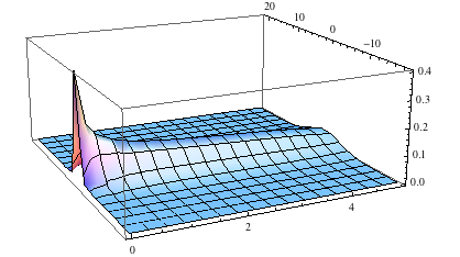
Figure 1: The evolution of distribution $m^{*}_{t},0\leq t\leq 5,-19\leq x\leq 21$.

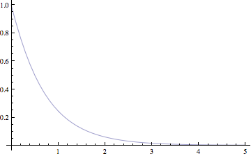
Figure 2: Mean value $\mathbb{E}(m^{*}_{t})$ as a function of time, $0\leq t\leq 5$.

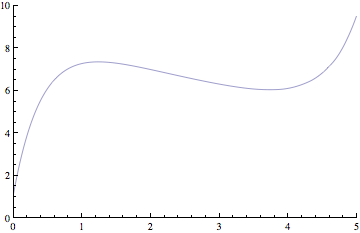
Figure 3: Variance of the distribution $m^{*}_{t}$ as a function of time, $0\leq t\leq 5$.

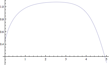
Figure 4: $z(t)$ as a function of time, $0\leq t\leq T$.

We let Player $j$’s state evolution be described by a decoupled stochastic differential equation

$$dx_{j}^{n}(t)=u_{j}(t)dt+\sqrt{\epsilon}\sigma d\mathbb{B}_{j}(t).$$

The risk-sensitive cost functional is given by

$$L(\bar{\gamma}_{j},m^{n};t,\underline{x},\underline{m})=\delta\log\mathbb{E}_{\underline{x},\underline{m}}\left\{\exp\left[\frac{1}{\delta}\left(Q(x^{n}_{j})^{2}\right.\right.\right.\left.\left.\left.+\int_{0}^{T}(q-\mathbb{E}(m^{n}_{t}))(x_{j}^{n})^{2}(t)+\bar{u}_{j}^{2}(t)dt\right)\right]\right\},$$

where $\delta,Q,q$ are positive parameters; hence coupling of the players is only through the cost. The optimal strategy of Player $j$ has the form of

$$\bar{u}_{j}^{*}(t)=-z(t)x,$$ (13)

where $z(t)$ is a solution to the Riccati equation

$$\dot{z}(t)+q-\mathbb{E}(m^{n})-z^{2}(t)(1-\sigma^{2}/\rho^{2})=0,$$

with boundary condition $z(T)=Q$. An explicit solution is given by

$$z(t)=-\frac{\sqrt{q-M}}{\sqrt{L}}\text{tan}\left[\sqrt{L}\sqrt{q-M}(t-T)+\right.\left.\text{arctan}\left(\frac{\sqrt{L}Q}{\sqrt{q-M}}\right)\right],0\leq t\leq T,$$

where $L:=1-\sigma^{2}/\rho^{2}$ and $M:=\mathbb{E}(m^{n})$. The FPK-McV equation reduces to

$$\partial_{t}m_{t}^{*}+\partial_{x}(m_{t}^{*}z(t)x(t))=\frac{\epsilon}{2}\sigma^{2}\partial_{xx}^{2}m^{*}_{t}.$$

We set the parameters as follows: $q=1.2,Q=0.1$, $\delta=100,000$, $\sigma=2.0$, $T=5$ and $\epsilon=5.0$. Let $m^{*}_{0}(x)$ be a normal distribution $\mathcal{N}(1,1)$ and for every $0\leq t\leq T$, $m^{*}_{t}$ vanishes at infinity. In Figure 1, we show the evolution of the distribution $m^{*}_{t}$ and in Figures 2 and 3, we show the mean and the variance of the distribution which affects the optimal strategies in (13). The optimal linear feedback $z(t)$ is illustrated in Figure 4. We can observe that the mean value $\mathbb{E}(m_{t}^{*})$ monotonically decreases from 1.0 and hence the unit cost on state is monotonically increasing. As the state cost increases, the control effort becomes relatively cheaper and therefore we can observe an increment in the magnitude of $z(t)$. However, when the mean value goes beyond 1.08, we observe that the control effort reduces to avoid undershooting in the state.

V-B McKean-Vlasov dynamics

We let the dynamics of an individual player be

$$dx_{j}^{n}(t)=\left(\frac{\beta}{n}\sum_{i=1}^{n}x_{i}^{n}(t)+u_{j}^{n}(t)\right)dt+\sqrt{\epsilon}\sigma d\mathbb{B}_{j}(t),$$ (14)

and take the risk-sensitive cost function to be

$$L=\delta\log E\left\{\exp\left[\frac{1}{\delta}\int_{0}^{T}q(x_{j}^{n}(t))^{2}+(u_{j}^{n}(t))^{2}\right]\right\}.$$

Note that the cost function is independent of other players’ controls or states. As $n\rightarrow\infty$, under regularity conditions,

$$\lim_{n\rightarrow\infty}\sum_{i=1}^{n}\frac{1}{n}x_{i}^{n}(t)=M(t),$$

where $M(t)$ is the mean of the population. The feedback optimal control $\bar{u}_{j}$ in response to the mean field $M(t)$ is characterized by

$$\bar{u}_{j}(t)=-z(t)x_{j}(t)-k(t),$$

where

$$\dot{z}(t)+q-z^{2}(1-\sigma^{2}/\rho^{2}) = 0,\ \ z(T)=0,$$

$$\dot{k}(t)-z(t)k(t)+z(t)M(t) = 0,\ \ k(T)=0,$$

and $\rho^{2}=\frac{\delta}{2\epsilon}$ and $M(t)=\int_{x\in\mathcal{X}}xm(x,t)dx$. The Fokker-Planck-Kolmogorov (FPK) equation is

$$\partial_{t}m(x,t)+\partial_{x}\left(m(x,t)\left(-z(t)x(t)-k(t)\right)+\beta m(x,t)\int_{w}wm(w,t)dw\right)=\frac{\epsilon}{2}\sigma^{2}\partial^{2}_{xx}m(x,t)$$

By solving the ODEs, we find that

$$z(t)=-\sqrt{\bar{q}}\textrm{tan}\left(\sqrt{\hat{q}}(t-T)\right),\ \ 0\leq t\leq T.$$

where $\bar{q}=q/(1-\sigma^{2}/\rho^{2})$ and $\hat{q}=q(1-\sigma^{2}/\rho^{2})$. Let $q=r=1$ and we find the solution

$$k(t)=\textrm{cos}(t-T)\left(\int_{1}^{T}m(\tau)\textrm{sec}(T-\tau)\textrm{tan}(T-\tau)d\tau-\int_{t}^{T}m(\tau^{\prime})\textrm{sec}(T-\tau^{\prime})\textrm{tan}(T-\tau^{\prime})d\tau^{\prime}\right).$$

Let $\sigma=1,\rho=2,\beta=1$ and we show in Figure 5 the evolution of the probability density function $m(x,t)$. The mean $M(t)$ and the variance are shown in Figure 6 and Figure 7, respectively.

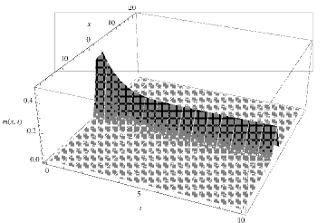
Figure 5: Evolution of the probability density function $m(x,t)$

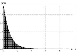
Figure 6: The mean $M(t)$ under equilibrium solution

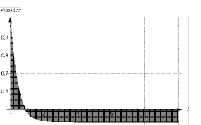
Figure 7: Variance over time under equilibrium solution

VI Concluding remarks

We have studied risk-sensitive mean-field stochastic differential games with state dynamics given by an Itô stochastic differential equation and the cost function being the expected value of an exponentiated integral.

Using a particular structure of state dynamics, we have shown that the mean-field limit of the individual state dynamics leads to a controlled macroscopic McKean-Vlasov equation. We have formulated a risk-sensitive mean-field response framework, and established its compatibility with the density distribution using the controlled Fokker-Planck-Kolmogorov forward equation. The risk-sensitive mean-field equilibria are characterized by coupled backward-forward equations. For the general case, the resulting mean field system is very hard to solve (numerically or analytically) even if the number of equations have been reduced. We have, however, provided generic explicit forms in the particular case of the affine-exponentiated-Gaussian mean-field problem. In addition, we have shown that the risk-sensitive problem can be transformed into a risk-neutral mean-field game problem with the introduction of an additional fictitious player. This allows one to study a novel class of mean field games, robust mean field games, under the Isaacs condition.

An interesting direction that we leave for future research is to extend the model to accommodate multiple classes of players and a drift function which may depend on the other players’ controls. Another direction would be to soften the conditions under which Proposition 5 is valid, such as boundedness and Lipschitz continuity, and extend the result to games with non-smooth coefficients. In this context, one could address a mean field central limit question on the asymptotic behavior of the process $\sqrt{n}\mathbb{E}\left(\parallel x^{n}_{j}(t)-\tilde{x}_{j}(t)\parallel\right).$ Yet another extension would be to the time average risk-sensitive cost functional. Finally, the approach needs to be compared with other risk-sensitive approaches such as the mean-variance criterion and extended to the case where the drift is a function of the state-mean field and the control-mean field.

Proof of Proposition 5.

Under the stated standard assumptions on the drift $f$ and variance $\sigma$, the forward stochastic differential equation has a unique solution adapted to the filtration generated by the Brownian motions. We want to show that

$$\mathbb{E}\left(\sup_{t\in[0,T]}\parallel x^{n}_{j}(t)-\tilde{x}_{j}(t)\parallel\right)\leq\frac{C_{T}}{\sqrt{n}},$$

where $C_{T}$ is a positive number which only depends on the bounds, $T$ and the Lipschitz constants of the coefficients of the drifts and the variance term. First we observe that for a fixed control $u,$ the averaging terms $\frac{1}{n}\sum_{i=1}^{n}f(t,x_{j},u,x_{i})$ and $\frac{1}{n}\sum_{i=1}^{n}\sigma(t,x_{j},u,x_{i})$ are measurable, bounded and Lipschitz with the respect to the state and uniformly with the respect to time.

Second, we observe that the bound on the Lipschitz constants of the coefficients do not depend on the population size $n.$

Hence, $\int f(t,x,u,x^{\prime})\ m_{t}(dx^{\prime})$ and $\int\sigma(t,x,u,x^{\prime})\ m_{t}(dx^{\prime})$ are bounded and Lipschitz uniformly with the respect to $t.$ Moreover, these coefficients are deterministic. This means that there is a unique solution to the limiting SDE and that solution is measurable with the filtration generated by the mutually independent Brownian motions.

Third, we evaluate the gap between the coefficients in order to obtain an estimate of the two processes. We start by evaluating the gap

$$\mathbb{E}\left(\left\|\frac{1}{n}\sum_{i=1}^{n}f(t,x,u,x_{i})-\int f(t,x,u,x^{\prime})\ m_{t}(dx^{\prime})\right\|^{2}\right)$$

Notice that $f$ returns a $k-$dimensional vector and $x$ belongs to $\mathbb{R}^{k}$. By reordering the above expression (in $2-$norm), we obtain

$$\sum_{l=1}^{k}\mbox{var}\left(\frac{1}{n}\sum_{i=1}^{n}f_{l}(t,x_{j},u,x_{i})\right)\leq\frac{k}{n}(1+\max_{l}b_{l})^{2}\leq\frac{C_{T}}{n},$$

where $\mbox{var}(X)$ denotes the variance of $X$ and $b_{l}$ is a bound on the $l-$th component of the drift term. (This exists because we have assumed boundedness conditions on the coefficients).

Following a similar reasoning, we obtain the bounds on the second term in $\sigma$, i.e.,

$$\sum_{l,l^{\prime}}\mbox{var}\left(\frac{1}{n}\sum_{i=1}^{n}\sigma_{ll^{\prime}}(t,x_{j},u,x_{i})\right)\leq\frac{k}{n}(1+\max_{ll^{\prime}}c_{ll^{\prime}})^{2}\leq\frac{C_{T}}{n},$$

where $c_{ll^{\prime}}$ is a bound on the entries $(l,l^{\prime})-$ of the matrix $\sigma$.

Now we use the Lispchitz conditions and standard Gronwall estimates to deduce that the mean of the quadratic gap between the two stochastic processes (starting from $x$ at time $0$) is in order of $\frac{1}{n}.$

∎

Proof of Theorem 1.

Under the stated regularity and boundedness assumptions, there is a solution to the McKean-Vlasov FPK equation. Suppose that (i) and (ii) are satisfied. Then, $m_{t}=m^{*}(t,u^{*}(t))$ is the solution of the mean-field limit state dynamics, i.e., the macroscopic McKean-Vlasov PDE when $m$ is substituted into the HJB equation. By fixing $f^{*},c^{*},\sigma,$ we obtain a novel HJB equation for the mean-field stochastic game. Since the new PDE admits a solution according to (ii), the control $u^{*}(t)=u(t,x)$ minimizing $\partial_{x}v\cdot f+c,$ is a best response to $m^{*}$ at time $t.$ The optimal response of the individual player generates a mean-field limit which in law is a solution of the FPK PDE and the players compute their controls as a function of this mean-field. Thus, the consistency between the control, the state and the mean field is guaranteed by assumption (i). It follows that $(u^{*},m^{*})$ is a solution to the fixed-point problem i.e., a mean-field equilibrium, and a strongly time-consistent one.

Now, we look at the quadratic instantaneous cost case. In that case, we obtain the risk-sensitive equations provided in Proposition 3. The fact that any convergent subsequence of best-response to $m^{n}$ is a best response to $m^{*}$ and the fact that $u^{*}$ is an $\epsilon^{*}-$best response to the mean-field limit $m^{*}$ follow from mean-field convergence of order $O\left(\frac{1}{\sqrt{n}}\right)$ and the continuity of the risk-sensitive quadratic cost functional. ∎

Proof of Theorem 3.

We provide a sufficient condition for the risk-sensitive mean field game to have at most one smooth solution. Suppose $\delta>0,$ and $\sigma$ is positive constant. Let $H$ be the Hamiltonian associated with the risk-neutral mean field system. Then the Hamiltonian for the risk-sensitive mean field system is $\tilde{H}(x,p,m)=H+(\frac{\epsilon\sigma^{2}}{2\delta})\parallel p\parallel^{2}.$ Assume that the dependence on $m$ is local, i.e., it is function of $m(x).$

The generic expression for the optimal control is given by $u^{*}=\partial_{p}{H}(x,\partial_{x}v,m_{t}(x))$ (note that the generic feedback control is expressed in terms of $H$, and not of $\tilde{H}$).

Suppose that there exist two smooth solutions $(\hat{v}_{1},\hat{m}_{1}),$ $(\hat{v}_{2},\hat{m}_{2})$ to the (normalized) risk-sensitive mean field system. Now, consider the function $t\longmapsto\int_{x\in\mathcal{X}}(\hat{v}_{2}(x)-\hat{v}_{1}(x))(\hat{m}_{2}(x)-\hat{m}_{1}(x))dx.$ Observe that this function is $0$ at time $t=0$ because the measures coincide initially, and the function is equal to $0$ at time $t=T$ because the final values coincide. Therefore, the function will be identically $0$ in $[0,T]$ if we show that it is monotone. This will imply that the integrand is zero, and hence one of the two terms $(\hat{v}_{2}(x)-\hat{v}_{1}(x))$ or $(\hat{m}_{2,t}(x)-\hat{m}_{1,t}(x))$ should be $0.$ Then, if the measures are identical, we use the HJB equation to obtain the result. If the value functions are identical, we can use the FPK equation to show the uniqueness of the measure. Thus, it remains to find a sufficient condition for monotonicity, that is, a sufficient condition under which the quantity $\int_{x\in\mathcal{X}}(\hat{v}_{2}(x)-\hat{v}_{1}(x))(\hat{m}_{2}(x)-\hat{m}_{1}(x))dx$ is monotone in time. We compute the following time derivative:

$$S(t):=\frac{d}{dt}\left[\int_{x\in\mathcal{X}}(\hat{v}_{2}(x)-\hat{v}_{1}(x))(\hat{m}_{2}(x)-\hat{m}_{1}(x))dx\right].$$

We interchange the order of the integral and the differentiation and use time derivative of a product to arrive at;

$$S(t) = \int_{x\in\mathcal{X}}(\partial_{t}\hat{v}_{2}-\partial_{t}\hat{v}_{1})(\hat{m}_{2}(x)-\hat{m}_{1}(x))dx+$$

$$\int_{x\in\mathcal{X}}(\hat{v}_{2}-\hat{v}_{1})(\partial_{t}\hat{m}_{2}(x)-\partial_{t}\hat{m}_{1}(x))dx$$

Now we expand the first term $A:=\int_{x\in\mathcal{X}}(\partial_{t}\hat{v}_{2}-\partial_{t}\hat{v}_{1})(\hat{m}_{2}(x)-\hat{m}_{1}(x))dx.$ Consider the two HJB equations:

$$\partial_{t}\hat{v}_{1}+\tilde{H}(x,\partial_{x}\hat{v}_{1},\hat{m}_{1}(x))+\frac{1}{2}\sigma^{2}\partial^{2}_{xx}\hat{v}_{1}=0,$$

$$\partial_{t}\hat{v}_{2}+\tilde{H}(x,\partial_{x}\hat{v}_{2},\hat{m}_{2}(x))+\frac{1}{2}\sigma^{2}\partial^{2}_{xx}\hat{v}_{2}=0$$

To compute $A$, we take the difference between the two HJB equations above and multiply by $\hat{m}_{2}-\hat{m}_{1},$ which gives

$$\partial_{t}\hat{v}_{2}-\partial_{t}\hat{v}_{1}=-\tilde{H}(x,\partial_{x}\hat{v}_{2},\hat{m}_{2})+\tilde{H}(x,\partial_{x}\hat{v}_{1},\hat{m}_{1})-\frac{1}{2}\sigma^{2}\partial^{2}_{xx}\hat{v}_{2}+\frac{1}{2}\sigma^{2}\partial^{2}_{xx}\hat{v}_{1}$$

Hence,

$${A} := \int_{x}[\partial_{t}\hat{v}_{2}-\partial_{t}\hat{v}_{1}](\hat{m}_{2}(x)-\hat{m}_{1}(x))dx$$

$$= -\int_{x}\tilde{H}(x,\partial_{x}\hat{v}_{2},\hat{m}_{2})(\hat{m}_{2}(x)-\hat{m}_{1}(x))dx$$

$$+\int_{x}\tilde{H}(x,\partial_{x}\hat{v}_{1},\hat{m}_{1})(\hat{m}_{2}(x)-\hat{m}_{1}(x))dx$$

$$-\int_{x}\frac{1}{2}\sigma^{2}\partial^{2}_{xx}(\hat{v}_{2})(\hat{m}_{2}(x)-\hat{m}_{1}(x))dx$$

$$+\int_{x}\sigma^{2}\frac{1}{2}\partial^{2}_{xx}(\hat{v}_{1})(\hat{m}_{2}(x)-\hat{m}_{1}(x))dx$$

Next we expand the second term $B:=\int_{x\in\mathcal{X}}(\partial_{t}\hat{m}_{2}-\partial_{t}\hat{m}_{1})(\hat{v}_{2}-\hat{v}_{1})dx.$ Note that the Laplacian terms are canceled by integration by parts in the expression $A+B$. By collecting all the terms in $A+B$, we obtain

$$A+B = -\int_{x}\tilde{H}(x,\partial_{x}\hat{v}_{2},\hat{m}_{2})(\hat{m}_{2}(x)-\hat{m}_{1}(x))dx$$

$$+\int_{x}\tilde{H}(x,\partial_{x}\hat{v}_{1},\hat{m}_{1})(\hat{m}_{2}(x)-\hat{m}_{1}(x))dx$$

$$+\int_{x}\hat{m}_{2}(x)[\partial_{p}{H}(x,\partial_{x}\hat{v}_{2},\hat{m}_{2})](\partial_{x}\hat{v}_{2}-\partial_{x}\hat{v}_{1})dx$$

$$-\int_{x}\hat{m}_{1}(x)[\partial_{p}{H}(x,\partial_{x}\hat{v}_{1},\hat{m}_{1})](\partial_{x}\hat{v}_{2}-\partial_{x}\hat{v}_{1})dx$$

Letting $S(t)=A+B$, we introduce

$$\hat{m}_{\lambda}:=(1-\lambda)\hat{m}_{1}+\lambda\hat{m}_{2}=\hat{m}_{1}+\lambda(\hat{m}_{2}-\hat{m}_{1}).$$

The measure $\hat{m}_{\lambda}$ starts with $\hat{m}_{1}$ for the parameter $\lambda=0$ and yields the measure $\hat{m}_{2}$ for $\lambda=1.$ Similarly define

$$\hat{v}_{\lambda}:=(1-\lambda)\hat{v}_{1}+\lambda\hat{v}_{2}.$$

Introduce an auxiliary integral parameterized by $\lambda.$

$$C_{\lambda} := -\int_{x}\tilde{H}(x,\partial_{x}\hat{v}_{\lambda},\hat{m}_{\lambda})(\hat{m}_{\lambda}(x)-\hat{m}_{1}(x))dx$$

$$+\int_{x}\tilde{H}(x,\partial_{x}\hat{v}_{1},\hat{m}_{1})(\hat{m}_{\lambda}(x)-\hat{m}_{1}(x))dx$$

$$+\int_{x}\hat{m}_{\lambda}(x)[\partial_{p}{H}(x,\partial_{x}\hat{v}_{\lambda},\hat{m}_{\lambda})](\partial_{x}\hat{v}_{\lambda}-\partial_{x}\hat{v}_{1})dx$$

$$-\int_{x}\hat{m}_{1}(x)[\partial_{p}{H}(x,\partial_{x}\hat{v}_{1},\hat{m}_{1})](\partial_{x}\hat{v}_{\lambda}-\partial_{x}\hat{v}_{1})dx$$

Substituting the terms $\hat{v}_{\lambda}-\hat{v}_{1}=\lambda(\hat{v}_{2}-\hat{v}_{1})$ and $\hat{m}_{\lambda}-\hat{m}_{1}=\lambda(\hat{m}_{2}-\hat{m}_{1}),$ we obtain

$$\frac{C_{\lambda}}{\lambda} := -\int_{x}\tilde{H}(x,\partial_{x}\hat{v}_{\lambda},\hat{m}_{\lambda})(\hat{m}_{2}(x)-\hat{m}_{1}(x))dx$$

$$+\int_{x}\tilde{H}(x,\partial_{x}\hat{v}_{1},\hat{m}_{1})(\hat{m}_{2}(x)-\hat{m}_{1}(x))dx$$

$$+\int_{x}\hat{m}_{\lambda}(x)[\partial_{p}{H}(x,\partial_{x}\hat{v}_{\lambda},\hat{m}_{\lambda})](\partial_{x}\hat{v}_{2}-\partial_{x}\hat{v}_{1})dx$$

$$-\int_{x}\hat{m}_{1}(x)[\partial_{p}{H}(x,\partial_{x}\hat{v}_{1},\hat{m}_{1})](\partial_{x}\hat{v}_{2}-\partial_{x}\hat{v}_{1})dx$$

Using the continuity of the terms (of the RHS) above and the compactness of $\mathcal{X},$ we deduce that

$$\lim_{\lambda\longrightarrow 0}\frac{C_{\lambda}}{\lambda}=0.$$

We next find a condition under which the one-dimensional function $\lambda\longmapsto\frac{C_{\lambda}}{\lambda}$ is monotone in $\lambda.$ We need to compute the variations of

$$\frac{d}{d\lambda}\left(\frac{C_{\lambda}}{\lambda}\right).$$

Suppose that $(x,p,m)\longmapsto\tilde{H}(x,p,m)$ is twice continuously differentiable with the respect to $(p,m).$ Then,

$$\frac{d}{d\lambda}\left(\frac{C_{\lambda}}{\lambda}\right) = -\int_{x}\left[\partial_{p}\tilde{H}(x,\partial_{x}\hat{v}_{\lambda},\hat{m}_{\lambda})(\partial_{x}\hat{v}_{2}-\partial_{x}\hat{v}_{1})\right](\hat{m}_{2}(x)-\hat{m}_{1}(x))dx$$

$$-\int_{x}\left[\partial_{m}\tilde{H}(x,\partial_{x}\hat{v}_{\lambda},\hat{m}_{\lambda})(\hat{m}_{2}(x)-\hat{m}_{1}(x))\right](\hat{m}_{2}(x)-\hat{m}_{1}(x))dx$$

$$+\int_{x}\partial_{\lambda}\left(\hat{m}_{\lambda}(x)[\partial_{p}{H}(x,\partial_{x}\hat{v}_{\lambda},\hat{m}_{\lambda})]\right)(\partial_{x}\hat{v}_{2}-\partial_{x}\hat{v}_{1})dx$$

$$\frac{d}{d\lambda}\left(\frac{C_{\lambda}}{\lambda}\right) = -\int_{x}\partial_{p}\tilde{H}(x,\partial_{x}\hat{v}_{\lambda},\hat{m}_{\lambda})(\partial_{x}\hat{v}_{2}-\partial_{x}\hat{v}_{1})(\hat{m}_{2}(x)-\hat{m}_{1}(x))dx$$

$$-\int_{x}\partial_{m}\tilde{H}(x,\partial_{x}\hat{v}_{\lambda},\hat{m}_{\lambda})(\hat{m}_{2}(x)-\hat{m}_{1}(x))^{2}dx$$

$$+\int_{x}(\hat{m}_{2}-\hat{m}_{1})[\partial_{p}{H}(x,\partial_{x}\hat{v}_{\lambda},\hat{m}_{\lambda})](\partial_{x}\hat{v}_{2}-\partial_{x}\hat{v}_{1})dx$$

$$+\int_{x}\hat{m}_{\lambda}\partial_{\lambda}[\partial_{p}{H}(x,\partial_{x}\hat{v}_{\lambda},\hat{m}_{\lambda})](\partial_{x}\hat{v}_{2}-\partial_{x}\hat{v}_{1})dx$$

Computation of the term $\hat{m}_{\lambda}(x)\partial_{\lambda}\left([\partial_{p}{H}(x,\partial_{x}\hat{v}_{\lambda},\hat{m}_{\lambda})]\right)$ yields

$$D_{\lambda} = \partial_{\lambda}[\partial_{p}{H}(x,\partial_{x}\hat{v}_{\lambda},\hat{m}_{\lambda})]$$

$$= \partial^{2}_{pp}{H}.(\partial_{x}\hat{v}_{2}-\partial_{x}\hat{v}_{1})+\partial^{2}_{mp}{H}.(\hat{m}_{2}-\hat{m}_{1})$$

and we obtain

$$\frac{d}{d\lambda}\left(\frac{C_{\lambda}}{\lambda}\right) = -\int_{x}\partial_{p}\tilde{H}(x,\partial_{x}\hat{v}_{\lambda},\hat{m}_{\lambda})(\partial_{x}\hat{v}_{2}-\partial_{x}\hat{v}_{1})(\hat{m}_{2}(x)-\hat{m}_{1}(x))dx$$

$$-\int_{x}\partial_{m}\tilde{H}(x,\partial_{x}\hat{v}_{\lambda},\hat{m}_{\lambda})(\hat{m}_{2}(x)-\hat{m}_{1}(x))^{2}dx$$

$$+\int_{x}(\hat{m}_{2}-\hat{m}_{1})[\partial_{p}{H}(x,\partial_{x}\hat{v}_{\lambda},\hat{m}_{\lambda})](\partial_{x}\hat{v}_{2}-\partial_{x}\hat{v}_{1})dx$$

$$+\int_{x}\hat{m}_{\lambda}\partial^{2}_{pp}{H}.(\partial_{x}\hat{v}_{2}-\partial_{x}\hat{v}_{1})^{2}+\hat{m}_{\lambda}\partial^{2}_{mp}{H}.(\hat{m}_{2}-\hat{m}_{1})(\partial_{x}\hat{v}_{2}-\partial_{x}\hat{v}_{1})$$

The first and the third lines differ by

$$-\int_{x}\left(\frac{\epsilon\sigma^{2}}{\delta}\langle.,\nabla_{x}\hat{v}\rangle\right)\left(\partial_{x}\hat{v}_{2}-\partial_{x}\hat{v}_{1}\right)\left(\hat{m}_{2}(x)-\hat{m}_{1}(x)\right)dx.$$

Hence, we obtain

$$\frac{d}{d\lambda}\left(\frac{C_{\lambda}}{\lambda}\right) = \int_{x}m_{\lambda}(\partial_{x}\hat{v}_{2}-\partial_{x}\hat{v}_{1},\hat{m}_{2}-\hat{m}_{1})\left(\begin{array}[]{cc}a_{11}&a_{12}\\ a_{21}&a_{22}\end{array}\right)\left(\begin{array}[]{c}\partial_{x}\hat{v}_{2}-\partial_{x}\hat{v}_{1}\\ \hat{m}_{2}-\hat{m}_{1}\end{array}\right)dx,$$ (19)

where

$$a_{11}:=\partial_{pp}^{2}{H},$$

$$a_{21}:=\frac{1}{2}\partial_{mp}^{2}\tilde{H}=\frac{1}{2}\partial_{mp}^{2}H-\frac{\epsilon\sigma^{2}}{2\delta}p/m,$$

$$a_{21}:=\frac{1}{2}(\partial_{pm}^{2}\tilde{H})^{\prime}-\frac{\epsilon\sigma^{2}}{2\delta}\frac{p}{m}=\frac{1}{2}(\partial_{pm}^{2}H)^{\prime}-\frac{\epsilon\sigma^{2}}{2\delta}\frac{p}{m},$$

$$a_{22}:=-\frac{\partial_{m}\tilde{H}}{m}.$$

Suppose that for all $(x,p,m)\in\mathcal{X}\times\mathbb{R}^{d}\times\mathbb{R}_{+},$ the matrix

$$\left(\begin{array}[]{cc}a_{11}&a_{12}\\ a_{21}&a_{22}\end{array}\right)\succ 0.$$

Then, the monotonicity follows, and this completes the proof. ∎

References

- [1] S. Adlakha, R. Johari, G. Weintraub, and A. Goldsmith. Oblivious equilibrium for large-scale stochastic games with unbounded costs. Proc. IEEE CDC, Cancun, Mexico, pages 5531–5538, 2008.
- [2] T. Başar. Nash equilibria of risk-sensitive nonlinear stochastic differential games. J. of Optimization Theory and Applications, 100(3):479–498, 1999.
- [3] M. Bardi. Explicit solutions of some linear-quadratic mean field games. Workshop on Mean Field Games, Roma, 2011.
- [4] T. Başar and G. J. Olsder. Dynamic noncooperative game theory, volume 23. Society for Industrial and Applied Mathematics (SIAM), 1999.
- [5] A. Bensoussan, K. C. J. Sung, S. C. P. Yam, and S. P. Yung. Linear-quadratic mean field games. avaliable at http://www.sta.cuhk.edu.hk/scpy/Preprints/, 2011.
- [6] A. Bensoussan and J.H. van Schuppen. Optimal control of partially observable stochastic systems with an exponential-of-integral performance index. SIAM J. Control and Optimization, 23:599–613, 1985.
- [7] J. Bergin and D. Bernhardt. Anonymous sequential games with aggregate uncertainty. J. Mathematical Economics, 21:543–562, 1992.
- [8] F. Cucker and S. Smale. Emergent behavior in flocks. IEEE Trans. Automat. Control, 52, 2007.
- [9] F. Cucker and S. Smale. On the mathematics of emergence. Japan. J. Math., 2:197–227, 2007.
- [10] D. A. Dawson. Critical dynamics and fluctuations for a mean-field model of cooperative behavior. Journal of Statistical Physics, 31:29–85, 1983.
- [11] C. Graham. Chaoticity on path space for a queueing network with selection of the shortest queue among several. Journal of Applied Probability, 37:198–211, 2000.
- [12] O. Guéant. Mean field games - uniqueness result. Course notes, 2011.
- [13] O Guéant, Jean-Michel Lasry, and Pierre-Louis Lions. Mean field games and applications. Springer: Paris-Princeton Lectures on Mathematical Finance, Eds. René Carmona, Nizar Touzi, 2010.
- [14] Tembine H. and M. Huang. Mean field stochastic difference games: McKean-Vlasov dynamics. CDC-ECC, 50th IEEE Conference on Decision and Control and European Control Conference, Orlando, Florida, December 12-15 2011.
- [15] M. Huang, P. E. Caines, and Malhamé R. P. Large-population cost-coupled LQG problems with nonuniform agents: Individual-mass behavior and decentralized -Nash equilibria. IEEE Trans. Automat. Control, 52:1560–1571, 2007.
- [16] M. Huang, R. P. Malhamé, and P. E. Caines. Large population stochastic dynamic games: closed-loop McKean-Vlasov systems and the Nash certainty equivalence principle. Commun. Inf. Syst., 6(3):221–252, 2006.
- [17] M. Y. Huang, P. E. Caines, and R. P. Malhamé. Individual and mass behaviour in large population stochastic wireless power control problems : Centralized and Nash equilibrium solution. IEEE Conference on Decision and Control, HA, USA, pages 98 – 103, December 2003.
- [18] D.H. Jacobson. Optimal stochastic linear systems with exponential performance criteria and their relation to deterministic differential games. IEEE Trans. Automat. Contr., 18(2):124–131, 1973.
- [19] B. Jovanovic and R. W. Rosenthal. Anonymous sequential games. Journal of Mathematical Economics, 17:77–87, 1988.
- [20] M. Kac. Foundations of kinetic theory. Proc. Third Berkeley Symp. on Math. Statist. and Prob., 3:171–197, 1956.
- [21] P. Kotolenez and T. Kurtz. Macroscopic limits for stochastic partial differential equations of McKean-Vlasov type. Probability theory and related fields, 146(1):189–222, 2010.
- [22] Y. Kuramoto. Chemical oscillations, waves, and turbulence. Springer, 1984.
- [23] J.M. Lasry and P.L. Lions. Mean field games. Japan. J. Math., 2:229–260, 2007.
- [24] P. L. Lions. Cours jeux à champ moyens et applications. College de France, 2010.
- [25] R.P. Malhame M.Y. Huang and P.E. Caines. Large population stochastic dynamic games: Closed loop McKean-Vlasov systems and the Nash certainty equivalence principle. Special issue in honour of the 65th birthday of Tyrone Duncan, Communications in Information and Systems, 6(3):221–252, 2006.
- [26] B. Oksendal. Stochastic Differential Equations: An Introduction with Applications (Universitext). Springer, 6th edition, 7 2003.
- [27] Z. Pan and T. Başar. Model simplification and optimal control of stochastic singularly perturbed systems under exponentiated quadratic cost. SIAM J. Control and Optimization, 34(5):1734–1766, September 1996.
- [28] A. S. Sznitman. Topics in propagation of chaos. In P.L. Hennequin, editor, Springer Verlag Lecture Notes in Mathematics 1464, Ecole d’Eté de Probabilités de Saint-Flour XI (1989), pages 165–251, 1991.
- [29] Y. Tanabe. The propagation of chaos for interacting individuals in a large population. Mathematical Social Sciences, 51:125–152, 2006.
- [30] H. Tembine. Mean field stochastic games. Notes, Supelec, October 2010.
- [31] H Tembine. Mean field stochastic games: Convergence, Q/H-learning and optimality. In Proc. American Control Conference (ACC), San Francisco, California, USA, 2011.
- [32] H Tembine, S. Lasaulce, and M. Jungers. Joint power control-allocation for green cognitive wireless networks using mean field theory. Proc. 5th IEEE Intl. Conf. on Cogntitive Radio Oriented Wireless Networks and Communications (CROWNCOM), pages 1–5, 2010.
- [33] H. Tembine, J. Y. Le Boudec, R. ElAzouzi, and E. Altman. Mean field asymptotic of Markov decision evolutionary games and teams. Proc. International Conference on Game Theory for Networks (GameNets), Istanbul, Turkey, May 13-15, 2009., pages 140–150, May 2009.
- [34] G. Y. Weintraub, L. Benkard, and B. Van Roy. Oblivious equilibrium: A mean field approximation for large-scale dynamic games. Advances in Neural Information Processing Systems, 18, 2005.
- [35] P Whittle. Risk-sensitive linear quadratic Gaussian control. Advances in Applied Probability, 13:764–777, 1981.
- [36] H. Yin, P. G. Mehta, S. P. Meyn, and U. V. Shanbhag. Synchronization of coupled oscillators is a game. Proc. American Control Conference (ACC), Baltimore, MD, pages 1783–1790, 2010.
- [37] J. Yong and X. Y. Zhou. Stochastic Controls. Springer, 1999.