Spin convertance at magnetic interfaces

Abstract

Exchange interaction between conduction electrons and magnetic moments at magnetic interfaces leads to mutual conversion between spin current and magnon current. We introduce a concept of spin convertance which quantitatively measures magnon current induced by spin accumulation and spin current created by magnon accumulation at a magnetic interface. We predict several phenomena on charge and spin drag across a magnetic insulator spacer for a few layered structures.

I Introduction

In spintronics, spin current, which is conventionally defined as the difference of electric currents of spin-up and spin-down conduction electrons, plays a pivotal role in propagating spin information from one place to another. Many spin dependent properties, such as giant magnetoresistance Fert ; Grunberg , spin transfer torques Slonczewski ; Berger and spin Hall effect Hirsch ; Zhang00 , are directly related to spin current. Spin current has several unique properties compared to charge current: 1) it is considered as a flow of angular momentum while the conventional current is a flow of charge, 2) the total spin current is not a conserved quantity even in the steady state condition; it can be transferred and/or lost due to spin-dependent scattering, and 3) spin current has both transverse and longitudinal components whose decaying length scales are quite different in a ferromagnetic medium. Recently, the concept of spin current has been extended to spin wave current since spin waves carry angular momenta as well Kajiwara10 . There are two types of spin wave currents. One is magnetostatic wave propagation Kajiwara10 ; Xiao12 ; Wu11 ; Nowak11 ; Wang11 for which the classical magnetization is temporal and spatially dependent. An example is a moving domain wall driven by a magnetic field or by an electric current. Although such magnetostatic spin waves may carry angular momentum, they are not quasi-particles in that there are no particle numbers associated with these waves. The other spin wave current is a true quasi-particle current known as magnon current. A magnon is a quantum object (particle) that represents low excitation state of ferromagnets. In equilibrium, the number of magnons $N_{\mathbf{q}}$ can be cast into a simple Boson distribution $N_{\mathbf{q}}^{0}=[e^{E_{\mathbf{q}}/k_{B}T}-1]^{-1}$ where $E_{\mathbf{q}}$ is the magnon energy. Similar to the electron spin, each magnon carries an angular momentum $-\hbar$. In thermal equilibrium, there is no magnon current since there are an equal number of magnons moving in all directions.

In our earlier paper Zhang12 , we showed that the non-equilibrium magnon accumulation and magnon current can be treated semiclassically, similar to the spin transport properties of conduction electrons. We found that the non-equilibrium electron spin current in metal can convert into a magnon current of a magnetic insulator through the interfacial exchange interaction. The magnon current then subsequently diffuses inside the magnetic insulator. The magnon diffusion process may be described by the diffusion equation. Among other things, we predicted that an electric current applied in one metallic layer can induce an electric current in another metallic layer separated by a magnetic insulator via magnon mediated angular momentum transfer. In this paper, we extend our theory to include a general boundary condition for the spin convertibility at metal$\mid$magnetic-insulator interfaces and then, we calculate the electric drag in a few realizations. The paper is organized as follows. In Sec. II, we summarize the general boundary conditions at the interfaces between metals and magnetic insulators. In particular, we introduce a quantity, named as spin convertance, which quantitatively characterizes conversion effectiveness among spin/magnon accumulation and magnon/spin current at a magnetic interface. In Sec. III, we calculate the spin convertance by using the microscopic s-d exchange interaction. In Sec. IV, we present the general solutions for several layered structures with a magnetic insulator layer (MIL) and discuss some limiting cases. Finally, we summarize our results.

II Summary of boundary conditions

We consider a simple bilayer consisting of a metallic layer in contact with a MIL. The angular momentum in a metal is carried by conduction electrons while in a MIL, it is carried by magnons. In the semiclassical approximation, spin transport properties can be described by the Boltzmann distributions of electrons and magnons Zhang12 . The boundary conditions are to link the non-equilibrium electron distribution function of the metal to the magnon distribution function of the MIL. Within the model of the s-d exchange interaction (see Sec. III), the total angular momentum is conserved and thus for an ideal interface the first boundary condition would be

$$j_{t}(0^{-})=j_{t}(0^{+})$$ (1)

where $j_{t}$ is the total angular momentum current, and we assign the interface at $x=0$. If we consider the left layer as a non-magnetic metal ($x<0$), the angular momentum is carried by conduction electrons only and thus $j_{t}(0^{-})=j_{s}(0^{-})$ where $j_{s}$ denotes the conventional spin current density. For the MIL on the right, the angular momentum is carried by magnons only and thus $j_{t}(0^{+})=j_{m}(0^{+})$ where $j_{m}$ corresponds to the magnon current density. Therefore, we may rewrite Eq. (1) as

$$j_{s}(0^{-})=j_{m}(0^{+})$$ (2)

Note that for a magnetic metal, both spin and magnon current contribute to the total angular momentum current.

The second boundary condition is the relation among the electron spin accumulation $\delta m_{s}(0^{-})$, the magnon accumulation $\delta m_{m}(0^{+})$, and the total angular momentum current $j_{t}(0)$,

$$G_{em}\delta m_{s}(0^{-})-G_{me}\delta m_{m}(0^{+})=j_{t}(0)$$ (3)

where the two coefficients $G_{em}$ and $G_{me}$ will be calculated within the s-d model in the next section. The physics of this boundary condition is rather transparent: the first term represents the generation of the magnon current in the presence of electron spin accumulation and the second term describes the spin current produced by magnon accumulation. The combination of these two processes at the interface yields the total interface spin current. We immediately note that Eq. (3) is analogous to the case of spin current between two metallic layers in which the boundary condition is $G_{\sigma}\mu_{\sigma}(0^{+})-G_{\sigma}\mu_{\sigma}(0^{-})=j_{\sigma}(0)$ where $\mu_{\sigma}$ denotes the spin dependent chemical potential ($\sigma=\pm 1$ or $\uparrow(\downarrow)$ corresponds to spin-up (down)) which is proportional to spin accumulation, and $G_{\sigma}$ characterizes the interfacial spin conductance Valet93 . With this analogy, we may identify the coefficients $G_{em}$ ($G_{me}$) as the interface conductance for the conversion of the spin (magnon) accumulation to the magnon (spin) current; we simply call $G_{em}$ and $G_{me}$ spin convertance for convenience hereafter.

We point out that the boundary condition, Eq. (3), is different from what we proposed in the earlier paper Zhang12 where we related the spin and magnon accumulation via a local magnetic susceptibility. Clearly, such approximation corresponds to an ideal case in which the interface spin resistance is zero or the spin convertance is infinite. In the next section, we shall calculate these spin convertances and show that they are in fact finite and thus the magnon mediated electric drag effect predicted in Ref. Zhang12 was overestimated by one order of magnitude.

III Microscopic calculation of spin convertance

We start with the s-d exchange coupling at a metal$\mid$MIL interface,

$$\hat{H}_{sd}=-J_{sd}\sqrt{\frac{S}{2N_{s}}}\underset{\mathbf{k},\mathbf{q},\mathbf{k}\prime}{\sum}(a_{\mathbf{q}}^{{\dagger}}c_{\mathbf{k}\uparrow}^{{\dagger}}c_{\mathbf{k}\prime\downarrow}+a_{\mathbf{q}}c_{\mathbf{k}\prime\downarrow}^{{\dagger}}c_{\mathbf{k}\uparrow})\delta_{\mathbf{k}\prime=\mathbf{q+k}}$$ (4)

where $c_{\mathbf{k}\uparrow}^{{\dagger}}$ ($c_{\mathbf{k}\uparrow}$) and $c_{\mathbf{k}\downarrow}^{{\dagger}}$ ($c_{\mathbf{k}\downarrow}$) are the creation (annihilation) operators for spin-up and spin spin-down electrons respectively, $a_{\mathbf{q}}^{{\dagger}}$ ($a_{\mathbf{q}}$) is the creation (annihilation) operator for magnons, $S$ is the spin per atom of the MIL, and $N_{s}$ is the number of atomic spins of the MIL at the interface. The exchange coupling strength $J_{sd}$ is given by the exchange integral with the overlapped wavefunctions of the conduction electrons and the magnetic ions. Since we do not know the detailed orbitals for the interface states, the magnitude of $J_{sd}$ at interface is less known compared to that in bulk materials and we will treat it as a parameter.

The above exchange interaction gives rise to angular momentum transfer between the electron spins at the metallic side and the magnons at the MIL side. In equilibrium, the net spin current across the interface is zero. At non-equilibrium when there is a spin accumulation at $x=0^{-}$ or a magnon accumulation at $x=0^{+}$, a net magnon/spin current may be present across the interface. In Fig. 1, we illustrate two angular momentum transfer processes. The total angular momentum current across the interface should be caused by both processes. We shall calculate them separately below.

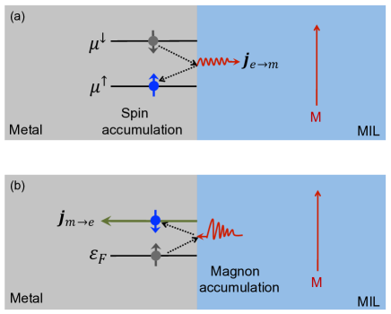
Figure 1: Spin angular momentum transfer at a metal$\mid$MIL interface. The upper (lower) panel describes magnon current $j_{e\rightarrow m}$ (spin current $j_{m\rightarrow e}$) generated by spin accumulation $\delta m_{s}$ (magnon accumulation $\delta m_{m}$) at the interface.

Magnon current generated by spin accumulation at the interface is defined as

$$j_{e\rightarrow m}\equiv\left\langle\frac{\mu_{B}}{i\hbar A_{I}}\left[\sum_{\mathbf{k}}(c_{\mathbf{k}\uparrow}^{{\dagger}}c_{\mathbf{k}\uparrow}-c_{\mathbf{k}\downarrow}^{{\dagger}}c_{\mathbf{k}\downarrow}),\hat{H}_{sd}\right]\right\rangle$$ (5)

where $<>$ refers to the thermal averaging over all states and $A_{I}$ is the area of the interface. By explicitly working out the above commutator and by using the Fermi-golden rule, we have

$$j_{e\rightarrow m}=\frac{2\pi\mu_{B}S}{A_{I}\hbar}\left(\frac{J_{sd}}{N_{s}}\right)^{2}\underset{\mathbf{k},\mathbf{q},\mathbf{k}\prime}{\sum}\left[(N_{\mathbf{q}}+1)(1-f_{\mathbf{k}\uparrow})f_{\mathbf{k}\prime\downarrow}-N_{\mathbf{q}}(1-f_{\mathbf{k}\prime\downarrow})f_{\mathbf{k}\uparrow}\right]\delta(\varepsilon_{\mathbf{k}}+E_{q}-\varepsilon_{\mathbf{k}\prime})$$ (6)

where $N_{\mathbf{q}}$ and $f_{\mathbf{k}\sigma}$ are the magnon and electron distribution functions respectively. We have considered a rough interface such that there is no correlation between the electron and magnon momenta for the magnon emission/absorption processes (i.e., we do not impose $\mathbf{k}^{\prime}-\mathbf{k}=\mathbf{q}$). We first consider the process in the upper panel of Fig. 1, i.e., magnon current due to electron spin accumulation. Accordingly, we take the equilibrium distribution function for magnons, i.e., $N_{\mathbf{q}}=N_{\mathbf{q}}^{0}=[\exp(E_{\mathbf{q}}/k_{B}T)-1]^{-1}$ where the spin-wave energy is $E_{\mathbf{q}}=A\mathbf{q}^{2}+\Delta_{g}$, the exchange stiffness is associated with the Curie temperature via $A=3k_{B}T_{c}a_{0I}^{2}/\pi^{2}(S+1)$ Zhang&Parkin97 , and $\Delta_{g}$ is the spin wave gap due to magnetic anisotropy. The electron distribution function can be conveniently separated into equilibrium and non-equilibrium parts,

$$f_{\mathbf{k}\sigma}=f_{\mathbf{k}}^{0}+\frac{\partial f_{\mathbf{k}}^{0}}{\partial\varepsilon_{\mathbf{k}}}[-\delta\mu_{\sigma}(x)+g_{\sigma}(\mathbf{k},x)]$$ (7)

where $f_{\mathbf{k}}^{0}$ is the Fermi distribution function, $\delta\mu_{\sigma}(x)$ is the local variation of the chemical potential and $g_{\sigma}(\mathbf{k},x)$ is the anisotropic part of the non-equilibrium distribution function ($\int d^{3}\mathbf{k}g_{\sigma}(\mathbf{k},x)=0$). By placing the above equilibrium magnon distribution function and non-equilibrium electron distribution function into Eq. (6), we arrive at

$$j_{e\rightarrow m}=G_{em}\delta m_{s}(0^{-})$$ (8)

where we have defined $\delta m_{s}=\mu_{B}g_{e}({\epsilon_{F}})(\delta\mu_{\uparrow}-\delta\mu_{\downarrow})$ as the spin accumulation with $g_{e}({\varepsilon_{F}})$ being the interface electron density of states at Fermi level. The spin convertance can be formulated by

$$G_{em}=\frac{\pi S}{2\hbar k_{B}T}J_{sd}^{2}g_{e}(\varepsilon_{F})a_{0M}^{2}a_{0I}^{5}\int\limits_{\Delta_{g}}^{E_{max}}dE_{\mathbf{q}}g_{m}(E_{\mathbf{q}})E_{\mathbf{q}}\mathrm{csch}^{2}\left(\frac{E_{\mathbf{q}}}{2k_{B}T}\right)$$ (9)

where $a_{0M}$ and $a_{0I}$ are the lattice constants of the metal layer and the MIL respectively, $g_{m}(E_{\mathbf{q}})$ is the interface magnon density of states, and $E_{max}$ ($\simeq 3k_{B}T_{c}/(S+1)$) is the maximum magnon energy. If a parabolic magnon dispersion is assumed, then the dominant temperature dependence of $G_{em}$ is $(T/T_{c})^{3/2}$. The above result has already been obtained in Takahashi10 ; Tserkovnyak12 .

The spin current induced by magnon accumulation at the metal$\mid$MIL interface can be similarly calculated. We define this interface spin current as

$$j_{m\rightarrow e}\equiv\left\langle\frac{2\mu_{B}}{i\hbar A_{I}}\left[\sum_{\mathbf{q}}a_{\mathbf{q}}^{{\dagger}}a_{\mathbf{q}},\hat{H_{sd}}\right]\right\rangle.$$ (10)

After working out the ensured commutator, we find the spin current has exactly the same expression as Eq. (6); this is not surprising because the s-d interaction conserves the total angular momenta. To evaluate the spin current induced by magnon accumulation (see the process displayed in the lower panel of Fig. 1), we replace the electron distribution by the equilibrium value, $f_{\mathbf{k}\sigma}=f_{\mathbf{k}}^{0}$, and separate the magnon density into equilibrium and non-equilibrium ingredients $N_{\mathbf{q}}=N_{\mathbf{q}}^{0}+\delta N_{\mathbf{q}}$. We then find from Eq. (10),

$$j_{m\rightarrow e}=G_{me}\delta m_{m}(0^{+})$$ (11)

where $\delta m_{m}\equiv(2\mu_{B})\int\limits dE_{\mathbf{q}}g_{m}(E_{\mathbf{q}})\delta N_{\mathbf{q}}$ is defined as the magnon accumulation. The spin convertance can be expressed as

$$G_{me}=\frac{\pi S}{\hbar}J_{sd}^{2}g_{e}^{2}(\varepsilon_{F})a_{0M}^{2}a_{0I}^{5}\bar{E}_{m}$$ (12)

with

$$\bar{E}_{m}=\frac{\int\limits_{\Delta_{g}}^{E_{max}}dE_{\mathbf{q}}g_{m}(E_{\mathbf{q}})E_{\mathbf{q}}N_{\mathbf{q}}^{0}}{\int\limits_{\Delta_{g}}^{E_{max}}dE_{\mathbf{q}}g_{m}(E_{\mathbf{q}})N_{\mathbf{q}}^{0}}$$ (13)

where we have replaced the non-equilibrium magnon energy by the average magnon energy $\bar{E}_{m}$ by assuming a near equilibrium magnon distribution. A rough estimation for simple parabolic bands of both magnons and electrons gives $G_{me}\sim(\pi Sa_{0I}^{5}/\hbar a_{0M})J_{sd}^{2}g_{e}(\varepsilon_{F})\left(\frac{T}{T_{F}}\right)$ where $T_{F}$ is the Fermi temperature of the metal layer.

By combining Eq. (8) and (11), we attain Eq. (3) with the spin convertances $G_{em}$ and $G_{me}$ given by Eqs. (9) and (12).

IV Role of spin convertance in electrical drag

To experimentally realize the conversion between spin current and magnon current and to quantify the spin convertance, one needs to create a non-equilibrium condition such that a spin current or a magnon current can be generated, manipulated, and more critically, detected. The non-equilibrium states may be created in several ways. In this section, we study both electrical injection into a metal layer and thermal gradient across a MIL. In Fig. 2, we show three hypothetical devices to explicitly demonstrate the magnon-mediated electrical drag.

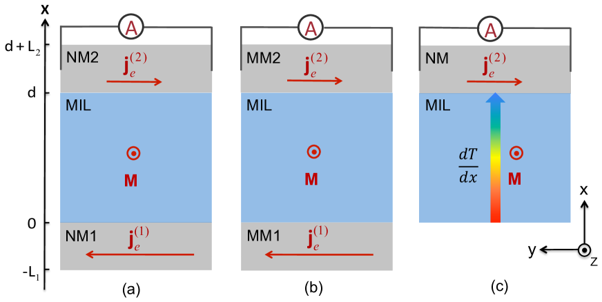
Figure 2: Schematics of three hypothetical devices: (a) NM$\mid$MIL$\mid$NM trilayers, (b) MM$\mid$MIL$\mid$MM trilayers, and (c) NM$\mid$MIL bilayers. In (a) and (b), a spin current is generated by an injected electric current via spin Hall effect, while in (c), a magnon current is induced by applying a thermal gradient. In all three cases, the magnetization directions of the MIL and the magnetic metal (MM) layers are oriented in $+z$.

IV.1 NM$\mid$MIL$\mid$NM trilayers

In Fig. 2(a), a magnetic insulator layer (MIL) is sandwiched between two non-magnetic metal (NM) layers. By applying an in-plane electrical current in the NM1 layer, a spin current flowing perpendicular to the layers would be generated due to the spin Hall effect. In this geometry, a partial spin current would flow into the MIL via transfer of spin current to magnon current. If the magnon diffusion length is larger than the thickness of the MIL, the magnon current would reach the other side of the MIL and subsequently, converts back to spin current in the NM2 layer. Finally, an electric current parallel to the layer is generated owing to the inverse spin Hall effect Saitoh06 . Such an electric drag phenomenon, namely, an electric current in one NM layer induces an electric current in the other when the two NM layers are separated by a MIL, would be a proof of the magnon/spin current conversion at magnetic interfaces. Although we have already calculated the drag coefficient in Ref. Zhang12 , we find the improved boundary conditions presented in this paper quantitatively modify the earlier result.

Referring to the coordinate system in Fig. 2, one can establish the relation of the spin accumulation, spin current, magnon accumulation, and magnon current in each layer. For the NM1 layer with an applied in-plane current density $j^{(1)}_{e}$, we have

$$\delta m_{s}(x)=A_{1}\exp(x/\lambda_{sf})$$ (14)

where $\lambda_{sf}$ is the spin diffusion length, $A_{1}$ is a constant to be determined via boundary conditions. We have taken the thickness of the layer much larger than the spin diffusion length such that the term proportional to $\exp(-x/\lambda_{sf})$ has been dropped. The spin current flowing perpendicular to the plane of the layers is given by

$$j^{(1)}_{s}(x)=-\gamma_{sh}j^{(1)}_{e}-D_{s}\frac{\partial\delta m_{s}}{\partial x}$$ (15)

where the first term represents the spin Hall effect: an electric current $j_{e}^{(1)}$ in the $y$-direction generates a transverse spin current proportional to the spin Hall angle $\gamma_{sh}$ which is defined as the ratio of the spin Hall conductivity to the electric conductivity. Note that we have adopted $e=\mu_{B}=1$ for notation convenience so that the electrical current and the spin current would have the same unit. The second term corresponds to the spin diffusion where $D_{s}$ is the spin diffusion coefficient which may be related to the conductivities $c_{\uparrow}=c_{\downarrow}$ by the Einstein relation: $c_{\uparrow(\downarrow)}=e^{2}g_{e}(\varepsilon_{F})D_{s}$. For the MIL layer, we have

$$\delta m_{m}(x)=A_{2}\exp(x/l_{m})+A_{3}\exp(-x/l_{m})$$ (16)

and

$$j_{m}(x)=-D_{m}\frac{\partial\delta m_{m}}{\partial x}$$ (17)

where $A_{2}$ and $A_{3}$ are integral constants from the magnon diffusion equation, $l_{m}$ is the magnon diffusion length, $D_{m}$ is the magnon diffusion constant associated with the magnon diffusion length by $l_{m}=\sqrt{D_{m}\tau_{th}}$ with $\tau_{th}$ being the magnon-nonconserving relaxation time Zhang12 . For the NM2 layer, we have

$$\delta m_{s}(x)=A_{4}\exp(x/\lambda_{sf})+A_{5}\exp(-x/\lambda_{sf})$$ (18)

and

$$j^{(2)}_{s}(x)=-D_{s}\frac{\partial\delta m_{s}}{\partial x}$$ (19)

where $A_{4}$ and $A_{5}$ are two integration constants. The four boundary conditions of Eqs. (2) and (3) at the two interfaces $x=0$ and $x=d$, along with the outer-boundary condition at $x=d+L_{2}$ where $j^{(2)}_{s}(x=d+L_{2})=0$, determine the five constants $A_{i}$ ($i=1-5$). After a straighforward algebra, we find the spin current density $j^{(2)}_{s}(x)$ which in turn converts to an in-plane charge current in the NM2 layer via the inverse spin Hall effect, i.e., $j_{e}^{(2)}(x)=\gamma_{sh}j^{(2)}_{s}(x)$. Explicitly,

$$j_{e}^{(2)}(x)=\frac{-ab\sinh\left[\frac{d+L_{2}-x}{\lambda_{sf}}\right]\mathrm{csch}\left(\frac{L_{2}}{\lambda_{sf}}\right)\gamma_{sh}^{2}j_{e}^{(1)}}{\left[b_{1}+b_{2}\coth\left(\frac{L_{2}}{\lambda_{sf}}\right)\right]\sinh\left(\frac{d}{l_{m}}\right)+\left[b_{3}+ab\coth\left(\frac{L_{2}}{\lambda_{sf}}\right)\right]\cosh\left(\frac{d}{l_{m}}\right)}$$ (20)

where we have introduced the dimensionless constants $a\equiv\lambda_{sf}G_{em}/D_{s}$, $b\equiv{l_{m}G_{me}}/D_{m}$ $b_{1}=1+a+b^{2}$, $b_{2}=a+a^{2}$, and $b_{3}=(2+a)b$. We may define an average electric current density by averaging over the thickness of the NM2 layer, $\bar{j}_{e}^{(2)}=(1/L_{2})\int dxj_{e}^{(2)}(x)$. Then the ratio of the averaged current density to the injected current density, i.e., $\eta\equiv\left|\bar{j}_{e}^{(2)}/j_{e}^{(1)}\right|$, can be obtained as

$$\eta=\frac{\lambda_{sf}\gamma^{2}_{sh}}{L_{2}}\frac{ab\tanh\left(\frac{L_{2}}{2\lambda_{sf}}\right)}{\left[b_{1}+b_{2}\coth\left(\frac{L_{2}}{\lambda_{sf}}\right)\right]\sinh\left(\frac{d}{l_{m}}\right)+\left[b_{3}+ab\coth\left(\frac{L_{2}}{\lambda_{sf}}\right)\right]\cosh\left(\frac{d}{l_{m}}\right)}$$ (21)

The electrical drag coefficient $\eta$ may be readily estimated. In the case of $d\ll l_{m}$, $\eta$ becomes independent of $G_{me}$, but increases with $G_{em}$; this is understandable since in this case the magnon current does not decay and thus the magnon accumulation is unimportant, $\eta$ depends predominantly on the efficiency of the magnon current generation by spin accumulation which is measured by $G_{em}$. A quick numerical check also indicates that $G_{em}$ is usually larger than $G_{me}$. We consider a trilayer of Ta$\mid$YIG$\mid$Ta whose material parameters at room temperature ($T=300K$) are taken as follows: for the Ta layers Buhrman12 , the conductivity $c_{Ta}=\left(190\mu\Omega\cdot cm\right)^{-1}$, the spin diffusion length $\lambda_{sf}=5$ $nm$ and the spin Hall angle $\gamma_{sh}=0.15$, the lattice constant $a_{0M}=3.3{\mathring{A}}$, and the Fermi energy $\varepsilon_{F}=5$ $eV$; for the YIG layer Callen65 , the Curie temperature $T_{c}=550$ $K$, the lattice constant $a_{0I}=12.376{\mathring{A}}$, the spin wave gap $\Delta_{g}=10^{-6}$ $eV$, and the magnon relaxation time $\tau_{th}=10^{-6}s$. In Fig. 3, we show $\eta$ as a function of the thicknesses of the NM2 layer for several different MIL thicknesses. Fig. 4 shows $\eta$ as a function of the interface exchange coupling $J_{sd}$ with several different magnon diffusion lengths.

Finally, we discuss the sign of the drag current. The induced electric current always flows in the opposite direction of the injected electric current for any magnetization direction of the MIL . To see this, we first recall the spin Hall and inverse spin Hall effect in a single layer: an electric current induces a perpendicular spin current (spin Hall) which in turn produces an electric current (inverse spin Hall). The physical principle is that the combined actions of the spin Hall and the inverse spin Hall are to reduce the original driving current. Now consider the trilayer system. Since the spin current injected into the NM2 layer remains parallel to the spin current in the NM1 layer, the electric drag current in the NM2 layer must be antiparallel to the applied electric current in the NM1 layer.

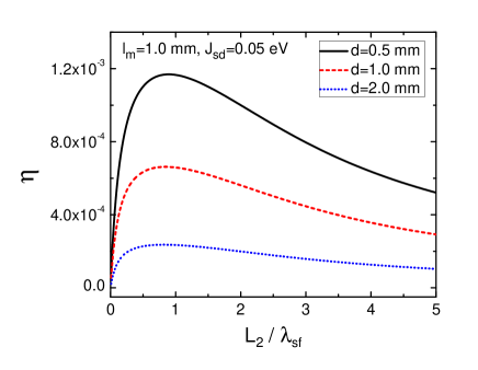
Figure 3: Electrical drag coefficient as a function of the NM2 (Ta) layer thickness for three different thicknesses of the MIL (YIG). See the main text for the parameters used in the figure.

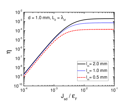
Figure 4: Electrical drag coefficient as a function of $J_{sd}/\varepsilon_{F}$ for three different magnon diffusion lengths of the MIL (YIG). See the main text for the parameters used in the figure.

IV.2 MM$\mid$MIL$\mid$MM trilayers

Next, we consider a trilayer structure where the two metallic layers are magnetic, as shown in Fig. 2(b). Since the direct contact between the magnetic metal (MM) layer and the MIL would make it difficult to rotate the magnetization of each layer independently, one may insert a thin non-magnetic layer at the interface to break direct magnetic coupling. When an in-plane current is applied to the MM1 layer, an anomalous Hall current perpendicular to the layers is generated if the magnetization is oriented in the $z$-axis. Although the physics of anomalous Hall and spin Hall effects are the same, the anomalous Hall current has both spin and charge currents. The charge current, however, is unable to penetrate the MIL; this leads to a charge accumulation at the interface so that the net charge current is exactly zero in the steady state. The spin current, on the other hand, is able to propagate into the MIL via the conversion to the magnon current, as discussed in the previous section. To gain a quantitative understanding, we carry out the following calculation.

The $x$-components of spin and charge currents of the MM1 layer can be expressed as

$$j_{s}^{x(1)}=-pD_{s}\frac{\partial\delta n_{0}^{(1)}}{\partial x}-D_{s}\frac{\partial\delta m_{s}^{(1)}}{\partial x}-\gamma_{ah}j_{e}^{(1)}$$ (22)

and

$$j_{e}^{x(1)}=-D_{s}\frac{\partial\delta n_{0}^{(1)}}{\partial x}-pD_{s}\frac{\partial\delta m_{s}^{(1)}}{\partial x}-p\gamma_{ah}j_{e}^{(1)}$$ (23)

where $p=(c_{\uparrow}-c_{\downarrow})/(c_{\uparrow}+c_{\downarrow})$ is the spin polarization of the conductivity, $\gamma_{ah}$ is the anomalous Hall angle defined as the ratio of the Hall conductivity to the longitudinal conductivity, $\delta n_{0}$ is the charge accumulation and $j_{e}^{(1)}$ is the current density applied in the $y$-direction as before. We have assumed a spin-independent spin diffusion coefficient $D_{s}$. Since $j_{e}^{x(1)}=0$, we may eliminate the charge accumulation term from Eq. (22) and get

$$j_{s}^{x(1)}=-(1-p^{2})D_{s}\frac{\partial\delta m_{s}^{(1)}}{\partial x}-(1-p^{2})\gamma_{ah}j_{e}^{(1)}$$ (24)

For the MIL, Eqs. (16) and (17) remain valid, while for the MM2 layer, we similarly have

$$j_{s}^{x(2)}=-(1-p^{2})D_{s}\frac{\partial m_{s}^{(2)}}{\partial x}$$ (25)

By comparing Eqs. (24) and (25) with Eqs. (15) and (19), one should realize that the induced electric current $j_{e}^{(2)}$ in the MM2 layer can be simply obtained by replacing $D_{s}$ by $(1-p^{2})D_{s}$ and $\gamma_{sh}$ by $(1-p^{2})\gamma_{ah}$ in Eq. (20). Consequently, the electrical drag current is reduced by a fact of $(1-p^{2})^{2}$ for the MM$\mid$MIL$\mid$MM trilayer if one approximates $\gamma_{sh}\approx\gamma_{ah}$. This might be counter-intuitive at first glance, since one would expect the magnetic metals to provide more spin signals. However, if we realize the interplay between the charge and spin currents, one can readily explain the above conclusion: consider the extreme case of $p=1$, i.e., spin current generated by the anomalous Hall is fully polarized such that the spin current is same as the charge current. Since the charge current is completely blocked by the MIL, it is inevitable that the spin current is also being completely blocked.

IV.3 NM$\mid$MIL bilayers

In this section, we consider a NM$\mid$MIL bilayer. In this case, the magnon current in the MIL is induced by a temperature gradient, see Fig. 2(c). From the magnon Boltzmann equation within the relaxation time approximation, the non-equilibrium magnon distribution is,

$$\delta N_{\mathbf{q}}=-v_{\mathbf{q}}^{x}\tau_{m}\frac{\partial N_{\mathbf{q}}^{0}}{\partial T}\frac{dT}{dx}-v_{\mathbf{q}}^{x}\tau_{m}\frac{\partial\delta N_{\mathbf{q}}}{\partial x}.$$ (26)

where $v_{\mathbf{q}}^{x}$ denotes the $x$-component of the magnon velocity and $\tau_{m}$ is the magnon-conserving relaxation time. By defining the magnon current as $j_{m}\equiv(2\mu_{B})\int d\mathbf{q}v^{x}_{\mathbf{q}}\delta N_{\mathbf{q}}$ and following the derivation in the Appendix A of the Supplemental Material of Ref. Zhang12 , we find

$$j_{m}=-\kappa\frac{dT}{dx}-D_{m}\frac{\partial\delta m_{m}}{\partial x}$$ (27)

with

$$\kappa=\frac{2\sqrt{3(S+1)}\mu_{B}\tau_{m}k_{B}^{2}T_{c}\xi}{9\pi\hbar^{2}a_{0I}}\left(\frac{T}{T_{c}}\right)^{\frac{3}{2}}$$ (28)

and $\xi=\int^{\infty}_{0}dxx^{3/2}e^{x}/(e^{x}-1)^{2}\simeq 3.4$. The magnon accumulation satisfies the magnon diffusion equation whose solution can be taken as a simple form,

$$\delta m_{m}(x)=B_{1}\exp(x/l_{m})$$ (29)

where we have assumed the thickness of the MIL to be much larger than the magnon diffusion length $l_{m}$ and hence dropped the term $\exp(-x/l_{m})$ in the solution. The spin accumulation in the NM layer can be written as

$$\delta m_{s}(x)=B_{2}\exp(x/\lambda_{sf})+B_{3}\exp(-x/\lambda_{sf})$$ (30)

and the spin current perpendicular to the plane is given by $j_{s}=-D_{s}\partial{\delta m_{s}}/{\partial x}$. These three integral constants $B_{i}$ ($i=1,2,3$) can be determined by the two interface boundary conditions Eqs. (2) and (3), along with the outer boundary condition $j_{s}(x=d+L_{2})=0$. After a straightforward algebra, we get

$$j_{s}(x)=\frac{b\kappa\sinh\left(\frac{d+L_{2}-x}{\lambda_{sf}}\right)}{(1+b)\sinh\left(\frac{L_{2}}{\lambda_{sf}}\right)+a\cosh\left(\frac{L_{2}}{\lambda_{sf}}\right)}\frac{dT}{dx}$$ (31)

Again, the above perpendicular-to-plane spin current can generate an in-plane electric current whose average density over the thickness of the NM layer can be obtained by $\bar{j}_{e}=(\gamma_{sh}/L_{2})\int j_{s}(x)dx$. By taking the temperature gradient as a constant, we have

$$\bar{j}_{e}=\frac{\lambda_{sf}}{L_{2}}\frac{\gamma_{sh}b\kappa\left[\cosh\left(\frac{L_{2}}{\lambda_{sf}}\right)-1\right]}{(1+b)\sinh\left(\frac{L_{2}}{\lambda_{sf}}\right)+a\cosh\left(\frac{L_{2}}{\lambda_{sf}}\right)}\frac{dT}{dx}.$$ (32)

The direction of the electric current is in the plane of the layer and perpendicular to the directions of the magnetization as well as the temperature gradient of the MIL. It is interesting to compare the current driven electric drag, Eq. (21), with the thermally driven electrical drag, Eq. (32). Firstly, in the former case, the electric drag is proportional to the square of the Hall angle because the first metallic layer converts the electric current to the spin current via spin Hall effect and the second metal layer converts the spin current into the electric current via inverse spin Hall effect, while in the latter case, the spin current is directly injected from the thermally driven magnon current and thus the drag current is linearly proportional to the spin Hall angle. Secondly, in the NM$\mid$MIL$\mid$NM case, both spin convertances $G_{em}$ and $G_{me}$ are important, while for NM$\mid$MIL, the convertance relating the magnon accumulation to the spin current, $G_{me}$, plays a dominant role. A rough estimation yields the induced current density in a Pt$\mid$YIG bilayer is about $10$ $A/cm^{2}$ for a moderately small temperature gradient of $dT/dx=10$ $K/cm$ if one chooses the following parameters: $\gamma_{sh}=0.05$ Buhrman11 , $J_{sd}=1$ $meV$, $L_{2}=\lambda_{sf}=7$ $nm$, $c_{Pt}=0.1$ $(\mu\Omega\cdot cm)^{-1}$, $a_{0M}=3.9$ ${\mathring{A}}$, $a_{0I}=12.376$ ${\mathring{A}}$, $\tau_{m}=10^{-8}$ $s$ Callen65 , $\tau_{th}=10^{-6}$ $s$, $l_{m}=1$ $mm$, $S=\frac{5}{2}$ and $T_{c}=550$ $K$.

V Discussions and Summary

We have investigated the spin transport across the interface between a metal layer and a MIL. The salient feature of our approach is that we have treated spin and magnon transport properties on an equal footing. Namely, the spin and magnon accumulations as well as the spin and magnon currents are described by semiclassical non-equilibrium distribution functions. In other approaches, for example, Xiao et al. Uchida10 ; Xiao10 described the magnon density through a quasi-equilibrium effective magnon temperature which differs from the lattice temperature. Adachi et al. Adachi11 ; Adachi12 considered the linear response theories and their numerical solutions Ohe on the spin Seeback effect Uchida10-nat ; Uchida10-APL in ferromagnetic insulators. These approaches also provide alternative physical insights on the roles of magnons in non-equilibrium transport Slonczewski10 .

We thank S. Bender for pointing out an inconsistency in the approximations used in the derivation of the spin convertance $G_{em}$ in a previous version of the paper. This work is supported by NSF-ECCS.

References

- (1) M. N. Baibich , J. M. Broto, A. Fert, F. Nguyen Van Dau, F. Petroff, P. Eitenne, G. Creuzet, A. Friederich, and J. Chazelas, Phys. Rev. Lett. 61, 2472 (1988).
- (2) G. Binasch, P. Grunberg, F. Saurenbach, and W. Zinn, Phys. Rev. B 39, 4828 (1989).
- (3) J. C. Slonczewski, J. Magn. Magn. Mater. 159, L1 (1996).
- (4) L. Berger, Phys. Rev. B 54, 9353 (1996).
- (5) J. E. Hirsch, Phys. Rev. Lett. 83 1834 (1999).
- (6) S. Zhang, Phys. Rev. Lett. 85, 393 (2000).
- (7) Y. Kajiwara et al., Nature 464, 262 (2010).
- (8) J. Xiao and G. E. W. Bauer, Phys. Rev. Lett. 108, 217204 (2012).
- (9) Z. Wang, Y. Sun, M. Wu, V. Tiberkevich, and A. Slavin, Phys. Rev. Lett. 107, 146602 (2011).
- (10) D. Hinzke and U. Nowak, Phys. Rev. Lett. 107, 027205 (2011).
- (11) P. Yan, X. S. Wang, and X. R. Wang, Phys. Rev. Lett. 107, 177207 (2011)
- (12) S. S.-L. Zhang and S. Zhang, Phys. Rev. Lett. 109, 096603 (2012).
- (13) T. Valet and A. Fert, Phys. Rev. B 48, 7099 (1993).
- (14) S. Zhang, P. M. Levy, A. C. Marley, and S. S. P. Parkin, Phys. Rev. Lett. 79, 3744 (1997).
- (15) S. Takahashi, E. Saitoh, and S. Maekawa, J. Phys.: Conference Series 200, 062030 (2010).
- (16) S. A. Bender, R. A. Duine, and Y. Tserkovnyak, Phys. Rev. Lett. 108, 246601 (2012).
- (17) E. Saitoh, M. Ueda, H. Miyajima, and G. Tatara, Appl. Phys. Lett. 88, 182509 (2006).
- (18) L. Liu, et al., Science 336, 555 (2012).
- (19) C. W. Haas and H. B. Callen, in Magnetism, Vol. I, edited by G. T. Rado and H. Suhl (Academic Press, New York, 1965).
- (20) L. Q. Liu, T. Moriyama, D. C. Ralph, and R. A. Buhrman, Phys. Rev. Lett. 106, 036601 (2011); a lower spin Hall angle for Pt was reported in Z. Feng et al., Phys. Rev. B 85, 214423 (2012).
- (21) K. Uchida et al., Nature Mater. 9, 894 (2010).
- (22) J. Xiao, G. E. W. Bauer, K. Uchida, E. Saitoh, and S. Maekawa, Phys. Rev. B 81, 214418 (2010).
- (23) H. Adachi, J. Ohe, S. Takahashi, and S. Maekawa, Phys. Rev. B 83, 094410 (2011).
- (24) H. Adachi and S. Maekawa, arXiv:1209.0228v1.
- (25) J. Ohe, H. Adachi, S. Takahashi, and S. Maekawa, Phys. Rev. B 83, 115118 (2011)
- (26) K. Uchida et al., Nature Mater. 9, 894 (2010).
- (27) K. Uchida et al., Appl. Phys. Lett. 97, 172505 (2010).
- (28) J. C. Slonczewski, Phys. Rev. B 82, 054403 (2010).