Why is the Milky Way $X$-factor Constant?

Abstract

The CO-H₂ conversion factor ($X_{\rm CO}$; otherwise known as the $X$-factor) is observed to be remarkably constant in the Milky Way and in the Local Group (aside from the SMC). To date, our understanding of why $X_{\rm CO}$ should be so constant remains poor. Using a combination of extremely high resolution ($\sim 1$ pc) galaxy evolution simulations and molecular line radiative transfer calculations, we suggest that $X_{\rm CO}$ displays a narrow range of values in the Galaxy due to the fact that molecular clouds share very similar physical properties. In our models, this is itself a consequence of stellar feedback competing against gravitational collapse. GMCs whose lifetimes are regulated by radiative feedback show a narrow range of surface densities, temperatures and velocity dispersions with values comparable to those seen in the Milky Way. As a result, the $X$-factors from these clouds show reasonable correspondence with observed data from the Local Group, and a relatively narrow range. On the other hand, feedback-free clouds collapse to surface densities that are larger than those seen in the Galaxy, and hence result in $X$-factors that are systematically too large compared to the Milky Way’s. We conclude that radiative feedback within GMCs can generate cloud properties similar to those observed in the Galaxy, and hence a roughly constant Milky Way X-factor in normal, quiescent clouds.

1 Introduction

Historically, determining H₂ gas masses in the interstellar medium (ISM) of galaxies has relied on the usage of tracer molecules. This owes to the fact that H₂ requires temperatures $\sim 500$ K to excite the rotational lines, and is thus a poor tracer of cold ($\sim 10-100$K) giant molecular clouds (GMCs). Carbon Monoxide (¹²CO; hereafter, CO) is the second most abundant molecule, and has strong lines in a readily accessible window of atmospheric transmission. For this reason, CO is the most commonly employed tracer of H₂. However, utilising CO as a measure of H₂ does not come without uncertainty.

At the heart of converting CO line fluxes to H₂ masses is the CO-H₂ conversion factor. The conversion factor relates either H₂ column densities to velocity-integrated CO line intensity ($X_{\rm CO}$; alternatively, the $X$-factor), or H₂ gas mass to CO line luminosity ($\alpha_{\rm CO}$). The two are related via $X_{\rm CO}$ (cm^-2/K-km s^-1) = $6.3\times 10^{19}\times\mbox{$\alpha_{\rm CO}$}$  (M_☉ pc^-2 (K-km s^-1)^-1). Uncertainties in CO abundances, H₂ gas fractions, and radiative transfer all complicate our understanding of $X_{\rm CO}$.

In principle, $X_{\rm CO}$ can be empirically calibrated with an independent measure of H₂ gas masses. Efforts along these lines have used CO line widths (combined with an assumption regarding the dynamical state of the GMC), dust mass measurements (combined with an assumed dust-to-gas ratio), or gamma-ray observations from GMCs to determine the CO-H₂ conversion factor (Larson, 1981; Solomon et al., 1987; Dickman, 1975; de Vries et al., 1987; Pineda et al., 2008; Leroy et al., 2011; Magdis et al., 2011; Bloemen et al., 1986; Strong & Mattox, 1996; Abdo et al., 2010; Delahaye et al., 2011). These measurements have all arrived at the conclusion that the $X$-factor in Milky Way GMCs is remarkably constant, displaying a relatively narrow range of $\mbox{$X_{\rm CO}$}\approx 2-4\times 10^{20}\mbox{cm${}^{-2}$/K-km s${}^{-1}$}$ ($\mbox{$\alpha_{\rm CO}$}\approx 3-6\ \mbox{\mbox{M${}_{\sun}$ }pc${}^{-2}$ (K-\mbox{km s${}^{-1}$})${}^{-1}$}$). Beyond this, observations of GMCs in relatively normal galaxies within the Local Group (that is, excluding the Small Magallenic Cloud; Leroy et al., 2011) have evidenced similar $X$-factors as in the Galaxy.

This said, not all galaxies exhibit $X$-factors comparable to the relatively constant Local Group disc galaxy value. In particular, heavily star-forming systems at low and high-$z$ appear to have $X$-factors roughly a factor 2-10 lower than the Milky Way average (e.g. Downes & Solomon, 1998; Tacconi et al., 2008; Meier et al., 2010; Narayanan, 2011), whereas low-metallicity galaxies can have $X$-factors up to a factor $\sim 100$ higher than the Galactic mean (e.g. Wilson, 1995; Arimoto et al., 1996; Israel, 1997; Boselli et al., 2002; Bolatto et al., 2008; Leroy et al., 2011; Genzel et al., 2012; Schruba et al., 2012). Critical questions include: (1) what is the origin of the nearly-constant $X$-factor in nearby disks, (2) why is $X_{\rm CO}$ depressed in high gas-surface density environments, and (3) why is the conversion factor elevated in low metallicity galaxies?

In recent years, there has been a flurry of interest from theorists in understanding $X_{\rm CO}$ on scales ranging from GMCs to cosmological simulations of galaxy formation. Models have made great headway in understanding the latter two questions. MHD calculations of evolving GMCs (Shetty et al., 2011a, b), cosmological galaxy formation calculations (Feldmann et al., 2012; Lagos et al., 2012) and hydrodynamic galaxy evolution calculations coupled with radiative transfer Narayanan et al. (2011b, 2012) have all converged on a picture in which low-metallicity galaxies have large fractions of CO-dark molecular gas (due to photodissociation of CO in regions of low dust extinction), and hence large $X_{\rm CO}$. Similarly, galaxy merger models by Narayanan et al. (2011b) and Narayanan et al. (2012) have shown that starburst environments can force large gas temperatures and velocity dispersions which increase the CO intensity at a given H₂ gas mass, thus reducing $X_{\rm CO}$.

This said, thus far no model that considers a full ensemble of clouds on galaxy-wide scales has been able to explain why the $X$-factor has such a narrow range of values in the Milky Way and nearby galaxies. To understand this requires knowledge of the physical state of GMCs on highly-resolved ($\sim$ pc) scales, but sampled over the scales of entire galaxies. That is, one ideally should be able to super-resolve GMCs while capturing the effect of the larger galactic environment on cloud evolution. Moreover, without explicit models for feedback, GMCs will inevitably collapse without limit (to arbitrarily high densities) and turn most of their mass into stars. This is in stark disagreement with observations indicating inefficient star formation and relatively short GMC lifetimes (e.g. Evans, 1999; Krumholz & Tan, 2007; Shirley et al., 2007; Kennicutt & Evans, 2012).

Recently, Hopkins et al. (2011) have implemented various forms of stellar feedback into idealised galaxy evolution simulations that have allowed for $\sim$ pc-scale resolution on galaxy-wide scales. These simulations move beyond previous models that employ subresolution assumptions governing molecular cloud evolution (e.g. Narayanan et al., 2011b, 2012) and allow us to super-resolve GMCs on galaxy-wide scales. These simulations have been utilised by Hopkins et al. (2012b) to show that a model in which radiative feedback from massive stars dominates the life-cycle of molecular clouds successfully reproduces many observed physical properties and scaling relations (e.g. “Larson’s Laws”) of GMCs, including their surface densities, velocity dispersions, size distributions and mass spectra. Here, we employ these simulations to model a Milky Way-like disc galaxy and ask whether GMCs whose physical properties are governed by radiative feedback can explain $X$-factor properties (i.e. their constancy) of observed Local Group GMCs.

2 Methods

We simulate the hydrodynamic evolution of a Milky Way-like galaxy with a substantially modified version of gadget-3, a smoothed-particle hydrodynamics (SPH) code (Springel et al., 2005; Springel, 2005). The main code modifications and model details are described in Hopkins et al. (2011, 2012b) and we describe only the important aspects here.

We initialise an exponential disc according to the Mo et al. (1998) model within a live dark matter halo of mass $1.6\times 10^{12}\mbox{M${}_{\sun}$ }$  with a Hernquist (1990) density profile and concentration parameter $c=12$. The baryon, bulge, disc and gas masses are initialised at ($M_{\rm bar},m_{b},m_{d},m_{g}$) = ($7.1,1.5,4.7,0.9$)$\times 10^{10}\mbox{M${}_{\sun}$}$, and scale-lengths ($h_{d},h_{g},z_{0}$)=$(3.0,6.0,0.3$) kpc. The simulations are run with $\sim 3\times 10^{7}$ hydrodynamic particles, with a smoothing length of $\sim 1$pc.

For the purposes of the SPH simulations, the gas is allowed to cool to $\sim 100$ K (though see below regarding further refinements on this temperature structure in post-processing), and the HI-H₂ balance is determined following the semi-analytic model of Krumholz et al. (2008, 2009). Stars form exclusively in H₂ gas that is self-gravitating on the smallest resolved scales. Stars form at an instantaneous rate of $\dot{\rho}_{*}=\rho/t_{\rm ff}(\rho)$; because feedback can prevent further star formation once stars form, the average efficiency of star formation in dense gas is typically $\sim 1\%$.

The most important aspect of the models is a range of mechanisms by which stellar feedback can impact the ISM. Throughout, we assume a Kroupa (2002) stellar IMF, and utilise starburst99 (Leitherer et al., 1999) for all stellar luminosity, mass return and supernova rate calculations as a function of stellar age and metallicity. The mechanisms of stellar feedback include:

1. Local Momentum Deposition: For the purposes of this work, the most important source of feedback is local momentum deposition by stellar radiation, mass return from stellar winds and supernova. At each timestep, the nearest density peak to a given gas particle is determined to represent a clump inside of a GMC. The total stellar radiation from all star particles inside a sphere defined by the distance between the gas particle and density peak are summed; the radiation from these stars is then used to determine the momentum flux.

   The momentum flux from radiation is given by $\dot{P}_{\rm rad}=(1+\tau_{\rm IR})\times(L/c)$, where $\tau_{\rm IR}=\Sigma_{\rm gas}\kappa_{\rm IR}$. $\Sigma_{\rm gas}$ is the gas surface density calculated directly from the simulation, and $\kappa_{\rm IR}$ is approximated by $\kappa_{\rm IR}=5(Z/Z_{\odot})$g^-1 cm².

   We also include direct momentum injection from SNe and stellar winds, whose momentum deposition rates are directly calculated from starburst99 and injected to the gas within a smoothing length of the star particle. This source of feedback is typically subdominant compared to radiation pressure in galaxies as massive as a MW analog.

2. Thermal Energy Input from Supernova and Stellar Wind Shock-Heating: For the supernovae (SNe), we tabulate Type I and II SNe rates from Mannucci et al. (2006) and starburst99, respectively, for all star particles and determine from a stochastic procedure if a SN occurred at each timestep. When a SN occurs, thermal energy is injected into the gas within a smoothing length of the star particle. For stellar winds, we inject the tabulated mechanical power as a function of stellar age and metallicity to the gas within a smoothing length of the star.

3. Photo-Heating of HII Regions The production rates of ionising photons from star particles is calculated and used to determine the extent of HII regions surrounding stars (allowing appropriately for overlapping regions). The temperatures of these HII regions are heated to $10^{4}$ K if the gas falls below that threshold.

4. Long-Range Radiation Pressure Photons that escape the local GMC (not accounted for in (i)), after being appropriately attenuated/absorbed, are propagated to large distances along direct rays, where local absorption is calculated by integrating over a frequency-dependent opacity (which also scales linearly with metallicity). The appropriate radiation pressure forces are then imparted.

Predicting the molecular emission requires calculating the correct temperature (including full radiative transfer effects) of molecular gas below $T=100\,$K (the approximate floor imposed by the cooling tables in the simulations). This is prohibitively expensive to perform on-the-fly, so in this paper we do so in post-processing. But we do not expect changes in the thermal pressure at such low temperatures to have any dynamical effect on the simulations. We calculate the temperature utilising the methodology described in Goldsmith (2001) and Krumholz et al. (2011b). The dominant heating processes of the H₂ gas are cosmic ray heating, the grain photoelectric effect, and dust-gas thermal exchange. The dominant cooling terms are cooling by CO, CII and dust. If the gas and dust are in thermal balance, then we have the following equations (where $\Gamma$ represents heating terms, and $\Lambda$ represents cooling terms):

$$\Gamma_{\rm pe}+\Gamma_{\rm CR}-\Lambda_{\rm line}+\Psi_{\rm gd}=0$$ (1)

$$\Gamma_{\rm dust}-\Lambda_{\rm dust}-\Psi_{\rm gd}=0$$ (2)

The equation is solved by simultaneously iterating on the temperatures of the gas and dust

We assume a Galactic cosmic ray heating rate and a grain photoelectric effect proportional to the local FUV intensity. We refer the reader to Krumholz et al. (2011a) for the specific values employed in the model. In short, however, the temperature can be thought of as density-dependent. At high densities ($n>10^{4}\mbox{cm${}^{-3}$}$), dust and gas exchange energy efficiently, and the gas temperature rises to the dust temperature. At low densities ($n<10^{2}\mbox{cm${}^{-3}$}$), cosmic rays dominate the heating. For a Milky Way cosmic ray flux, this corresponds to GMCs with temperatures $\sim 8-10$ K. Intermediate densities have temperatures in between the dust temperature and cosmic ray-determined temperature.

The dust temperature is calculated utilising sunrise, a publicly available Monte Carlo dust radiative transfer code (see Jonsson et al., 2010; Jonsson & Primack, 2010, for code descriptions, as well as Hayward et al. (2011, 2012a, 2012b) for further details). We utilise the simulation set-up described in Narayanan et al. (2011b), and refer the reader there for more details. In practice, the bulk of the gas remains below density $n=10^{4}\mbox{cm${}^{-3}$}$, the density at which dust-gas energy exchange becomes efficient.

The line cooling term is calculated in each cell via a 1D escape probability code (Krumholz & Thompson, 2007). We assume a fractional carbon abundance of $1.5\times 10^{-4}Z^{\prime}$, where $Z^{\prime}$ is the metallicity with respect to solar. The fraction of hydrogen where the carbon is in the form of CO is well approximated from both semi-analytic (Wolfire et al., 2010) and numerical models (Glover & Mac Low, 2011):

$$f_{\rm CO}=f_{\rm H2}\times e^{-4(0.53-0.045{\rm ln}\frac{G_{0}^{\prime}}{n_{\rm H}/{\rm cm^{-3}}}-0.097{\rm ln}Z^{\prime})/A_{\rm v}}$$ (3)

where $G_{0}^{\prime}$ is the FUV intensity relative to the Solar neighbourhood. Physically, Equation 3 describes the photodissociation of CO from UV photons, and its ability to survive behind sufficient columns of dust. When $f_{\rm CO}>0.5$, we assume that CO dominates the line cooling; else, CII.

Finally, we note that we do not explicitly include the effects of heating by turbulent dissipation. In Narayanan et al. (2011b), we performed tests in which the contribution of viscous dissipation and adiabatic compression to the turbulent heating rate were included in the model. These tests showed that, for quiescent discs, this source of heating only affects the final temperature by a few percent.

With the physical and chemical state of the molecular gas known, we utilize turtlebeach, a 3D non-local thermodynamic equilibrium adaptive mesh Monte Carlo line radiative transfer code to calculate the velocity integrated CO line intensity (Narayanan et al., 2006, 2008, 2011a, 2011b). We refer the reader to Narayanan et al. (2011b) for the formal equations, and only summarise the relevant points here.

CO line emission is set by the level populations. The source function for a given transition $u\rightarrow l$ is given by:

$$S_{\nu}=\frac{n_{u}A_{ul}}{(n_{l}B_{lu}-n_{u}B_{ul})}$$ (4)

where $A_{ul},B_{lu}$ and $B_{ul}$ are the Einstein rate coefficients, and $n$ are the level populations.

We first calculate the level populations within a given cell utilising the escape probability formalism (Krumholz & Thompson, 2007). We emit model photons from each cell isotropically with emission frequency drawn from a Gaussian profile function. When the photon passes through a cell, it sees an opacity of:

$$\alpha_{\nu}^{ul}(\rm gas)=\frac{h\nu_{ul}}{4\pi}\phi(\nu)(\it n_{l}B_{lu}-n_{u}B_{ul})$$ (5)

where $\nu$ is the transition frequency, and $\phi(\nu)$ is the line profile function that takes into account the effects of line of sight velocity offsets in the opacity.

Once the model photons have all been emitted, the level populations are updated by assuming detailed balance (Narayanan et al., 2011b). The collisional rate coefficients are taken from the Leiden Atomic and Molecular Database (Schöier et al., 2005). This process is iterated upon until the level populations are converged to $<1\%$ across all cells.

GMCs within the model are identified via a friends of friends finder with a linking length of $20\%$ of the mean cell size. Tests have shown that the results are not substantially sensitive to this choice.

3 Why is the X-factor Constant?

To first order, $X_{\rm CO}$ can be thought of as the column density of GMCs divided by the product of their temperature and velocity dispersion. Formally, $X_{\rm CO}$= $N_{\rm H2}/W_{\rm CO}$, where $W_{\rm CO}$ is the velocity-integrated CO intensity. When the gas is in local thermodynamic equilibrium (as CO J=1-0 almost always is), the amplitude of the emission line is proportional to the gas kinetic temperature $T_{\rm K}$. Similarly, because CO (J=1-0) is typically optically thick within GMCs, increasing the velocity dispersion of the gas increases the emergent CO intensity. As a result, $W_{\rm CO}$ increases for both increasing kinetic temperature, as well as increasing velocity dispersion. So, to ask why the $X$-factor in MW GMCs is nearly constant is to ask why observed gas temperatures, velocity dispersions, and surface densities have a narrow distribution of values.

3.1 The Physical Properties of GMCs in Galaxy Discs

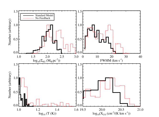
Figure 1: Mass-weighted distributions over all GMCs of gas surface density, velocity dispersion, temperature, and $X$-factor for our fiducial model (solid black line), and a feedback-free model (dotted line). Feedback-free GMCs collapse to higher surface densities than models that include feedback, driving more power into large $X_{\rm CO}$ values.

In Figure 1, we show the mass-weighted distributions of GMC temperatures, velocity dispersions, surface densities, and $X$-factors for our fiducial MW model at a randomly chosen time snapshot (though the results are consistent for the bulk of the galaxy’s evolution). As we will see, the physical properties of the GMCs are generally determined by the radiative feedback that eventually disrupts the GMC.

In our model disc, the GMCs can be thought of as roughly isothermal, with temperatures $\sim 10$ K. The average densities of the GMCs are relatively low, with $n\approx 10-100\ \mbox{cm${}^{-3}$}$. At these densities, the gas is energetically decoupled from the dust, and cosmic rays act as the primary heating source. For a Galactic cosmic ray flux (which we assume), this equates to a minimum gas temperature of roughly $\sim 10$ K. We note that this is in reasonable agreement with measurements from the Milky Way. For example, the mass-weighted mean temperature for all GMCs in the Solomon et al. (1987) First Quadrant survey is $\sim 11.3$ K. If we restrict the averaging to only GMCs with reported temperatures $T>10K$ to avoid any potentially subthermally excited clouds, the mass weighted average temperature is $\sim 13$K. Both values are in good agreement with our modeled values in Figure 1.

The GMC surface densities display a range of values centred around $\sim 100\ \mbox{$\mbox{M${}_{\sun}$ }{\rm pc}^{-2}$}$. We calculate the surface density as $\Sigma_{\rm H2}=M/(\pi\times R_{\rm C}^{2})$, where the radius of the GMC ($R_{\rm C}$) is half the average of the maximum length in three orthogonal directions. While this is method is not free of geometric effects, it is a reasonable approximation to the methods used in observations. These surface densities are comparable to collapse conditions for gas that forms GMCs. In a model where the GMC lifetime is regulated by radiative feedback, GMCs do not collapse indefinitely. Once GMCs reach surface densities near 100 $\mbox{M${}_{\sun}$ }{\rm pc}^{-2}$, feedback from star formation disperses the cloud. These surface densities are not far from the average value of the disc, as the model GMC only lives a few $\times 10^{6}$ yr (e.g. a few free fall times). Beyond this, these surface densities are comparable to those seen in Galactic GMCs, which display a relatively narrow range (Larson, 1981; Solomon et al., 1987; Heyer et al., 2009, though see Lombardi et al. (2010)).

It is worth noting here that the $X$-factor is implicitly dependent on the volumetric density of the GMCs residing within a range of $n\sim 50-10^{4}$ cm^-3. At larger densities, the gas and dust exchange energy efficiently, and the gas temperature rises to that of the dust temperature (Goldsmith, 2001; Krumholz et al., 2011b), driving it to larger values than the roughly $\sim 10$ K value seen when cosmic rays dominate the heating. At lower densities, the CO may not be in LTE (depending on the degree of line radiative trapping). In this regime, the peak CO intensity will no longer scale with the kinetic temperature of the gas. As in the case with the GMC surface densities, radiative feedback suppresses the formation of excessive amounts of dense gas (Hopkins et al., 2012a). The median density of GMCs is $\sim 100$ cm^-3, and the distribution within the galaxy is roughly lognormal in shape.

The GMCs in these simulations are consistent with being marginally gravitationally bound (Hopkins et al., 2012b), and have velocity dispersions ranging from a few to $\sim 20$ km s^-1. Disruption of the GMC by radiative feedback keeps the GMC from becoming too strongly self-gravitating, and hence limits the velocity dispersions. Comparing these to the typical velocity dispersion of GMCs seen in the Galaxy (Solomon et al., 1987), the range of modeled GMC velocity dispersions is reasonable.

3.2 $X$-factor properties in Galaxy discs

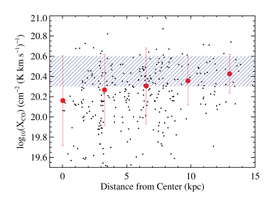
Figure 2: $X$-factors  of model GMCs in our fiducial model galaxy as a function of galactocentric distance. Black circles represent the individual GMCs, while the red filled circles denote the median of all GMCs within bins of $\sim$ 3 kpc (with the dispersion within the bin shown as error bars). The blue shaded region shows the rough range of values for the Milky Way. GMCs toward the centre of the galaxy tend to have lower $X$-factors due to systematically larger velocity dispersions, though the trend is relatively weak, and there is significant dispersion.

We can now see why the $X$-factor is relatively constant in Milky Way-like disc galaxies. If the evolution of GMCs is largely governed by radiative feedback, their surface densities and velocity dispersions display a relatively narrow range of values comparable to measurements of Galactic GMCs. If, beyond this, the temperatures of GMCs are nearly isothermal at $\sim 10$ K, as expected for clouds where the dominant heating source is cosmic rays with a flux comparable to the Galaxy’s, then the CO-H₂ conversion factor will display a relatively narrow range of values centred around 2-4 $\times 10^{20}$  cm^-2/K-km s^-1. We see this in the fourth panel of Figure 1.

In Figure 2, we show the relationship between $X_{\rm CO}$ in our model GMCs and their distance from the centre of the galaxy. The black points denote the individual GMCs, while the red circles and error bars denote the median and dispersion within roughly 3 kpc bins. The blue shaded region shows the average Galactic range for the $X$-factor. Generally, GMCs toward the centre of the model Milky Way analog systematically have lower $X$-factors than clouds at larger distances from the galactic centre. Influenced by a large stellar potential, as well as other gas, GMCs toward the centre of the galaxy tend to have larger velocity dispersions than field GMCs, and tend to be unvirialised. There is some tentative observational evidence that $X_{\rm CO}$ values in GMCs decrease from the Galactic mean toward the centre of the Milky Way (Oka et al., 1998; Strong et al., 2004), as well as in other nearby galaxies (Sandstrom et al., 2012). This said, there is significant dispersion in observed trends of $X_{\rm CO}$ with galactic radius, and some observations show nearly no depression at all (less than a factor of 2) toward galactic nuclei (Donovan Meyer et al. in prep.).

The $X$-factor from our model GMCs compares well to the observed population of GMCs within the Galaxy. In the left panel of Figure 3, we show the virial masses of observed GMCs in the Galaxy and NGC 6946 against their CO luminosities from Solomon et al. (1987) and Donovan Meyer et al. (2012). We additionally show the $M_{\rm vir}-L_{\rm CO}$ relation for our model galaxies. We defer discussion of the right panel for § 3.3. The normalisation of the $M_{\rm vir}-L_{\rm CO}$ relation in the model GMCs (black solid points), which betrays the conversion of CO to H₂ gas mass, corresponds reasonably well with the observed data (red stars). This is shown more explicitly in the left panel of Figure 4, which shows the relationship between $\alpha_{\rm CO}$ and cloud virial mass for both observed and modeled GMCs.

Figure 3: Virial mass versus CO luminosity for observed GMCs (red stars), and modeled clouds (black filled circles). Left plot shows our fiducial galaxy, and right plot a feedback-free model. While the clouds in our fiducial galaxy show excellent correspondence with observed GMCs, the feedback-free clouds systematically has $X$-factors that are too large, driving the simulated $M_{\rm vir}-L_{\rm CO}$ relation a factor of a few higher than the observed points.

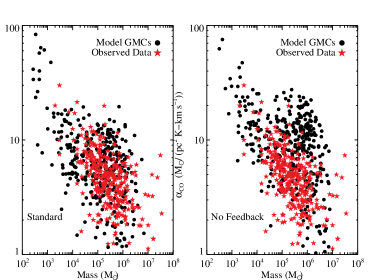
Figure 4: $\alpha_{\rm CO}$ ($M$/L_CO) as a function of cloud virial mass. Symbols are as in Figure 3. While the typical range of modeled CO-H₂ conversion factors in our fiducial model correspond well with observations, the feedback-free model systematically has conversion factors that are too large.

3.3 Feedback-Free Models

In order to highlight the role of feedback in setting the physical properties of the model GMCs, it is worth considering the properties of a feedback-free model. At this point, we now highlight the dotted red line in Figure 1, which denotes a model run with exactly the same initial conditions as our fiducial model, though with no forms of feedback included. When GMCs first form, their properties are not especially different in models with and without feedback, as expected from general models of gravitational instability and fragmentation (Hopkins, 2011). But GMCs in models without feedback proceed to collapse one-dimensionally, developing a pancake-shaped geometry and spinning up (Hopkins et al., 2012b). While the general surface density distribution is not terribly dissimilar from our fiducial model, feedback-free GMCs develop a large tail of very high-density gas, and show more power toward large $\Sigma_{\rm H2}$. The velocity dispersion distribution additionally increases moderately (due to a spinning up of the contracting GMC), as well as the temperature (due to more gas at or above the gas-dust coupling density of $\sim 10^{4}\mbox{cm${}^{-3}$}$), but these increases are more modest than the increase in the GMC surface densities.

The net result of feedback-free GMCs is more power toward large $X$-factors, and typical $X$-factors a factor $\sim 2-3$ larger than typical MW GMCs. As an example, in the right panel of Figure 3, we plot the $M_{\rm vir}-L_{\rm CO}$ relation for observed GMCs and model GMCs in a feedback-free model. Compared to our standard model, which shows excellent correspondence with observed data, the feedback-free model lies a factor of a few above the $M_{\rm vir}-L_{\rm CO}$ relation. The right panel of Figure 4 further empahsises this point by showing the relationship between modeled conversion factors from feedback-free GMCs, and observed ones for Galactic clouds. Beyond this, as noted by Hopkins et al. (2012b), feedback-free models exhibit a host of problems, including star formation rates well above the observed Kennicutt-Schmidt relation, gas density distributions (and HCN/CO line ratios) above those observed (Hopkins et al., 2012a), and abnormally low virial parameters.

3.4 Summary

Utilising a combination of high-resolution galaxy evolution simulations that super-resolve giant molecular clouds and 3D molecular line radiative transfer calculations, we investigate why the CO-H₂ conversion factor ($X_{\rm CO}$) is observed to be roughly constant in the Milky Way and Local Group galaxies (aside from the SMC).

Our main result is that $X_{\rm CO}$ is found to be nearly constant because all GMCs in our model Milky Way have similar physical conditions to one another. In particular, $X_{\rm CO}$ is determined principally by GMC surface densities, temperatures, and velocity dispersions.

• The model GMCs all have similar surface densities at values near $\sim 100\ \mbox{$\mbox{M${}_{\sun}$ }{\rm pc}^{-2}$}$. Models that include radiative feedback limit GMCs from achieving surface densities much larger than this value due to cloud dispersal.

• The temperatures of GMCs are dominated by cosmic ray heating. Given a Milky Way cosmic ray flux, this results in nearly isothermal GMCs with temperatures $\sim 8-10$ K.

• The GMCs in our model are consistent with being marginally bound, resulting in a narrow velocity dispersion range of $5-20$ km s^-1.

These GMCs display a relatively narrow range of physical properties, and compare well with those observed in the Milky Way. As a result, the CO-H₂ conversion factor in these clouds additionally shows a narrow range of values. Feedback is a necessary element in the model to control the cloud surface densities, and hence limit the observed range of $X_{\rm CO}$. Feedback-free models collapse to large surface densities, and hence show excessive power to large $X_{\rm CO}$ values.

References

- Abdo et al. (2010) Abdo, A. A. et al. 2010, ApJ, 709, L152
- Arimoto et al. (1996) Arimoto, N., Sofue, Y., & Tsujimoto, T. 1996, PASJ, 48, 275
- Bloemen et al. (1986) Bloemen, J. B. G. M., Strong, A. W., Mayer-Hasselwander, H. A., Blitz, L., Cohen, R. S., Dame, T. M., Grabelsky, D. A., Thaddeus, P., Hermsen, W., & Lebrun, F. 1986, A&A, 154, 25
- Bolatto et al. (2008) Bolatto, A. D., Leroy, A. K., Rosolowsky, E., Walter, F., & Blitz, L. 2008, ApJ, 686, 948
- Boselli et al. (2002) Boselli, A., Lequeux, J., & Gavazzi, G. 2002, AP&SS, 281, 127
- de Vries et al. (1987) de Vries, H. W., Thaddeus, P., & Heithausen, A. 1987, ApJ, 319, 723
- Delahaye et al. (2011) Delahaye, T., Fiasson, A., Pohl, M., & Salati, P. 2011, A&A, 531, A37+
- Dickman (1975) Dickman, R. L. 1975, ApJ, 202, 50
- Donovan Meyer et al. (2012) Donovan Meyer, J., Koda, J., Momose, R., Fukuhara, M., Mooney, T., Towers, S., Egusa, F., Kennicutt, R., Kuno, N., Carty, M., Sawada, T., & Scoville, N. 2012, ApJ, 744, 42
- Downes & Solomon (1998) Downes, D. & Solomon, P. M. 1998, ApJ, 507, 615
- Evans (1999) Evans, II, N. J. 1999, ARA&A, 37, 311
- Feldmann et al. (2012) Feldmann, R., Gnedin, N. Y., & Kravtsov, A. V. 2012, ApJ, 747, 124
- Genzel et al. (2012) Genzel, R. et al. 2012, ApJ, 746, 69
- Glover & Mac Low (2011) Glover, S. C. O. & Mac Low, M.-M. 2011, MNRAS, 412, 337
- Goldsmith (2001) Goldsmith, P. F. 2001, ApJ, 557, 736
- Hayward et al. (2012a) Hayward, C. C., Jonsson, P., Kereš, D., Magnelli, B., Hernquist, L., & Cox, T. J. 2012a, MNRAS, 424, 951
- Hayward et al. (2011) Hayward, C. C., Kereš, D., Jonsson, P., Narayanan, D., Cox, T. J., & Hernquist, L. 2011, ApJ, 743, 159
- Hayward et al. (2012b) Hayward, C. C., Narayanan, D., Kereš, D., Jonsson, P., Hopkins, P. F., Cox, T. J., & Hernquist, L. 2012b, arXiv/1209.2413
- Hernquist (1990) Hernquist, L. 1990, ApJ, 356, 359
- Heyer et al. (2009) Heyer, M., Krawczyk, C., Duval, J., & Jackson, J. M. 2009, ApJ, 699, 1092
- Hopkins (2011) Hopkins, P. F. 2011, arXiv/1111.2863
- Hopkins et al. (2012a) Hopkins, P. F., Narayanan, D., Murray, N., & Quataert, E. 2012a, arXiv/1209.0459
- Hopkins et al. (2011) Hopkins, P. F., Quataert, E., & Murray, N. 2011, MNRAS, 417, 950
- Hopkins et al. (2012b) —. 2012b, MNRAS, 421, 3488
- Israel (1997) Israel, F. P. 1997, A&A, 328, 471
- Jonsson et al. (2010) Jonsson, P., Groves, B. A., & Cox, T. J. 2010, MNRAS, 186
- Jonsson & Primack (2010) Jonsson, P. & Primack, J. R. 2010, New Astronomy, 15, 509
- Kennicutt & Evans (2012) Kennicutt, Jr., R. C. & Evans, II, N. J. 2012, arXiv/1204.3552
- Kroupa (2002) Kroupa, P. 2002, Science, 295, 82
- Krumholz et al. (2011a) Krumholz, M. R., Dekel, A., & McKee, C. F. 2011a, arXiv/1109.4150
- Krumholz et al. (2011b) Krumholz, M. R., Leroy, A. K., & McKee, C. F. 2011b, ApJ, 731, 25
- Krumholz et al. (2008) Krumholz, M. R., McKee, C. F., & Tumlinson, J. 2008, ApJ, 689, 865
- Krumholz et al. (2009) —. 2009, ApJ, 693, 216
- Krumholz & Tan (2007) Krumholz, M. R. & Tan, J. C. 2007, ApJ, 654, 304
- Krumholz & Thompson (2007) Krumholz, M. R. & Thompson, T. A. 2007, ApJ, 669, 289
- Lagos et al. (2012) Lagos, C. d. P., Bayet, E., Baugh, C. M., Lacey, C. G., Bell, T., Fanidakis, N., & Geach, J. 2012, arXiv/1204.0795
- Larson (1981) Larson, R. B. 1981, MNRAS, 194, 809
- Leitherer et al. (1999) Leitherer, C. et al. 1999, ApJS, 123, 3
- Leroy et al. (2011) Leroy, A. K., Bolatto, A., Gordon, K., Sandstrom, K., Gratier, P., Rosolowsky, E., Engelbracht, C. W., Mizuno, N., Corbelli, E., Fukui, Y., & Kawamura, A. 2011, ApJ, 737, 12
- Lombardi et al. (2010) Lombardi, M., Alves, J., & Lada, C. J. 2010, A&A, 519, L7
- Magdis et al. (2011) Magdis, G. E., Daddi, E., Elbaz, D., Sargent, M., Dickinson, M., Dannerbauer, H., Aussel, H., Walter, F., Hwang, H. S., Charmandaris, V., Hodge, J., Riechers, D., Rigopoulou, D., Carilli, C., Pannella, M., Mullaney, J., Leiton, R., & Scott, D. 2011, ApJ, 740, L15
- Mannucci et al. (2006) Mannucci, F., Della Valle, M., & Panagia, N. 2006, MNRAS, 370, 773
- Meier et al. (2010) Meier, D. S., Turner, J. L., Beck, S. C., Gorjian, V., Tsai, C., & Van Dyk, S. D. 2010, AJ, 140, 1294
- Mo et al. (1998) Mo, H. J., Mao, S., & White, S. D. M. 1998, MNRAS, 295, 319
- Narayanan (2011) Narayanan, D. 2011, arXiv/1112.1073
- Narayanan et al. (2011a) Narayanan, D., Cox, T. J., Hayward, C. C., & Hernquist, L. 2011a, MNRAS, 412, 287
- Narayanan et al. (2008) Narayanan, D., Cox, T. J., Kelly, B., Davé, R., Hernquist, L., Di Matteo, T., Hopkins, P. F., Kulesa, C., Robertson, B., & Walker, C. K. 2008, ApJS, 176, 331
- Narayanan et al. (2011b) Narayanan, D., Krumholz, M., Ostriker, E. C., & Hernquist, L. 2011b, MNRAS, 418, 664
- Narayanan et al. (2012) Narayanan, D., Krumholz, M. R., Ostriker, E. C., & Hernquist, L. 2012, MNRAS, 421, 3127
- Narayanan et al. (2006) Narayanan, D., Kulesa, C. A., Boss, A., & Walker, C. K. 2006, ApJ, 647, 1426
- Oka et al. (1998) Oka, T., Hasegawa, T., Hayashi, M., Handa, T., & Sakamoto, S. 1998, ApJ, 493, 730
- Pineda et al. (2008) Pineda, J. E., Caselli, P., & Goodman, A. A. 2008, ApJ, 679, 481
- Sandstrom et al. (2012) Sandstrom, K. M. et al. 2012, arXiv/1212.1208
- Schöier et al. (2005) Schöier, F. L., van der Tak, F. F. S., van Dishoeck, E. F., & Black, J. H. 2005, A&A, 432, 369
- Schruba et al. (2012) Schruba, A., Leroy, A. K., Walter, F., Bigiel, F., Brinks, E., de Blok, W. J. G., Kramer, C., Rosolowsky, E., Sandstrom, K., Schuster, K., Usero, A., Weiss, A., & Wiesemeyer, H. 2012, arXiv/1203.4321
- Shetty et al. (2011a) Shetty, R. et al. 2011a, MNRAS, 412, 1686
- Shetty et al. (2011b) —. 2011b, MNRAS, 415, 3253
- Shirley et al. (2007) Shirley, Y. L., Wu, J., Bussmann, R. S., & Wootten, A. 2007, arXiv/0711.4605, 711
- Solomon et al. (1987) Solomon, P. M., Rivolo, A. R., Barrett, J., & Yahil, A. 1987, ApJ, 319, 730
- Springel (2005) Springel, V. 2005, MNRAS, 364, 1105
- Springel et al. (2005) Springel, V., Di Matteo, T., & Hernquist, L. 2005, MNRAS, 361, 776
- Strong & Mattox (1996) Strong, A. W. & Mattox, J. R. 1996, A&A, 308, L21
- Strong et al. (2004) Strong, A. W., Moskalenko, I. V., Reimer, O., Digel, S., & Diehl, R. 2004, A&A, 422, L47
- Tacconi et al. (2008) Tacconi, L. J. et al. 2008, ApJ, 680, 246
- Wilson (1995) Wilson, C. D. 1995, ApJ, 448, L97+
- Wolfire et al. (2010) Wolfire, M. G., Hollenbach, D., & McKee, C. F. 2010, ApJ, 716, 1191