Chromospheric Thermal Continuum Millimetre Emission from non-dusty K and M Red Giants

Abstract

We examine the thermal free-free millimetre fluxes expected from non-dusty and non-pulsating K through mid-M giant stars based on our limited understanding of their inhomogeneous chromospheres. We present a semi-analytic model that provides estimates of the radio fluxes for the mm wavelengths (e.g., CARMA, ALMA, JVLA Q-band) based on knowledge of the effective temperatures, angular diameters and chromospheric Mg II h & k emission fluxes. At 250 GHz, the chromospheric optical depths are expected to be significantly less than unity, which means that fluxes across the mm and sub-mm range will have a contribution from the chromospheric material that gives rise to the ultraviolet emission spectrum, as well as the cool molecular material known to exist above the photosphere. We predict a lower bound to the inferred brightness temperature of red giants based on heating at the basal-flux limit if the upper chromospheres have filling factor $\simeq 1$. Multi-frequency mm observations should provide important new information on the structuring of the inhomogeneous chromospheres, including the boundary layer, and allow tests of competing theoretical models for atmospheric heating. We comment on the suitability of these stars as mm flux calibrators.

1 Introduction

Convective motions beneath the photospheres of late-type (cool) stars agitate the plasma, leading to the excitation of acoustic and magnetic disturbances. These waves induce non-radiative heating of the upper photosphere and chromosphere. Essentially all cool stars possess material heated above the prediction of radiative equilibrium, which emits a chromospheric spectrum that is most conspicuous in the ultraviolet (uv). The specific roles of acoustic and magnetic waves in heating the quiet solar chromosphere and the role of magnetic fields in structuring its atmosphere are the subject of considerable debate (Kalkofen, Ulmschneider, & Avrett, 1999; Ayres, 2002; Vecchio, Cauzzi, & Reardon, 2009). For the Sun and red giants the chromospheric plasma has a detectable signature in the millimetre (mm) thermal continuum (Altenhoff, Thum, & Wendker, 1994; Loukitcheva, Solanki, Carlsson, & Stein, 2004).

Stellar chromospheric surface fluxes measured from dominant emission lines, such as Ca II H & K and Mg II h & k, show a wide scatter at a given effective temperature ($T_{\rm eff}$), just as found for regions of different activity on the Sun. However, there is a well defined empirical lower bound known as the basal-flux, which is a strong function of effective temperature, $F_{\rm basal}\sim T_{\rm eff}^{7}$, but is only a weak function of surface gravity ($g_{\ast}$). The chromospheric cooling from the quietest solar regions, in the centres of supergranules, is close to the basal-flux for a $T_{\rm eff}=5770$ K star (e.g., Schrijver & Zwaan 2000). Stars that have chromospheric emission above the basal-flux are thought to have additional contributions from areas of enhanced surface magnetic activity, analogous to solar active regions (sunspots and associated plage). However, no consensus has been reached about the origin of the basal-flux. One line of thought is that it arises from the deposition of purely acoustic shock energy generated in the sub-photospheric convection zone (Ulmschneider, 1991), while the absence of appropriate spectroscopic shock signatures in inactive basal-flux red giants (Judge & Carpenter, 1998) suggests a magnetic origin. In fact, on the Sun both mechanisms are seen to operate: small-scale transient shock heating in the so-called ”K grains” and more steady magnetic heating in the large-scale supergranulation network.

The physical structures of chromospheres from these two mechanisms are likely to be quite different. The acoustic wave picture would lead to a 3-D network of shocks that is highly time variable and at a given position the gas temperature would fluctuate from very cool to very hot with the mean temperature being cool (Wedemeyer-Böhm et al., 2007). This mechanism leads to localized intermittent chromospheric emission but, which when averaged over the stellar disk, would not be apparent in the mm-radio. The presence of magnetic fields can lead to longer lived structures and enhanced atmospheric heating. Time-independent 1-D semi-empirical models for the Sun that represent regions of different activity are well established (Vernazza et al. 1976, 1981; Fontenla et al. 1990). Similar but spatially unresolved models have been constructed for a few cool stars including inactive red giants. These semi-empirical models are designed to reproduce the temporally and spatially averaged uv and optical emission line profiles and fluxes. A characteristic of these models is that they require a gradual temperature rise from the top of the photosphere to the upper chromosphere, and then a very steep rise through the chromosphere-coronae transition region (Kelch et al., 1978; Harper, 1992; Luttermoser et al., 1994; McMurry, 1999).

One might expect that acoustic models, whose mean temperatures do not increase with height, would fail to predict the same uv fluxes as semi-empirical models with an outward temperature increase, but this is not necessarily the case. In the uv, $h\nu/kT\gg 1$ and the source functions and emissivity $\propto e^{-h\nu/kT}$ are very sensitive to temperature. In this situation, the shock peaks can dominate the temporally and spatially averaged emission of the dynamic atmosphere. Thus it is possible for acoustic shock and semi-empirical models to produce the same chromospheric fluxes even though the temperature structures are profoundly different (Carlsson & Stein, 1995).

However, in the mm-radio, the thermal continuum source (Planck) function depends linearly on $T_{\rm e}$, so both solar and stellar mm observations can probe differences between intermittent and long-term structured atmospheres and potentially differentiate between acoustic and magnetically heating models. A comparison between uv and radio diagnostics could test the symbolic inequality

$$\langle e^{-h\nu/kT}\rangle\neq e^{-h\nu/k\langle T\rangle}$$ (1)

where the averages are over space and time. The LHS exemplifies uv emission diagnostics while the RHS reflects the same source function but with the mean temperature, $\langle T\rangle$, as inferred for example from mm radio emission. In practice uv and mm-radio fluxes calculated from different atmospheric models can be compared to observations. The hydrogen ionization determines the electron densities which, in part, determine both the mm-radio opacity and the uv collisional excitation rates. The remaining difference in the temperature dependence for formation leads to the test of equation (1).

Here we analyze published thermal mm (250 GHz) fluxes (Altenhoff et al., 1994) from single non-dusty and non-pulsating K and M giants (luminosity class III) to investigate their chromospheric signatures and explore the role of future multi-frequency observations in revealing the nature of chromospheric structuring. Future solar Atacama Large Millimeter/submillimeter Array (ALMA)imaging will be focussed on obtaining sufficient spatial resolution to separate the magnetic and non-magnetic regions (Loukitcheva et al., 2008), whereas studies of inactive basal-flux red giants may allow us to avoid the contamination from magnetic active regions by observing giants that are covered with inactive chromospheric regions analogous to quiet solar supergranule centres.

A first estimate for the expected mm flux from a red giant is provided by the hard disk model; which is appropriate when the ionized density scale height, $H^{\rm ion}_{\rho}$ is much smaller than the stellar radius, $R_{\ast}$. The observed flux density ($F_{\nu}$) is given by

$$F_{\nu}=\left(\phi/2\right)^{2}F_{\nu}^{\ast},$$ (2)

where $F_{\nu}^{\ast}$ is the average flux density at the surface, having angular diameter $\phi$ with respect to the distance observer. Working in terms of brightness temperatures $T_{\rm Br}$ we have

$$F_{\nu}={\pi k\nu^{2}\phi^{2}\over{2c^{2}}}\int\limits_{0}^{1}T_{\rm Br}\left(\mu\right)\mu\>d\mu={\pi k\nu^{2}\phi^{2}\over{c^{2}}}\langle T_{\rm Br}\rangle$$ (3)

where $\mu$ is the usual cosine of the angle between a ray and the normal to the emitting surface, and $\langle T_{\rm Br}\rangle$ is the weighted mean brightness temperature. In more convenient units, the flux in mJy is

$$F_{\nu}\left({\rm mJy}\right)=13.8\left({\langle T_{\rm Br}\rangle\over{3900\>{\rm K}}}\right)\left({\nu\over{250\>{\rm GHz}}}\right)^{2}\left({\phi\over{10\>{\rm mas}}}\right)^{2}$$ (4)

Many nearby red giants now have measured angular diameters, $\phi_{\ast}$, and estimated effective temperatures, $T_{\rm eff}$ (Mozurkewich et al., 2003). Inserting $\phi_{\ast}$ and substituting $T_{\rm eff}$ for $\langle T_{\rm Br}\rangle$ into equation (4) shows that many of these giants can in principle be observed at multiple frequencies with high signal-to-noise ratios when ALMA is completed given the expected sensitivity limits (Butler & Wooten, 1999). Here we develop a more physically motivated semi-analytical model for mm fluxes that incorporates constraints on chromospheric structure from independent IR and uv observations, which also allows us to include the effects of different levels of chromospheric heating.

In §2 we compile pertinent empirical constraints derived from semi-empirical models and other studies of red giants; and in §3 estimate the expected chromospheric mm optical depths. In §4 we develop a semi-analytic model for $\langle T_{\rm Br}\rangle$ based on these empirical constraints, which we then calibrate against direct measurements of the well studied red giant $\alpha$ Tau (K5 III) (Aldebaran). A comparison with observations and specific predictions for ALMA frequencies are presented in §5, and a discussion of the diagnostic potential of mm observations in §6. Conclusions are drawn in §7.

2 Empirical Constraints on Stellar Chromospheres

In this section we gather together nuggets of information from previous studies of red giant chromospheres, which we will incorporate into our analytic model for the mm radio fluxes. The radio optical depth, $\tau_{\nu}$, is proportional to different powers of the atmospheric properties - electron density, temperature, and path length - and we seek to estimate these for stars covering a range of $T_{\rm eff}$ and different levels of stellar activity.

Historically, the usual lack of temporal and spatial resolution in observations of the chromospheres of distant stars partly motivated the development of 1-D time-independent semi-empirical models. The earliest models used diagnostics observable from the ground – Ca II H & K, the Ca II IR triplet, and H$\alpha$ – and early satellite observations of Mg II h & k from Copernicus (Ayres et al., 1974; Ayres & Linsky, 1975). These types of models are analogous to the venerable VAL series of solar models, although for the latter spatial resolution did permit construction of components representative of regions of different activity levels (Vernazza et al., 1976, 1981). More recent variants of these solar component models are the FAL series (Fontenla et al., 1990), which are employed in solar irradiance studies (Fontenla et al., 2009), among other uses. Two notable features of these semi-empirical models are: (1) the temperature inversion in the low chromopshere above a temperature minimum, $T^{\rm uv}_{\rm min}\simeq 0.75T_{\rm eff}$; and (2) that the electron density, $n_{\rm e}$, is, to within a factor of $\sim 2$, approximately constant throughout the chromosphere (Ayres, 1979; Harper, 1992). At the temperature minimum, the electron density ($\sim 10^{-4}n_{\rm H}$) is dominated by (photo)ionized metals; but as the temperature increases through the chromosphere, hydrogen gradually becomes more ionized until at the top of the chromosphere ($\sim 10^{4}$ K), hydrogen is predominantly ionized and then $n_{\rm e}\sim n_{\rm H}$.

Thus, through the chromosphere, the increasing ionization of hydrogen counteracts the rapid outward decline of the density due to hydrostatic equilibrium, maintaining a more-or-less constant $n_{e}$ with increasing altitude (Ayres, 1979). However, once the hydrogen has become mostly ionized, there no longer is a ready source of bound electrons to be liberated, and so in the higher layers the electron density will fall off rapidly, following the hydrostatic decline in $n_{\rm H}$ itself (Ayres, 1979).

While there is a debate on whether the Sun has a permanent chromospheric temperature rise or not - it should be noted that presently the semi-empirical models nevertheless are the best thermodynamic inventory of stellar chromospheric plasma available. They approximately reproduce the amounts of plasma at different electron temperatures. This is discussed further in §6.

Pre-IUE, Mg II h & k observations revealed a strong dependence of chromospheric heating with effective temperature, $F_{\rm MgII}^{\ast}\sim T_{\rm eff}^{6}$ (Linsky & Ayres, 1978; Ayres, 1979). Ayres (1979) developed a scaling law for the mass column density at the onset of the chromospheric temperature rise, which can be rephrased in terms of the chromospheric electron density, $n_{\rm e}$, where atmospheric heating is sufficient to overcome $H^{-}$ cooling, namely

$$n_{e}\sim{\cal A}_{\rm Fe}^{1/2}{\cal F}^{1/2}g_{\ast}^{1/2}T_{\rm eff}^{5/2}.$$ (5)

${\cal A}_{\rm Fe}$ represents the abundance of low first ionization potential elements relative to solar, ${\cal F}$ is the possible enhancement of a particular star relative to the general $T_{\rm eff}$ scaling related to differences in intrinsic activity. In Ayres (1979), ${\cal F}=1$ was taken to represent levels appropriate to inactive stars or the quiet sun, and ${\cal F}=10$ for solar plage regions or (fast rotating) stars showing enhanced activity. Some empirical evidence for this trend on $n_{\rm e}$ in red giants is given by Byrne et al. (1988) based on IUE C II] 2325 Å intersystem flux ratios, and by Buchholz et al. (1998) who compared time-dependent acoustically heated atmospheric models with the mass column density of an effective $T^{\rm uv}_{\rm min}$. Chromospheric mm radio fluxes are sensitive to the opacity, which in turn depends on the square of the electron density. Here we assume the scaling in equation (5) provides an appropriate dependence of $n_{\rm e}$ on star specific parameters.

2.1 Basal Fluxes

We begin by considering the ratio of a star’s measured Mg II h & k flux to the basal-flux, i.e., a basal-flux star has ${\cal F}=1$. We recall the usual implicit assumption that Mg II h & k line fluxes represent a fixed fraction of the total chromospheric radiative losses (Linsky & Ayres, 1978). The other major coolants are H Ly$\alpha$, Ca II, and Fe II (e.g., Judge & Stencel 1991).

For this work we take IUE Mg II h & k fluxes from Martínez et al. (2011), which have typical uncertainties of $\pm 10$%, and we also adopt their $V-K$-based expression for the basal-flux (erg cm${}^{2}\>{\rm s}^{-1}$),

$$\log{F_{\rm basal}}=6.78\log{T_{\rm eff}}-19.74$$ (6)

which has a very similar $T_{\rm eff}$-dependence to Linsky & Ayres (1978). We have chosen specifically their $V-K$ form of the basal-flux, because the implied angular diameters are more reliable than the $B-V$ form at lower $T_{\rm eff}$. Judge & Stencel (1991) presented Mg II h & k surfaces fluxes for a sample of low and intermediate mass giants, and their lower-bound drops below equation (6) for $T_{\rm eff}<3300$ K.

2.2 Inhomogeneous Chromospheres

Observations of the $4.6\mu$m CO fundamental bands have demonstrated that on the Sun and late-type stars there exist regions of cool molecular gas with temperatures well below the $T^{\rm uv}_{\rm min}$ derived from ultraviolet and optical diagnostics (Ayres & Testerman, 1981; Wiedemann et al., 1994). On the sun the area filling factor of the CO material has been proposed to be up to 80% in the low chromosphere (Ayres, 2002), but that factor is controversial. For the red giants the filling factor is close to unity with the temperature scaling as $T_{\rm CO}\sim 0.60T_{\rm eff}$ (which is close to radiative equilibrium values when molecular cooling is included). At present there is a vigorous debate as to the exact nature of the CO clouds given the highly dynamic, time-dependent nature of the solar atmosphere (Kalkofen, Ulmschneider, & Avrett, 1999; Ayres, 2002; Leenaarts, Carlsson, Hansteen, & Gudiksen, 2011). The presence of the CO material must be accounted for in chromospheric models, particularly when these regions are probed by mm continuum emission. For example, recent spectral interferometry of the much later spectral-type M giant BK Vir (M7 III) has revealed the presence of spatially extended CO with an inner extended component at $R=1.2R_{\ast}$, with $T_{\rm CO}\simeq 0.65T_{\rm eff}$ (Ohnaka et al., 2012).

At lower effective temperatures, other molecules, such as water vapour (Tsuji, 2008), can play a role in further reducing the effective boundary layer temperature. Quirrenbach et al. (1993) found evidence from the Mark III interferometer that the TiO continuum becomes significantly geometrically extended by M5 III (R Lyr), for which the ratio of TiO to continuum diameters is $1.12\pm 0.02$. These extended molecular components possibly are related to the ‘molsphere phenomenon’ that is more common in the Mira and lower gravity M stars (Tsuji et al., 1997; Perrin et al., 2004).

2.3 Chromospheric Extent

The apparent angular size of a stellar radio source clearly is an important determinant of the radio flux. Here we consider the factors that control the angular diameter in the mm band, and in particular its ratio, $G$, to the photospheric angular diameter, i.e., $\phi_{\rm mm}=G\phi_{\ast}$.

The ratio of pressure scale-height, $H_{\rm pres}$, to stellar radius, $R_{\ast}$, is

$${H_{\rm pres}\over{R_{\ast}}}\sim{T_{\rm eff}R_{\ast}\over{M_{\ast}}},$$ (7)

so that red giants with their much larger radii, but near solar masses, have relatively thicker chromospheres than the Sun.

Eclipse observations of the $\zeta$ Aurigae systems, which have intermediate mass K Ib primaries, show large plasma turbulence and direct evidence for atmospheric extensions greater than the thermal pressure scale height, (e.g., Eaton 1993). This indicates that $H_{\rm pres}$ is controlled by both thermal and non-thermal motions. Here we describe the increase in $H_{\rm pres}$ from non-thermal flows by a quasi-hydrostatic equilibrium,

$$H_{\rm pres}={v^{2}+2kT\over{2\langle\mu\rangle m_{\rm H}kg_{\ast}}},$$ (8)

where $v$ is a characteristic velocity. For $\zeta$ Aur systems, $v$ is consistent with the turbulence inferred from spectra, and possibly correlated on spatial scales comparable to the density/pressure scale-height. $\langle\mu\rangle$ is the chromospheric average of the mean mass per particle in units of the hydrogen mass $m_{\rm H}$, and $g_{\ast}$ is the surface gravity. We adopt $\langle\mu\rangle=1.2$ corresponding to a partially ionized hydrogen ($n_{\rm e}\simeq 0.1n_{\rm H}$) and surface helium abundance of $n_{\rm He}=0.1n_{\rm H}$. Semi-empirical models typically include this non-thermal term in the equations of quasi-hydrostatic equilibrium. For $\zeta$ Aur systems, the implied turbulence is slightly greater than the hydrogen sound speed, and in our model we set $v=\sqrt{2kT}$. While estimates of stellar radii are available from interferometry (e.g., Baines et al. 2010) and nearby red giants also have Hipparcos parallaxes, the stellar masses remain uncertain for the single stars. Typical estimates are $1-2M_{\odot}$, leading to some uncertainty in the surface gravity in equation (8).

The semi-empirical one-component model of $\alpha$ Tau (McMurry, 1999) predicts a 250 GHz (1.2 mm) radial optical depth of unity at $R\simeq 1.03R_{\ast}$, but the apparent angular diameter (half central intensity) corresponds to $\phi_{\rm mm}\simeq 1.1\phi_{\ast}$. This is a result of the larger column density of the tangential sight-lines that define the 1.2 mm limb. The apparent angular diameter of $\alpha$ Boo predicted from a semi-empirical model of (Drake, 1985) is $\phi_{\rm mm}\simeq 1.06\phi_{\ast}$, and for g Her (M6 III) $\phi_{\rm mm}\simeq 1.08\phi_{\ast}$ (Luttermoser et al., 1994). These models were constructed with different diagnostics and assumptions about the contribution of turbulent pressure. So although there is a trend of increasing fractional chromospheric extension with later spectral type, the lower $T_{\rm eff}$ and thus lower chromospheric heating, leads to lower $n_{\rm e}$ and reduced mm-optical thickness. In light of these competing factors we adopt a typical extension of $1.08\phi_{\ast}$ (i.e., $G=1.08$), and accept an additional uncertainty of $\sim 2\%$ in $G$ which is consistent with the level of approximations adopted here. In summary, here $\langle T_{\rm Br}\rangle$ for the mm radio is defined as

$$\langle T_{\rm Br}\rangle={2c^{2}F_{\nu}\over{\pi k\nu^{2}\left(G\phi_{\ast}\right)^{2}}}$$ (9)

Very recently, single baseline, spectrally-resolved, K giant chromospheric Ca II IR-triplet visibilities from CHARA have been presented by Berio et al. (2011). The authors attempted to estimate the chromospheric extent by using a correction procedure based on the Eriksson et al. (1983) semi-empirical chromosphere of the coronal star $\beta$ Cet (K0 III). Berio et al. (2011) derive chromospheric extents of $1.16-1.47R_{\ast}$, although these values are based on a model whose actual spatial extent is only $1.02R_{\ast}$. The extended emission observed in the cores of the IR-triplet lines depends on the presence of Ca II ions which might not be related to the regions of higher electron density to which the radio is sensitive. The calculation of the IR-triplet visibilities requires a careful treatment of the Ca II to Ca III photoionization by H Ly$\alpha$ (Linsky & Avrett, 1970; Rowe, 1992), spherical geometry, and possible impact of cross-redistribution of photons scattering within the Ca II H & K resonance lines (Uitenbroek, 1989). The new CHARA measurements are very important diagnostics and one of us (NO’R) is undertaking these non-LTE radiative transfer calculations at the present time.

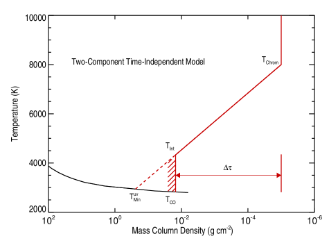
Figure 1: Schematic diagram of an idealized static two-component inhomogeneous red giant chromosphere. The warm chromosphere temperature rises outwards from $T_{\rm Int}$ to $T_{\rm Chrom}$ and had a total optical thickness $\Delta\tau$. Beneath the warm component, lies an opaque cool molecular region with $T_{\rm CO}<T^{\rm uv}_{\rm Min}$.

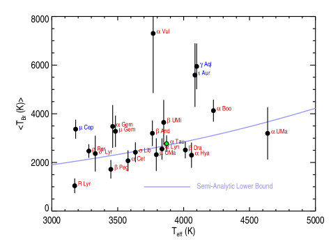
Figure 2: 250 GHz brightness temperatures for the sample given in Table 1. We also show three additional stars ($\mu$ Cep, $\iota$ Aur, and $\gamma$ Aql) which are of higher luminosity and might have emission in excess to that predicted by our model. The basal $\langle T_{\rm Br}\rangle$ predicted from our model is also shown as a solid curve.

3 Chromospheric millimetre optical thickness

As mentioned earlier the chromospheric electron density has contributions from the low first ionization potential elements and from hydrogen. At low temperatures ($T<6000~{}K$), ionization of hydrogen is a two stage process: excitation to the $n=2$ level by electron collisions or scattered H Ly$\alpha$ photons followed by photoionization by the optically thin photospheric Balmer continuum. At higher temperatures, direct collisional ionization becomes important. When hydrogen is partially ionized, free-free (thermal bremsstrahlung) opacity dominates at mm wavelengths. To examine the influence of the stellar outer atmosphere on the mm thermal emission, we first consider the optical thickness of the warm chromospheric component. For typical conditions, the opacity corrected for stimulated emission is given by Rybicki & Lightman (2004)

$$\kappa={0.01772\>n_{\rm e}n_{\rm ion}Z_{\rm ion}^{2}\over{T_{\rm e}^{1.5}\nu^{2}}}g_{\rm ff}\>\>{\rm cm}^{-1}$$ (10)

where the variables are in cgs units, $Z_{\rm ion}$ is the charge of the ions, $n_{\rm e}$ and $n_{\rm ion}$ are the number densities of the electrons and ions, respectively, and $g_{\rm ff}$ is the free-free Gaunt factor. At cm-wavelengths the familiar power-law approximation from Altenhoff et al. (1960) is

$$g^{\rm cm}_{\rm ff}=11.96T_{\rm e}^{+0.15}\nu^{-0.1},$$ (11)

but at ALMA frequencies,which range from 84-950 GHz (Band 3-10), the power-law dependence is slightly different, namely

$$g^{\rm sub-mm}_{\rm ff}=24.10T_{\rm e}^{+0.26}\nu^{-0.17},$$ (12)

as derived using the accurate Gaunt factors from Hummer (1988). Under typical chromospheric conditions, the majority of abundant species are either neutral or single ionized so that $Z_{\rm ion}=1$ and $n_{\rm e}=n_{\rm ion}$. This leads to an expression for the mm opacity,

$$\kappa_{\nu}={0.427n_{\rm e}^{2}\over{T_{\rm e}^{1.24}\nu^{2.17}}}\>\>{\rm cm}^{-1}$$ (13)

The optical thickness of a slab of depth, $\Delta L$, is then simply $\Delta\tau_{\nu}=\kappa_{\nu}\Delta L$.

The assumption that the electron density is approximately constant, as the ionization $n_{\rm e}/n_{\rm H}$ goes from $10^{-4}\to 1$, implies that the hydrogen density has declined by four orders of magnitude and therefore the physical thickness of the layer $\Delta L\simeq 9$ density scale-heights. To the level of approximation here we set $H_{\rho}\simeq H_{\rm pres}$

For the radial optical depth of the chromosphere we have

$$\Delta\tau_{\nu}\simeq{0.427\>n_{\rm e}^{2}\over{T_{\rm e}^{1.24}\nu^{2.17}}}\cdot 9\cdot{2kT_{\rm e}\over{\langle\mu\rangle m_{\rm H}g_{\ast}}}\simeq{6.4\>n_{\rm e}^{2}\over{T_{\rm e}^{0.24}\nu^{2.17}}}{k\over{m_{\rm H}g_{\ast}}}$$ (14)

This expression reveals only a very weak dependence on temperature variations within the chromosphere which is a result of the cancellation resulting from the combination of opacity and scale-height. In the following, we set the surviving temperature factor to $T_{\rm eff}^{0.24}$. Inserting into equation (14) typical values for the M2.5 III star $\beta$ Peg (Decin et al. 2003: $M_{\ast}=2.0M_{\odot}$, $R=110R_{\ast}$, $T_{\rm eff}=3600$ K) and a typical uv-based value of $n_{\rm e}\sim 6\times 10^{8}\>{\rm cm}^{-3}$ (Byrne et al., 1988), we find for 1.2 mm (250 GHz) and 3 mm (100 GHz) chromospheric optical thicknesses of $\Delta\tau_{{\rm 250GHz}}\simeq 0.1$ and $\Delta\tau_{{\rm 100GHz}}\simeq 0.8$, respectively. Thus depending on the level of stellar activity, the mm wavelength regime is one where chromospheres can go from optically thick at mm and cm wavelengths to optically thin in the sub-mm.

If the optical thickness of the chromosphere is less than unity the next emitting layer we must consider is the cool molecular gas immediately above photosphere with its near unity filling factor. In these cool, high density layers, where the hydrogen density increases rapidly with depth, H^- free-free can become an important opacity source (Harper et al., 2001). Here we assume that the bifurcated molecular regions are opaque at these wavelengths. Thus the optical depth unity is reached when $T_{\rm e}\simeq T_{\rm CO}$, which is reasonable if the temperatures in these outer radiative equilibrium layers change only slowly with optical depth.

Table 1: Adopted properties of $\alpha$ Tau.

Quantity	Value	Unit	Reference
Spectral Type		K5 III
$\phi_{\ast}$	$21.1\pm 0.2$	mas	Mozurkewich et al. (2003)
$T_{\rm eff}$	$3871\pm 48$	K	ditto
$R_{\star}$	$44.56\pm 2.94$	$R_{\odot}$	Decin et al. (2003)
$\log{g_{\ast}}$	$1.5\pm 0.15$	${\rm cm\>s}^{-2}$	ditto
$M_{\star}$	$2.30\pm 0.85$	$M_{\odot}$	inferred ($g_{\star}$)
[Fe/H]	$-0.15\pm 0.20$		ditto
$F_{\rm Mg~{}II}(h+k)$	$6.50\times 10^{4}$	${\rm erg\>cm}^{-2}{\rm s}^{-1}$	Martínez et al. (2011)+$\phi_{\ast}$
$F_{\rm Mg~{}II}/F_{\rm basal}$	1.69		ditto

4 Description of the Semi-Analytic Model

We now assemble the different aspects discussed above and construct a semi-analytic model to provide estimates of the mm, e.g., ALMA band, radio fluxes. We then calibrate against well studied $\alpha$ Tau (K5 III) to normalize all the approximation constants of order unity accumulated along the way. A schematic representation of the model inhomogeneous chromosphere is shown in Figure 1. Above the uv temperature minimum $T_{\rm Min}^{\rm uv}$ lies the opaque cool molecular material with temperature $T_{\rm CO}$. Immediately above this, perhaps in an overlying magnetic canopy, is the base of the warm chromosphere with temperature $T_{\rm Int}$; $T_{e}$ then rises linearly in mass column density to the upper chromosphere with temperature $T_{\rm Chrom}$ and has an optical thickness $\Delta\tau$. In the model $n_{\rm e}$ is approximately constant (to within a factor of $\pm 2$) and $T_{\rm e}$, in the warm component, is approximately linear with height. The source function $S_{\nu}\propto T_{\rm e}$, and since the mm optical depth is $\tau_{\nu}\propto n_{\rm e}^{2}\Delta L$, then $S_{\nu}$ is a linear function of $\tau_{\nu}$. In this case the integration of the formal solution of the radiative transfer equation for the brightness temperature can be done analytically.

$T_{\rm Br}$, a function of frequency and viewing angle, represents a weighted contribution of the three temperature parameters and is given by

$$T_{\rm Br}\left(\mu\right)=\alpha T_{\rm CO}+\gamma T_{\rm Int}+\beta T_{\rm Chrom}$$ (15)

where $T_{\rm CO},T_{\rm Int},T_{\rm Chrom}$ are the key temperatures described above and weighting coefficients are obtained from the formal solution of the transfer equation (Olson & Kunasz, 1987), which in our notation are

$$\alpha=e^{-\Delta\tau}$$ (16)

$$\beta=1-\left(1-\alpha\right)/\Delta\tau$$ (17)

$$\gamma=1-\alpha-\beta.$$ (18)

From Wiedemann et al. (1994) we adopt $T_{\rm CO}\simeq 0.6T_{\rm eff}$ and $T_{\rm Int}=4500$ K. We take $T_{\rm Chrom}=10000$ K where hydrogen has become 50% ionized (McMurry, 1999) and any further increase in temperature now leads to a rapid decline in $n_{\rm e}$ and hence also $\kappa_{\nu}$, creating a transparent boundary above $T_{\rm Chrom}$.

In this analytic model, the radio fluxes are dependent on $T_{\rm eff}$ and the optical depth of the warm chromosphere layer above the CO zone. If the emitting layers are not too thick compared to the stellar radius, the stellar flux can be described as the integral of $T_{\rm Br}\left(\mu\right)$ for a plane-parallel slab, where $\mu=\cos\theta$ and $\theta$ is the angle between the atmosphere normal and the ray. This allows us to write a weighted mean brightness temperature, e.g., in equation (4), as

$$\langle T_{\rm Br}\rangle = 2\int\limits_{0}^{1}T_{\rm Br}\left(\mu\right)\mu\>d\mu$$ (19)

$$= 2\sum\limits_{i=1}^{n}T_{\rm Br}\left(\mu_{i}\right)\mu_{i}w_{i}=T_{\rm Br}\left(\mu=1/2\right)$$ (20)

In keeping with the simple nature of our analytic model we replaced the integral by a single point Gaussian quadrature ($n=1$, $\mu_{1}=1/2$, and $w_{1}=1$). $\langle T_{\rm Br}\rangle$ is found by substituting $\Delta\tau$ from equation (14), adjusted for the viewing angle $\mu=1/2$, into equations (16), (17), and (18) to evaluate the weighting coefficients and then solve for equation (15).

4.1 Calibrating with $\alpha$ Tau (K5 III)

To mitigate some of the inherent uncertainties in the model we evaluate the chromospheric optical thickness (equation 14) for $\alpha$ Tau using empirical constraints. We initially use the scheme outlined above to calculate the 250 GHz flux and compare it to the measured 1986 IRAM Altenhoff et al. (1994) flux of $51\pm 6$ mJy. $\Delta\tau$ then is scaled by a constant to normalize the model. We use the Altenhoff et al. (1994) compilation because it represents the largest stellar sample available. We later (§5.3) compare $\alpha$ Tau to more recent interferometric observations by Cohen et al. (2005).

Robinson, Carpenter, & Brown (1998) give estimates of $n_{\rm e}$ in $\alpha$ Tau for three epochs (1990, 1994, and 1996) based on near-uv C II spectra obtained with the Hubble Space Telescope: $n_{\rm e}\simeq 10^{9}\>{\rm cm}^{-3}$. Unfortunately there were no contemporaneous IUE observations in 1986 when the IRAM 250 GHz observations were made. Electron densities inferred from the C II] 2325 Å multiplet ratios are weighted towards regions of high $T_{\rm e}$ and $n_{\rm e}$. Because semi-empirical models show that $n_{\rm e}$ is constant to within a factor of $\sim 2$, we adopt a mean $n_{\rm e}$ that is half the peak observed value, $<n^{2}_{\rm e}>=n^{2}_{\rm e}(HST)/4$.

The predicted flux is then obtained from equation (3) with $G=1.08$ and $\langle T_{\rm Br}\rangle$ given by the model. Combining the stellar parameters adopted in Table 1, we derive $F_{\rm 250GHz}=52$ mJy, likely a fortuitous agreement. The model predicts a radial optical depth of $\Delta\tau_{\mu=1}=0.05$ and $\Delta\tau_{\mu=1/2}=0.09$.

4.2 Star to star variations in $\Delta\tau$

$\alpha$ Tau’s Mg II h & k flux is about 1.7 times basal, and it might be slightly metal poor (see Tables 2 and 1, respectively) both of which affect the optical thickness. To scale this chromospheric thickness to other red giants, and remove explicit dependence on $\alpha$ Tau’s stellar parameters, we define an optical thickness $\Delta\tau_{\nu}\left(\mu\right)$ for a fictitious star with $\alpha$ Tau’s $T_{\rm eff}$ but now with basal-flux heating (${\cal F}=1$) and solar metalicity. Using the Ayres (1979) scaling of equation (5) gives $\Delta\tau_{\mu=1}^{\rm basal}=0.04$.

Combining equation (5) and equation (6), the chromospheric optical thickness becomes

$$\Delta\tau_{\nu}^{\ast}\left(\mu\right)={0.04\over{\mu}}{A_{\rm Fe}\over{A_{\rm Fe\odot}}}{F_{\ast}\over{F_{\rm basal}}}\left({T_{\rm eff}\over{3871\>{\rm K}}}\right)^{5.54}\left({\nu\over{250\>{\rm GHz}}}\right)^{-2.17}.$$ (21)

Note that the surface gravity term has now cancelled.

Table 2: Stellar properties, 250 GHz radio fluxes, and chromospheric optical thicknesses. The stellar properties are from Mozurkewich et al. (2003), the mm fluxes, except $\sigma$ Lib, are from Altenhoff et al.(1994) and the Mg II fluxes are from Martinez et al. (2011).

Star	HR	HD	Spectral	$T_{\rm eff}$	$\sigma(T_{\rm eff})$	$\phi$	$\sigma(\phi)$	$Flux$	$\sigma(Flux)$	$F/F_{\rm basal}$	$\Delta\tau$
			Type	$(K)$	$(K)$	$(mas)$	$(mas)$	(mJy)	(mJy)	(Mg II h & k)	($\mu=1/2$)
$\beta$ And	337	6860	M0 III	3763	46	13.75	0.14	25.0	4.0	2.2	0.15
$\alpha$ Cet	911	18884	M1.5 IIIa	3578	53	13.24	0.26	15.0	3.0	2.0	0.10
$\rho$ Per	921	19058	M4 II	3281	40	16.55	0.17	28.0	3.0	1.7	0.05
$\alpha$ Tau	1457	29139	K5 III	3871	48	21.10	0.21	51.0	6.0	1.7	0.09
$\iota$ Aur	1577	31398	K3 II	4086	50	7.50	0.07	13.0	3.0	1.7	0.18
$\eta$ Gem	2216	42995	M3 III	3462	43	11.79	0.12	20.0	5.0	3.0	0.13
$\mu$ Gem	2286	44478	M3 IIIab	3483	43	15.12	0.15	31.0	6.0	1.3	0.06
$\alpha$ Lyn	3705	80493	K7 III	3836	47	7.54	0.07	6.0	1.0	1.9	0.14
$\alpha$ Hya	3748	81797	K3 II-III	4060	50	9.73	0.10	9.0	2.0	1.3	0.14
$\mu$ UMa	4069	89758	M0 III	3793	47	8.54	0.09	7.0	2.0	2.4	0.17
$\alpha$ UMa	4301	95689	K0 III	4637	62	6.74	0.10	6.0	2.0	1.0	0.22
$\alpha$ Boo	5340	124897	K2 III	4226	53	21.37	0.25	78.0	8.0	2.7	0.11
$\beta$ UMi	5563	131873	K4 III	3849	47	10.30	0.10	16.0	4.0	2.2	0.12
$\gamma$ Dra	6705	164058	K5 III	4013	52	9.86	0.13	10.1	1.3	1.2	0.12
$\delta^{2}$ Lyr	7139	175588	M4 II	3330	44	11.53	0.16	13.0	4.0	1.9	0.07
R Lyr	7157	175865	M5 III	3174	41	18.02	0.22	14.0	4.0	1.5	0.04
$\gamma$ Aql	7525	186791	K3 II	4099	50	7.27	0.07	13.0	2.0	2.2	0.24
$\beta$ Peg	8775	217906	M2.5 III	3448	42	17.98	0.18	23.0	5.0	1.6	0.07
$\sigma$ Lib	5603	133216	M3.5 III	3634	110	11.00	0.05	12.1	2.0	2.0	0.11

Figure 3: Observed minus model 250 GHz brightness temperatures. The model has been calibrated against $\alpha$ Tau and the uncertainties in the Mg II fluxes have not been included in the errors shown. While the model is consistent with the existing data, new higher accuracy observations are required to assess the model’s viability as a mm flux estimator.

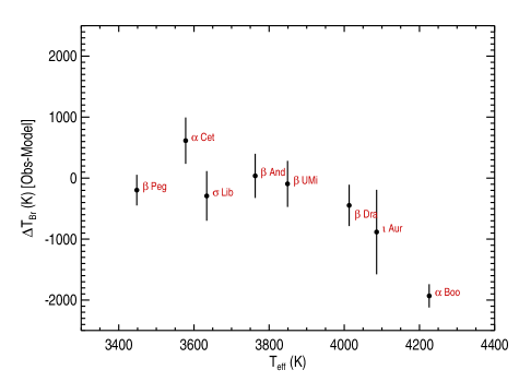
Figure 4: Dehaes et al. (2011) 1.2 mm MAMBO II: Observations minus model brightness temperatures plotted with same y-axis as used in Figure 3. The SIMBA fluxes for $\alpha$ Boo and $\alpha$ Cet lie outside this range. The model is consistent with these higher S/N fluxes, but note Dehaes et al. discount the MAMBO II fluxes for $\alpha$ Boo and $\alpha$ Cet owing to unsuitable weather conditions.

5 Comparison with Observations and Predictions

To test our semi-analytic model for the mm thermal fluxes, we require a sample of single inactive mundane red giants with well determined stellar parameters. The 250 GHz (1.2 mm) single 30 m dish IRAM survey of Altenhoff et al. (1994) presents the largest sample of measurements for these stars. We combined this survey with the accurate $\phi_{\ast}$ and $T_{\rm eff}$ sample from the Mark III optical interferometer (Mozurkewich et al., 2003). The stars in common are listed in Table 2. We also have added $\sigma$ Lib (M3 III) from the smaller sample of Dehaes et al. (2011). This combination of data enables us to make initial tests of the model. In Figure 2, we compare the observed $\langle T_{\rm Br}\rangle$ (G=1.08), with the predicted basal-limit for 250 GHz.

The spectral-types of interest are single G, K and M giants. Unfortunately there were no single G giant detections reported in the two stellar samples, so we do not consider these objects further here. Because we are interested in the chromospheric emission, we need to avoid stars with significant ionized wind opacity, as is likely to occur at lower gravity (higher luminosity), e.g., the eclipsing binary $\zeta$ Aur (K4 Ib + B5 V) (Harper et al., 2005) and its spectral-type proxy $\lambda$ Vel (K4 Ib) (Carpenter et al., 1999), and earlier spectral types. We also exclude the hybrid chromosphere stars $\gamma$ Aql (K3 II) and $\iota$ Aur (K3 II) because the hybrid $\alpha$ TrA (K3 II) shows evidence for a warm ionized wind (Harper et al., 2005). We include $\alpha$ Boo (K2 III) even though it is thought to have a 10,000 K partially ionized wind, because the mass-loss rate $\dot{M}=2\times 10^{-10}\>{\rm M}_{\odot}{\rm yr}^{-1}$ (Drake, 1985) is small, although perhaps not entirely negligible. For the later spectral-type semi-regular M giants it is not clear when the energy and momentum deposited by small amplitude radial pulsations begins dominate the sources present in earlier spectral-type red giants and begin to fundamentally alter the chromospheric structure, see for example Eaton et al. (1990). We thus include R Lyr (M5 III), while noting that Luttermoser, Johnson, & Eaton (1994) found it was not possible to construct a time-independent semi-empirical model for g Her (M6 III).

For the sample, we have estimates and errors for $\phi$, $T_{\rm eff}$ and $\hat{F}$. In Figure 3 we directly compare the model (with $G=1.08$) to Altenhoff et al. (1994). The model is broadly consistent with the observed fluxes but because of the large uncertainties ($\geq 15$%) of the IRAM measurements it is not clear whether there is additional intrinsic scatter that is not accounted for in the model. Combined Array for Research in Millimeter-wave Astronomy (CARMA) and ALMA observations with flux signal-to-noise ratios of $\sim 20$ will be a defining test of our simple model of time-independent but inhomogeneous red giant chromospheres.

5.1 Spectral Indices

Spectral indices, $\alpha$ (where $F_{\nu}\propto\nu^{\alpha}$), are an empirical measure to help interpret multi-frequency radio observation. For a constant temperature source with an angular diameter independent of frequency $\alpha=2$, reflecting the frequency factor in the Planck function. Many $\alpha$’s have been obtained at quite different frequencies where the flux can arise from different atmospheric layers (e.g., at cm-wavelengths these can reflect, say, the wind acceleration at 6 cm but the chromosphere at 2 cm), which limits their utility. With the greater sensitivity of the Karl G. Jansky Very Large Array (JVLA) and ALMA, a finer sweep of frequencies can be made and the resulting spectral energy distributions should provide more powerful diagnostic information.

Using the model above we see that the 100 GHz flux is predicted to come from the upper portion of the chromosphere: by 250 GHz the chromosphere is becoming transparent; while at 900 GHz the chromosphere can be become quite transparent, revealing the cold molecular layers above the photosphere, as seen in the CO fundamental bands (Wiedemann et al., 1994). For the sample in Table 2, we find spectral indices using ALMA Band 3 (100 GHz) and Band 9 (660 GHz) lie in the range $\sim 1.60\pm 0.15$ indicating that the mean temperatures are declining with increasing frequency.

5.2 Variability

The mm optical depths scale with chromospheric heating, so that observed changes in major cooling channel fluxes in the uv can reasonably be expected to induce corresponding changes in $\Delta\tau$, i.e., $\delta{\cal F}\propto f\left(\delta\Delta\tau\right)$. Few quantitative studies exist of the temporal chromospheric flux variability of red giants, although both $\alpha$ Boo and $\alpha$ Tau have been well observed with IUE. For $\alpha$ Tau, Cuntz et al. (1996) find a peak to peak Mg II h & k flux variations of $\pm 4$% on day time scales, whereas Robinson, Carpenter, & Brown (1998) find a slightly larger $\sim 15$% from three HST observations over seven years. McClintock et al. (1978) found little evidence for variability in $\alpha$ Boo’s chromospheric emissions above Copernicus’s instrumental noise: 25% over tens of hours and 20% on year time scales. Ayres et al. (1995) reported a 6% rms variation in the Mg II h line observed by IUE over nearly a decade, although a smaller variability on day time scales was potentially masked by a long-term $\sim 10$% secular trend. Brown et al. (2008) find long term Ca II H & K variations at the 10% level with a suggestion of a $>14$ year cycle. $\alpha$ Boo has a significant Mg II h & k emission above the basal-flux and it is possible that the excess magnetic heating is responsible for changes in the chromosphere and mm-radio emission (see also discussion in Sennhauser & Berdyugina 2011). Judge et al. (1993) have examined the chromospheric flux variations of M giants, $\rho$ Per (M4 II, $\pm 10$%), R Lyr (M5 III, $\pm 4$%), and g Her (M6 III, $\pm 10$%). These changes do not follow the variations in V magnitude. Perturbing the $\Delta\tau$’s in the analytic model by $\pm 15$% imposes a fractional change in $\langle T_{\rm Br}\rangle$ (or 250 GHz flux) of $<5$%.

On the basis of these studies we do not expect significant changes in the mm and sub-mm radio fluxes if the chromospheric material is uniformly distributed, such as may result from a high filling factor of the warm chromosphere, and/or spatial-averaged acoustic heating.

5.3 Comparison with Recent Observations

Red giants are feeble thermal radio emitters and obtaining accurate and precise fluxes is difficult. Some more recent observations have been made of red giants by Cohen et al. (2005) (interferometric) and Dehaes et al. (2011) (single dish bolometer arrays). Cohen et al. (2005) have reported BIMA mm-fluxes for $\alpha$ Tau and $\alpha$ Boo obtained at 217.8 GHz (1.38 mm) and 108.4 GHz (2.77 mm), and compared againt predictions based on photospheric Radiative Equilibrium (RE) values. Cohen et al. (2005) reported evidence for excess mm-emission from $\alpha$ Boo, which is consistent with the observed presence chromospheric heating. Further, the BIMA fluxes imply little change in temperature with frequency, whereas the present model reflects the decline of temperature as the higher frequencies probe closer to the photosphere. The 217.8 GHz flux for $\alpha$ Tau (when scaled) remains significantly lower than the IRAM 250 GHz flux. A comparison of the BIMA, RE and present model is given in Table 3.

Table 3: Observed and predicted mm fluxes (mJy) for $\alpha$ Tau and $\alpha$ Boo. Observed values are from Cohen et al. (2005) and their predictions are based on radiative equilbrium models.

	$\alpha$ Boo (K2 III)	$\alpha$ Tau (K5 III)
	217.8 GHz
Observed	$83.50\pm 17.1$	$25.78\pm 5.64$
Cohen predicted	33.43	32.38
Present Model	$\geq 52.8$	40.8
	108.4 GHz
Observed	$20.09\pm 0.69$	$13.97\pm 1.46$
Cohen Predicted	7.94	7.80
Present Model	$\geq 17.7$	15.9

Table 4: Observed and predicted 1.2 mm fluxes (mJy) for the standard stars of Dehaes et al. (2011). Note that fluxes given within ‘[]’ were discounted because of weather conditions.

	MAMBO II	SIMBA	IRAM	Predicted
Star	Dehaes et al.		Altenhoff et al.
$\alpha$ Boo (K2 III)	[$20.8\pm 3.5$]	$105.6\pm 6.9$	$78\pm 8$	$\geq 57$
$\beta$ And (M0 III)	$23.5\pm 2.7$	$<40.1$	$25\pm 4$	23
$\alpha$ Cet (M2 III)	[$23.6\pm 2.5$]	$58.3\pm 4.1$	$15\pm 3$	19
$\beta$ Peg (M2.5 III)	$29.5\pm 3.2$	$29.2\pm 2.5$	$23\pm 5$	32
$\iota$ Aur (K3 II)	$5.5\pm 1.6$	-	$13\pm 3$	$\geq 8$
$\beta$ Umi (K4 III)	$12.2\pm 1.6$	-	$16\pm 4$	13
$\gamma$ Dra (K5 III)	$10.1\pm 1.3$	-	$<12$	12
$\sigma$ Lib (M3 III)	$12.1\pm 2.0$	-	-	14

Dehaes et al. (2011) present 1.2 mm SIMBA and MAMBO II observations for a sample of red giants. We compare these measurements to the model in Table 4. In general the agreement is quite good, except for $\alpha$ Cet (M2 III). The SIMBA flux of $58.3\pm 4.1$ mJy is much greater than their MAMBO II value of $23.6\pm 2.5$ mJy, which the authors discount owing to unstable weather conditions. The later, nevertheless, is much closer to the IRAM and model fluxes. The SIMBA flux for $\alpha$ Boo is close to the Cohen et al. (2005) value (when adjusted for the different frequencies), whereas our prediction is closer to IRAM. These measurements were made at different epochs, however.

The limited data hint at variability at mm-wavelengths that is larger than one might anticipate based on the small observed chromospheric variability (peak-to-peak 15% that implies 4% in mm fluxes)

6 Discussion

The time-independent inhomogeneous model appears to be consistent with most existing mm-radio observations. However, because most measurements were made at a single frequency and have sizeable flux uncertainties, these data are only just beginning to provide insight into the chromospheres of inactive K and M giants. The characteristic temperatures of stellar chromospheres: $T^{\rm uv}_{\rm Min}$, $T_{\rm CO}$, $T_{\rm Int}$, and $T_{\rm Chrom}$ all are within 50% of the mean, and the unfortunate reality is that there is limited thermal dynamic range in this problem. The errors on $\phi_{\ast}$ and $T_{\rm eff}$ are at the few percent level so to test the limits of this model will require multi-frequency observations with S/N $\sim 20$ and as good an absolute calibration as possible ($\sim 5$%), both of which are challenging. Multiple observations at closely spaced frequencies are highly desirable, because each flux would have a contribution from overlapping spatial regions and provide a much better measure of the mean temperature gradient than spectral indices based on widely separated frequencies. On this point we note that using $T_{\rm eff}$ and $\phi_{\ast}$ to estimate the mm-radio flux in equation (4) can give reasonable values even though it is a physically unsound model.

We have not explored the G giants, but the model could be extended to include a filling factor of hotter material not at the boundary layer temperature (Wiedemann et al., 1994) by setting, for example, $T_{\rm CO}=T^{\rm uv}_{\rm Min}$ for that component.

6.1 Variability

Millimetre observations, such as those from JVLA Q-band, CARMA, and ALMA, have the potential to distinguish between the debated acoustic or magnetic origin of chromospheric basal-flux heating. Numerical simulations show that granule sizes for main-sequence and giant stars scale with the surface pressure scale-height (Freytag et al., 2002; Nordlund & Dravins, 1990) and the grain size is $\sim 10H_{\rm pres}$. The number of granules on the stellar surface will scale as

$$N_{\rm gran}\simeq 4\times 10^{6}\left({R_{\odot}\over{R_{\star}}}\right)^{2}\left({T_{{\rm eff},\odot}\over{T_{{\rm eff},\star}}}\right)^{2}\left({M_{\star}\over{M_{\odot}}}\right)^{2}$$ (22)

which for $\alpha$ Tau gives $\sim 10,000$ granules on the visible disk. This scaling appears consistent with findings from Kepler (Mathur et al., 2011). If the horizontal coherence scale of the acoustic shock heating is of the order of the granule size (Loukitcheva et al., 2008) then the spatially unresolved radio flux will have contributions from $\sim 10,000$ phase-uncorrelated patches. In the acoustic shocked heated interpretation, at any one moment there are likely to be several shocks passing through each patch, so one might expect that a basal-flux red giant to show quite small variability at mm wavelengths in this scenario. Barring limb projection effects, the rms fractional fluctuations of the total intensity would be of order $1/\sqrt{10,000}=0.01$. However, if observations show significant variability, then it is likely that there is an additional, spatially more correlated source of chromospheric heating, i.e., magnetic active regions or possibly non-radial pulsations. To explore this aspect, it would be important to observe giant stars whose Mg II h & k or Ca II H & K fluxes are as close to the basal limit as possible.

6.2 Molecular Component

In the Sun the temperature minimum appears to be set by the balance between mechanical heating and cooling by H^-. Above this temperature minimum there appears to be an unknown fraction, perhaps as much as 80%, of the surface covered by CO clouds or columns (Ayres, 2002). In the red giants the CO, which appears to be close to radiative equilibrium temperatures, appears to cover most of the stellar surfaces. g Her (30 Her, M6 III, $\phi=19$ mas, $T_{\rm eff}=3010$ K) was not detected in the Altenhoff et al. (1994) survey ($<6$ mJy) and the upper-limit to its brightness temperature is only 465 K. The present model predicts 28 mJy and this is very discrepant. The star has been observed with both IUE (Judge et al., 1993) and HST (Luttermoser et al., 1994) and it shows uv chromospheric emission. g Her and R Lyr both have similar $\phi_{\ast}$ and $T_{\rm eff}$ and have similar 2 cm radio VLA fluxes (Drake et al., 1991). In the model presented here we adopted $T_{\rm CO}=0.6T_{\rm eff}$, but if the low fluxes for g Her and R Lyr are confirmed then the molecular component of the outer atmosphere may be even cooler, perhaps dominated by an H₂O molsphere; and M5 III may mark the onset of a cooler dominant component. However, even this would not seem enough to explain g Her’s low 1.2 mm flux and multi-frequency observations are urgently needed. $\gamma$ Cru (M3 III) has been observed with the ATCA at 94 GHz . It has a large angular diameter ($\phi_{\ast}\simeq 25$ mas, $T_{\rm eff}=3626$ K; Ireland et al. 2004; Cohen et al. 1996) and the present model predicts $\sim 16$ mJy but the observed flux is significantly less (M. Cohen, priv comm.).

It would seem that K and early M giants at the basal-limit might be suitable mm flux calibrators at the 5% level. Random fluctuations in the brightness resulting from changes at the stellar photospheric granule scale should average down, and chromospheric heating fluctuations derived from optical and uv emission suggest small variations in the mm-fluxes. For later spectral-types, the uncertain influence of this variable chromospheric heating is further reduced. That being said, the emission from the molecular material mixed in with warmer chromospheric plasma needs to be calibrated in some way, because it is challenging to establish directly from theoretical models or simulations of stellar atmospheres.

The semi-analytic model developed here is a time-independent 1-D model with all the inherent assumptions. When the next generation of theoretical chromospheric heating models becomes available, one could analyse the thermodynamic structure and develop a new analytic representation. Until then, the present model, based on the interpretation of empirical evidence should be regarded as a starting point. Even if real red giant chromospheres are highly time variable, the semi-empirical models upon which our mm radio predictor is based, still represent a measure of the temperatures, electron densities, and ionization required to produce the uv and optical spectral diagnostics. One could imagine an actual atmosphere as being a highly dynamic jumbled-up 1-D model, in which case the temperature rise in the warm chromosphere no longer is monotonic. The implication for the radio fluxes would be to reduce them slightly as cool material is now present at greater altitudes. This systematic bias is being investigated.

A test of chromospheric models for the largest angular diameter giants may be possible with ALMA, at frequencies above 250 GHz, in its most extended (16  km maximum baseline) configuration. The chromospheres will be partially resolved but they will provide constraints on the millimetre limb brightening or darkening.

7 Conclusions

We present a semi-analytic ’toy’ chromospheric model to examine millimetre thermal continuum radio fluxes of non-dusty and non-pulsating red giants. Equation (15) shows, in a clear fashion, the contributions to the brightness temperature from the cool molecular layers at the base, and from the chromosphere itself, through weighting factors obtained from analytic solutions to the radiative transfer equation. At 3 mm, the chromospheres are semi-opaque; while at 1.2 mm the chromosphere becomes optically thin and the cool molecular material becomes visible. The model predicts a basal level of radio emission that depends on the temperature of the boundary layers. Studies at (sub-) mm will provide new insights into these especially enigmatic molecular regions. The model also permits an analysis of radio flux variability in response to changes in chromospheric heating as observed in Mg II h & k or Ca II H & K. If the chromospheric heating rate is not known for a given red giant, the model still can predict the basal mm radio fluxes. Significant variations in radio emission for basal-flux red giants, if detected, would indicate a source of structured large-scale heating, possibly magnetic in nature. The physical arrangement, e.g., columns and sheets, of the cool and warm chromospheric plasma can be constrained by the mm-radio limb-brightening of red giants that can be spatially resolved when ALMA reaches its maximum baselines. A good test of this semi-analytic model would be to compare it against red giants with independently determined $T_{\rm eff}$, $\phi_{\ast}$, and $T_{\rm CO}$ and that can be monitored for changes in chromospheric heating.

In summary, the present analytic model is consistent with most existing radio measurements and also highlights some possible anomalies. The sensitivity of mm-fluxes to changes in chromospheric heating can be evaluated and spectral indices are predicted for the existing thermal gradients. When a sample of multiwavelength (sub-) mm-radio observations with good signal-to-noise becomes available these can be used to test the overall validity of the model. If the model passes this test, i.e., if there are not significant star to star discrepancies, the observations can then be used to refine and test the mean thermal gradient in the stellar chromospheres. The spectral shapes could be used to better describe the outward temperature gradient, or alternately they could invalidate the present model completely if there is no outward temperature increase. More importantly, these important new radio observations can test new 3-D theoretical heating models when they become available.

There appear to be a few stars with significant 1.2 mm flux differences between widely separated epochs and different observing facilities that appear at first sight to be larger than one would expect based on observed changes in chromospheric heating. These would suggest significant magnetic contributions for stars at twice the basal uv-flux levels. We also have identified a few of late M giants which, while at the limit of applicability of the model, seem to have very low observed fluxes. However, we must await accurate new observations of these stars before we can draw any significant conclusions.

While optical angular diameters and effective temperatures for many giants are known to a precision and accuracy of a few percent, we have shown that the physical dynamic range of $T_{\rm Br}$ for the mm-radio problem is limited. Future progress will require high S/N multi-wavelength (sub-) mm radio fluxes with as small absolute flux calibration errors as possible.

References

- Altenhoff et al. (1960) Altenhoff W. J., Mezger P. G., Wendker H. J., Westerhout G., 1960, Veröff. Sternwärte, Bonn, 59, 48
- Altenhoff et al. (1994) Altenhoff W. J., Thum C., Wendker H. J., 1994, A&A, 281, 161
- Ayres (1979) Ayres T. R., 1979, ApJ, 228, 509
- Ayres (2002) —, 2002, ApJ, 575, 1104
- Ayres et al. (1995) Ayres T. R., Fleming T. A., Simon T., Haisch B. M., Brown A., Lenz D., Wamsteker W., de Martino D., Gonzalez C., Bonnell J., Mas-Hesse J. M., Rosso C., Schmitt J. H. M. M., Truemper J., Voges W., Pye J., Dempsey R. C., Linsky J. L., Guinan E. F., Harper G. M., Jordan C., Montesinos B. M., Pagano I., Rodono M., 1995, ApJS, 96, 223
- Ayres & Linsky (1975) Ayres T. R., Linsky J. L., 1975, ApJ, 200, 660
- Ayres et al. (1974) Ayres T. R., Linsky J. L., Shine R. A., 1974, ApJ, 192, 93
- Ayres & Testerman (1981) Ayres T. R., Testerman L., 1981, ApJ, 245, 1124
- Baines et al. (2010) Baines E. K., Döllinger M. P., Cusano F., Guenther E. W., Hatzes A. P., McAlister H. A., ten Brummelaar T. A., Turner N. H., Sturmann J., Sturmann L., Goldfinger P. J., Farrington C. D., Ridgway S. T., 2010, ApJ, 710, 1365
- Berio et al. (2011) Berio P., Merle T., Thévenin F., Bonneau D., Mourard D., Chesneau O., Delaa O., Ligi R., Nardetto N., Perraut K., Pichon B., Stee P., Tallon-Bosc I., Clausse J. M., Spang A., McAlister H., Ten Brummelaar T., Sturmann J., Sturmann L., Turner N., Farrington C., Goldfinger P. J., 2011, A&A, 535, A59
- Brown et al. (2008) Brown K. I. T., Gray D. F., Baliunas S. L., 2008, ApJ, 679, 1531
- Buchholz et al. (1998) Buchholz B., Ulmschneider P., Cuntz M., 1998, ApJ, 494, 700
- Butler & Wooten (1999) Butler B., Wooten A., 1999, ALMA Memo., 276, 1
- Byrne et al. (1988) Byrne P. B., Murphy H. M., Dufton P. L., Kingston A. E., Lennon D. J., 1988, A&A, 197, 205
- Carlsson & Stein (1995) Carlsson M., Stein R. F., 1995, ApJ, 440, L29
- Carpenter et al. (1999) Carpenter K. G., Robinson R. D., Harper G. M., Bennett P. D., Brown A., Mullan D. J., 1999, ApJ, 521, 382
- Cohen et al. (2005) Cohen M., Carbon D. F., Welch W. J., Lim T., Schulz B., McMurry A. D., Forster J. R., Goorvitch D., 2005, AJ, 129, 2836
- Cohen et al. (1996) Cohen M., Witteborn F. C., Carbon D. F., Davies J. K., Wooden D. H., Bregman J. D., 1996, AJ, 112, 2274
- Cuntz et al. (1996) Cuntz M., Deeney B. D., Brown A., Stencel R. E., 1996, ApJ, 464, 426
- Decin et al. (2003) Decin L., Vandenbussche B., Waelkens C., Decin G., Eriksson K., Gustafsson B., Plez B., Sauval A. J., 2003, A&A, 400, 709
- Dehaes et al. (2011) Dehaes S., Bauwens E., Decin L., Eriksson K., Raskin G., Butler B., Dowell C. D., Ali B., Blommaert J. A. D. L., 2011, A&A
- Drake (1985) Drake S. A., 1985, in NATO ASIC Proc. 152: Progress in Stellar Spectral Line Formation Theory, J. E. Beckman & L. Crivellari, ed., pp. 351–357
- Drake et al. (1991) Drake S. A., Linsky J. L., Judge P. G., Elitzur M., 1991, AJ, 101, 230
- Eaton (1993) Eaton J. A., 1993, ApJ, 404, 305
- Eaton et al. (1990) Eaton J. A., Johnson H. R., Cadmus Jr. R. R., 1990, ApJ, 364, 259
- Eriksson et al. (1983) Eriksson K., Linsky J. L., Simon T., 1983, ApJ, 272, 665
- Fontenla et al. (1990) Fontenla J. M., Avrett E. H., Loeser R., 1990, ApJ, 355, 700
- Fontenla et al. (2009) Fontenla J. M., Curdt W., Haberreiter M., Harder J., Tian H., 2009, ApJ, 707, 482
- Freytag et al. (2002) Freytag B., Steffen M., Dorch B., 2002, Astronomische Nachrichten, 323, 213
- Harper (1992) Harper G. M., 1992, MNRAS, 256, 37
- Harper et al. (2005) Harper G. M., Brown A., Bennett P. D., Baade R., Walder R., Hummel C. A., 2005, AJ, 129, 1018
- Harper et al. (2001) Harper G. M., Brown A., Lim J., 2001, ApJ, 551, 1073
- Hummer (1988) Hummer D. G., 1988, ApJ, 327, 477
- Ireland et al. (2004) Ireland M. J., Tuthill P. G., Bedding T. R., Robertson J. G., Jacob A. P., 2004, MNRAS, 350, 365
- Judge & Carpenter (1998) Judge P. G., Carpenter K. G., 1998, ApJ, 494, 828
- Judge et al. (1993) Judge P. G., Luttermoser D. G., Neff D. H., Cuntz M., Stencel R. E., 1993, AJ, 105, 1973
- Judge & Stencel (1991) Judge P. G., Stencel R. E., 1991, ApJ, 371, 357
- Kalkofen et al. (1999) Kalkofen W., Ulmschneider P., Avrett E. H., 1999, ApJ, 521, L141
- Kelch et al. (1978) Kelch W. L., Chang S.-H., Furenlid I., Linsky J. L., Basri G. S., Chiu H.-Y., Maran S. P., 1978, ApJ, 220, 962
- Leenaarts et al. (2011) Leenaarts J., Carlsson M., Hansteen V., Gudiksen B. V., 2011, A&A, 530, A124
- Linsky & Avrett (1970) Linsky J. L., Avrett E. H., 1970, PASP, 82, 169
- Linsky & Ayres (1978) Linsky J. L., Ayres T. R., 1978, ApJ, 220, 619
- Loukitcheva et al. (2004) Loukitcheva M., Solanki S. K., Carlsson M., Stein R. F., 2004, A&A, 419, 747
- Loukitcheva et al. (2008) Loukitcheva M. A., Solanki S. K., White S., 2008, Astrophys Space Sci, 313, 197
- Luttermoser et al. (1994) Luttermoser D. G., Johnson H. R., Eaton J., 1994, ApJ, 422, 351
- Martínez et al. (2011) Martínez M. I. P., Schröder K.-P., Cuntz M., 2011, MNRAS, 348
- Mathur et al. (2011) Mathur S., Hekker S., Trampedach R., Ballot J., Kallinger T., Buzasi D., García R. A., Huber D., Jiménez A., Mosser B., Bedding T. R., Elsworth Y., Régulo C., Stello D., Chaplin W. J., De Ridder J., Hale S. J., Kinemuchi K., Kjeldsen H., Mullally F., Thompson S. E., 2011, ApJ, 741, 119
- McClintock et al. (1978) McClintock W., Moos H. W., Henry R. C., Linsky J. L., Barker E. S., 1978, ApJS, 37, 223
- McMurry (1999) McMurry A. D., 1999, MNRAS, 302, 37
- Mozurkewich et al. (2003) Mozurkewich D., Armstrong J. T., Hindsley R. B., Quirrenbach A., Hummel C. A., Hutter D. J., Johnston K. J., Hajian A. R., Elias II N. M., Buscher D. F., Simon R. S., 2003, AJ, 126, 2502
- Nordlund & Dravins (1990) Nordlund A., Dravins D., 1990, A&A, 228, 155
- Ohnaka et al. (2012) Ohnaka K., Hofmann K.-H., Schertl D., Weigelt G., Malbet F., Massi F., Meilland A., Stee P., 2012, A&A, 537, A53
- Olson & Kunasz (1987) Olson G. L., Kunasz P. B., 1987, JQSRT, 38, 325
- Perrin et al. (2004) Perrin G., Ridgway S. T., Mennesson B., Cotton W. D., Woillez J., Verhoelst T., Schuller P., Coudé du Foresto V., Traub W. A., Millan-Gabet R., Lacasse M. G., 2004, A&A, 426, 279
- Quirrenbach et al. (1993) Quirrenbach A., Mozurkewich D., Armstrong J. T., Buscher D. F., Hummel C. A., 1993, ApJ, 406, 215
- Robinson et al. (1998) Robinson R. D., Carpenter K. G., Brown A., 1998, ApJ, 503, 396
- Rowe (1992) Rowe A. K., 1992, in Astronomical Society of the Pacific Conference Series, Vol. 26, Cool Stars, Stellar Systems, and the Sun, Giampapa M. S., Bookbinder J. A., eds., p. 561
- Rybicki & Lightman (2004) Rybicki G. B., Lightman A. P., 2004, Radiative Processes in Astrophysics, Wiley-VCH Verlag GmbH & Co. KGaA
- Schrijver & Zwaan (2000) Schrijver C. J., Zwaan C., 2000, Solar and Stellar Magnetic Activity, Cambridge Astrophysics Series 34, Cambridge University Press
- Sennhauser & Berdyugina (2011) Sennhauser C., Berdyugina S. V., 2011, A&A, 529, A100
- Tsuji (2008) Tsuji T., 2008, A&A, 489, 1271
- Tsuji et al. (1997) Tsuji T., Ohnaka K., Aoki W., Yamamura I., 1997, A&A, 320, L1
- Uitenbroek (1989) Uitenbroek H., 1989, A&A, 213, 360
- Ulmschneider (1991) Ulmschneider P., 1991, in Mechanisms of Chromospheric and Coronal Heating, P. Ulmschneider, E. R. Priest, & R. Rosner, ed., pp. 328–+
- Vecchio et al. (2009) Vecchio A., Cauzzi G., Reardon K. P., 2009, A&A, 494, 269
- Vernazza et al. (1976) Vernazza J. E., Avrett E. H., Loeser R., 1976, ApJS, 30, 1
- Vernazza et al. (1981) —, 1981, ApJS, 45, 635
- Wedemeyer-Böhm et al. (2007) Wedemeyer-Böhm S., Ludwig H. G., Steffen M., Leenaarts J., Freytag B., 2007, A&A, 471, 977
- Wiedemann et al. (1994) Wiedemann G., Ayres T. R., Jennings D. E., Saar S. H., 1994, ApJ, 423, 806