Atmospheric extinction properties above Mauna Kea from the Nearby Supernova Factory spectro-photometric data set

We present a new atmospheric extinction curve for Mauna Kea spanning 3200–9700 Å. It is the most comprehensive to date, being based on some 4285 standard star spectra obtained on 478 nights spread over a period of 7 years obtained by the Nearby SuperNova Factory using the SuperNova Integral Field Spectrograph. This mean curve and its dispersion can be used as an aid in calibrating spectroscopic or imaging data from Mauna Kea, and in estimating the calibration uncertainty associated with the use of a mean extinction curve. Our method for decomposing the extinction curve into physical components, and the ability to determine the chromatic portion of the extinction even on cloudy nights, is described and verified over the wide range of conditions sampled by our large dataset. We demonstrate good agreement with atmospheric science data obtain at nearby Mauna Loa Observatory, and with previously published measurements of the extinction above Mauna Kea.

1 Introduction

The summit of Mauna Kea in Hawaii is home to the largest and most powerful collection of astronomical telescopes in the world. For many studies accurate flux calibration is critical for deriving the maximum amount of information from observations with these telescopes, and correction for the optical atmospheric and instrumental transmissions is one of the main limitations of astronomical flux measurements from the ground (see Burke et al., 2010; Patat et al., 2011, for the most recent reviews). Therefore, as part of our Nearby SuperNova Factory project (SNfactory, Aldering et al., 2002) we have carefully monitored the atmospheric transmission over the course of our observing campaign, and in this paper describe findings that should be of use to other Mauna Kea observers.

According to the GONG (Global Oscillation Network Group) site survey (Hill et al., 1994b, a), the extinction above the summit of Mauna Kea is among the lowest and most stable of any astronomical site. Several studies were carried out at the end of the 80’s to assess the atmospheric characteristics above Mauna Kea (Krisciunas et al., 1987; Boulade, 1987; Bèland et al., 1988). These have formed the basis for the standard Mauna Kea extinction curve provided by most observatories on Mauna Kea. However, the results reported by Boulade (1987) and Bèland et al. (1988) are single-night extinction studies carried out using the 3.6 m Canada France Hawaii Telescope (CFHT) over limited wavelength ranges (3100–3900 Å and 3650–5850 Å, respectively). Thus, they do not cover the entire optical window, nor do they reflect variability of the extinction. The measurements of the optical extinction from the Mauna Kea summit presented in Krisciunas et al. (1987) are based on 27 nights of $B$ and $V$ band ($\sim 4400$ Å and $\sim 5500$ Å) measurements from three different telescopes, including the 2.2 m University of Hawaii telescope (UH88) and the CFHT, between 1983 and 1985. Since then, only the evaluation of the quality of the site for the Thirty Meter Telescope (TMT) has been published (Schöck et al., 2009; Travouillon et al., 2011). The TMT site testing campaign confirms that Mauna Kea is one of the best sites for ground based astronomy but does not include the properties and the variability of the spectral extinction at the site.

SNfactory (Aldering et al., 2002) was developed for the study of dark energy using Type Ia supernovae (SNe Ia). Our goal has been to find and study a large sample of nearby SNe Ia, and to achieve the percent-level spectro-photometric calibration necessary so that these SNe Ia can be compared with SNe Ia at high redshifts. Since 2004 the SNfactory has obtained spectral time series of over 200 thermonuclear supernovæ and these are being used to measure the cosmological parameters and improve SNe Ia standardization by empirical means and through a better understanding of the underlying physics. The main asset of the SNfactory collaboration is the SuperNova Integral Field Spectrograph (SNIFS, Lantz et al., 2004), a dedicated integral field spectrograph built by the collaboration and mounted on the University of Hawaii UH88 telescope.

Along with the supernova observations, the SNfactory data set includes spectro-photometric observations of standard stars with SNIFS, which are used to obtain the instrumental calibration and the atmospheric extinction. The observations benefit from a large wavelength range (3200–9700 Å) and the high relative precision that SNIFS can achieve. When possible, standards were obtained throughout a given night to help distinguish between spectral and temporal variations of the transmission. While it is common practice to derive an extinction curve by solving independently for the extinction at each wavelength, this approach ignores the known physical properties of the atmosphere, which are correlated across wide wavelength regions. Using the standard star spectra to disentangle the physical components of the atmosphere extinction ensures a physically meaningful result, allows for robust interpolation across standard star spectral features, and provides a simpler and more robust means of estimating the error covariance matrix. The method described in this paper allows us to obtain such a complete atmospheric model for each observation night, including nights afflicted by clouds. We use the results to generate a new mean Mauna Kea extinction curve, and to explore issues related to variation in the extinction above Mauna Kea.

2 The SNfactory Mauna Kea extinction dataset

We begin by describing the basic properties of the dataset to be used in measuring the extinction properties above Mauna Kea.

2.1 The Supernova Integral Field Spectrograph & data reduction

SNIFS is a fully integrated instrument optimized for automated observation of point sources on a structured background over the full optical window at moderate spectral resolution. It consists of a high-throughput wide-band pure-lenslet integral field spectrograph (IFS, “à la TIGER”; Bacon et al., 1995, 2001), a multifilter photometric channel to image the field surrounding the IFS for atmospheric transmission monitoring simultaneous with spectroscopy, and an acquisition/guiding channel. The IFS possesses a fully filled $6\aas@@fstack{\prime\prime}4\times 6\aas@@fstack{\prime\prime}4$ spectroscopic field of view subdivided into a grid of $15\times 15$ spatial elements (spaxels), a dual-channel spectrograph covering 3200–5200 Å and 5100–9700 Å simultaneously, and an internal calibration unit (continuum and arc lamps). SNIFS is continuously mounted on the south bent Cassegrain port of the University of Hawaii 2.2 m telescope on Mauna Kea, and is operated remotely. The SNIFS standard star spectra were reduced using our dedicated data reduction procedure, similar to that presented in Section 4 of Bacon et al. (2001). A brief discussion of the spectrographic pipeline was presented in Aldering et al. (2006). Here we outline changes to the pipeline since that work, but leave a complete discussion of the reduction pipeline to subsequent publications focused on the instrument itself.

After standard CCD preprocessing and subtraction of a low-amplitude scattered-light component, the 225 spectra from the individual spaxels of each SNIFS exposure are extracted from each blue and red spectrograph exposure, and re-packed into two $(x,y,\lambda)$-datacubes. This highly specific extraction is based upon a detailed optical model of the instrument including interspectrum crosstalk corrections. The datacubes are then wavelength-calibrated using arc lamp exposures acquired immediately after the science exposures, and spectro-spatially flat-fielded using continuum lamp exposures obtained during the same night. Cosmic rays are detected and corrected using a three-dimensional-filtering scheme applied to the datacubes.

Standard star spectra are extracted from each $(x,y,\lambda)$-datacube using a chromatic spatial point-spread function (PSF) fit over a uniform background (Buton, 2009). The PSF is modeled semi-analytically as a constrained sum of a Gaussian (describing the core) and a Moffat function (simulating the wings). The correlations between the different shape parameters, as well as their wavelength dependence, were trained on a set of 300 standard star observations in various conditions of seeing and telescope focus between 2004 and 2007 with SNIFS. This resulted in a empirical chromatic model of the PSF, depending only on an effective width (accounting for seeing) and a flattening parameter (accounting for small imaging defocus and guiding errors). The PSF modeling properly takes the wavelength-dependent position shift induced by atmospheric differential refraction into account without resampling.

2.2 Data characteristics and sub-sample selection

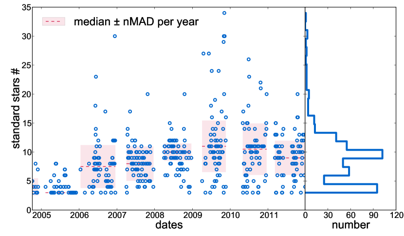
(a) Number of standard stars per night

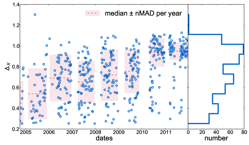
(b) Airmass range ($\Delta_{X}$) per night

Figure 1: Time evolution of the standard star number (# standards) per night LABEL:sub@fig:standards-number and of the airmass range ($\Delta_{X}$) per night LABEL:sub@fig:standards-airmass after quality cuts. The nMAD acronym stands for “normalized median absolute deviation” (the normalization factor is introduced in order to use the median absolute deviation as a consistent estimator for the estimation of the standard deviation).

The SNfactory spectro-photometric follow-up has been running regularly since September 2004, with a periodicity of two to three nights. In most years observations were concentrated in the April to December period in order to coincide with the best weather at Palomar where we carried out our search for supernovæ. Initially the nights were split with UH observers, with SNfactory taking the second half of allocated nights. In May 2006, our program switched from half-night to full-night observations. The SNfactory time was mainly used to observe SNe Ia (up to 20 per night), but in order to flux calibrate the supernova data, standard star observations were inserted throughout the night.

Two different kinds of standard stars were observed: bright standard stars ($V=4\text{--}7$) were mainly observed during nautical twilight, while faint standard stars ($V=10\text{--}14$) were observed during astronomical twilight and during the night. A list of the standard stars used for calibration purposes by the SNfactory is given in Table 5. A typical night started with $\sim 3$ bright standard stars and one faint standard star during evening twilight, followed by 3 to 4 faint standard stars distributed all along the night in between supernovæ, and finished with another faint standard and $\sim 3$ bright standard stars during morning twilight. Generally the calibration provided in the literature for the fainter stars is of higher quality. Moreover, we found that the very short (1–2 second) exposures required for bright standard stars resulted in very complex PSF shapes. During the period when observations were conducted only during the second half of the night, the typical number of standard stars was more limited, as seen in Fig. 1a.

The evolution through the years in the number of standard stars observed per night is shown in Fig. 1a, while Fig. 1b shows the airmass range. The noticeable changes in the numbers and airmass distribution have several causes. As mentioned above, the half-night allocations up through May 2006 restricted the number of standard stars that could be observed each night without adversely impacting our SN program. In addition, in order to improve the automation in executing our observing program we developed algorithms to select a standard star during windows slated for standard star observations. Initially the selections were pre-planned manually each night, but this approach was not sufficiently flexible, e.g. to account for weather interruptions. In fall 2005 we developed an automated selection algorithm designed to pick an observable star that was best able to decorrelate airmass and spectral type based on the standard stars previously observed that night. The idea here was to obtain a good airmass range and observe enough different stellar spectral classes to avoid propagating stellar features into the calibration. More recently, having convinced ourselves that stellar features did not present a problem when using the physical extinction model presented here, the automated selection was changed so as to minimize the extinction uncertainty, considering the standard stars previously observed that night. Occasionally, nights when the Moon was full were dedicated to intensive observations of standard stars as a means of testing various aspects of our method and software implementation. Finally, a few inappropriate standard stars – Hiltner600 (double star), HZ4, LTT7987, GRW+705824 (broad-line DA white dwarfs) – have been phased out and are not included in the analysis presented here.

Of the 711 nights originally available with spectroscopic data, we removed 77 nights with only one or no standard star available. These occurred primarily due to unplanned telescope closures during the night caused by weather or technical problems. Such cases were concentrated during the period when only half-nights were available. For these nights, since an extinction solution is not possible, a mean atmospheric extinction is used for the flux calibration of the science targets. To ensure the quality of the Mauna Kea extinction determination for the present study, we also choose to discard nights with an expected extinction error larger than 0.1 magnitude/airmass; this resulted in the exclusion of an additional 55 nights. The expected extinction accuracy was calculated using the known airmass distribution of the standard stars and using the achromatic extraction error of 3% and 2% empirically found for bright and faint standard stars, respectively (Buton, 2009). Calibration of science data on such nights is not necessarily a problem, it is simply that the atmospheric properties are difficult to decouple from the instrument calibration on such nights. Finally, strict quality cuts on the number of stars ($\geq 3$) and airmass range ($\geq 0.25$) per night are applied (respectively 68 and 33 nights are skipped). Additional cuts based on flags from the pre-processing steps and the quality of the fit were applied to avoid bad exposures or spectra with production issues. In the end, the data sample is comprised of 4285 spectra from 478 nights that passed these very restrictive cuts.

3 Flux calibration formalism

In a given night the spectrum, $S_{i}(\lambda,\hat{z}_{i},t)$, of an astronomical source $i$ observed by SNIFS can be expressed as,

$$S_{i}(\lambda,\hat{z}_{i},t)=S^{\star}_{i}(\lambda,t)\times C(\lambda,t)\times T_{\mathrm{atm}}(\lambda,\hat{z}_{i},t),$$ (1)

where $S^{\star}_{i}(\lambda,t)$ is the intrinsic spectrum of the source as it would be seen from above the atmosphere, $T_{\mathrm{atm}}(\lambda,\hat{z},t)$ is the time-dependent, line-of-sight ($\hat{z}$) dependent atmospheric transmission. $C(\lambda,t)$ is the instrument calibration (i.e. the combined response of the telescope, the instrument and the detector), such that,

$$C(\lambda,t)=T_{\mathrm{tel}}(\lambda,t)\times T_{\textsc{SNIFS}}(\lambda,t)\times Q(\lambda,t)$$ (2)

where $T_{\mathrm{tel}}(\lambda,t)$, $T_{\textsc{SNIFS}}(\lambda,t)$ and $Q(\lambda,t)$ are respectively the chromatic telescope transmission, instrument transmission and detector quantum efficiency, all of which are potentially time dependent.

Because the data are divided by a flat-field exposure that is not required to be the same from night to night, we are interested only in $t$ spanning one night intervals. We will assume that the instrument response is stable over the course of a night, and therefore write:

$$C(\lambda,t)=C(\lambda).$$ (3)

Later, in § 9.2, we re-examine this question and confirm that it is valid at a level much better than 1%.

As for the atmospheric extinction, we choose to separate $T_{\mathrm{atm}}(\lambda,\hat{z}_{i},t)$ with respect to its time dependence, as follows:

$$T_{\mathrm{atm}}(\lambda,\hat{z}_{i},t)=\overline{T}_{\mathrm{atm}}(\lambda,\hat{z}_{i})\times\delta T_{i}(\lambda,\hat{z}_{i},t).$$ (4)

Here $\delta T_{i}(\lambda,\hat{z_{i}},t)$ represents the normalized atmospheric transmission variability at the time, $t$, along the line of sight, $\hat{z}_{i}$, to the star $i$. By definition, a photometric night is one in which the $\delta T_{i}$ are retrospectively found to be compatible with 1 (taking into account the measurement errors), irrespectively of wavelength, direction, or time.

Furthermore, it is common in astronomy to express the extinction in magnitudes, such that the transmission, $\overline{T}_{\mathrm{atm}}(\lambda,\hat{z})$, is given by

$$\overline{T}_{\mathrm{atm}}(\lambda,\hat{z})=10^{-0.4\times K_{\mathrm{atm}}(\lambda,\hat{z})},$$ (5)

where $K_{\mathrm{atm}}(\lambda,\hat{z})$ is the atmospheric extinction in magnitudes per airmass.

Overall, Eq. (1) becomes:

$$\log\frac{S_{i}(\lambda,\hat{z}_{i},t)}{S^{\star}_{i}(\lambda,t)}=\log C(\lambda)-0.4\times K_{\mathrm{atm}}(\lambda,\hat{z}_{i})+\log\delta T_{i}(\lambda,\hat{z}_{i},t).$$ (6)

For standard star observations, $S^{\star}(\lambda,t)$ is supposedly known (cf. § 6) and the unknowns are $C(\lambda)$, $K_{\mathrm{atm}}(\lambda,\hat{z})$ and the $\delta T_{i}(\lambda,\hat{z}_{i},t)$ (one per star $i$). Conversely, for a supernova observation, $S^{\star}(\lambda,t)$ becomes the unknown, and $C(\lambda)$, $K_{\mathrm{atm}}(\lambda,\hat{z})$ and any deviation of $\delta T_{i}(\lambda,\hat{z},t)$ from unity would need to be known in order to achieve flux calibration. As outlined in Aldering et al. (2002) and Pereira (2008), with SNIFS, $\delta T_{i}(\lambda,\hat{z},t)$ can be determined from secondary stars on the parallel imaging channel for fields having at least one visit on a photometric night.

Our focus in this paper is on the properties of the atmospheric extinction, $K_{\mathrm{atm}}(\lambda,\hat{z})$. But as we have just seen, its determination is linked to the determination of the instrument calibration, $C(\lambda)$, and of any atmospheric transmission variations with time, $\delta T_{i}(\lambda,\hat{z}_{i},t)$, for each standard star, $i$. In order to constrain the extinction, $K_{\mathrm{atm}}(\lambda,\hat{z})$, to have a meaningful shape, we now present its decomposition into physical components.

4 Atmospheric extinction model

It is now well established that the wavelength dependence of the atmospheric extinction, $K_{\mathrm{atm}}(\lambda,\hat{z})$, is the sum of physical elementary components (Hayes & Latham, 1975; Wade & Horne, 1988; Stubbs et al., 2007), either scattering or absorption. Furthermore, the extinction increases with respect to airmass $X$ along the line of sight, $\hat{z}$, giving:

$$K_{\mathrm{atm}}(\lambda,\hat{z})=\sum_{j}X^{\rho_{j}}(\hat{z})\times k_{j}(\lambda).$$ (7)

Here the different physical components $j$ are:

• Rayleigh scattering, $k_{R}$,

• aerosol scattering, $k_{A}$,

• ozone absorption, $k_{\mathrm{O_{3}}}$,

• telluric absorption, $k_{\oplus}$.

$X$ denotes airmass, and $\rho_{j}$ is an airmass correction exponent (Beer-Lambert law in presence of saturation), with $\rho_{j}=1$ (Rufener, 1986; Burke et al., 2010) for all but the telluric component.

In the following subsections, we will present the different extinction components as well as the time dependent part of the atmospheric transmission, $\delta T_{i}$.

4.1 Light scattering

The treatment of light scattering depends on the ratio between the scattering particle size and incident wavelength. Light scattering by particles of size comparable to the incident wavelength is a complicated problem which has an exact solution only for a homogeneous sphere and a given refractive index. This solution was proposed by Mie (1908) to study the properties of light scattering by aqueous suspensions of gold beads. A limiting case of this problem — the Born approximation in quantum mechanics — is Rayleigh scattering, for which the size of the particles is very small compared to the incident wavelength. At the other extreme, when the wavelength becomes much smaller than the size of the scattering particles (like the water droplets or ice crystals in the clouds), the scattering cross section becomes constant and of order of the geometrical cross section. We cover these different cases in the following subsections.

4.1.1 Rayleigh scattering

As introduced above, Rayleigh scattering refers to scattering of light by atoms or molecules (those of the atmosphere in our case) whose size is much smaller than the incident wavelength. For molecules in hydrostatic equilibrium, extinction due to Rayleigh scattering can be expressed as,

$$k_{R}(\lambda,P,h)=\frac{2.5}{\ln(10)}\frac{\sigma(\lambda)\ P}{g(h)\ M},$$ (8)

where $P$ is the atmospheric pressure at the site, $M$ is the molecular mass of dry air, $g(h)$ is the equivalent acceleration of gravity at the altitude $h$, and $\sigma(\lambda)$ represents the Rayleigh cross section for dry air (Bucholtz, 1995; Bréon, 1998). Eq. (8) is a simplified equation of a more general case including water vapor in the atmosphere, but it turns out that this correction factor is negligible (of the order of $10^{-3}$) in this analysis. In this case, the variation in Rayleigh extinction at a given observing site depends only on surface pressure, $P$.

Sissenwine et al. (1962) and Bucholtz (1995) have tabulated values for cross sections of the Rayleigh scattering for a wavelength range from 0.2 to 1 $\mu$m. These data allowed Bucholtz (1995) to fit an analytical model for the cross section:

$$\sigma(\lambda)=A\lambda^{-\left(B+C\lambda+D/\lambda\right)},$$ (9)

where $A$, $B$, $C$ and $D$ are numerical parameters.

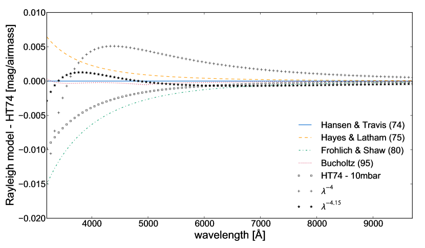
Figure 2: Comparison between different methods to model the Rayleigh scattering in the SNIFS wavelength range from Hansen & Travis (1974) (blue), Hayes & Latham (1975) (yellow), Froehlich & Shaw (1980) (green) and Bucholtz (1995) (red). The comparison is made for the mean pressure at the Mauna Kea summit (616 mbar). The discrepancies between the different models are less than 1.5% over the wavelength range considered in this paper.

Fig. 2 shows other numerical evaluations of the Rayleigh scattering for a Mauna Kea mean pressure of 616 mbar, including Hansen & Travis (1974), Hayes & Latham (1975) and Froehlich & Shaw (1980) whose results are very similar to the model from Bucholtz (1995). Note that all these methods are very close to the simplified formula $\lambda^{-4+\epsilon}$, which is often found in the literature. In our analysis, the value of $\epsilon$ that best matches the Rayleigh description at aforementioned 616 mbar is $-0.15$ (cf. Fig. 2, solid black line).

Since we have a direct measurement of the surface pressure at the Mauna Kea summit at the time of our observations, the Rayleigh scattering component is not adjusted in our model. Rather, following common practice in the atmospheric science community we directly use the calculated Rayleigh extinction. For convenience we employ the Hansen & Travis (1974) description, very close to the Bucholtz (1995) expression.

4.1.2 Aerosol scattering

The monitoring of atmospheric aerosols is a fundamentally difficult problem due to its varying composition and transport by winds over large distances. For Mauna Kea we expect that aerosols of maritime origin, essentially large sea-salt particles, will dominate (Dubovik et al., 2002). In that case, we can expect a low aerosol optical depth given the elevation of Mauna Kea (Smirnov et al., 2001). Furthermore, the strong temperature inversion layer between 2000 and 2500 m over the island of Hawaii helps to keep a significant fraction of aerosols below the summit. Major volcanic eruptions can inject aerosols into the upper atmosphere, affecting extinction (Rufener, 1986; Vernier et al., 2011). Nearby Kilauea has been active throughout the period of our observations, but its plume is generally capped by the inversion layer and carried to the southwest, keeping the plume well away from the Mauna Kea summit.

The particle sizes are of the order of the scattered wavelength for the wavelength range (3000–10000 Å) of our study. According to Ångström (1929), Ångström (1964) and Young (1989), and in agreement with the Mie theory, the chromaticity of the aerosol scattering is an inverse power law with wavelength:

$$k_{A}(\lambda)=\tau\times(\lambda/1\;\mu\mathrm{m})^{-\aa}$$ (10)

where $\tau$, the aerosol optical depth at 1 $\mu$m, and $\aa$, the Ångström exponent, are the two parameters to be adjusted.

According to Reimann et al. (1992), the value of the exponent $\aa$ varies between $4$ and $-2$ for astronomical observations, depending on the composition of the aerosol particles. We will see in § 8.2 that the Ångström exponent at the Mauna Kea summit is confirmed to vary within these values, with a mean value close to 1. While aerosol scattering may be spatially and temporally variable, since it is anticipated to be weak at the altitude of Mauna Kea we begin our study by assuming aerosol scattering is constant on the timescale of a night. We defer the discussion of this hypothesis to § 9.3.

4.1.3 Water scattering in clouds and grey extinction

The water droplets and ice crystals in clouds also affect the transmission of light through the atmosphere. To first approximation, it can be assumed that the size of the constituents of the clouds are large compared to the wavelength of the incident light (a cloud droplet effective radius is of the order of at least 5 $\mu$m, Miles et al. 2000). In this case, the dominant phenomenon is the refraction inside water droplets. The extinction is then almost independent of wavelength and can be considered achromatic. We will therefore refer to this extinction as “grey extinction”. In § 7.6 we will examine this approximation more closely, and demonstrate is applicability for cloud conditions under which useful astronomical observations are possible.

In our current framework, extinction by clouds is the only component treated as variable on the time scale of a night (cf. § 9). It is represented by the atmospheric transmission variation parameter, $\delta T(\lambda,\hat{z},t)$. Being grey, there is no wavelength dependence, and we may write:

$$\delta T(\lambda,\hat{z},t)=\delta T(\hat{z},t).$$ (11)

4.2 Molecular absorption

The molecular absorption bands and features in the atmosphere are essentially due to water vapor, molecular oxygen, and ozone. Nitrogen dioxide exhibits broad absorption, but is too weak to affect astronomical observations (Orphal & Chance, 2003). The regions below 3200 Å and above 8700 Å are especially afflicted, due to strong $\mathrm{O_{3}}$ and $\mathrm{H_{2}O}$ absorption, respectively.

4.2.1 Ozone bands

The ozone opacity due to the Hartley & Huggins band (Huggins, 1890) is responsible for the loss of atmospheric transmission below 3200 Å and the Chappuis band (Chappuis, 1880) has a non-negligible influence — at the few percent level — between 5000 Å and 7000 Å.

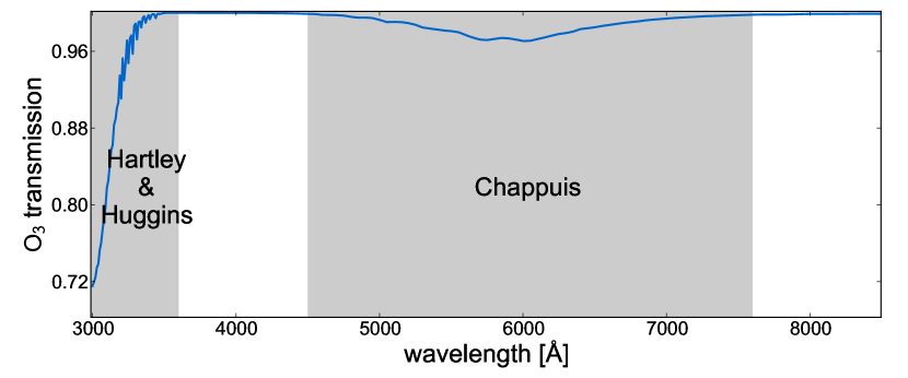
Figure 3: Ozone transmission template of the Hartley & Huggins band in the UV and the Chappuis band at 6000 Å.

In order to model the ozone absorption we are using a template (cf. Fig. 3) for which we adjust the scale:

$$k_{\mathrm{O_{3}}}(\lambda)=I_{\mathrm{O_{3}}}\times P_{\mathrm{O_{3}}}(\lambda)$$ (12)

where $P_{\mathrm{O_{3}}}(\lambda)$ represents the ozone extinction template computed using the MODTRAN library and $I_{\mathrm{O_{3}}}$ is a scale factor, expressed in Dobson Units [DU].

4.2.2 Telluric lines

In contrast to the other extinction components, the telluric lines affect only a few limited wavelength ranges. The major features are comprised of saturated narrow $\mathrm{O_{2}}$ lines, including the Fraunhofer “A” and “B” bands, deepest at 7594 Å and 6867 Å respectively, a wide $\mathrm{H_{2}O}$ band beyond 9000 Å, and $\mathrm{H_{2}O}$ absorption features in several spectral regions between 6000 Å and 9000 Å. The weak O₄ features at 5322 Å and 4773 Å (Newnham & Ballard, 1998) have been neglected in our current treatment. Table 1 shows the wavelength ranges taken to be affected by telluric features for purposes of SNfactory calibration. These wavelength ranges were determined from the high resolution telluric spectrum from Kitt Peak National Observatory (KPNO, Hinkle et al., 2003), matched to the SNIFS resolution.

Table 1: Wavelength ranges of telluric features, determined from the high resolution KPNO spectrum, matched to the resolution of SNIFS (3.2 Å for the red spectroscopic channel).

Feature	Start	End
	[Å]	[Å]
$\mathrm{O_{2}}\gamma+\mathrm{O_{4}}$	6270.2	6331.7
$\mathrm{O_{2}}$ B	6862.1	6964.6
$\mathrm{H_{2}O}$	7143.3	7398.2
$\mathrm{O_{2}}$ A	7585.8	7703.0
$\mathrm{H_{2}O}$	8083.9	8420.8
$\mathrm{H_{2}O}$	8916.0	9929.8

For the telluric lines, the airmass dependence, $\rho$, from Eq. (7) corresponds to a saturation parameter. Since the telluric contributions are separated enough to be interpolated over, it is possible to determine this saturation parameter, which according to Wade & Horne (1988); Stubbs et al. (2007) is approximately 0.5 for strongly saturated lines and 1 for unsaturated lines. In § 6.1 we will further discuss the value of $\rho$ for the telluric lines as well as the method used to correct them.

5 Nightly photometricity

The photometricity of a night refers to its transmission stability in time. At the present time we are only able to separate nights with clouds from those unlikely to have clouds. Besides clouds, the aerosol and water absorption components of the extinction are the most variable. However, because their variation is difficult to detect, we do not currently include these components when assessing the photometricity of a night. Recall that our formalism and instrument capabilities allow us to determine the extinction on both photometric and non-photometric nights. Nights that are non-photometric simply use estimates of $\delta T_{i}(\lambda,\hat{z},t)$ obtained from the parallel imaging channel. For this reason we can afford to be conservative in our selection of photometric nights.

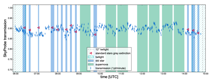
(a) Photometric night

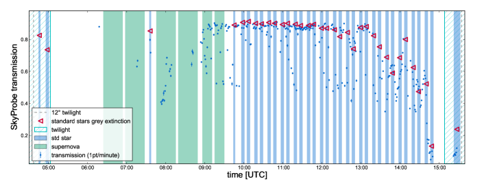
(b) Non-photometric night

Figure 4: LABEL:sub@fig:skyprobe-phot SkyProbe atmospheric transparency (blue points) and SNIFS standard stars grey extinction term $\delta T$ (red triangles) for a photometric night and LABEL:sub@fig:skyprobe-nonphot a non-photometric night.

5.1 SkyProbe

In order to obtain a reliable assessment of the sky transparency stability, we use several available sources. These include SkyProbe (Cuillandre et al., 2002; Steinbring et al., 2009), photometry from the SNIFS parallel imager, the brightness stability of the SNIFS guide stars, the scatter of our standard stars about the best extinction solution, and knowledge of technical issues such as dome slit misalignment.

Because of its high cadence and continuity across the sky, we begin with measurements from SkyProbe (Cuillandre et al., 2002; Steinbring et al., 2009), a wide field camera mounted at the CFHT and dedicated to real time atmospheric attenuation analysis. Some outlier cleaning of the SkyProbe data is necessary since it includes measurements taken when the telescope is slewing. There also is evidence for occasional small but highly stable offsets between pointings, suggestive of small systematics in the photometry reference catalog or photometry technique employed. The robustness of such cleaning is adversely affected on nights when CFHT slews frequently between fields. We find that generally when the SkyProbe data stream has an RMS greater than 3.5% after cleaning the night is not likely to be photometric. One added limitation of our use of the SkyProbe data is the possibility that CFHT could miss the presence of clouds if only part of the sky is affected throughout the night.

5.2 Guide star

Since the guiding video and resultant brightness measurements of SNIFS guide stars are stored for all guided observations, the presence of clouds in the SNIFS field can be ascertained directly. Some cleaning is needed for these data as well, since cosmic ray hits or strong seeing variations can produce measurable fluctuations in the guide star photometry. The guide star video has a rate between 0.4 and 2 Hz, so the data can be averaged over 30–60 sec intervals to achieve sensitivity at the few percent level for most guide stars. As different guide stars from the different targets observed over the course of a night have different and unknown brightnesses, these data can only detect relative instability over the interval of an observation but not between observations and with poor sensitivity for short exposures.

5.3 Tertiary reference stars

For fields that are visited numerous times, field stars in the SNIFS photometric channel can provide an estimate of the average attenuation over the course of the parallel spectroscopic exposure. We refer to these as a “multi-filter ratio” or MFR. The SNIFS spectroscopic and imaging channels cover adjacent regions of sky spanning just a few arcminutes, and sit behind the same shutter. Pereira (2008) found that this relative photometry is accurate to $\sim 2$%, except for the rare cases where there are few suitable field stars. For long exposures of supernovae there generally are enough field stars with high signal-to-noise. Some standard star fields lack enough stars to ensure a sufficient number of high signal-to-noise field reference stars for our typical exposure times and under mildly cloudy conditions. Use of such standards for our program has been phased out.

5.4 Spectroscopic standard stars

Finally, our formalism allows us to easily compute an initial instrument calibration and extinction curve under the assumption that a night is non-photometric. The resulting values of $\delta T(\hat{z},t)$ can then be used to detect the presence of clouds during the standard star exposures themselves.

5.5 Combined probes

Combining all this information, we estimate the photometricity of the night for the targets observed by SNIFS. It is important to consider the noise floor for each source to avoid rejecting too many photometric nights. By examining the distribution of each photometricity source we are able to define two thresholds, “intermediate” and “non-photometric”. For our purposes in this paper, non-photometric nights are defined as having at least one source above a non-photometric threshold, or all sources above the intermediate thresholds. The threshold values are listed in Table 2.

Table 2: Root Mean Square thresholds (in %) for the different photometricity source distributions. For values intermediate between the photometric and non-photometric thresholds, a combination of indicators is used to ascertain the temporal stability of the atmospheric transmission.

Sources	Photometric	Non-photometric
SkyProbe	$<2.5$	$>3.5$
SNIFS guide star	$<2.5$	$>5$
SNIFS photometry	$<2.5$	$>4$
SNIFS standard stars	$<2.5$	$>4$

Examples of the SkyProbe transmission are shown in Fig. 4a for a photometric night and Fig. 4b for a non-photometric night. The red triangles represent the grey extinction term, $\delta T_{i}(\hat{z},t)$, for each standard star $i$ observed during the night. The pattern of the grey extinction seen in Fig. 4b follows that of the independent SkyProbe data (blue points). This confirms that the parameter $\delta T(\hat{z},t)$ is able to track atmospheric attenuation by clouds (cf. Fig. 5 to see the distribution of $\delta T(\hat{z},t)$ in non-photometric conditions). We estimate that $\sim 35\%$ of the SNfactory nights were photometric according to these transmission stability cuts. This value is lower than values of 45–76% that have been reported elsewhere (Schöck et al. 2009 & ESO Search for Potential Astronomical Sites, ESPAS), however as noted earlier, for our purposes in this paper we wish to set conservative photometricity criteria.

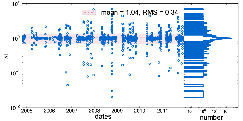
Figure 5: Distribution and histogram of the grey transmission parameter $\delta T$ for each observed standard star during non-photometric conditions. Note that many non-photometric nights have only thin clouds, and therefore $\delta T\sim 1$.

6 Extinction from standard star observations

In the case of standard star observations, $S^{\star}(\lambda,t)$ is known a priori as a tabulated reference, $\overline{S}(\lambda)$, and thus the term on the left side of Eq (6) becomes a known quantity. To solve for the extinction and instrument calibration we begin by constructing a conventional $\chi^{2}$:

$$\chi^{2}=\sum_{i}\mathcal{R}_{i}\cdot V_{i}^{-1}\cdot\mathcal{R}_{i}^{\text{T}},$$ (13)

where the index $i$ stands for each individual standard star, $V_{i}$ is the covariance matrix (described below) and $\mathcal{R}_{i}$ represents the residuals, given by,

$$\mathcal{R}_{i}=\log C(\lambda)-0.4\times K_{\mathrm{atm}}(\lambda,\hat{z})+\log\delta T_{i}(\hat{z},t)-\log\frac{S_{i}(\lambda,\hat{z},t)}{\overline{S}_{i}(\lambda)}.$$ (14)

$K_{\mathrm{atm}}(\lambda,\hat{z})$ represents the parametrization detailed in § 4 for the Rayleigh, aerosols, ozone and telluric extinction components. The only adjustable parameters are:

• $C(\lambda)$, the instrument calibration (cf. Eq. 2),

• $\aa$ and $\tau$, the aerosol Ångström exponent and optical depth,

• $I_{\mathrm{O_{3}}}$, the ozone template scale factor,

• $\delta T_{i}(\hat{z},t)$, the transmission variation for each standard star $i$.

$k_{R}(\lambda)$ is not adjusted since it depends only on the surface pressure $P$, which is known a priori. The instrument calibration, $C(\lambda)$, and the atmospheric extinction, $K_{\mathrm{atm}}(\lambda,\hat{z})$, are spectrally smooth, so we do not constrain the model at full resolution. Rather, we employ a coarser spectral grid, consisting of “meta-slices”; we construct meta-slices for each of the two SNIFS channels, with meta-slice widths between 100 and 150 Å depending on the channel. The telluric line scale factors must also be determined, but we will see in the following section that this can be accomplished in a separate step.

$V_{i}$ in Eq. 13 is the covariance matrix between all meta-slice wavelengths of standard star $i$ for a given night; this assumes the covariance between standards is zero. To build the covariance matrix of each standard star, we first include the statistical covariance issued from the point-source PSF-extraction procedure. A constant is then added to the whole matrix, representing a 3% correlated error between all meta-slices for a given standard star observation. This is added as a way to approximate our empirically determined per-object extraction error.

As described in § 6.2.1, when solving for the instrument calibration and extinction we will modify Eq. 13 to include Bayesian priors on some atmospheric parameters.

6.1 Telluric correction

The telluric lines affect only limited wavelength regions, whereas the other atmospheric extinction components are continuous (aerosol and Rayleigh scattering) or very broad (ozone). Although it is possible to fit the telluric lines at the same time as the extinction continuum, we chose to do it in a separate step both for historical implementation reasons and to allow a telluric correction when the flux calibration is not needed. As a consequence, with our approach the telluric wavelength regions can be either avoided for the study of the atmospheric extinction continuum or corrected separately using standard stars to determine an average correction spectrum per night. In the latter case we separate $K_{\mathrm{atm}}(\lambda,\hat{z})$ as follows:

$$K_{\mathrm{atm}}(\lambda,\hat{z})=\underbrace{X(\hat{z})\times\left(k_{R}(\lambda)+k_{A}(\lambda)+k_{\mathrm{O_{3}}}(\lambda)\right)}_{K(\lambda,\hat{z})}+X^{\rho}(\hat{z})\times k_{\oplus}(\lambda).$$ (15)

For a standard star $i$ on a given night,

$$\mathscr{C}^{\star}_{i}(\lambda,\hat{z},t)=\frac{S_{i}(\lambda,\hat{z},t)}{\overline{S}_{i}(\lambda)}=\delta T_{i}(\hat{z},t)\times C(\lambda)\times 10^{-0.4\times K(\lambda,\hat{z})},$$ (16)

behaves as a smooth function of wavelength, which can be reasonably well modeled with a spline $\mathscr{C}(\lambda,\hat{z},t)$, outside the telluric lines regions. Inserting this into Eq. (6) for standard stars gives:

$$\log\frac{S_{i}(\lambda,\hat{z},t)}{\overline{S}_{i}(\lambda)}=\log\mathscr{C}_{i}(\lambda,\hat{z},t)-0.4\times X_{i}^{\rho}(\hat{z})\times k_{\oplus}(\lambda).$$ (17)

As shown in § 4, the amplitude of the telluric lines is proportional to the factor $X^{\rho}(\hat{z})$. Taking the logarithm of Eq. (17), we obtain a linear expression with respect to the logarithm of the airmass, $\log X(\hat{z})$, allowing us to fit for the saturation factor $\rho$ and the telluric extinction $k_{\oplus}(\lambda)$:

$$\log\left(-2.5\times\log\frac{S_{i}(\lambda,\hat{z},t)/\overline{S}_{i}(\lambda)}{\mathscr{C}_{i}(\lambda,\hat{z},t)}\right)=\log k_{\oplus}(\lambda)+\rho\times\log X_{i}(\hat{z}).$$ (18)

Optically thin absorption produces attenuation proportional to the airmass ($\rho=1$) whereas highly saturated lines are expected to have equivalent widths growing as the square root of the airmass ($\rho=0.5$). According to the observations performed by Wade & Horne (1988) for airmasses from 1 to 2, the saturated Fraunhofer “A” and “B” lines and the water lines have an airmass dependence $\rho\simeq 0.6$. We repeated their approach and fit for $\rho_{\mathrm{O_{2}}}$ and $\rho_{\mathrm{H_{2}O}}$ for each observation night. The saturation distributions are shown in Fig. 6. We find a median value of 0.58 for $\rho_{\mathrm{O_{2}}}$, and find a normalized Median Absolute Deviation (nMAD) of 0.03. As for the $\mathrm{H_{2}O}$ lines, since the water content in the atmosphere is variable, so is the saturation parameter $\rho_{\mathrm{H_{2}O}}$. We found median values of $0.60\pm 0.27$ and $0.35\pm 0.37$ for water regions below and above $\approx 9000$ Å, respectively.

The latter result for the strong $\mathrm{H_{2}O}$ absorption region (8916–9929 Å) is treated independently from the region below $\approx 9000$ Å since it cannot be measured very well. This is because the wavelength range of this particular band extends beyond the SNIFS wavelength range, which makes the estimation of the spline fit for $\mathscr{C}$ unreliable. As we can see in Fig. 7, the “strong” water telluric band is difficult to correct in these conditions. Nevertheless, by fixing the saturation parameter, a correction accurate to 5–10% can still be obtained.

Subsequently, and in order to improve the fit, we choose to neglect the variations of the saturation and we fix $\rho_{\mathrm{O_{2}}}=0.58$ for the molecular oxygen absorption and to $\rho_{\mathrm{H_{2}O}}=0.6$ for the water vapor absorption (as did Wade & Horne, 1988). Neglecting the saturation variations for the water bands has no perceptible negative impact on the quality of the telluric correction since there is still a degree of freedom from the telluric scale factor.

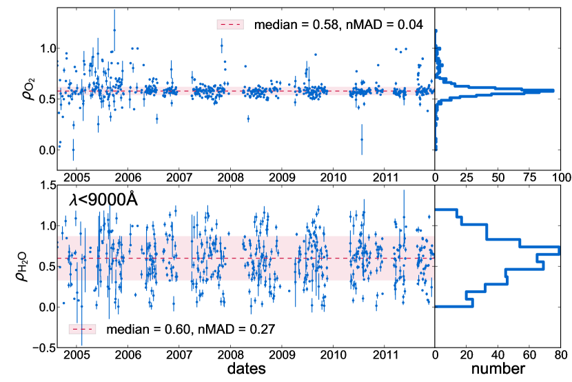
Figure 6: Distributions of the saturation parameters, $\rho_{\mathrm{O_{2}}}$ and $\rho_{\mathrm{H_{2}O}}$, for each night of the SNfactory data set. The water lines above 9000 Å are treated separately due to the difficulties encountered in the correction of the “strong” $\mathrm{H_{2}O}$ telluric band. One reason we chose to fix the water saturation parameter is that some fits gave unphysical values (e.g. $\rho_{\mathrm{H_{2}O}}>1$).

After removing the pseudo-continua, $\mathscr{C}(\lambda,\hat{z},t)$, from the spectra, linear fits of the intensity are performed for each group of lines of the SNfactory derived telluric template (i.e. $\mathrm{O_{2}}$ and $\mathrm{H_{2}O}$) with their respective saturation parameter fixed.

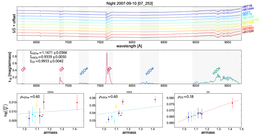
Figure 7: Example of a telluric correction spectrum computation for a typical night. Top panel: All the reference normalized standard star spectra $S/\overline{S}$ of the night and their continua $\mathscr{C}$ (dashed lines). Middle panel: Adjusted telluric template intensities as function of their saturation. Bottom panels: Dependence with respect to airmass of $\log S/\overline{S}-\log\mathscr{C}$ integrated over each group of lines (shaded areas in middle panel). The dashed lines represent the airmass dependence with a fixed saturation exponent.

The results of the linear fit for $k_{\oplus}(\lambda)$ from a given night are shown on Fig. 7. The first panel shows each observed spectrum divided by its corresponding intrinsic spectrum (solid lines), together with the pseudo-continuum $\mathscr{C}(\lambda,\hat{z},t)$ (dashed lines) which is a global fit for $S/\overline{S}$ in which the telluric regions are excluded. The resulting telluric correction template is presented in the second panel. The linear fits for each group of lines are shown in the three bottom panels. We use $\mathrm{H_{2}Os}$ to denote the strong $\mathrm{H_{2}O}$ telluric lines redward of 9000 Å, and $\mathrm{H_{2}Ow}$ to denote the weaker $\mathrm{H_{2}O}$ telluric lines blueward of this. In the middle bottom panel we see that the $\mathrm{H_{2}Os}$ correction is poorly constrained due to the large scatter, as expected. (We eventually expect to improve this situation by extending the spectral extraction beyond 1 $\mu$m.)

The current accuracy of the telluric correction is generally at the same level as the noise of the spectra, and thus sufficient for rigorous spectral analysis, including studies of spectral indicators (Bailey et al., 2009; Chotard et al., 2011). For the oxygen lines, which are very narrow, some wiggles ($\sim 2$% peak to peak fluctuations) can remain after the correction in a few cases due to small random wavelength calibration offsets (of the order of $\sim 0.1$ Å) between the spectra and the template.

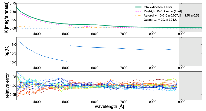
Figure 8: Upper panel: Atmospheric extinction, $K(\lambda)$ (solid line), for a given non-photometric night (2010-06-28); i.e. the sum of its physical components, Rayleigh scattering $k_{R}(\lambda)$ (dashed line), aerosol scattering $k_{A}(\lambda)$ (dash-dot line) and ozone absorption $k_{\mathrm{O_{3}}}(\lambda)$ (dotted line). Middle panel: instrument calibration $C(\lambda)$; this includes not only the overall throughput, but also scaling by the spectral flat field. Bottom panel: Relative error of the standard star fluxes after the fit (i.e. the difference between the individual standard star flux solutions and $\log C(\lambda)$). The grey bands in all three panels indicate meta-slices that are affected by the “strong” $\mathrm{H_{2}O}$ telluric features. This wavelength region is not used when fitting for the other physical components.

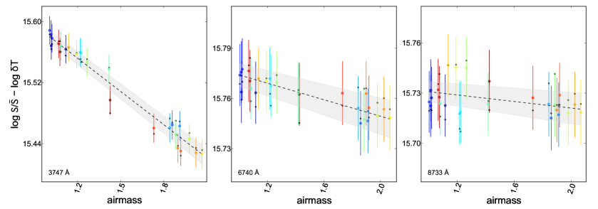
Figure 9: Linear fit of $\log S/\overline{S}-\log\delta T$ with respect to the airmass for three different wavelengths (indicated by dashed lines in the top panel), where each point represents a star with (large points with error bars) or without (small points) grey extinction correction. The dashed lines represent the linear fits and the grey bands their corresponding error.

6.2 Nightly atmospheric extinction solutions

6.2.1 Introduction of Bayesian priors

Outside of the telluric lines, or after correction of the telluric features, Eq. (6) for standard stars becomes:

$$\log\frac{S_{i}(\lambda,\hat{z},t)}{\overline{S}_{i}(\lambda)}=\log C(\lambda)-0.4\times X_{i}(\hat{z})\times K(\lambda)+\log\delta T_{i}(\hat{z},t).$$ (19)

Under these conditions, a degeneracy appears in Eq. (19) between the instrument calibration $\log C(\lambda)$ and the average of the grey extinction parameters $\langle\log\delta T_{i}\rangle$. This means that the value of $C(\lambda)$ and the geometric average of the $\delta T_{i}$ values will only be relative measurements during non-photometric nights. The absolute scale of the $\delta T_{i}$ can be determined independently though using MFRs obtained by secondary stars from the SNIFS photometric channel. Such MFRs are not needed to compute the atmospheric extinction, but we refer the interested reader to Pereira (2008) and Scalzo et al. (2010) for further description of this particular step of the SNIFS flux calibration process.

This degeneracy can be lifted during the fit by setting the mean value of the grey extinction parameter to an arbitrary value. For a photometric night there should be no need for a grey extinction term ($\delta T_{i}\equiv 1$), thus $\langle\log\delta T_{i}\rangle$ would be zero if such a term were included. To ease comparisons between photometric and non-photometric nights, or the effects of changing the photometric status of a night, we therefore set the mean value of the cloud transmission to 1 on non-photometric nights. Since often such nights have only thin cirrus or clear periods, this can provide meaningful information on cloud transmission for other types of studies. Note that mathematically the 3% correlated error put into the covariance matrix, $V$, can be traded off against the grey extinction term on non-photometric nights. However, this has no effect on the photometric solution.

In addition, in order to ensure that all components behave physically, we chose to also apply priors to the aerosol and ozone parameters. This choice is motivated by the fact that degeneracies can appear between the physical components in some wavelength ranges resulting in negative extinction or poor numerical convergence (For example, on non-photometric nights there is a degeneracy between $\delta T$ and $\tau\sim\lambda^{0}$). All priors are Gaussian, but we chose to set a prior on the logarithm of the aerosol optical depth since this provides a better match to the aerosol optical depth distribution (cf. Fig. 19b) at the atmospheric observatory on nearby Mauna Loa. All priors are summarized in Table 3, and they are implemented by adding a penalty function to the $\chi^{2}$ of Eq. (13):

$$\chi^{2}_{\mathrm{total}}=\chi^{2}+\Psi^{2}$$ (20)

where the priors on the atmospheric extinction shape are encapsulated in the penalty function,

$$\Psi^{2}=\left(\frac{I_{\mathrm{O_{3}}}-{I^{\star}_{\mathrm{O_{3}}}}}{\sigma^{\star}_{I_{\mathrm{O_{3}}}}}\right)^{2}+\left(\frac{\aa-\aa^{\star}}{\sigma^{\star}_{\aa}}\right)^{2}+\left(\frac{\ln(\tau/\tau^{\star})}{\varsigma^{\star}_{\tau}}\right)^{2}.$$ (21)

The extinction for a given night is obtained by minimizing Eq. (20) for all std stars $i$, and all (meta-slices) wavelengths $\lambda$.

Table 3: List of priors used in the fit for the atmospheric extinction and their corresponding errors. Their goal is to ensure physical behavior of the extinction components.

Prior	Value		Scaling
$I^{\star}_{\mathrm{O_{3}}}$	260 $\pm$	50 DU	linear
$\tau^{\star}$	0.007 $\pm$	80%	logarithmic
$\aa^{\star}$	1 $\pm$	3	linear

6.2.2 Maximum-likelihood fitting

The total $\chi^{2}$ (Eq. (20)), that includes the Bayesian penalty function $\Psi^{2}$ is minimized. Consequently, the resulting error on the parameters is computed by inverting the covariance matrix of the full function.

The different contributions to the resulting extinction fit for a specific night are illustrated in Fig. 8, along with the instrument calibration. The noticeable larger scatter in the blue arm can be explained by the PSF model used for point-source extraction which is presumably less accurate in the blue than in the red, because of a stronger chromaticity; this is even more evident for the short exposure PSF model used for bright standard stars, due to the complex PSF in short exposures. Overall, increased errors in point-source extracted spectra in the blue will contribute to a larger scatter in the flux calibration residuals. Linear relations are adjusted for three distinct wavelength bins from the same night in the Fig. 9. In this example the night is slightly non-photometric and the grey attenuation has a RMS of the distribution of the order of 4% (cf. Fig. 10 for a distribution of the $\delta T_{i}(\hat{z},t)$ in airmass and in time). Finally, the covariance map of all the adjusted parameters of the night is presented in Fig. 11.

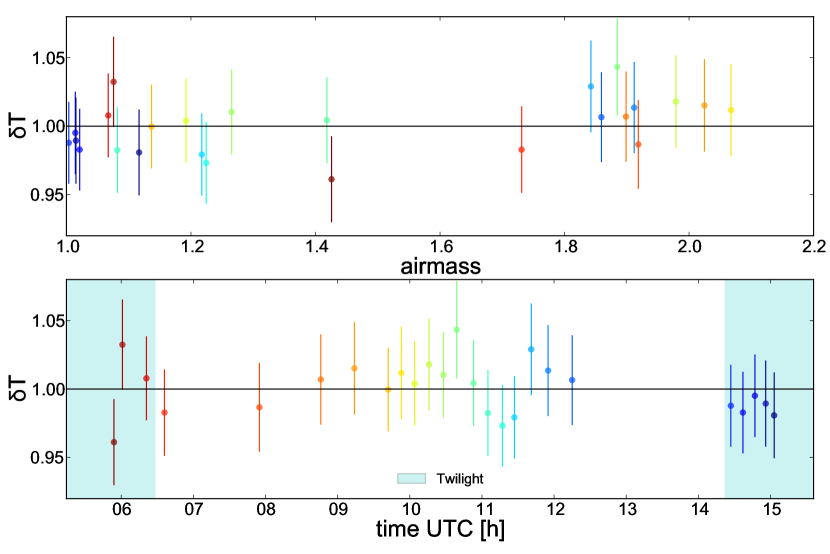
Figure 10: The grey extinction distribution, $\delta T(\hat{z},t)$, for a slightly non-photometric night (2010-06-28). The top panel shows $\delta T(\hat{z},t)$ as a function of airmass while the bottom panel shows $\delta T(\hat{z},t)$ as a function of time. Since the night is non-photometric most of the scatter is due to clouds, but there is some scatter due to achromatic extraction errors. Recall that we normalize by the mean of $\delta T(\hat{z},t)$ rather than the largest (fewest clouds) value.

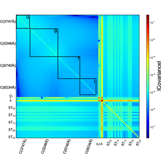
Figure 11: Resulting covariance matrix of the parameters for a given non-photometric night (2010-06-28). The represented parameters are the flux solution $C(\lambda)$ at every meta-slice wavelength, the atmospheric normalized model parameters $I_{\mathrm{O_{3}}}$, $\tau$ and $\aa$ as well as the grey extinction $\delta T$ per star. SDSS filters u, g, r and i are also represented (black squares) over the flux solution wavelengths.

The 478 extinction curves computed using this method are presented in Fig. 12. Individual nights are plotted in light grey whereas the median extinction, based on the median physical parameters, is represented by the thick solid green line. The green band represents the dispersion of the nightly extinction determinations. Fig. 13 shows the correlations between all extinction parameters for both photometric and non-photometric nights. No obvious correlations appear between the parameters except for $\tau$ and $\aa$, which are expected to be correlated since in combination they represent the aerosol component of the extinction. This demonstrates the independent behavior of the physical components.

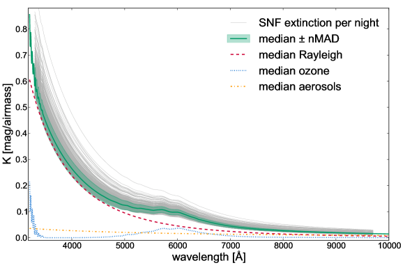
Figure 12: Typical extinction and its variability over the 7 years of the observation campaign. The superposition of all nightly extinction curves (grey) is shown, along with the median Mauna Kea extinction we derive (green).

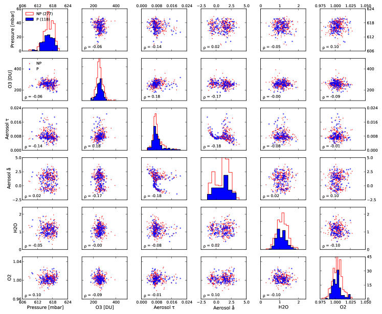
Figure 13: Correlations between extinction parameters for both photometric (blue circles) and non-photometric nights (red points). No strong correlations are seen between pressure, ozone, or telluric $\mathrm{H_{2}O}$ and $\mathrm{O_{2}}$. The aerosol parameters $\tau$ and $\aa$ are correlated because they represent the same physical component. The distributions of the parameter values (diagonal plots) also are similar on photometric and non-photometric nights. Note that the incidence of aerosol exponents near $\aa\sim 0$ is suppressed on non-photometric nights since the grey extinction term can completely compensate for this case.

7 Accuracy and variability

Having presented the fitting methodology and median results, we will now discuss the accuracy of the results and what can be said about the variability of the various physical components.

7.1 Extinction accuracy

The 478 extinction error spectra are shown in Fig. 14. These curves represent our ability to measure the extinction with the standard observations taken each night. This is largely set by the numbers of standard stars and their airmass range. These curves do not represent natural variations in the extinction, which are addressed below. The mean error, displayed as a green line in the figure, decreases from its maximal value of 20 mmag/airmass in the UV to 7 mmag/airmass in the red. This power law behavior can be explained by the fact that the aerosol component is the main source of variability allowed in our model. A similar behavior is observed for all the individual error spectra (light grey curves) with various values of the power exponent. On nights with few standards or a small airmass range, the errors are larger. On such nights, use of the median extinction curve rather than the nightly curve should provide better calibration.

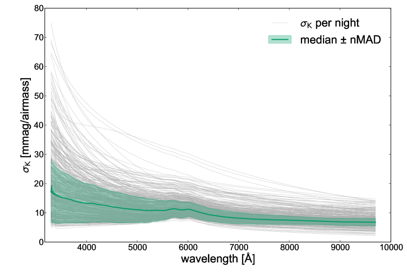
Figure 14: Error on the nightly extinction computations as a function of wavelength (light grey lines). The mean error and RMS of the extinction curves distribution are shown in green.

7.2 Rayleigh variability

The average Rayleigh extinction component is shown in Fig. 15a. During the course of the observations the surface pressure at the summit of Mauna Kea showed a peak-to-peak variation of 6 mbar around the average 616 mbar value. The nMAD of the variation was 2 mbar, which corresponds to an extinction variation of 2 mmag/airmass at the blue edge of our spectral range. The peak-to-peak extinction variation still would be only 6 mmag/airmass. These variations are negligible with respect to the aerosol or ozone components and have no impact on the global extinction variability at our required level of accuracy.

7.3 Aerosol variability

The median aerosol component we derive is shown in Fig. 15b, superimposed on our aerosol measurements from each night. Fortunately the median value is very low, ranging from $\sim$40 down to $\sim$10 mmag/airmass over the SNIFS wavelength range. Even so, aerosol variations are the largest contributor to the variability of the extinction continuum from one night to another, and these variations are also shown in Fig. 15b. The combined fluctuations in $\tau$ and the Ångström exponent are responsible for variations that reach an extreme of 0.4 mag/airmass at 3300 Å. It should be noted that SNIFS is not operated when winds exceed 20 m/s, so there may be more extreme aerosol excursions that our data do not sample.

7.4 Ozone variability

The mean ozone component we derive is shown in Fig. 15c, superimposed on our ozone measurements from each night. Over the Big Island the mean is 260 DU, a value lower than the world-wide mean. The maximal peak to peak ozone variability in one year can reach 60 to 80 DU. Much of this variation is scatter around a clear seasonal trend attributable to the Quasi-Biennial Oscillation (QBO), which has a mean amplitude around 20 DU. Much of the remaining variation is due to tropospheric winds (Steinbrecht et al., 2003). 20 DU is only a 8% variation, corresponding to 4 mmag/airmass for the ozone peak at 6000 Å. We will show in § 8.1, this level of variation currently is very difficult for us to detect. While this level of uncertainty is unimportant for our science program, we could better constrain ozone by using the SNIFS standard star signal available below 3200 Å, where the Hartley & Huggins band is much stronger.

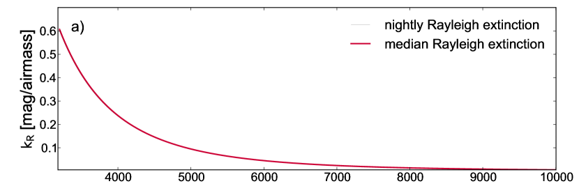
(a)

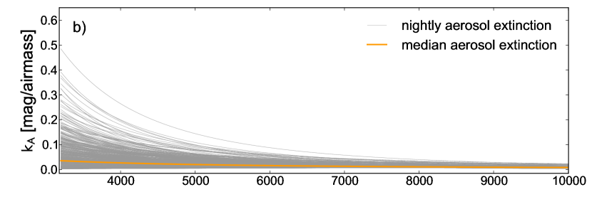
(b)

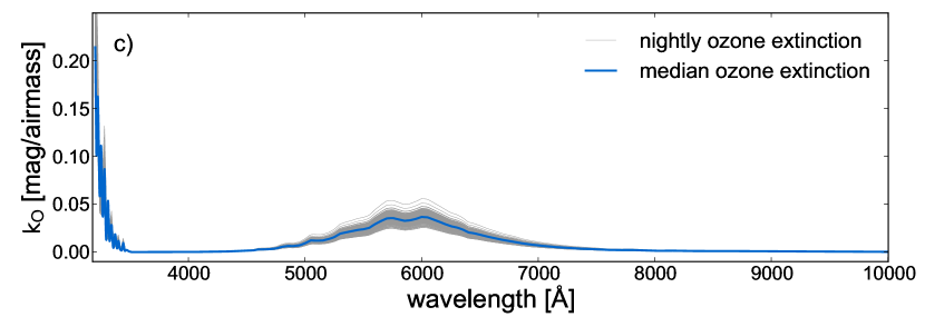
(c)

Figure 15: Nightly contributions of each physical component of the continuum extinction, showing their mean value and variability during the course of our observing campaign. All the nightly Rayleigh extinction curves (in grey) are within the width of the red median curve.

7.5 Telluric line variability

The strength of the $\mathrm{O_{2}}$ and $\mathrm{H_{2}O}$ telluric features is displayed in Fig. 16. The fluctuations of the strength of the $\mathrm{O_{2}}$ lines are remarkably small. This is fortunate given the strength of the $\mathrm{O_{2}}$ A and B bands. On the other hand the strengths of the $\mathrm{H_{2}O}$ lines vary widely. For some nights our current practice of assuming a fixed $\mathrm{H_{2}O}$ strength for the entire night may be too simplistic. However, Mauna Kea has less Precipitable Water Vapor than most ground-based astronomical sites, and so far we have not encountered any serious problems with this approximation. We explore this question further in § 8.3.

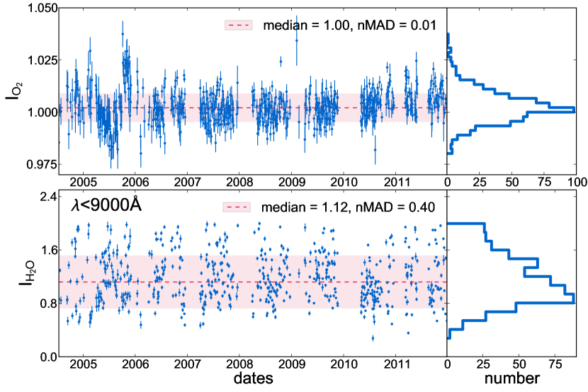
Figure 16: Distribution of the telluric strength over the SNfactory data set for each group of features. The strength represents the multiplicative factor needed to scale the template to the observed telluric features, and as such has no units.

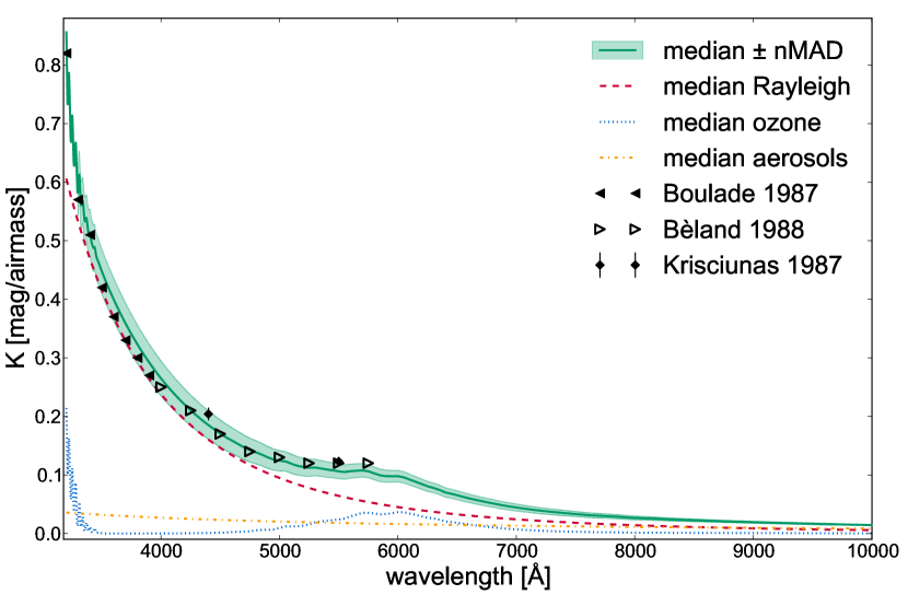
Figure 17: Mean SNfactory atmospheric extinction (solid line) and its physical components (dashed lines). For comparison we overplot the previous Mauna Kea extinction measures derived by Boulade (1987) (diamonds), Bèland et al. (1988) (triangles) and Krisciunas et al. (1987) (stars).

7.6 Short time variability

Due to our limited temporal sampling during each night, and the 2–3% achromatic scatter, it is difficult for us to detect extinction variability of less than 1% over the course of a night. As noted above, Rayleigh scattering variations are negligible, and ozone variations are nearly negligible with most of the variation occurring on seasonal timescales. Aerosol variations thus remain the primary concern for extinction variations during the night.

It should be noted that the $\delta T(\hat{z},t)$ term, used on photometric and non-photometric nights alike, is degenerate with aerosol extinction having an Ångström exponent of zero. Therefore, part of any temporal aerosol variation will be absorbed.

The GONG site survey of Mauna Kea (Hill et al., 1994b, a) found exceptional extinction stability. Mann et al. (2011) have demonstrated stability at the milli-magnitude level over the course of hours using SNIFS. Unfortunately, our extraction error is large enough (2 to 3%) to dominate our measurement of aerosol extinction variability (see Fig. 8 for typical errors). We have nevertheless tried to compare the mean aerosol extinction of time domains distributed at the beginning and the end of the night, but we have no evidence/indication whatsoever for a strong aerosol variation during the course of the night. Finally, the various metrics we used in § 5 to determine the photometric quality of each night are sensitive enough to alert us to transmission changes greater than several percent. If we are able to reduce the achromatic standard star extraction uncertainty, our sensitivity to temporal variations would also improve.

Turning to other sites, for Cerro Tololo in Chile Burke et al. (2010) showed that aerosol variations were rather small during a night. Burki et al. (1995) showed that for the La Silla site in Chile the total $U$-band extinction is correlated over a period of several days and that over one night the auto-correlation drops by only 5%. This implies a typical $\sim 2$% variation in extinction between the beginning and the end of the night. In our formalism the $\delta T(\hat{z},t)$ term can be used to test for such temporal trends on photometric nights. These sites have similar altitudes (2.1 km and 2.3 km, respectively), with inversion layers that are near (Burki et al., 1995; Gallardo et al., 2000) their summits. Since more aerosol variability might be expected for these sites than for Mauna Kea, this further justifies our assumption that nightly variability of aerosols is relatively unimportant for Mauna Kea.

8 Comparison to external measurements

As noted in the introduction, there have been previous measurements of the optical extinction above Mauna Kea, and we begin this section with a comparison of our results to those previous studies. Fig. 17 shows our median Mauna Kea extinction curve along with the observed fluctuations. Previous spectroscopic determinations, which covered only the blue half of the optical window, are overplotted as diamonds (Boulade, 1987) and stars (Bèland et al., 1988). The broadband filter extinction measurements from Krisciunas et al. (1987) are also shown (triangles). These external sources, taken more than 20 years prior, show excellent agreement with our own Mauna Kea extinction curve.

For further comparison we turn to atmospheric sciences data from Mauna Loa Observatory (MLO, Price & Pales, 1959, 1963), operated by the U.S. network Earth System Research Laboratory of the National Oceanic and Atmospheric Administration (NOAA). MLO is situated on the side of Mauna Loa mountain, 41 km south of Mauna Kea, at an altitude of 3400 m and 770 m below the summit. The observatory possesses specific instrumentation for aerosol and ozone measurements and we are particularly interested in comparing these measurements of ozone strength, aerosol optical depth and Ångström exponent with our own measurements obtained during nighttime on Mauna Kea.

8.1 Ozone comparison

The Total Column Ozone (TCO) in the region (i.e. the amount of ozone in a column above the site from the surface to the edge of the atmosphere) is measured at the MLO three times per day during week days using a Dobson spectro-photometer (Komhyr et al., 1997). The TCO comparison between Mauna Loa and SNfactory data is presented in Fig. 18.

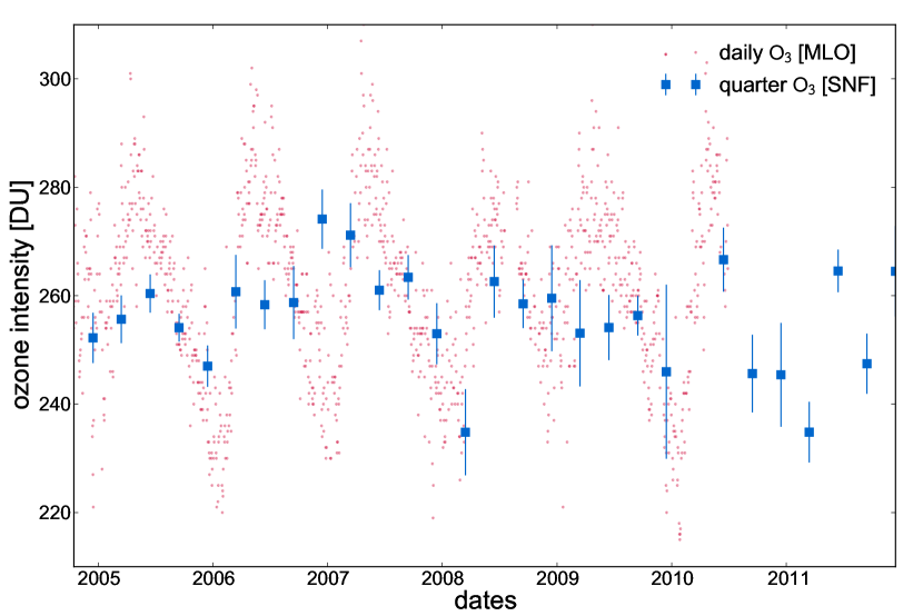
Figure 18: Total Column Ozone [Dobson units] from May 2004 to December 2011 for the SNfactory quarterly weighted averages (blue squares) and the Mauna Loa Observatory daily measurements (red points). The error bars on the SNfactory points represent the standard errors on the quarterly weighted averages.

The seasonal $\mathrm{O_{3}}$ variability is well established by the Mauna Loa data, with clear peaks corresponding to summer. The seasonal pattern observed in the SNfactory ozone variability is less obvious. This is due to our use of a prior. The typical nightly measurement uncertainty on $I_{\mathrm{O_{3}}}$ is around 60 DU without the prior. Given our prior with standard deviation 50 DU (see Table 3), the fit will return a value of $I_{\mathrm{O_{3}}}$ roughly midway between the true value and the mean of the prior (260 DU). This bias suppresses the amplitude we measure for the seasonal variation in ozone, but in the worst case leads to a spectrophotometric bias below 0.3%. If desired, this bias could be further minimized by using the Mauna Loa values as the mean for the prior on each night, or by first estimating a prior on a quarterly basis from our own data using an initial run without the prior, or by measuring $\mathrm{O_{3}}$ using SNIFS coverage of the Hartley & Huggins band below 3200 Å.

Overall, the behavior of our ozone measurements averaged over a quarter seems consistent with the Mauna Loa measurements although being not as accurate.

8.2 Aerosol comparison

The MLO ground-based aerosol data come from the AERONET (AErosol RObotic NETwork. Holben et al., 2001; Smirnov et al., 2001; Holben et al., 2003). AERONET uses wide angular spectral measurements of solar and sky radiation measurements. For these reasons, such aerosol measurements at Mauna Loa have only been carried out during daytime, and usable data requires reasonably good weather conditions (no clouds). Figures 19a and 19b show the comparisons between Mauna Loa data and SNfactory data for the Ångström exponent and the optical depth of the aerosol.

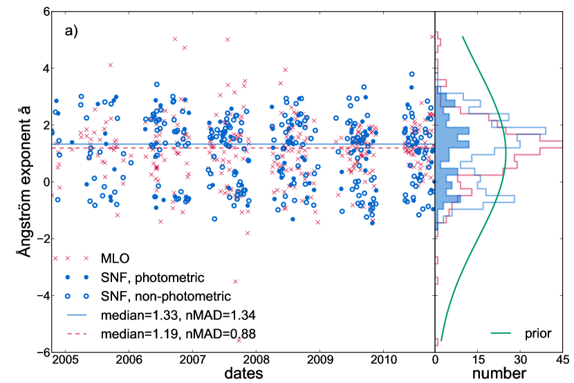
(a)

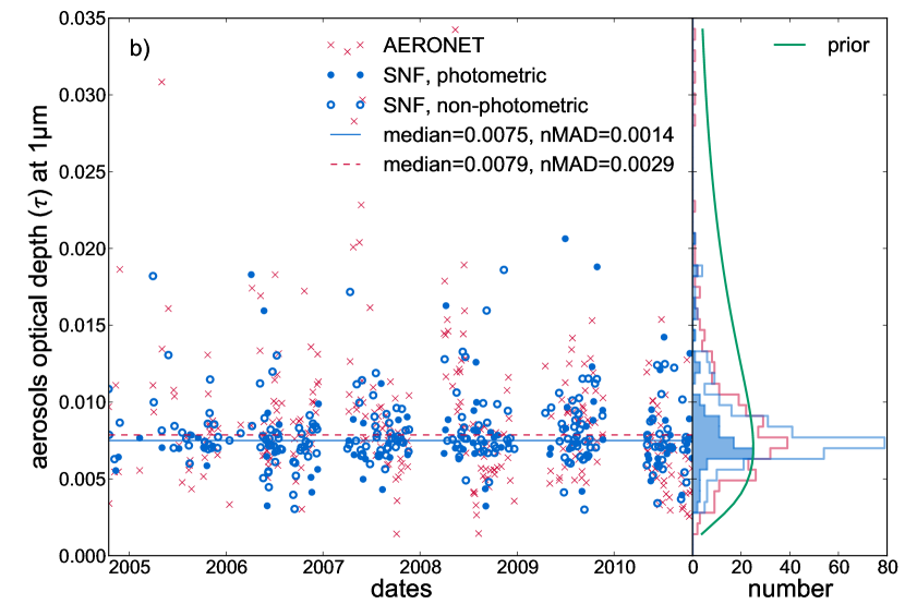
(b)

Figure 19: Aerosol Ångström exponent LABEL:sub@fig:angstrom-exponent and optical depth LABEL:sub@fig:optical-depth distributions from May 2004 to December 2010 for the SNfactory (circles) and the Mauna Loa Observatory (crosses) measurements. Only the common nights of both data sets are presented. Mauna Loa aerosol data were not available for 2011 in time for our analysis.

The SNfactory Ångström exponent, $\aa$, from 2004 to 2011 is distributed between $-2$ and 4. The fact that the Mauna Kea site is almost 1000 m higher than MLO, and the fact that the AERONET observations are carried out during day time make a point to point comparison difficult. Nevertheless, the general features of both distributions still can be compared with each other: the mean SNfactory Ångström exponent ($1.3\pm 1.4$) is compatible with the one measured by AERONET ($1.2\pm 0.9$).

We see in Fig. 19b that the SNfactory aerosol optical depth mean value is slightly smaller than the Mauna Loa mean value (still, they are compatible with each other), and the distribution does not show the slight seasonal trend observed in the AERONET data. Nevertheless, we do expect to have more stable values since the measurements are made at night far above the inversion layer, and the mean optical depth value is compatible with aerosols from maritime origins.

8.3 Telluric absorption comparison

Patat et al. (2011) showed that the water band equivalent width at 7200 Å is well correlated with the Preciptable Water Vapor (PWV) at the Paranal site in Chile. In order to check the consistency of our approach, we compare our water intensity measurement to the PWV amount at Mauna Kea. For that purpose, we used the optical depth at 225 GHz data from the Caltech Submillimeter Observatory (CSO, Peterson et al., 2003) and the empirical formula from Otárola et al. (2010) to compute the PWV at Mauna Kea during the SNfactory observation campaign (cf. Fig. 20). Plotting the computed telluric water intensity (below 9000 Å) with respect to the PWV (cf. Fig. 21), we found that both quantities were highly correlated, reinforcing the findings of Patat et al. (2011) and validating our water telluric correction approach. Furthermore, using an orthogonal distance regression we find a saturation exponent of $\rho=0.62\pm 0.01$ from the best power law describing the distribution (cf. red curve in Fig. 21). This is in excellent agreement with the value $\rho_{\mathrm{H_{2}O}}=0.6$ determined from the airmass dependence of $I_{\mathrm{H_{2}O}}$ in the SNfactory dataset.

Figure 20: Precipitable Water Vapor (PWV) above the Mauna Kea summit during the SNfactory observation campaign. The PWV is empirically computed (Otárola et al., 2010) from the atmospheric optical depth at 225 GHz data by the 225 GHz tipping radiometer at the Caltech Submillimeter Observatory (Peterson et al., 2003).

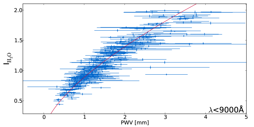
Figure 21: Correlation between the intensity $I_{\mathrm{H_{2}O}}$ of the water telluric line computed from the SNfactory data and the Precipitable Water Vapor gathered from the Caltech Submillimeter Observatory. The red line represents the best power law fit of the distribution with an exponent value of 0.62 — close to the water saturation parameter of 0.6 used in our procedure.

9 Revisiting standard assumptions

A major strength of our analysis comes from the homogeneity and temporal sampling of the SNfactory data set. It consists of a large number of spectro-photometric standard star spectra observed, processed and analyzed in a uniform way. In addition, the sampling candence is frequent and covers a long period of time. Observations were taken under a wide range of atmospheric conditions, including drastically non-photometric nights, which allows us to test many of the standard assumptions used in spectrophotometry, some of which we employed in § 3. In particular, the range of conditions allows us to check our atmospheric model under conditions of strong extinction by clouds, something that has not been done before with spectroscopy simultaneously covering the full ground-based optical window.

9.1 Grey extinction

Using the software package Optical Properties of Aerosols and Clouds (OPAC, Hess et al., 1998), we simulated $\sim 5$ mag of extinction by clouds. While useful observations under such conditions would be unlikely, this large opacity makes it possible to detect any non-grey aspect of cloud extinction. We analyzed three types of cloud (cumulus, stratus and cirrus) in a maritime environment using the standard characteristics from OPAC. The results, as shown in Fig. 22, demonstrate that extinction from cumulus and stratus do exhibit a small trend in wavelength. But even for such strong extinction of 5 mag/airmass the change in transmission from 3200 Å to 10000 Å is below 3%. Cirrus with less than 1 mag of extinction is the most common cloud environment that still allows useful observing, and Fig. 22 demonstrates that such clouds would be grey to much better than 1%.

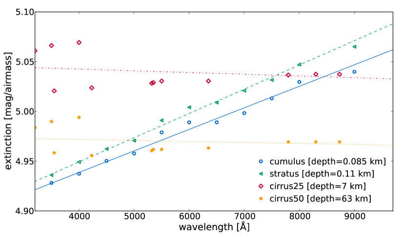
Figure 22: Simulations using OPAC of the wavelength dependence for typical clouds (in maritime environment) through very strong — $\sim 5$ magnitudes — of extinction. Even with such strong extinction, the trend from 3200 Å to 9700 Å is of the order of 3% for cumulus and stratus and negligible for cirrus.

Although atmospheric conditions such as these are usually avoided or inappropriate for observations, we wanted to check whether or not such an effect was visible in our data. Therefore, we gathered 11 observations (cf. Fig. 23) of the standard star GD71 affected by different levels of cloud extinction (from 0.7 to 4.5 mag/airmass). We calibrated these spectra without introducing our grey extinction correction factor, $\delta T$. We then performed a $\chi^{2}$ test that showed that the resulting extinction curves are compatible with a constant to better than 1% across the full wavelength coverage of SNIFS.

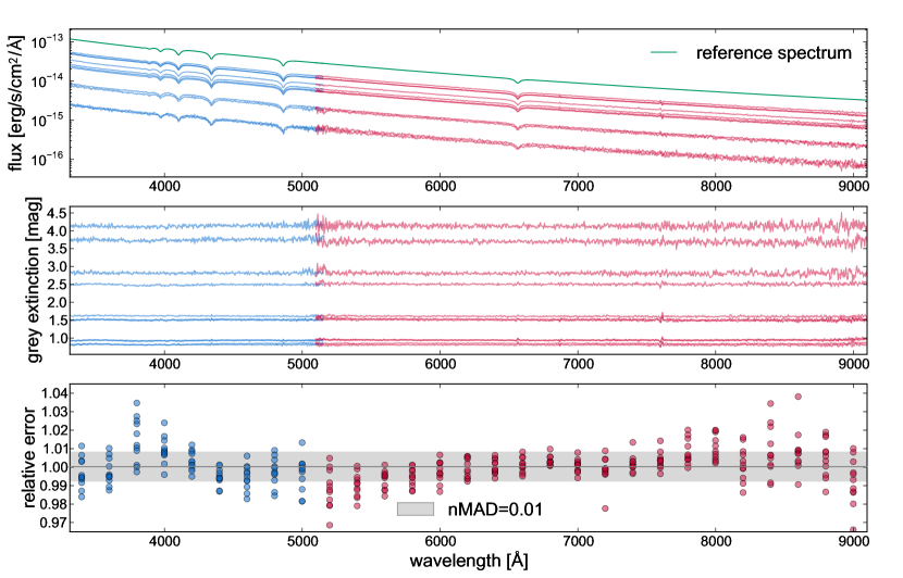
Figure 23: SNfactory observations of the standard star GD71 under various level of cloud extinction during non photometric nights. The top panel shows the flux-calibrated spectra from both spectroscopy channels, without grey extinction correction, compared with the standard star reference template (green). The middle panel shows the additional extinction $\delta T(\lambda,\hat{z},t)$. The bottom panel shows the variation with wavelength of the ratios spectra/reference. It is notable that even with strong extinction by clouds the transmission is compatible with grey extinction ($\delta T(\lambda,\hat{z},t)=\delta T(\hat{z},t)$) at the $\sim 1$% level (grey band).

Our findings using spectroscopy agree with theoretical expectations and the OPAC clouds models. They also agree with the observational analysis by Ivezic et al. (2007) based on repeated broadband filter images of the same Sloan Digital Sky Survey (SDSS) field, which show only a very weak dependence of the photometric residuals with color, even through several magnitudes of extinction by clouds, and even when comparing the flux in the $U$ and $Z$ bands. Similarly Burke et al. (2010) find little sign of color variation from $g-r$, or separately $r-i$, $i-z$ and $z-y$, colors synthesized from their spectroscopic measurements.

As a final check, we can compare the median extinction curves from photometric and non-photometric nights. Fig. 24 shows the difference of these two extinction curves. The agreement is much better than 1% over the full optical window. The smooth trend is due to the aerosol component of our extinction model, and may be a hint either of slight coloring due to clouds or a small difference in the aerosol size distribution with and without clouds. A small residual due to ozone is also apparent.

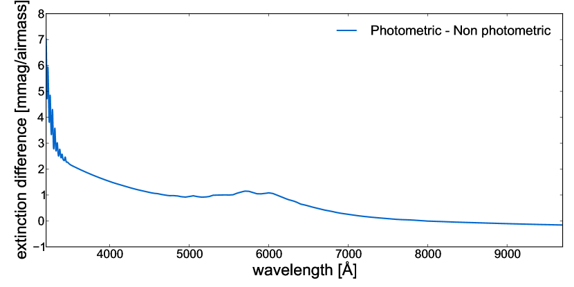
Figure 24: The difference, in [mag/airmass], between the median extinction measured on photometric nights and the median extinction measured on non-photometric nights.

Altogether, we confirm that the treatment of cloud extinction being grey remains valid at the 1% level or better.

9.2 Stability of the instrument

In § 3 we assumed that the instrument calibration, $C(\lambda,t)$, would be stable over the course of a night. Here we provide further justification for this assumption.

To begin, we note that there are several possible sources that could lead to changes in the instrument calibration. Dust accumulation on exposed optics alone can amount to 1 mmag/day per surface, gradually reducing the reflectivity of the telescope mirror and transmission of the spectrograph entrance window. In our case, the telescope tube is closed and the observatory dome is unvented, so dust accumulation on the telescope optics is minimized. The telescope mirrors are regularly cleaned with CO₂ “snow” and realuminized occasionally.

Because the spectrograph optics are enclosed, their transmission is expected to be stable (except for the dichroic beam-splitter which shows changes with humidity — an effect corrected in our pipeline). The quantum efficiency of the detectors will depend on the cold-head temperature at the very reddest wavelengths, where phonons can assist an electron into the conduction band. The electronics could experience drift, though our gain tests using X-rays in the lab and photon transfer curves in situ do not show this.

To experimentally address this issue we have measured the stability of $C(\lambda,t)$ over the course of several nights under photometric conditions. In this test $C(\lambda,t)$ was found to be consistent from one night to another at better than the percent level using the method developed in § 6.2.

In a separate test we compared $C(\lambda,t)$ using 23 standard stars observed throughout the same highly non-photometric night. When divided by their mean, we find that the RMS of the distribution is below the percent level. In this case, because we allow for clouds, only chromatic effects can be tested. Fig. 25 shows the excellent agreement throughout the night.

Of course it is important to keep in mind that major events, such as cleaning or realuminization of the mirror, or instrument repairs, can change the value of $C(\lambda,t)$ significantly. The desire to avoid the need to explicitly account for such events, and the good nightly consistency demonstrated above, justifies our choice to assume that $C(\lambda,t)=C(\lambda)$ during a night, while enabling it to change from one night to another.

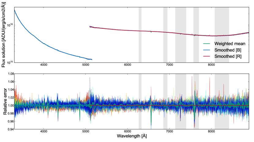
Figure 25: Instrument calibrations, $C(\lambda)$, for 23 observations of GD71 from the same highly non-photometric night (top panel). Relative error of each instrument calibration with respect to the mean value (bottom panel). The mean RMS over the whole wavelength range is $\leavevmode\nobreak\ 0.007$ and the features are due to spectral resolution issues between the spectra and their reference. Poorer accuracy due the water telluric band in the region redward 8900 Å is noticeable.

9.3 Line of sight dependency

One assumption that we have not directly tested is the dependence, or lack thereof, of extinction on the viewing direction. Rayleigh and ozone extinction variations across the sky will be negligible. Aerosols, transported by winds, can be variable and so could vary across the sky. Due to the very low level of aerosols typically encountered over Mauna Kea, detection of such aerosol variations would require an intensive campaign with SNIFS, or better yet, with a LIDAR system. The very low rates of change in aerosol optical depth found in the AERONET data for nearby Mauna Loa (e.g. Stubbs et al., 2007) suggest that variations across the sky will be small or rare. Even for Cerro Tololo, a site at significantly lower altitude and surrounded by dry mountains (the Andes foothills) rather than ocean, Burke et al. (2010) find little evidence for aerosol gradients across the sky. Thus, while we have not been able to directly test the assumption of sightline independence for our extinction measurements, any residual effects are likely to be small. On non-photometric nights the achromatic portion of any sightline dependence would be absorbed into the grey extinction term. In any event, any such spatio-temporal variations will be averaged away across our large dataset.

10 Conclusions

We have derived the first fully spectroscopic extinction curve for Mauna Kea that spans the entire optical window and samples hundreds of nights. The median parameters, tabulated in Table 4, and the median curve, tabulated in Table 6, can be used to correct past and future Mauna Kea data for atmospheric extinction. Comparison of our median extinction curve shows good agreement in regions of overlap with previously published measurements of Mauna Kea atmospheric extinction (Boulade, 1987; Krisciunas et al., 1987; Bèland et al., 1988) even though the measurements are separated by roughly 20 years.

Our large dataset of 4285 spectra of standard stars collected over 7 years means that a wide range of conditions has been sampled. Using this, we estimate the per-night variations on the extinction curve (see Table 6), and this can be employed by others to estimate the uncertainty in their data when using the median extinction curve rather than deriving their own nightly flux calibration. This is especially important for Mauna Kea due to the presence of several of the world’s largest telescopes, for which time spent on calibration is often at odds with obtaining deeper observations, and where calibration to a few percent is often deemed adequate by necessity.

The method providing the extinction we have introduced in this paper has several notable features. First, it borrows techniques long used in the atmospheric sciences to decompose the extinction into its physical components. This allows robust interpolation over wavelengths affected by features in the spectra of the standard stars, and it accounts for even weak extinction correlations spanning across wavelengths that would otherwise be hard to detect. We have also utilized a method of dealing with clouds by which the non-cloud component of the extinction still can be measured. This enables chromatic flux calibration even through clouds, and with an external estimate of the cloud component alone (such as through the SNIFS Multi-filter ratios) allows accurate flux calibration even in non-photometric conditions.

Because of these desirable properties, we encourage the broader use of this technique for flux calibration in astronomy. Furthermore, we note that this parametric template is especially easy to use for simulating the flux calibration requirements for future surveys (The atmospheric extinction computation code is available from the SNfactory software web site http://snfactory.in2p3.fr/soft/atmosphericExtinction/).

Finally, we have used our large homogeneous dataset to examine several standard assumptions commonly made in astronomical flux calibration, like the greyness of the clouds, and we confirmed our instrument stability. These assumptions are usually difficult for most astronomers to verify with their own data, which usually spans just a few nights. We draw attention to the fact that the altitude of Mauna Kea and the generally strong inversion layer sitting well below the summit helps minimize the impact of aerosols and water vapor. These features are often neglected relative to metrics related to image quality, but they help make Mauna Kea an excellent site also for experiments requiring accurate flux calibration.

Table 4: Summary of the median values for the various adjusted physical quantities. For $\delta T$ which represents the cloud extinction, the absolute scale mean value is meaningless (as explained in 6.2.1), only variability could have an interest as an estimate of grey fluctuations during non-photometric conditions.

Parameter	Median $\pm$	nMAD	Description
$\delta T$	1.04 $\pm$	0.34	grey extinction (mean & RMS)
$I_{\mathrm{O_{3}}}$	257.4 $\pm$	23.3	$\mathrm{O_{3}}$ intensity
$\tau$	0.0084 $\pm$	0.0014	aerosol optical depth
$\aa$	1.26 $\pm$	1.33	aerosol Ångström exponent
$\rho_{\mathrm{O_{2}}}$	0.58 $\pm$	0.04	telluric $\mathrm{O_{2}}$ saturation
$\rho_{\mathrm{H_{2}O}}$	0.60 $\pm$	0.27	telluric $\mathrm{H_{2}O}$ saturation

Table 5: List of the standard stars used in SNfactory for flux calibration purposes (i.e. computation of the nightly atmospheric extinction, the nightly telluric correction template and the instrument calibration).

Standard Star	Number of	R.A (J2000)	Dec. (J2000)	Magnitude ($V$)	Type
	Observations
BD+174708	237	22 11 31.37	+18 05 34.2	9.91	sdF8
BD+254655	90	21 59 42.02	+26 25 58.1	9.76	O
BD+284211	92	21 51 11.07	+28 51 51.8	10.51	Op
BD+332642	66	15 51 59.86	+32 56 54.8	10.81	B2IV
BD+75325	75	08 10 49.31	+74 57 57.5	9.54	O5p
CD-32d9927	21	14 11 46.37	-33 03 14.3	10.42	A0
EG131	270	19 20 35.00	-07 40 00.1	12.3	DA
Feige110	145	23 19 58.39	-05 09 55.8	11.82	DOp
Feige34	128	10 39 36.71	+43 06 10.1	11.18	DO
Feige56	36	12 06 42.23	+11 40 12.6	11.06	B5p
Feige66	44	12 37 23.55	+25 04 00.3	10.50	sdO
Feige67	32	12 41 51.83	+17 31 20.5	11.81	sdO
G191B2B	102	05 05 30.62	+52 49 54.0	11.78	DA1
GD153	209	12 57 02.37	+22 01 56.0	13.35	DA1
GD71	165	05 52 27.51	+15 53 16.6	13.03	DA1
HD93521	227	10 48 23.51	+37 34 12.8	7.04	O9Vp
HR1544	226	04 50 36.69	+08 54 00.7	4.36	A1V
HR3454	159	08 43 13.46	+03 23 55.1	4.30	B3V
HR4468	127	11 36 40.91	-09 48 08.2	4.70	B9.5V
HR4963	164	13 09 56.96	-05 32 20.5	4.38	A1IV
HR5501	202	14 45 30.25	+00 43 02.7	5.68	B9.5V
HR718	253	02 28 09.54	+08 27 36.2	4.28	B9III
HR7596	325	19 54 44.80	+00 16 24.6	5.62	A0III
HR7950	236	20 47 40.55	-09 29 44.7	3.78	A1V
HR8634	255	22 41 27.64	+10 49 53.2	3.40	B8V
HR9087	210	00 01 49.42	-03 01 39.0	5.12	B7III
HZ21	63	12 13 56.42	+32 56 30.8	14.68	DO2
HZ44	30	13 23 35.37	+36 08 00.0	11.66	sdO
LTT1020	45	01 54 49.68	-27 28 29.7	11.52	G
LTT1788	26	03 48 22.17	-39 08 33.6	13.16	F
LTT2415	57	05 56 24.30	-27 51 28.8	12.21	sdG
LTT377	41	00 41 46.82	-33 39 08.2	11.23	F
LTT3864	12	10 32 13.90	-35 37 42.4	12.17	F
LTT6248	32	15 39 00.02	-28 35 33.1	11.80	A
LTT9239	36	22 52 40.88	-20 35 26.3	12.07	F
LTT9491	56	23 19 34.98	-17 05 29.8	14.11	DC
NGC7293	39	22 29 38.46	-20 50 13.3	13.51	V.Hot
P041C	31	14 51 58.19	+71 43 17.3	12.00	GV
P177D	119	15 59 13.59	+47 36 41.8	13.47	GV

Table 6: SNfactory median atmospheric extinction [mag/airmass], its variability (RMS and nMAD of all the individual extinctions) and its decomposition into physical components from 3200 Å to 10000 Å (100 Å bins). A complete table with a 2 Å binning is available in electronic form at the CDS via anonymous ftp to cdsarc.u-strasbg.fr (130.79.128.5) or via http://cdsweb.u-strasbg.fr/cgi-bin/qcat?J/A+A/.

Wavelength [Å]	Total Extinction	Variability		Rayleigh	Ozone	Aerosols
		RMS	nMAD
3200	0.856	-	-	0.606	0.214	0.036
3300	0.588	0.057	0.041	0.532	0.021	0.035
3400	0.514	0.053	0.040	0.469	0.012	0.033
3500	0.448	0.048	0.039	0.415	0.001	0.032
3600	0.400	0.045	0.037	0.369	0.000	0.031
3700	0.359	0.042	0.035	0.329	0.000	0.030
3800	0.323	0.039	0.034	0.294	0.000	0.029
3900	0.292	0.036	0.032	0.264	0.000	0.028
4000	0.265	0.033	0.030	0.238	0.000	0.027
4100	0.241	0.031	0.029	0.215	0.000	0.026
4200	0.220	0.029	0.027	0.194	0.000	0.026
4300	0.202	0.027	0.026	0.176	0.001	0.025
4400	0.185	0.026	0.025	0.160	0.001	0.024
4500	0.171	0.024	0.023	0.146	0.001	0.023
4600	0.159	0.023	0.022	0.134	0.003	0.023
4700	0.147	0.021	0.021	0.122	0.003	0.022
4800	0.139	0.020	0.020	0.112	0.005	0.022
4900	0.130	0.019	0.019	0.103	0.006	0.021
5000	0.125	0.018	0.017	0.095	0.009	0.021
5100	0.119	0.017	0.016	0.087	0.012	0.020
5200	0.114	0.016	0.015	0.081	0.013	0.020
5300	0.113	0.015	0.014	0.075	0.019	0.019
5400	0.109	0.015	0.013	0.069	0.022	0.019
5500	0.106	0.014	0.013	0.064	0.024	0.018
5600	0.107	0.013	0.012	0.060	0.029	0.018
5700	0.108	0.013	0.012	0.056	0.035	0.017
5800	0.103	0.012	0.011	0.052	0.034	0.017
5900	0.098	0.012	0.011	0.048	0.033	0.017
6000	0.098	0.011	0.010	0.045	0.037	0.016
6100	0.092	0.011	0.010	0.042	0.034	0.016
6200	0.084	0.010	0.009	0.039	0.029	0.016
6300	0.078	0.010	0.009	0.037	0.026	0.015
6400	0.070	0.009	0.008	0.035	0.021	0.015
6500	0.065	0.009	0.008	0.033	0.018	0.015
6600	0.060	0.008	0.007	0.031	0.015	0.014
6700	0.056	0.008	0.007	0.029	0.013	0.014
6800	0.052	0.008	0.007	0.027	0.011	0.014
6900	0.048	0.007	0.006	0.026	0.008	0.014
7000	0.044	0.007	0.006	0.024	0.007	0.013
7100	0.042	0.007	0.006	0.023	0.006	0.013
7200	0.039	0.006	0.005	0.022	0.005	0.013
7300	0.037	0.006	0.005	0.020	0.004	0.013
7400	0.035	0.006	0.005	0.019	0.003	0.013
7500	0.033	0.006	0.004	0.018	0.003	0.012
7600	0.032	0.005	0.004	0.017	0.002	0.012
7700	0.030	0.005	0.004	0.016	0.002	0.012
7800	0.029	0.005	0.004	0.016	0.002	0.012
7900	0.028	0.005	0.004	0.015	0.002	0.012
8000	0.027	0.005	0.003	0.014	0.001	0.011
8100	0.026	0.004	0.003	0.013	0.001	0.011
8200	0.025	0.004	0.003	0.013	0.001	0.011
8300	0.024	0.004	0.003	0.012	0.001	0.011
8400	0.023	0.004	0.003	0.012	0.001	0.011
8500	0.023	0.004	0.002	0.011	0.001	0.011
8600	0.022	0.004	0.002	0.011	0.001	0.010
8700	0.021	0.004	0.002	0.010	0.001	0.010
8800	0.021	0.004	0.002	0.010	0.001	0.010
8900	0.020	0.003	0.002	0.009	0.001	0.010
9000	0.019	0.003	0.002	0.009	0.001	0.010
9100	0.019	0.003	0.002	0.008	0.001	0.010
9200	0.018	0.003	0.002	0.008	0.001	0.010
9300	0.018	0.003	0.002	0.008	0.001	0.009
9400	0.017	0.003	0.001	0.007	0.001	0.009
9500	0.017	0.003	0.001	0.007	0.000	0.009
9600	0.016	0.003	0.001	0.007	0.000	0.009
9700	0.016	0.003	0.001	0.006	0.000	0.009
9800	0.015	-	-	0.006	0.000	0.009
9900	0.015	-	-	0.006	0.000	0.009
10000	0.014	-	-	0.006	0.000	0.009