IIB Duals of $D=3$ ${\cal N}=4$ Circular Quivers

Abstract

We construct the type-IIB $AdS_{4}\ltimes K$ supergravity solutions which are dual to the three-dimensional ${\cal N}=4$ superconformal field theories that arise as infrared fixed points of circular-quiver gauge theories. These superconformal field theories are labeled by a triple $(\rho,\hat{\rho},L)$ subject to constraints, where $\rho$ and $\hat{\rho}$ are two partitions of the same number $N$, and $L$ is a positive integer. We show that in the limit of large $L$ the localized five-branes in our solutions are effectively smeared, and these type-IIB solutions are dual to the near-horizon geometry of M-theory M2-branes at a $\mathbb{C}^{4}/(Z_{k}\times Z_{\hat{k}})$ orbifold singularity. Our IIB solutions resolve the singularity into localized five-brane throats, without breaking the conformal symmetry. The constraints satisfied by the triple $(\rho,\hat{\rho},L)$, together with the enhanced non-abelian flavour symmetries of the superconformal field theories, are precisely reproduced by the supergravity solutions. As a bonus, we uncover a novel type of “orbifold equivalence” between different quantum field theories and provide quantitative evidence for this equivalence.

LPTENS-12/34

Imperial/TP/2012/JE/02

^♮ Laboratoire de Physique Théorique de l’École Normale Supérieure,

24 rue Lhomond, 75231 Paris cedex, France

^∗ Blackett Laboratory, Imperial College,

London, SW7 2AZ, United Kingdom

^♭ Instituut voor Theoretische Fysica, KULeuven,

Celestijnenlaan 200D B-3001 Leuven, Belgium

^† Perimeter Institute for Theoretical Physics,

Waterloo, Ontario, N2L2Y5, Canada

¹benjamin.assel@lpt.ens.fr, ²bachas@lpt.ens.fr,

³johnaldonestes@gmail.com, ⁴jgomis@perimeterinstitute.ca

1 Introduction

Conformal field theories play a distinguished role in the space of all quantum field theories. They reside at fixed points of the renormalization group, which generates a flow in the space of quantum field theories. Any non-conformal field theory can be reached under renormalization group evolution by perturbing a conformal theory with a suitable operator. The central role that conformal field theories play in our understanding of quantum field theory is one of the reasons why they have been a subject of enduring interest.

A large class of conformal field theories can be obtained by perturbing a Gaussian fixed-point theory in the ultraviolet by a relevant operator, and following the renormalization group flow in the infrared. Infrared fixed points which arise after “long” renormalization group flows are, however, inherently strongly coupled, and therefore not amenable to study with conventional field theory techniques. The discovery of the AdS/CFT correspondence [1, 2, 3] has opened a new window into the world of strongly-coupled conformal field theories, turning the study of some of them (in the large $N$ limit) to the study of string theory in asymptotically anti-de-Sitter backgrounds.

In this paper, we provide the type-IIB string theory backgrounds dual to a very large class of strongly coupled, three dimensional ${\cal N}=4$ superconformal field theories. These backgrounds have a warped $AdS_{4}\ltimes K$ geometry with very specific five-brane sources. They are dual to the non-trivial infrared fixed points of three-dimensional ${\cal N}=4$ supersymmetric gauge theories corresponding to circular quiver gauge theories depicted in figure 2. These quiver gauge theories admit an elegant realization in terms of the low energy limit of intersecting brane configurations [4]. The dual type-IIB backgrounds we construct encode the backreacted near-horizon geometry of these brane configurations.

The circular quiver gauge theories that give rise to irreducible superconformal field theories in the infrared are labeled by the triple

$$(\rho,\hat{\rho},L)\,,$$

where $\rho$ and $\hat{\rho}$ are two ordered partitions of $N$ and $L$ is a positive integer. In order for the ultraviolet quiver gauge theory to be well defined, the Young tableaux corresponding to the partitions $\rho$ and $\hat{\rho}$ must satisfy a set of constraints which can be summarized, as we will explain, by the inequality

$$\rho^{T}+L>\hat{\rho}\,.$$ (1.1)

Besides being invariant under the $OSp(4|4)$ superconformal symmetry group, these infrared fixed-point theories have a rich pattern of global symmetries that go beyond those present in the theory in the ultraviolet. For a superconformal field theory emerging from a circular quiver labeled by partitions $\rho$ and $\hat{\rho}$, the infrared theory acquires an enhanced global symmetry

$$H_{\rho}\times H_{\hat{\rho}}\,,$$ (1.2)

where $H_{\sigma}$ is the commutant of $SU(2)$ in $U(N)$ for the embedding $\sigma:SU(2)\rightarrow U(N)$ characterized by the partition $\sigma$ of $N$. The explicit $AdS_{4}\ltimes K$ type-IIB string backgrounds we construct provide a concrete realization of the constraints (1.1) and reproduce the precise pattern of global symmetries (1.2).

The construction of these string backgrounds extends previous work in [5, 6], where the bulk description of the strongly coupled, three dimensional ${\cal N}=4$ superconformal field theories that arise as infrared fixed points of linear quiver gauge theories was presented. All these solutions emerge from the analysis of the equations derived in [7] (see also [8]) which determine the most general $OSp(4|4)$ invariant type-IIB supergravity backgrounds. These equations can be, in turn, elegantly solved [9, 10] in terms of two harmonic functions on an open Riemann surface. The Riemann surface relevant for the linear quivers is a strip, whereas the one relevant for circular quivers is an annulus. Pleasingly, the data of a circular quiver gauge theory which flows to a superconformal field theory in the infrared is encoded in special “punctures” at the boundary of the annulus.

A class of three-dimensional ${\cal N}=4$ superconformal field theories that arise from circular quivers are known to admit an M-theory description in terms of orbifolds of the seven-sphere [11, 12, 13]. By taking a certain (large $L$) smearing limit of our solutions, T-dualizing the periodic coordinate of the annulus and lifting the resulting type-IIA background to eleven dimensions, we reproduce the relevant M-theory geometries ${\rm AdS}_{4}\times{\rm S}^{7}/(\mathbb{Z}_{k}\times\mathbb{Z}_{\hat{k}})$. In the process one looses however the dependence on the full quiver data $(\rho,\hat{\rho},L)$. This data can be in principle encoded in the non-contractible 3-cycles of the compact space and the associated 3-form fluxes [13, 14, 15, 16]. The 3-cycles degenerate however in the orbifold limit, and we are not aware of any solutions of eleven-dimensional supergravity that resolve the singularity on the M-theory side. By contrast in our IIB solutions, the full data is encoded in the positions of five-brane throats along the annulus circle, and the singularity is effectively resolved.

An interesting outcome of our investigations is a new type of “orbifold equivalence” between different quantum field theories. Based on the $SL(2,\mathbb{R})$ symmetry of type-IIB supergravity we arrive at the conjecture that gauge theories living on brane configurations which are related by $SL(2,\mathbb{Q})$ transformations are equivalent in a certain large $N$ limit. Theories related by $SL(2,\mathbb{Z})$ transformations are of course exactly equivalent, or mirror-symmetric, while more general $SL(2,\mathbb{Q})$ transformations can be regarded as orbifoldings of the F-theory torus. A similar generalization of the T-duality group $O(d,d,\mathbb{Z})$ to a semigroup extension of $O(d,d,\mathbb{Q})$ has been analyzed recently in [21]. We provide quantitative evidence for this new orbifold equivalence by explicitly computing the partition function on $S^{3}$ of two different theories, which are related by $SL(2,\mathbb{Q})$, and showing that these partition functions match exactly.

The plan of the rest of the paper is as follows. In section 2 we introduce the linear and circular quivers, which are the main objects of study in this paper. We also recall the conditions under which an ultraviolet quiver gauge theory is expected to flow in the infrared to an irreducible superconformal field theory and provide the data and constraints characterizing irreducible superconformal field theories, both for linear and circular quivers. In section 3 we present the supergravity solutions corresponding to the fixed points arising from circular quivers, also introducing the main features of the solutions corresponding to linear quivers that are needed for our analysis. In section 4 we establish the dictionary between the infrared SCFTs and our supergravity solutions and find perfect agreement. Section 5 contains the analysis of various interesting limits of the solutions and discusses their interpretation. This includes an interesting “smeared” limit that results in M-theory geometries describing M2-branes at orbifold singularities. In section 6 we explain how our supergravity solutions can be used to yield theories that are equivalent under a novel type of “orbifold equivalence”. We provide quantitative evidence for this by computing the large $N$ partition function of a proposed dual pair and we find perfect agreement. We have relegated to the Appendices some details and computations.

2 Quivers, Infrared Fixed Points and Branes

2.1 Linear and circular quivers

The three-dimensional ${\cal N}=4$ superconformal field theories considered in this paper arise as non-trivial infrared fixed points of three-dimensional quiver gauge theories with ${\cal N}=4$ supersymmetries. Their field content and their microscopic Lagrangians are succinctly summarized by a quiver diagram [22]. In our case the diagrams will have either linear or circular topology (see figures 1 and 2). We refer to the corresponding quivers as linear and circular respectively.

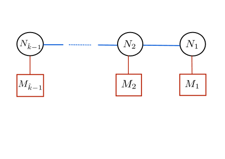
Figure 1: A linear quiver with $\hat{k}-1$ gauge-group factors $U(N_{1})\times U(N_{2})\times\cdots$. The red boxes indicate the numbers of hypermultiplets in the fundamental representation of each gauge-group factor.

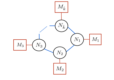
Figure 2: A circular quiver with $\hat{k}$ gauge-group factors. The $U(N_{i})$ theories interact via bifundamental hypermultiplets (the blue lines) which form a circular chain, as opposed to the linear chain of figure 1.

The vector multiplets of these quiver gauge-field theories transform in the adjoint representation of the gauge group

$$U(N_{1})\times U(N_{2})\times...\ U(N_{i})\times...\,.$$ (2.1)

Moreover, these theories contain a hypermultiplet transforming in the bifundamental representation of each consecutive pair of gauge groups $U(N_{i})\times U(N_{i+1})$. For linear quivers $1\leq i\leq\hat{k}-2$, while for the circular quivers $1\leq i\leq\hat{k}$ with the convention that $U(N_{\hat{k}+1})\equiv U(N_{1})$. Finally, there are $M_{i}$ hypermultiplets in the fundamental representation of the group $U(N_{i})$.

A central question about the dynamics of these gauge theories is whether they flow to a non-trivial fixed point of the renormalization group in the infrared. Since massive fields decouple in the infrared, we will assume that hypermultiplet masses and Fayet-Iliopoulos terms are set to zero. We also assume for now vanishing Chern-Simons terms – we will consider however such terms later in the paper. The quiver data and the extended ${\cal N}=4$ supersymmetry specify then completely the microscopic, renormalizable Lagrangian.

We are interested in “irreducible superconformal field theories”, i.e. theories not containing a decoupled sector with free vector multiplets and/or free hypermultiplets. It has been conjectured by Gaiotto and Witten [23] that a necessary and sufficient condition for a gauge theory to flow to an irreducible superconformal field theory is

$$N_{F,i}\geq 2N_{i}\,.$$ (2.2)

In words, each gauge-group factor $U(N_{i})$ should have at least $2N_{i}$ hypermultiplets transforming in the fundamental representation. A more refined irreducibility condition will be discussed below. Recall that a hypermultiplet in the fundamental and anti-fundamental representation are equivalent. Therefore, for a quiver gauge theory, the above requirement of irreducibility in the infrared imposes the following inequalities on the quiver data

$$M_{i}+N_{i-1}+N_{i+1}\geq 2N_{i}\,.$$ (2.3)

One way to argue for the above conditions is that when they are obeyed the gauge group can be completely Higgsed [24], and there exists a singularity at the origin of the Higgs branch, from which the Coulomb branch emanates. A non-trivial superconformal field theory appears in the infrared limit of the gauge theory around that vacuum. Conversely, when complete Higgsing is not possible, decoupled multiplets remain in the infrared, thus yielding non-irreducible theories.

The quiver data that characterizes the irreducible superconformal field theories can be repackaged in a convenient way in terms of two partitions, $\rho$ and $\hat{\rho}$, of the same number N (this is explained below). As usual, one can associate a Young tableau to each partition. The quiver theory can be described by the following data

$\bullet\$ for linear quivers : $(\rho,\hat{\rho})$ subject to the constraints

$$\rho^{T}>\hat{\rho}\ ;$$ (2.4)

$\bullet\$ for circular quivers: $(\rho,\hat{\rho},L)$ subject to the constraints

$$\rho^{T}\geq\hat{\rho}\ ,\qquad L>0\,.$$ (2.5)

Here $\rho$ and $\hat{\rho}$ denote the two partitions of $N$, and $L$ is a positive integer. The inequality $\rho>\sigma$ between partitions means that the total number of boxes in the first $n$ rows of $\rho$ exceeds the same number in $\sigma$, for all $n$. Transposition interchanges the columns and rows of a Young tableau. The inequality (2.4) has appeared previously in different contexts related to solutions of Nahm’s equations, see e.g. [25, 26].

We denote the linear-quiver theory associated to $(\rho,\hat{\rho})$ by $T_{\hat{\rho}}^{\rho}(SU(N))$, and the circular-quiver theory with data $(\rho,\hat{\rho},L)$ by $C_{\hat{\rho}}^{\rho}(SU(N),L)$. It turns out that the above Young-tableaux constraints are automatically satisfied if the ranks of all the gauge groups of the ultraviolet theories are positive, that is if all $N_{i}>0$. If some Young-tableaux inequalities were saturated for a linear quiver, the quiver would break down to decoupled quivers plus free hypermultiplets. Circular quivers, on the other hand, degenerate to linear quivers when $L=0$.

As we shall see, this data also completely encodes the field content of the ultraviolet mirror pair [27] of quiver gauge theories which flow to the same fixed point in the infrared. Mirror symmetry for this class of quiver gauge theories is realized very simply by the exchange of the two partitions

$$\text{mirror symmetry}:\qquad\rho\longleftrightarrow\hat{\rho}\,.$$ (2.6)

Therefore, $T_{\hat{\rho}}^{\rho}(SU(N))$ and $T_{\rho}^{\hat{\rho}}(SU(N))$ are mirror linear-quiver gauge theories, while $C_{\hat{\rho}}^{\rho}(SU(N),L)$ and $C_{\rho}^{\hat{\rho}}(SU(N),L)$ are mirror circular quivers. The Young tableaux constraints are symmetric under the exchange of $\rho$ and $\hat{\rho}$, see appendix A, and are therefore consistent with mirror symmetry.

These infrared superconformal field theories are believed to have a rich pattern of global symmetries, inherited from the symmetries acting on the Higgs and Coulomb branch of the quiver gauge theory from which the fixed point is reached in the infrared. Since mirror symmetry exchanges the Higgs and Coulomb branches of mirror pairs, we conclude that the global symmetry at the fixed point is

$$H\times\hat{H}\,,$$ (2.7)

where

$$H=\prod_{i}U(M_{i})\qquad{\rm and}\qquad\hat{H}=\prod_{i}U(\hat{M}_{i})\,.$$ (2.8)

$H$ is the symmetry that rotates the fundamental hypermultiplets of $T^{\rho}_{\hat{\rho}}(SU(N))$ or $C_{\hat{\rho}}^{\rho}(SU(N),L)$, while $\hat{H}$ rotates the fundamental hypermultiplets of their mirror duals. The two symmetries coexist at the superconformal fixed point.

In this paper we find the bulk gravitational description of the irreducible three dimensional ${\cal N}=4$ superconformal theories to which circular quiver gauge theories of the above type flow in the infrared. We already presented the supergravity description of the superconformal theories associated to linear quivers in [5].

2.2 Brane Realization

The above three-dimensional ${\cal N}=4$ supersymmetric linear and circular quiver gauge theories admit an elegant realization as the low-energy limit of brane configurations in type-IIB string theory [4]. The brane configuration consists of an array of D3, D5 and NS5 branes oriented as shown in the table.

	0	1	2	3	4	5	6	7	8	9
D3	X	X	X	X
D5	X	X	X		X	X	X
NS5	X	X	X					X	X	X

Table 1: Brane array for three-dimensional quiver gauge theories

For linear quivers, the D3 branes span a finite interval along the $x^{3}$ direction and terminate on the five-branes, while for circular quivers $x^{3}$ parametrizes a circle.

Linear Quivers

The brane configuration corresponding to the linear quiver gauge theory of Figure 1 is depicted in Figure 3. An invariant way of encoding a brane configuration – and the corresponding quiver gauge theory – is by specifying the linking numbers of the five-branes. They can be defined as follows

$$\ l_{i} =-n_{i}+R_{i}^{\rm NS5}\qquad(i=1,...,k)$$ (2.9)

$$\hat{l}_{j} =\hat{n}_{j}+L_{j}^{\rm D5}\qquad(j=1,...,\hat{k})\ ,$$ (2.10)

where $n_{i}$ is the number of D3 branes ending on the $i$th D5 brane from the right minus the number ending from the left, $\hat{n}_{j}$ is the same quantity for the $j$th NS5 brane, $R_{i}^{\rm NS5}$ is the number of NS5 branes lying to the right of the $i$th D5 brane and $L_{j}^{\rm D5}$ is the number of D5 branes lying to the left of the $j$th NS5 brane. These numbers are invariant under Hanany-Witten moves [4], when a D5 brane crosses a NS5 brane. Since the extreme infrared limit is expected to be insensitive to these moves, it is convenient to label the infrared dynamics in terms of the linking numbers.

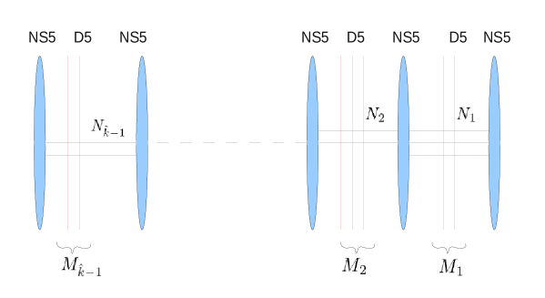
Figure 3: Brane realization of linear quivers

The brane construction of the linear quivers shown in Figure 3 is characterized by the following linking numbers

$$l_{i} = j\quad\textrm{for a D5 brane between the $j$-th and $(j+1)$-th NS5 brane,}$$

$$\textrm{with a labeling such that $l_{1}\geq..\geq l_{k}$};$$

$$\hat{l}_{j} = N_{j-1}-N_{j}+\sum_{s=j}^{\hat{k}-1}M_{s}\quad\textrm{for}\quad j=1,..,\hat{k}.\quad(N_{0}=N_{\hat{k}}=0)\,.$$ (2.12)

We may move all the NS5 branes to the left and all the D5 branes to the right, noting that a new D3 brane is created every time that a D5 crosses a NS5. In the end, all the D3 branes will be suspended between a NS5 brane on the left and a D5 brane on the right, so that the linking numbers satisfy the sum rule

$$\sum_{i=1}^{k}l_{i}=\sum_{j=1}^{\hat{k}}\hat{l}_{j}\equiv N\,,$$ (2.13)

where $N$ is the total number of suspended D3 branes. This implies that the two sets of five-brane linking numbers define two partitions of $N$

$$\rho:\qquad~{}N = l_{1}+\ldots+l_{k}$$ (2.14)

$$= \underbrace{1+\ldots+1}_{M_{1}}\,+\,\underbrace{2+\ldots+2}_{M_{2}}\,+\,\ldots+\ldots$$

$$\hat{\rho}:\qquad~{}N = \hat{l}_{1}+\ldots+\hat{l}_{\hat{k}}$$ (2.15)

$$= \underbrace{1+\ldots+1}_{\hat{M}_{1}}\,+\,\underbrace{2+\ldots+2}_{\hat{M}_{2}}\,+\,\ldots+\ldots\,.$$

This is the repackaging of the quiver data in terms of partitions of $N$, mentioned above. It is illustrated by Figure 4.

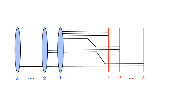
Figure 4: Pushing all D5-branes to the right of all NS5-branes makes it easy to read the linking numbers, as the net number of D3-branes ending on each five-brane. In this example $\rho=(3,2,\cdots 2)$ and $\hat{\rho}=(4,2,\cdots 1)$.

In the original configuration of Figure 3 the D5 brane linking numbers are, by construction, positive and non-increasing, i.e. $l_{1}\geq\cdots\geq l_{i}\geq l_{i+1}\cdots\geq l_{k}>0$, but this is not automatic for the linking numbers of the NS5 branes. Requiring that the NS5 brane linking numbers be non-increasing, that is $\hat{l}_{1}\geq\cdots\geq\hat{l}_{i}\geq\hat{l}_{i+1}\cdots\geq\hat{l}_{\hat{k}}=N_{\hat{k}-1}$, is equivalent, as follows from (2.12), to

$$M_{i}+N_{i-1}+N_{i+1}\geq 2N_{i}\,.$$ (2.16)

This is the same as (2.3), the necessary and sufficient conditions for the corresponding (‘good’) quiver gauge theories to flow to an irreducible superconformal field theory in the infrared. Notice that if these conditions are not obeyed the linking numbers of the NS5 branes need not even be positive integers. Furthermore, for the good theories that obey (2.16), it follows from the expressions (2.12) that the Young tableaux conditions $\rho^{T}>\hat{\rho}$ are automatically satisfied, as long as the rank of each gauge-group factor in the quiver diagram is positive.

In the configuration of Figure 4 on the other hand, the meaning of the above conditions changes. The ordering and positivity of all linking numbers is now automatic (more precisely, it can be trivially arranged by moving 5-branes of the same type past each other). The constraints $\rho^{T}>\hat{\rho}$ on the other hand are non-trivial; they are the ones that guarantee that a supersymmetric configuration like the one of Figure 3 can be reached by a sequence of Hanany-Witten moves [5]. The two types of configuration shown in the figures are in one-to-one correspondence when all these inequalities are satisfied by the five-brane linking numbers.

Summarizing, the linear-quiver ${\cal N}=4$ gauge theories conjectured in [23] to flow to irreducible fixed points in the infrared, without extra free decoupled multiplets, are labeled in an invariant way by two ordered partitions of $N$, with associated Young tableaux $\rho$ and $\hat{\rho}$ subject to the conditions $\rho^{T}>\hat{\rho}$.

Circular Quivers

The brane configuration corresponding to the circular-quiver gauge theory of Figure 2 is given in Figure 5. In this case the $x^{3}$ coordinate along the D3 branes is periodic. Compared to the linear case, there are $N_{\hat{k}}>0$ additional D3 branes extended between the first and the $\hat{k}$th NS5 branes that close the circle. There can be, as well, $M_{\hat{k}}\geq 0$ extra D5 branes giving rise to fundamental hypermultiplets.

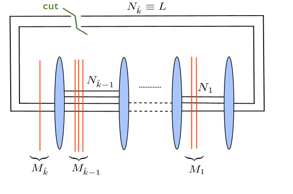
Figure 5: Brane realization of circular quivers. To attribute linking numbers to the five-branes we cut open the $k$-th stack of D3 branes, and place the $k$-th D5 stack at the left-most end.

We can associate linking numbers to the five-branes by cutting open the circular quiver along one of the suspended D3-brane stacks, say the $k$-th stack. We also choose to place the $\hat{k}$-th stack of D5 branes at the left-most end of the open chain, as shown in Figure 5. The linking numbers are gauge-variant quantities, and the above choices amount to fixing partially a gauge. In this gauge the linking numbers read:

$$l_{i} = j\quad\textrm{for the $j$-th stack of D5 branes}\,,$$ (2.17)

$$\hat{l}_{j} = N_{j-1}-N_{j}+\sum_{s=j}^{\hat{k}}M_{s}\ ,\quad\textrm{with}\quad j=1,..,\hat{k}\ .\quad(N_{0}=N_{\hat{k}})$$ (2.18)

As in the case of linear quivers, we label the NS5 branes in order of appearance from right to left, and the D5 branes from left to right.

Defined as above, the linking numbers obey the sum rule (2.13) with $N\equiv\sum_{s=1}^{\hat{k}}sM_{s}$. Furthermore the linking numbers of the D5 branes are by construction non-increasing, positive and bounded by the number of NS5 branes, i.e.

$$\hat{k}\geq l_{1}\geq\cdots l_{i}\geq l_{i+1}\cdots\geq l_{k}>0\ .$$ (2.19)

What about the linking numbers of NS5 branes? For linear quivers, imposing that the $\hat{l}_{j}$ be non-increasing was equivalent to the Higgsing conditions (2.2) that singled out the ‘good theories’, i.e. those believed to flow to an irreducible superconformal fixed point in the infrared. Now, the Higgsing conditions can be written as

$$0 \leq N_{j+1}+N_{j-1}-2N_{j}+M_{j}=\hat{l}_{j}-\hat{l}_{j+1}\quad\textrm{for}\,\ j=1,..,\hat{k}-1$$ (2.20)

$$0 < N_{1}+N_{\hat{k}-1}-2N_{\hat{k}}+M_{\hat{k}}=\hat{l}_{\hat{k}}-\hat{l}_{1}+\sum_{s=1}^{\hat{k}}M_{s}\,.$$ (2.21)

The second line, which gives the condition for Higgsing of the $\hat{k}$-th gauge-group factor, needs explaining. We have assumed that, for this factor, the inequality (2.2) is strict. A good circular quiver always has at least one such gauge-group factor because, if all the inequalities (2.2) were saturated, it can be shown that all the $N_{j}$ are equal, and all $M_{j}=0$. So, in this case, there would be only bi-fundamental hypermultiplets, but these cannot break completely the gauge group since they are neutral under the diagonal $U(1)$. This possibility must thus be excluded, i.e. one or more of the inequalities (2.2) must be strict. We choose to cut open the circular quiver at a D3-brane stack for which $N_{F,j}>2N_{j}$. Without loss of generality this is the $k$-th stack.

The conditions (2.20) tell us that the NS5-brane linking numbers are non-increasing. If we want them to be positive, we must impose that

$$\hat{l}_{\hat{k}}=N_{\hat{k}-1}-N_{\hat{k}}+M_{\hat{k}}>0\ .$$ (2.22)

If we furthermore want our gauge condition to respect mirror symmetry we must impose the analog of the first inequality (2.19), namely

$$\hat{l}_{1}=N_{\hat{k}}-N_{1}+k\leq k\ .$$ (2.23)

Together (2.22) and (2.23) imply (2.21), but not the other way around. Fortunately, these conditions can be always satisfied in good quivers, for example by choosing a gauge factor whose rank is locally minimum along the chain (i.e. $N_{\hat{k}}<N_{1},N_{\hat{k}-1}$). With this choice we finally have

$$k\geq\hat{l}_{1}\geq\cdots\hat{l}_{j}\geq\hat{l}_{j+1}\cdots\geq\hat{l}_{\hat{k}}>0\ ,$$ (2.24)

so that the NS5-brane and the D5-brane linking numbers are on equal footing. They define two partitions, $\hat{\rho}$ and $\rho$ of the same number $N$.

Contrary to the case of linear quivers, here the partitions do not fully determine the brane configuration. The reason is that the number, $N_{\hat{k}}\equiv L>0$, of D3 branes in the $k$-th stack is still free to vary. We can change it, without changing the linking numbers of the five-branes, by adding or removing D3 branes that wrap the circle (thus increasing or decreasing uniformly all gauge-group ranks). It follows from (2.18) that the condition for all gauge-group factors to have positive rank now reads

$$L+\rho^{T}>\hat{\rho}\ \,.$$ (2.25)

To understand this constraint intuitively, note that removing $L$ winding D3 branes may convert some stacks of D3 branes to stacks of anti-D3 branes. In the case of linear quivers the inequality $\rho^{T}>\hat{\rho}$ guarantees the absence of anti-D3 branes. Here anti-D3 branes are tolerated, as long as their number is less than $L$.

To any data $(\rho,\hat{\rho},L)$ subject to the constraints (2.25), together with the additional conditions $l_{1}\leq\hat{k}$ and $\hat{l}_{1}\leq k$, there corresponds a ‘good’ circular-quiver gauge theory, i.e. one conjectured to flow to an irreducible superconformal theory in the infrared. This description is, however, highly redundant because of the arbitrariness in choosing at which D3-brane stack to cut open the quiver. A generic circular quiver will have many gauge-group factors for which (2.22) and (2.23) are satisfied, so many different triplets $(\rho,\hat{\rho},L)$ would describe the same SCFT.

To remove this redundancy, one can impose the extra condition that the cut-open segment be of minimal rank globally, i.e. that $L\leq N_{j}$ for all $j$. This condition is compatible with the earlier ones; it amounts to further fixing the gauge. Now removing $L$ winding D3-branes does not create any anti-D3 branes, since $L$ was the absolutely minimal rank. The two partitions thus obey the stronger inequality

$$\rho^{T}\geq\hat{\rho}\ \,.$$ (2.26)

As a bonus, the conditions $l_{1}\leq\hat{k}$ and $\hat{l}_{1}\leq k$ are now also automatically satisfied. Note that linear-quiver theories saturating some of the inequalities $\rho^{T}\geq\hat{\rho}$ broke down into smaller decoupled linear quivers plus free hypermultiplets. For circular quivers, on the other hand, these disjoint pieces are reconnected by the $L>0$ winding D3 branes, giving irreducible theories in the infrared.

Summarizing, the circular-quiver gauge theories conjectured to flow to irreducible superconformal field theories in the infrared can be labeled by a positive integer $L$, and by two ordered partitions $\rho$ and $\hat{\rho}$ subject to the condition $\rho^{T}\geq\hat{\rho}$. An alternative but redundant description is in terms of a triplet $(\rho,\hat{\rho},L)$ subject to the looser conditions (2.25), together with the additional constraints $l_{1}\leq\hat{k}$ and $\hat{l}_{1}\leq k$. Both descriptions are manifestly mirror-symmetric. As we will later discuss, in the dual supergravity theory these two descriptions correspond to a complete, or to a partial gauge fixing of the 2-form potentials.

3 Solutions of IIB supergravity

We will now exhibit the solutions of type-IIB supergravity that are holographic duals of superconformal field theories, to which the circular-quiver theories of the previous section (are believed to) flow. The solutions are constructed by periodic identification of the linear-quiver backgrounds found in [5, 6]. These latter are, in turn, special cases of the general local solutions of [9, 10]. We start by reviewing very briefly some key formulae from these earlier works.

3.1 Local solutions

References [9, 10] give the general local solutions of type-IIB supergravity preserving the superconformal symmetry $OSp(4|4)$. This group is the supergroup of the 3d ${\cal N}=4$ SCFTs. The solutions are parameterized by a choice of a 2-dimensional Riemann surface with boundary, $\Sigma$, and by two harmonic functions, $h_{1}$ and $h_{2}$, on $\Sigma$. In terms of the auxiliary functions

$$W=\partial\bar{\partial}(h_{1}h_{2})\ ,\qquad N_{j}=2h_{1}h_{2}|\partial h_{j}|^{2}-h_{j}^{2}W,$$ (3.1)

the metric can be written as

$$ds^{2}=f_{4}^{2}ds^{2}_{AdS_{4}}+f_{1}^{2}ds^{2}_{S^{2}_{1}}+f_{2}^{2}ds^{2}_{S^{2}_{2}}+4\rho^{2}dzd\bar{z}\ ,$$ (3.2)

where the warp factors are given by

$$f_{4}^{8}=16\frac{N_{1}N_{2}}{W^{2}}\ ,\ \ \ f_{1}^{8}=16h_{1}^{8}\frac{N_{2}W^{2}}{N_{1}^{3}}\ ,\ \ \ f_{2}^{8}=16h_{2}^{8}\frac{N_{1}W^{2}}{N_{2}^{3}}\ ,\ \ \ \rho^{8}=\frac{N_{1}N_{2}W^{2}}{h_{1}^{4}h_{2}^{4}}\ .$$ (3.3)

This geometry is supported by non-vanishing “matter” fields, which include the (in general complex) dilaton-axion field

$$S=\chi+ie^{2\phi}=i\sqrt{N_{2}\over N_{1}}\ ,$$ (3.4)

in addition to 3-form and 5-form backgrounds. To specify the corresponding gauge potentials one needs the dual harmonic functions, defined by

$$h_{1}=-i({\cal A}_{1}-\bar{\cal A}_{1})\qquad \rightarrow\qquad h_{1}^{D}={\cal A}_{1}+\bar{\cal A}_{1}\ ,$$ (3.5)

$$h_{2}={\cal A}_{2}+\bar{\cal A}_{2}\qquad \rightarrow\qquad h_{2}^{D}=i({\cal A}_{2}-\bar{\cal A}_{2})\ .$$ (3.6)

The constant ambiguity in the definition of the dual functions is related to changes of the background fields under large gauge transformations. The NS-NS and R-R three forms can be written as

$$H_{(3)}=\omega^{\,45}\wedge db_{1}\qquad{\rm and}\qquad F_{(3)}=\omega^{\,67}\wedge db_{2}\ ,$$ (3.7)

where $\omega^{\,45}$ and $\omega^{\,67}$ are the volume forms of the unit-radius spheres ${\rm S}_{1}^{2}$ and ${\rm S}_{2}^{2}$, while

$$b_{1} =2ih_{1}{h_{1}h_{2}(\partial h_{1}\bar{\partial}h_{2}-\bar{\partial}h_{1}\partial h_{2})\over N_{1}}+2h_{2}^{D}\ ,$$ (3.8)

$$b_{2} =2ih_{2}{h_{1}h_{2}(\partial h_{1}\bar{\partial}h_{2}-\bar{\partial}h_{1}\partial h_{2})\over N_{2}}-2h_{1}^{D}\ .$$ (3.9)

The expression for the gauge-invariant self-dual 5-form is a little more involved:

$$F_{(5)}=-4\,f_{4}^{\,4}\,\omega^{\,0123}\wedge{\cal F}+4\,f_{1}^{\,2}f_{2}^{\,2}\,\omega^{\,45}\wedge\omega^{\,67}\wedge(*_{2}{\cal F})\ ,$$ (3.10)

where $\omega^{\,0123}$ is the volume form of the unit-radius ${\rm AdS}_{4}$, ${\cal F}$ is a 1-form on $\Sigma$ with the property that $f_{4}^{\,4}{\cal F}$ is closed, and $*_{2}$ denotes Poincaré duality with respect to the $\Sigma$ metric. The explicit expression for ${\cal F}$ is given by

$$f_{4}^{\,4}{\cal F}=dj_{1}\ \qquad{\rm with}\qquad j_{1}=3{\cal C}+3\bar{\cal C}-3{\cal D}+i\frac{h_{1}h_{2}}{W}\,(\partial h_{1}\bar{\partial}h_{2}-\bar{\partial}h_{1}\partial h_{2})\ ,$$ (3.11)

where ${\cal C}$ and ${\cal D}$ are defined by $\partial{\cal C}={\cal A}_{1}\partial{\cal A}_{2}-{\cal A}_{2}\partial{\cal A}_{1}$ and ${\cal D}=\bar{\cal A}_{1}{\cal A}_{2}+{\cal A}_{1}\bar{\cal A}_{2}$.

For any choice of $h_{1}$ and $h_{2}$, equations (3.1) to (3.11) give local solutions of the supergravity equations which are invariant under $OSp(4|4)$. Global consistency puts severe constraints on these harmonic functions and on the surface $\Sigma$. There is no complete classification of all consistent choices for this data. What has been shown [9, 10] is that the most general type-IIB solution with the $OSp(4|4)$ symmetry can be brought to the above form by an $SL(2,\mathbb{R})$ transformation. This acts as follows on the dilaton-axion and 3-form fields:

$$S\to{aS+b\over cS+d}\ ,\qquad\left(\begin{array}[]{c}H_{(3)}\\ F_{(3)}\end{array}\right)\to\left(\begin{array}[]{cc}d&-c\\ -b&a\end{array}\right)\left(\begin{array}[]{c}H_{(3)}\\ F_{(3)}\end{array}\right)\ .$$ (3.18)

The Einstein-frame metric and the 5-form $F_{(5)}$ are left unchanged.

3.2 Admissible singularities

The holomorphic functions ${\cal A}_{1}$ and ${\cal A}_{2}$ are analytic in the interior of $\Sigma$, but can have singularities on its boundary. Refs. [9, 10] identified three kinds of “admissible” singularities, i.e. singularities that can be interpreted as brane sources in string theory. Two of these are logarithmic-cut singularities and correspond to the two elementary kinds of five-brane. In local coordinates, in which the boundary of $\Sigma$ is the real axis, these singularities read

$$\underline{\rm D5}:\qquad{\cal A}_{1}=-i\gamma\,{\rm log}w+\cdots\ ,\qquad{\cal A}_{2}=-ic+\cdots\ ,$$

$$\underline{\rm NS5}:\qquad{\cal A}_{1}=-\hat{c}+\cdots\ ,\qquad{\cal A}_{2}=-\hat{\gamma}\,{\rm log}w+\cdots\ .$$ (3.19)

Here $\gamma,\hat{\gamma},c,\hat{c}$ are real parameters related to the brane charges, and the dots denote subleading terms, which are analytic at $w=0$ and have the same reality properties on the boundary as the leading terms. These reality properties imply that, in the case of the D5-brane, $h_{1}$ and $h_{2}$ obey respectively Neumann and Dirichlet boundary conditions, i.e. $(\partial-\bar{\partial})h_{1}=h_{2}=0$ on the boundary of $\Sigma$. For the NS5 brane the roles of the two harmonic functions are exchanged.

The vanishing of the harmonic function $h_{j}$ implies that the corresponding 2-sphere $S_{j}^{\,2}$ shrinks to a point. This is necessary in order for points on the boundary of $\Sigma$, away from the singularities, to correspond to regular interior points of the ten-dimensional geometry. Non-contractible cycles, which support non-zero brane charges, are obtained by the fibration of one or both 2-spheres over any curve that (semi)circles the singularity on $\partial\Sigma$. For instance in the case of the NS5-brane $I\times S_{1}^{\,2}$, with $I$ the interval shown in figure 6, is topologically a non-contractible 3-sphere. The appropriately normalized flux of $H_{(3)}$ through this cycle is the number of NS5-branes:

$$\hat{N}_{5}\,=\,{1\over 4\pi^{2}\alpha^{\prime}}\int_{I\times S_{1}^{\,2}}H_{(3)}={2\over\pi\alpha^{\prime}}h_{2}^{D}\Bigl{|}_{\partial I}\qquad\Longrightarrow\ \ \hat{N}_{5}\,=\ {4\over\alpha^{\prime}}\,\hat{\gamma}\ .$$ (3.20)

In evaluating the flux we have taken $I$ to be infinitesimally small, and we used the fact that in the expression (3.8) only $h_{2}^{D}$ is discontinuous across the singularity on the real axis. We also assumed that the logarithmic cut lies outside the surface $\Sigma$, so that fields in the interior of $\Sigma$ are all continuous (see figure 6).

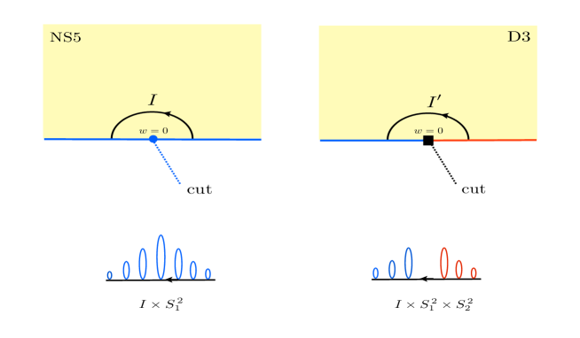
Figure 6: Local singularities corresponding to a NS5-brane (left) and a D3-brane (right), as explained in the text. The boundary of $\Sigma$ is colored red or blue according to which of the two 2-spheres, $S_{1}^{\,2}$ or $S_{2}^{\,2}$, shrinks at this part of the boundary to zero. The non-contractible cycles supporting the brane charges are $I\times S_{1}^{\,2}$, $I\times S_{1}^{\,2}\times S_{2}^{\,2}$ and $I^{\prime}\times S_{1}^{\,2}\times S_{2}^{\,2}$, with $I$ and $I^{\prime}$ the (oriented) solid semicircles of the figure. These cycles are topologically equivalent to a 3-sphere, a 3-sphere times a 2-sphere, and a 5-sphere. The broken lines indicate the logarithmic (on the left) and square root (on the right) branch cuts.

In addition to 5-brane charge, the singularities (3.19) also carry D3-brane charge. The corresponding flux threads the 5-cycle $I\times S_{1}^{\,2}\times S_{2}^{\,2}$, which is topologically the product of a 3-sphere with a 2-sphere. There is a well-known subtlety in the definition of this charge, because of the Chern-Simons term in the IIB supergravity action [5, 28, 29]. In the case at hand the conserved flux is the integral of the gauge-variant 5-form $F_{(5)}+C_{(2)}\wedge H_{(3)}$, which obeys a non-anomalous Bianchi identity. The number of D3-branes inside the NS5-brane stack is thus given by

$$\hat{N}_{3}\,=\,{1\over(4\pi^{2}\alpha^{\prime})^{2}}\int_{I\times S_{1}^{\,2}\times S_{2}^{\,2}}[F_{(5)}+C_{(2)}\wedge H_{(3)}]\,=\,-{2\over\pi\alpha^{\prime}}\,\hat{N}_{5}\,h_{1}^{D}\Bigl{|}_{w=0}\ .$$ (3.21)

It can be checked, by taking again $I$ arbitrarily small, that $F_{(5)}$, as well as all terms in the expression for $C_{(2)}$ other than $h_{1}^{D}$, do not contribute to the above flux. This explains the second equality, leading finally to

$$\hat{N}_{3}\,=\ \left({4\over\alpha^{\prime}}\right)^{2}\,\left({\hat{\gamma}\,\hat{c}\over\pi}\right)\ .$$ (3.22)

Note that $\hat{N}_{3}$ depends on the potential $C_{(2)}$ at the position of the 5-brane singularity, and may change under large gauge transformations. This is related to the Hanany-Witten effect [4], an issue to which we will return in the next subsection.

In principle, using $SL(2,\mathbb{R})$ transformations one can convert the NS5-brane solution to a more general $(p,q)$ fivebrane solution. Such transformations generate, however, a non-trivial Ramond-Ramond axion background, so $(p,q)$ fivebranes cannot coexist with the NS5-brane solution for which the axion vanishes. There is one exception to the rule: the S-duality transformation converts the NS5-brane to a D5-brane without generating an axion background. Combined with an exchange of the two 2-spheres, S-duality acts as follows on the harmonic functions:

$$\left(\begin{array}[]{c}i{\cal A}_{2}\\ -{\cal A}_{1}\end{array}\right)\ \xrightarrow{\tilde{S}}\ \left(\begin{array}[]{c}{\cal A}_{1}\\ i{\cal A}_{2}\end{array}\right)\ .$$ (3.27)

This gives the D5-brane singularity anticipated already in equation (3.19). The integer D5-brane and D3-brane charges read

$$N_{5}={4\over\alpha^{\prime}}\,\gamma\,,\qquad N_{3}\,=\ \left({4\over\alpha^{\prime}}\right)^{2}\,\left({\gamma\,c\over\pi}\right)\ .$$ (3.28)

Note that the D3-brane charge is here the flux of the 5-form $F_{(5)}-B_{(2)}\wedge F_{(3)}$, which is the S-duality transform of $F_{(5)}+C_{(2)}\wedge H_{(3)}$. This gauge-variant form is well-defined in any patch around the D5-brane singularity as long as this patch does not contain NS5-brane sources.

The last kind of singularity, which can coexist with D5- and NS5-brane singularities, is the one describing free D3-branes, with no associated fivebrane charge. In this case the holomorphic functions have square-root rather than logarithmic cuts [10]

$$\underline{\rm D3}:\qquad{\cal A}_{1}={1\over\sqrt{w}}(a_{1}+b_{1}w+\cdots)\ ,\qquad{\cal A}_{2}={1\over\sqrt{w}}(a_{2}+b_{2}w+\cdots)\ .$$ (3.29)

Such singularities change the boundary condition of $h_{1}$ from Neumann to Dirichlet, and the boundary condition of $h_{2}$ from Dirichlet to Neumann. This is illustrated in the right part of figure 6. The integer D3-brane charge is given by

$$n_{3}\,=\,{1\over\left(4\pi^{2}\alpha^{\prime}\right)^{2}}\int_{I^{\prime}\times S_{1}^{\,2}\times S_{2}^{\,2}}F_{(5)}\ =\ \left({4\over\alpha^{\prime}}\right)^{2}\,\,{(a_{1}b_{2}-a_{2}b_{1})\over 2\pi}\ .$$ (3.30)

The ten-dimensional geometry near the D3-brane singularity is an $AdS_{5}\times S^{5}$ throat with radius $L$ given by $L^{4}=4\pi\alpha^{\prime\,2}|n_{3}|$.

3.3 Linear-quiver geometries

Consider two harmonic functions with the singularity structure shown in figure 7. The corresponding geometries have the field-theory interpretation of superconformal domain walls in ${\cal N}=4,D=4$ super Yang Mills [23]. If $n_{3}^{\pm}$ are the D3-brane charges of the two boundary-changing (black-box) singularities, then the domain wall separates two gauge theories with gauge groups $U(n_{3}^{-})$ and $U(n_{3}^{+})$. As pointed out in [5, 6], one may decouple the three-dimensional SCFT that lives on the domain wall from the bulk four-dimensional Yang-Mills theories by setting $a_{j}^{\pm}=0$. Equation (3.29) shows that in this case $n_{3}^{+}=n_{3}^{-}=0$. The square-root singularities of the harmonic functions are then simply coordinate singularities, while the infinite $AdS_{5}\times S^{5}$ throats are replaced by regular interior points in ten-dimensions.

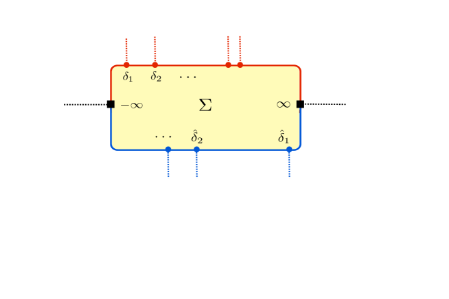
Figure 7: Structure of singularities of the harmonic functions for the linear-quiver geometries. The two boundary-changing singularities at $\pm\infty$, corresponding to $AdS_{5}\times S^{5}$ throats, can be capped off by choosing $a_{1}=a_{2}=0$, as described in the text. They become regular interior points of the ten-dimensional geometry.

Following references [30, 5, 6], we choose $\Sigma$ to be the infinite strip and the harmonic functions to be given by

$${\cal A}_{1}=-i\sum_{a=1}^{p}\gamma_{a}\ln\,\tanh\left(\frac{i\pi}{4}-\frac{z-\delta_{a}}{2}\right)\ ,\ \ \ {\cal A}_{2}=-\sum_{b=1}^{\hat{p}}\hat{\gamma}_{b}\ln\tanh\left(\frac{z-\hat{\delta}_{b}}{2}\right)\ .$$ (3.31)

Here $\delta_{1}<\delta_{2}<...<\delta_{p}$ are the positions of the D5-brane singularities on the upper boundary of the strip, whereas $\hat{\delta}_{1}>\hat{\delta}_{2}>...>\hat{\delta}_{\hat{p}}$ are the positions of the NS5-brane singularities on the lower boundary. It can be checked that on these two boundaries $h_{1}$ obeys, respectively, Neumann and Dirichlet conditions, while $h_{2}$ has Dirichlet and Neumann conditions. The boundary-changing square-root singularities are at $z=\pm\infty$. In the local coordinate $w=e^{\mp z}$ one can verify easily that $a_{j}^{\pm}=0$, so these points at infinity correspond to regular interior points of the ten-dimensional geometry.

To simplify the formulae we will adopt from now on the (non-standard) convention $\alpha^{\prime}=4$. Equations (3.28) and (3.20) give the numbers of NS5-branes and D5-branes for each fivebrane singularity:

$$N_{5}^{(a)}=\gamma^{(a)}\ ,\qquad\hat{N}_{5}^{(b)}=\hat{\gamma}^{(b)}\ .$$ (3.32)

Unbroken supersymmetry requires that there are only branes (or only anti-branes) of each kind. Thus all the $\gamma^{(a)}$ must have the same sign, and likewise for all the $\hat{\gamma}^{(b)}$. Dirac quantization forces furthermore these parameters to be integer.

Next let us consider the D3-brane charge. Inserting the harmonic functions (3.31) inside the expressions (3.28) and (3.22) gives

$$N_{3}^{(a)}=N_{5}^{(a)}\sum_{b=1}^{\hat{p}}\hat{N}_{5}^{(b)}\,{2\over\pi}{\rm arctan}(e^{\hat{\delta}_{b}-\delta_{a}})\ ,$$

$$\hat{N}_{3}^{(b)}=-\hat{N}_{5}^{(b)}\sum_{a=1}^{p}N_{5}^{(a)}\,{2\over\pi}{\rm arctan}(e^{\hat{\delta}_{b}-\delta_{a}})\ ,$$ (3.33)

where we used the identity $i\,$log tanh$({i\pi\over 4}-{x\over 2})=-$2 arctan($e^{x}$). As already noted in the previous subsection, this calculation of the D3-brane charge depends on the 2-form potentials $B_{(2)}$ and $C_{(2)}$ and is, a priori, ambiguous. One may indeed add a real constant to ${\cal A}_{1}$, or an imaginary constant to ${\cal A}_{2}$, thereby changing $h_{j}^{D}$ without affecting $h_{j}$. This gauge ambiguity is also reflected in the arbitrary choice of Riemann sheet for the logarithmic functions that enter in equations (3.31).

Following [5] we fix this ambiguity by placing all logarithmic cuts outside $\Sigma$, as in figure 7, and by choosing the sheet so that the imaginary part of (${\rm ln\,tanh}\,z$) vanishes when $z$ goes to $+\infty$ on the real axis. This implies that the arctangent functions take values in the interval $[0,\pi/2]$. Our choice of gauge is continuous in the interior of $\Sigma$ (which is covered by a single patch), and sets $B_{(2)}=0$ at $+\infty$ and $C_{(2)}=0$ at $-\infty$. With this choice, D5-branes at $\delta=+\infty$ and NS5-branes at $\hat{\delta}=-\infty$ do not contribute to the D3-brane charge. Placing, on the other hand, one NS5-brane at $\hat{\delta}=+\infty$ adds one unit of D3-brane charge to each D5-brane, while placing one D5-brane at $\delta=-\infty$ adds one unit of charge to each NS5-brane. This is a holographic manifestation of the Hanany-Witten effect.

Since this story will be important to us later, let us explain it a little more. The 2-form potential $B_{(2)}$ is proportional to the volume form ($\omega^{45}$) of the sphere $S_{1}^{\,2}$, which shrinks to a point in the lower boundary of the strip (the blue line in figure 7). When $B_{(2)}\not=0$, the corresponding boundary interval corresponds to a Dirac singularity of codimension 3 in (the 9-dimensional) space. This is unobservable if

$${1\over 2\pi\alpha^{\prime}}\int_{S_{1}^{\,2}}B_{(2)}\in 2\pi\mathbb{Z}\ \Longrightarrow\ B_{(2)}\Bigl{|}_{{\rm Im}z=0}\ =\ \pi\alpha^{\prime}\omega^{45}\times({\rm integer})\ .$$ (3.34)

With our choice of gauge,

$$B_{(2)}\Bigl{|}_{{\rm Im}z=0}\ =\ \pi\alpha^{\prime}\omega^{45}\times\sum_{b=1}^{\beta}\hat{N}_{5}^{(b)}\qquad{\rm for}\ \ \ \hat{\delta}_{\beta+1}<{\rm Re}z<\hat{\delta}_{\beta}\ .$$ (3.35)

Large gauge transformations change $B_{(2)}$ everywhere in the strip by a multiple of $\pi\alpha^{\prime}\omega^{45}$, and can remove the Dirac sheet in one of the intervals of the boundary. For us this was the interval $(\hat{\delta}_{1},\infty)$. A similar story holds also for the upper (red) boundary and the 2-form $C_{(2)}$. The D3-brane charges with our choice of gauge agree with the invariant linking numbers defined in §2.2.

The brane engineering of the dual gauge field theories [4, 23] involves $N$ D3-branes suspended between $\hat{k}$ NS5-branes on the left and $k$ D5-branes on the right. In the IIB supergravity the corresponding numbers are:

$$N=\sum_{a=1}^{p}N_{3}^{(a)}=-\sum_{b=1}^{\hat{p}}\hat{N}_{3}^{(b)}\ ,\qquad k=\sum_{a=1}^{p}N_{5}^{(a)}\ ,\qquad\hat{k}=\sum_{b=1}^{\hat{p}}\hat{N}_{5}^{(b)}\ .$$ (3.36)

The way in which the D3-branes are suspended to the five-branes is given by two partitions $\rho$ and $\hat{\rho}$, which define the linear-quiver gauge theory. These partitions are given in terms of the linking numbers:

$$\rho =\Big{(}\overbrace{l^{(1)},l^{(1)},..,l^{(1)}}^{N_{5}^{(1)}},\ \overbrace{l^{(2)},l^{(2)},..,l^{(2)}}^{N_{5}^{(2)}},\ ...\ ,\ \overbrace{l^{(p)},l^{(p)},..,l^{(p)}}^{N_{5}^{(p)}}\Big{)}\ ,$$

$$\hat{\rho} =\Big{(}\overbrace{\hat{l}^{(1)},\hat{l}^{(1)},..,\hat{l}^{(1)}}^{\hat{N}_{5}^{(1)}},\ \overbrace{\hat{l}^{(2)},\hat{l}^{(2)},..,\hat{l}^{(2)}}^{\hat{N}_{5}^{(2)}},\ ...\ ,\ \overbrace{\hat{l}^{(\hat{p})},\hat{l}^{(\hat{p})},..,\hat{l}^{(\hat{p})}}^{\hat{N}_{5}^{(\hat{p})}}\Big{)}\ ,$$ (3.37)

where $l^{(a)}=N_{3}^{(a)}/N_{5}^{(a)}$ and   $\hat{l}^{(b)}=\hat{N}_{3}^{(b)}/\hat{N}_{5}^{(b)}$. Here $l^{(a)}$ is the number of D3-branes ending on each D5-brane in the $a$th stack, while $\hat{l}^{(b)}$ is the number of D3-branes emanating from each NS5-brane in the $b$th stack. Because these numbers must be integers, the parameters $\delta_{a}$ and $\hat{\delta}_{b}$ are quantized. In all one has $2p+2\hat{p}-1$ parameters, since a global translation of all the $\delta_{a}$ and $\hat{\delta}_{b}$ does not change the solution. The parameters of the quiver are $N_{5}^{(a)},l^{(a)},\hat{N}_{5}^{(b)},\hat{l}^{(b)}$ subject to one constraint (3.36), which expresses the conservation of D3-brane charge. The two parameter counts therefore match.

The linking numbers of the supergravity solutions obey the inequalities $\rho^{T}>\hat{\rho}$, which were the conditions for the existence of a non-trivial infrared fixed point of the quiver gauge theory [23], see §2.2. On the supergravity side, the inequalities follow immediately [5] from the fact that $0<{\rm arctan}(x)<\pi/2$ for positive $x$. This is a non-trivial check of the AdS/CFT correspondence.

3.4 From strip to annulus

The strategy for constructing holographic IIB duals for the circular quivers is the following: one starts from the linear-quiver solutions that we have just described, and arranges the five-branes in infinite regular arrays. The holomorphic functions ${\cal A}_{j}$ become logarithms of quasi-periodic elliptic functions. Modding out by discrete translations then converts the strip domain, $\Sigma$, to an annulus, and the dual linear-quiver theories to theories based on circular quivers.

More explicitly, given a set of fivebrane singularities at $\delta_{a}$ and $\hat{\delta}_{b}$, we may always pick a positive parameter $t$ such that, after a rigid translation, $0\leq\delta_{a}\leq 2t$ and $0\leq\hat{\delta}_{b}\leq 2t$. Replicating the fivebrane sources with periodicity $2t$ then leads to the following harmonic functions

$$h_{1} =-\sum_{a=1}^{p}\gamma_{a}\ln\bigg{[}\prod_{n=-\infty}^{\infty}\tanh\bigg{(}\frac{i\pi}{4}-\frac{z-(\delta_{a}+2nt)}{2}\bigg{)}\bigg{]}+c.c.\ ,$$ (3.38)

$$h_{2} =-\sum_{b=1}^{\hat{p}}\hat{\gamma}_{b}\ln\bigg{[}\prod_{n=-\infty}^{\infty}\tanh\bigg{(}\frac{z-(\hat{\delta}_{b}+2nt)}{2}\bigg{)}\bigg{]}+c.c.\ .$$ (3.39)

These functions are manifestly periodic under translations by $2t$, so we are free to identify $z\equiv z+2t$ thereby converting the strip $\Sigma$ to an annulus. Figure 8 depicts this annular domain in the $w$-plane, where $w={\rm exp}({i\pi z/t})$.

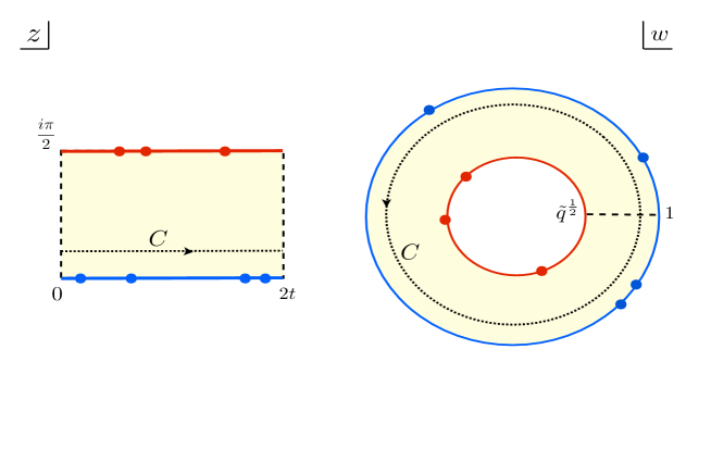
Figure 8: The annulus $\Sigma$ for the type-IIB solutions that are dual to $D=3,{\cal N}=4$ circular-quiver theories. $\Sigma$ is the infinite strip in the $z$ plane modulo the translations $z\to z+2t$ (left), or the annular domain in the $w={\rm exp}(i\pi z/t)$ plane (right). The radius of the inner boundary of the annulus is $\tilde{q}^{1/2}$ where $\tilde{q}={\rm exp}(-\pi^{2}/t)$ is the exponentiated dual modulus of the elliptic $\vartheta$-functions. The monodromies of $h_{j}^{D}$ around the curve $C$ give the total number of NS5 and D5-branes, as explained in the main text.

To see that the infinite products in the above expressions converge, we will rewrite them in terms of elliptic $\vartheta$-functions (we use the conventions of reference [31]). This can be done with the help of the identity

$$\Bigl{|}\frac{\vartheta_{1}(\nu|\tau)}{\vartheta_{2}(\nu|\tau)}\Bigr{|}\,=\,\left|\prod_{n=-\infty}^{\infty}\tanh(i\pi\nu+nt)\,\right|\ ,\qquad{\rm where}\quad e^{i\pi\tau}=e^{-t}\ .$$ (3.40)

The proof of this identity follows from the product formulae for the $\vartheta$-functions

$$\vartheta_{1}(\nu|\tau)=2e^{i\pi\tau/4}\sin(\pi\nu)\prod_{n=1}^{\infty}(1-e^{2ni\pi\tau})(1-e^{2ni\pi\tau}e^{2\pi i\nu})(1-e^{2ni\pi\tau}e^{-2\pi i\nu})\ ,$$ (3.41)

$$\vartheta_{2}(\nu|\tau)=2e^{i\pi\tau/4}\cos(\pi\nu)\prod_{n=1}^{\infty}(1-e^{2ni\pi\tau})(1+e^{2ni\pi\tau}e^{2\pi i\nu})(1+e^{2ni\pi\tau}e^{-2\pi i\nu})\ .$$ (3.42)

Note that the modular parameter is $\tau=it/\pi$, because the hyperbolic tangents are periodic under $z\to z+2\pi i$. Inserting the identity (3.40) in (3.38) leads to the following expressions for $h_{1}$ and $h_{2}$:

$$h_{1} =-\sum_{a=1}^{p}\gamma_{a}\ln\bigg{[}\frac{\vartheta_{1}\left(\nu_{a}|\tau\right)}{\vartheta_{2}\left(\nu_{a}|\tau\right)}\bigg{]}+c.c.\ ,\ \qquad{\rm with}\ \ \ i\,\nu_{a}=-\frac{z-\delta_{a}}{2\pi}+\frac{i}{4}\ ,$$ (3.43)

$$h_{2} =-\sum_{b=1}^{\hat{p}}\hat{\gamma}_{b}\ln\bigg{[}\frac{\vartheta_{1}\left(\hat{\nu}_{b}|\tau\right)}{\vartheta_{2}\left(\hat{\nu}_{b}|\tau\right)}\bigg{]}+c.c.\ ,\ \ \qquad{\rm with}\ \ \ i\,\hat{\nu}_{b}=\frac{z-\hat{\delta}_{b}}{2\pi}\ .$$ (3.44)

These harmonic functions are well-defined everywhere inside the annulus. They have logarithmic singularities on the boundaries, wherever $\nu_{a}$ or $\hat{\nu}_{b}$ vanish.

Decomposing $h_{j}$ into holomorphic and anti-holomorphic parts requires, as in the previous subsection, a choice of gauge. A convenient choice is to make the ${\cal A}_{j}$ analytic in the interior of the covering strip, before the periodic identification of $z$. This amounts to placing again all logarithmic branch cuts outside the strip. With this understanding, and recalling that the Jacobi $\vartheta$-functions are holomorphic, we have

$${\cal A}_{1}=-i\sum_{a=1}^{p}\gamma_{a}\ln\bigg{(}\frac{\vartheta_{1}\left(\nu_{a}|\tau\right)}{\vartheta_{2}\left(\nu_{a}|\tau\right)}\bigg{)}+\varphi_{1}\ ,\ \qquad{\cal A}_{2}=-\sum_{b=1}^{\hat{p}}\hat{\gamma}_{b}\ln\bigg{(}\frac{\vartheta_{1}\left(\hat{\nu}_{b}|\tau\right)}{\vartheta_{2}\left(\hat{\nu}_{b}|\tau\right)}\bigg{)}+i\varphi_{2}\ ,$$ (3.45)

where the constant phases $\varphi_{1}$ and $\varphi_{2}$ are residual quantized gauge degrees of freedom, corresponding to large gauge transformations of the 2-form potentials. As in the case of the linear quiver, we may use this residual freedom to enforce the absence of Dirac singularities in one interval on each annulus boundary.

Unlike $h_{j}$, the above holomorphic functions and the dual harmonic functions $h_{j}^{D}$ are not periodic under $z\to z+2t$. Their gauge-invariant holonomies (or Wilson lines) give the total fivebrane charges. To see why, note that translating $z\to z+2t$ changes all the arguments $\nu_{a}$ by $it/\pi$ (and all the $\hat{\nu}_{b}$ by $-it/\pi$). From the product formulae (3.41) one finds that under these translations the $\vartheta$-functions are quasi-periodic:

$$\vartheta_{1}(\nu+{it\over\pi}|\tau)=-e^{-2\pi i\nu+t}\vartheta_{1}(\nu|\tau)\ ,\qquad\vartheta_{2}(\nu+{it\over\pi}|\tau)=e^{-2\pi i\nu+t}\vartheta_{2}(\nu|\tau)\ .$$ (3.46)

The ratio $\vartheta_{1}/\vartheta_{2}$ changes only by a minus sign. Thus ln($\vartheta_{1}/\vartheta_{2})\to$ln($\vartheta_{1}/\vartheta_{2})\mp i\pi$ when $\nu\to\nu\pm it/\pi$, from which we conclude

$${\cal A}_{1}(z+2t)={\cal A}_{1}(z)-\pi\sum_{a=1}^{p}\gamma_{a}\ \,,\qquad{\cal A}_{2}(z+2t)={\cal A}_{2}(z)-i\pi\sum_{b=1}^{\hat{p}}\hat{\gamma}_{b}\ .$$ (3.47)

The meaning of these holonomies becomes clear if one integrates the 3-form field strengths over the 3-cycles $C\times S_{j}^{\,2}$, where $C$ is the dotted curve in figure 8. Consider for example the $H_{(3)}$ flux through $C\times S_{1}^{\,2}$. From equations (3.7) and (3.8) we deduce that this is proportional to

$$\oint_{C}db_{1}=2\oint_{C}dh_{2}^{D}\,=\,4i\,[{\cal A}_{2}(z+2t)-{\cal A}_{2}(z)]\ ,$$ (3.48)

where in the first step we used the fact that $(db_{1}-2dh_{2}^{D})$ is an exact differential which, therefore, integrates to zero. Since the total flux is conserved, the right-hand-side of (3.48) must be $z$-independent. Furthermore, by deforming the contour $C$ so that only the singularities on the outer boundary of the annulus contribute, one finds that the integrated flux is proportional to the total number of NS5-branes. This agrees with the holonomy of ${\cal A}_{2}$, as computed from the properties of the $\vartheta$-functions. The holonomy of ${\cal A}_{1}$ is likewise determined by the total number of D5-branes.

4 The AdS/CFT correspondence

We turn now to a discussion of the dictionary between the type-IIB supergravity solutions of the previous section, and the circular-quiver theories of section 2. As explained there, these gauge theories can be parametrized (in a redundant way) by the linking numbers of NS5-branes and D5-branes, and by the number $L$ of D3-branes that wind the circle. We will here first relate these numbers to the brane charges of the supergravity solutions, and then prove the basic inequalities (2.25). Modulo a few subtleties, this is a straightforward extension of the linear-quiver analysis of [5].

4.1 Calculation of D3-brane charges

The ten-dimensional geometries described in §3.4 have non-contractible three-cycles $I_{a}\times S^{\,2}_{2}$ and $\hat{I}_{b}\times S^{\,2}_{1}$, where $I_{a}$ is a semicircular curve around the $a$th singularity of $h_{1}$ on the upper annulus boundary, and $\hat{I}_{b}$ is a semicircle around the $b$th singularity of $h_{2}$ on the lower annulus boundary, see figure 9. These three-cycles are threaded respectively by R-R and NS-NS three-form fluxes, emanating from $\gamma_{a}$ D5-branes and from $\hat{\gamma}_{b}$ NS5-branes (in units where $\alpha^{\prime}=4$).

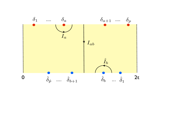
Figure 9: The non-contractible 5-cycles in the circular-quiver geometries are fibrations of the two 2-spheres over the curves shown in this figure. $\Sigma$ is an annulus, so the dotted boundaries are identified.

In addition, these geometries have a number of non-contractible five-cycles which can support D3-brane charge. These are fibrations of $S_{1}^{2}$ and $S_{2}^{2}$ over the three types of open curves $I_{a}$, $\hat{I}_{b}$ and $I_{ab}$ shown in figure 9. Recalling that $S_{1}^{2}$ shrinks to a point in the lower boundary, and $S_{2}^{2}$ shrinks to a point in the upper boundary of the annulus, one deduces that the topology of these 5-cycles is as follows:

• ${\cal C}_{a}^{5}\equiv(S_{1}^{2}\times S_{1}^{2})\ltimes I_{a}$ and $\hat{\cal C}_{b}^{5}\equiv(S_{1}^{2}\times S_{1}^{2})\ltimes\hat{I}_{b}$ are topologically $S^{3}\times S^{2}$;

• ${\cal C}_{ab}^{5}\equiv(S_{1}^{2}\times S_{1}^{2})\ltimes I_{ab}$ are topologically $S^{5}$ .

Here $I_{a}$ is a line segment semi-circling the $a$th singularity on the upper boundary, $\hat{I}_{b}$ likewise semicircles the $b$th singularity on the lower boundary, and $I_{ab}$ is a line segment which begins on the upper boundary of the annulus between the points $\delta_{a}$ and $\delta_{a+1}$ and ends on the lower boundary between the points $\hat{\delta}_{b}$ and $\hat{\delta}_{b+1}$. As shown in the figure, the orientation of the above segments is chosen to be counter-clockwise, or in the case of $I_{ab}$ from the upper annulus boundary to the lower boundary.

The D3-brane charges emanating from the five-brane singularities can be computed with the help of the general formulae of §3.2. Consider for example the $b$th NS5-brane stack which corresponds to the $z=\hat{\delta}_{b}$ singularity on the lower boundary of the annulus. Using $h_{1}^{D}={\cal A}_{1}+\bar{\cal A}_{1}$ and the expressions (3.21), (3.22) and (3.45) we find

$$\hat{N}^{(b)}_{3} =-\frac{2}{\pi\alpha^{\prime}}\hat{N}^{(b)}_{5}h_{1}^{D}|_{z={\hat{\delta}_{b}}}$$ (4.1)

$$=\hat{N}^{(b)}_{5}\,\sum_{a=1}^{p}N^{(a)}_{5}\,\left(\frac{i}{2\pi}\ln\bigg{[}\frac{\vartheta_{1}\left(\nu_{ab}|\tau\right)}{\vartheta_{1}\left(\bar{\nu}_{ab}|\tau\right)}\frac{\vartheta_{2}\left(\bar{\nu}_{ab}|\tau\right)}{\vartheta_{2}\left(\nu_{ab}|\tau\right)}\bigg{]}-\frac{4}{\pi\alpha^{\prime}}\varphi_{1}\right)\$$ (4.2)

where

$$i\nu_{ab}=\frac{\delta_{a}-\hat{\delta}_{b}}{2\pi}+\frac{i}{4}\ ,\qquad\tau=e^{-t}\ ,$$ (4.3)

and $\bar{\nu}$ is the complex conjugate of $\nu$. Likewise, one finds for the $a$th D5-brane:

$$N^{(a)}_{3} =\frac{2}{\pi\alpha^{\prime}}N^{(a)}_{5}h_{2}^{D}|_{z={\frac{i\pi}{2}+\delta_{a}}}$$ (4.4)

$$=N^{(a)}_{5}\,\sum_{b=1}^{\hat{p}}\hat{N}^{(b)}_{5}\,\left(-\frac{i}{2\pi}\ln\bigg{[}\frac{\vartheta_{1}\left(\nu_{ab}|\tau\right)}{\vartheta_{1}\left(\bar{\nu}_{ab}|\tau\right)}\frac{\vartheta_{2}\left(\bar{\nu}_{ab}|\tau\right)}{\vartheta_{2}\left(\nu_{ab}|\tau\right)}\bigg{]}-\frac{4}{\pi\alpha^{\prime}}\varphi_{2}\right)\ ,$$ (4.5)

where the arguments $\nu_{ab}$ are defined again by (4.3).

As has been discussed in the previous section, the D3-brane (Page) charge suffers from a gauge ambiguity which corresponds, in the above expressions, to the freedom in choosing the constants $\varphi_{1}$ and $\varphi_{2}$. In what follows, and until otherwise specified, we fix the gauge so that the potentials are continuous inside the fundamental domain $0\leq{\rm Re}z<2t$, and furthermore

$$C_{(2)} =0\qquad\rm{in}\ \ \,[0,\delta_{1}]\,\ \ \ \textrm{on the upper boundary},$$

$$B_{(2)} =0\qquad\rm{in}\,\ \ [\hat{\delta}_{1},2t]\,\ \ \ \textrm{on the lower boundary}.$$ (4.6)

The above choice can be motivated by considering the pinching limit $t\longrightarrow+\infty$ with $\delta_{a}-t$ and $\hat{\delta}_{b}-t$ kept fixed. In this limit the geometry degenerates to that of a linear quiver, and our gauge fixing agrees with the one adopted in reference [5].

Using the infinite-product expressions for the $\vartheta$-functions in (4.1) and (4.4), and fixing as just described $\varphi_{1}$ and $\varphi_{2}$, leads to the expressions

$${N^{(a)}_{3}}=N^{(a)}_{5}\sum_{b=1}^{\hat{p}}\hat{N}^{(b)}_{5}\Big{[}\sum_{n=0}^{+\infty}f(\hat{\delta}_{b}-\delta_{a}-2nt)-\sum_{n=1}^{+\infty}f(-\hat{\delta}_{b}+\delta_{a}-2nt)\Big{]}\ ,$$ (4.7)

and

$${\hat{N}^{(b)}_{3}}=\hat{N}^{(b)}_{5}\sum_{a=1}^{p}N^{(a)}_{5}\Big{[}\sum_{n=1}^{+\infty}f(-\hat{\delta}_{b}+\delta_{a}-2nt)-\sum_{n=0}^{+\infty}f(\hat{\delta}_{b}-\delta_{a}-2nt)\Big{]}\ ,$$ (4.8)

where ${N^{(a)}_{3}}$ is the D3-brane charge in the $a$th stack of D5-branes, ${\hat{N}^{(b)}_{3}}$ is the D3-brane charge in the $b$th stack of NS5-branes, and

$$f(x)=\frac{2}{\pi}\arctan(e^{x})\in[0,1]\ .$$ (4.9)

It can be easily verified that the above charges obey the sum rule

$$\sum_{a=1}^{p}N^{(a)}_{3}=-\sum_{b=1}^{\hat{p}}\hat{N}^{(b)}_{3}\ \equiv\ N\ .$$ (4.10)

In the pinching limit, where only the $n=0$ terms survive in the sums, all the $N^{(a)}_{3}$ are positive and all the $\hat{N}^{(b)}_{3}$ are negative numbers. For finite $t$, on the other hand, the numbers in each set can have either sign.

Next we consider the 5-cycles ${\cal C}_{ab}^{5}$. To associate to these 5-cycles a Page charge we must decide which (gauge-variant) 5-form to integrate. Take for instance the 5-form $\tilde{F}_{(5)}\equiv F_{(5)}+C_{(2)}\wedge H_{(3)}$, which obeys the non-anomalous Bianchi identity $d\tilde{F}_{(5)}=0$. This is globally defined only on the cycles ${\cal C}_{0b}^{5}$, since for all other choices of $a$, the gauge potential $C_{(2)}$ has a Dirac string singularity at the upper endpoint of $I_{ab}$. Put differently, $\int\tilde{F}_{(5)}$ would depend on the precise location of this upper endpoint unless $C_{(2)}=0$ in the corresponding boundary segment. By a similar reasoning one concludes that $\tilde{F}_{(5)}^{\prime}\equiv F_{(5)}-B_{(2)}\wedge F_{(3)}$ should be only integrated on the 5-cycles ${\cal C}_{a0}^{5}$. Both of these modified 5-forms can be integrated on the 5-cycle ${\cal C}_{00}^{5}$, which is picked out by our gauge fixing (4.1). Furthermore, the Page charge for this cycle does not depend on the choice of the modified 5-form since

$$\int_{{\cal C}_{00}^{5}}(\tilde{F}_{(5)}-\tilde{F}_{(5)}^{\prime})=\int_{{\cal C}_{00}^{5}}d\,(C_{(2)}\wedge B_{(2)})=0\ .$$ (4.11)

Let us denote the D3-brane charge for this special 5-cycle by $M$. If normalized appropriately, as in equation (3.21), $M$ must be an integer charge. We will now argue that this D3-brane charge is given by the following expression:

$$M=\sum_{a,b>0}N^{(a)}_{5}\hat{N}^{(b)}_{5}f(\hat{\delta}_{b}-\delta_{a})+\sum_{a,b\leq 0}N^{(a)}_{5}\hat{N}^{(b)}_{5}f(\delta_{a}-\hat{\delta}_{b})\ ,$$ (4.12)

where we here considered the universal cover of the annulus (i.e. the infinite strip), and extended the range of five-brane labels so that $-\infty<a<\infty$ is a label for the infinite array of D5-brane singularities from left to right, while $-\infty<b<\infty$ labels the corresponding array of NS5-brane singularities from right to left. Furthermore in this notation, $\delta_{a+np}\equiv\delta_{a}+2nt$ is the position of the $n$th image of the $a$th singularity on the upper strip boundary; likewise $\hat{\delta}_{b+m\hat{p}}\equiv\hat{\delta}_{b}-2mt$ corresponds to the $m$th image of the $b$th singularity on the lower strip boundary. The expression (4.12) can thus be written more explicitly as follows:

$$M =\sum_{a=1}^{p}\sum_{b=1}^{\hat{p}}N^{(a)}_{5}\hat{N}^{(b)}_{5}\Bigl{[}\sum_{m,n=0}^{\infty}f(\hat{\delta}_{b}-\delta_{a}-2nt-2mt)+\sum_{m,n=1}^{\infty}f(-\hat{\delta}_{b}+\delta_{a}-2nt-2mt)\Bigr{]}$$

$$=\sum_{a=1}^{p}\sum_{b=1}^{\hat{p}}N^{(a)}_{5}\hat{N}^{(b)}_{5}\sum_{s=1}^{\infty}s\Big{[}f(\hat{\delta}_{b}-\delta_{a}-2(s-1)t)+f(\delta_{a}-\hat{\delta}_{b}-2(s+1)t)\Big{]}\,.$$ (4.13)

A schematic explanation of the above expression is given in Figure 10.

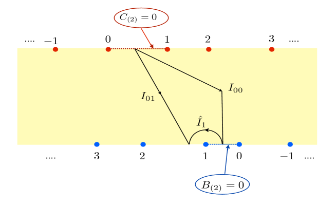
Figure 10: The infinite array of 5-brane singularities on the universal cover of the annulus. The D5-branes on the upper boundary are labelled from left to right, and the NS5-branes on the lower boundary from right to left. The choice of gauge determines a fundamental domain, and a special 5-cycle ${\cal C}_{00}^{5}=I_{00}\times S_{1}^{2}\times S_{2}^{2}$. The D3-brane charge supported by this cycle is obtained by summing over all pairs of singularities with positive labels, and all pairs with non-positive labels, see equation (4.12).

To see that (4.12) is indeed right, let us consider a change of gauge which makes $B_{(2)}$ vanish on the boundary segment between the $b=1$ and the $b=2$ singularities. The privileged 5-cycle is now ${\cal C}_{01}^{5}$, and the corresponding D3-brane charge $M^{\prime}$ reads

$$M^{\prime}=\sum_{a>0,b>1}N^{(a)}_{5}\hat{N}^{(b)}_{5}f(\hat{\delta}_{b}-\delta_{a})+\sum_{a\leq 0,b\leq 1}N^{(a)}_{5}\hat{N}^{(b)}_{5}f(\delta_{a}-\hat{\delta}_{b})\ .$$ (4.14)

The difference $M^{\prime}-M$ is equal to $\hat{N}^{(3)}_{1}$, the number of D3-branes in the first NS5-brane stack, as one can check with the help of equation (4.8). This should be so since $I_{01}=I_{00}\oplus\hat{I}_{1}$, as illustrated in Figure 10, and furthermore the corresponding Page charges, $M^{\prime}$ and $M+\hat{N}^{(3)}_{1}$, are given by integrals of the modified form $F_{(5)}+C_{(2)}\wedge H_{(3)}$ which does not depend on the choice of $B_{(2)}$ gauge.

This simple consistency check fixes almost uniquely the expression (4.12) for the charge $M$. To remove all doubts, we have also verified this formula numerically.

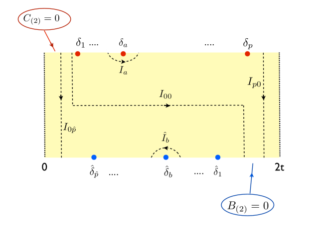
Figure 11: A fundamental domain and the segments $I_{0\hat{p}}$ and $I_{p0}$ which correspond to the Page charge $L$. This is the number of winding D3-branes, which vanishes in the (pinching) limit of a linear quiver.

Note that by deforming the open curves as in Figure 10 one can show that there are no independent charges besides $M$ and the Page charges $\{N^{(a)}_{5},\hat{N}^{(b)}_{5}\}$ of the five-branes. It will be convenient for our purposes here to trade $M$ for $L\equiv M-N$, where $N$ is the total charge carried by the D5-branes, see (4.10). The charge $L$ corresponds to the 5-form flux through the cycle ${\cal C}_{p0}^{5}$, or equivalently the cycle ${\cal C}_{0\hat{p}}^{5}$, depicted in Figure 11. Simple manipulations give

$$L\ =\ \sum_{a=1}^{p}\sum_{b=1}^{\hat{p}} N^{(a)}_{5}\hat{N}^{(b)}_{5}\sum_{n=0}^{\infty}\sum_{m=1}^{\infty}\Bigl{[}f(\hat{\delta}_{b}-\delta_{a}-2nt-2mt)+f(-\hat{\delta}_{b}+\delta_{a}-2nt-2mt)\Bigr{]}$$

$$=\sum_{a=1}^{p}\sum_{b=1}^{\hat{p}}N^{(a)}_{5}\hat{N}^{(b)}_{5}\sum_{s=1}^{\infty}s\Big{[}f(\hat{\delta}_{b}-\delta_{a}-2st)+f(\delta_{a}-\hat{\delta}_{b}-2st)\Big{]}\,.$$ (4.15)

Below, we will identify $L$ with the number of winding D3-branes in a circular quiver. Consistently with this interpretation, $L$ can be seen to vanish in the pinching limit, $t\to\infty$ with $\delta_{a}-\hat{\delta}_{b}$, for all $a=1,\cdots p$ and $b=1,\cdots\hat{p}$, held finite and fixed.

4.2 Parameter match

Following references [5, 6] we define the linking numbers of the fivebranes as the Page charge per five-brane in each given stack:

$$l^{(a)}\equiv\frac{N^{(a)}_{3}}{N^{(a)}_{5}}\ ,\quad\hat{l}^{(b)}\equiv-\frac{\hat{N}^{(b)}_{3}}{\hat{N}^{(b)}_{5}}\ ,\qquad{\rm with}\ \ \ \sum_{a=1}^{p}N^{(a)}_{5}l^{(a)}=\sum_{b=1}^{\hat{p}}\hat{N}^{(b)}_{5}\hat{l}^{(b)}=N\ .$$ (4.16)

We here assume that these linking numbers are integer. Strictly-speaking, Dirac’s quantization condition only requires integrality of the total charge for each five-brane stack, so solutions with fractional linking numbers cannot be ruled out a priori as inconsistent. We will nevertheless discard this possibility, because we have no candidate SCFTs on the holographically dual side with fractional linking numbers. But the question deserves further scrutiny.

Next let us identify the above liking numbers with those in the brane construction of the circular quivers described in §2.2, by defining the following two partitions of $N$:

$$\rho =\Big{(}\overbrace{l^{(1)},l^{(1)},..,l^{(1)}}^{N_{5}^{(1)}},\overbrace{l^{(2)},l^{(2)},..,l^{(2)}}^{N_{5}^{(2)}},...,\overbrace{l^{(p)},l^{(p)},..,l^{(p)}}^{N_{5}^{(p)}}\Big{)}\ ,$$

$$\hat{\rho} =\Big{(}\overbrace{\hat{l}^{(1)},\hat{l}^{(1)},..,\hat{l}^{(1)}}^{\hat{N}_{5}^{(1)}},\overbrace{\hat{l}^{(2)},\hat{l}^{(2)},..,\hat{l}^{(2)}}^{\hat{N}_{5}^{(2)}},...,\overbrace{\hat{l}^{(\hat{p})},\hat{l}^{(\hat{p})},..,\hat{l}^{(\hat{p})}}^{\hat{N}_{5}^{(\hat{p})}}\Big{)}\ .$$ (4.17)

Together with the additional parameter $L$, we thus have the exact same data that was used to define the circular-quiver gauge theories $C_{\rho}^{\hat{\rho}}(SU(N),L)$ . Put differently, the supergravity parameters $\{\gamma_{a},\delta_{a}\}$ can be used to vary the charges $\{N_{5}^{(a)},N_{3}^{(a)}\}$, the parameters $\{\hat{\gamma}_{b},\hat{\delta}_{b}\}$ can be used to vary $\{\hat{N}_{5}^{(b)},\hat{N}_{3}^{(b)}\}$, and the annulus modulus $t$ controls the number $L$ of winding D3-branes. One of the charges is not independent because of the sum rule (4.16), but this agrees precisely with the fact that the supergravity solution is invariant under a common translation of all five-brane singularities on the boundary of the annulus.

The parameter counts on the supergravity and gauge-theory sides therefore match. The quiver data, on the other hand, had to obey a set of inequalities in order for the theory to flow to a non-trivial IR fixed point, see section 2. We will show that the same inequalities are also obeyed on the supergravity side.

Note first that from the expressions (4.7) and (4.8), and the fact that $f(x)$ is a monotonic function, it follows that the linking numbers of the supergravity solutions are automatically arranged in decreasing order:

$$l^{(1)}>l^{(2)}>...>l^{(p)}\qquad{\rm and}\qquad\hat{l}^{(1)}>\hat{l}^{(2)}>...>\hat{l}^{(\hat{p})}\ .$$ (4.18)

From the brane-engineering point of view, it is possible to order the linking numbers by moving five-branes of the same type around each other in transverse space (this is obvious in the configuration of Figure 4). We have argued in section §2 that these moves do not change the infrared limit of the theory, up to decoupled free sectors. Such moves should thus be indistinguishable on the supergravity side.

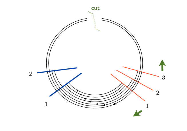
Figure 12: Brane engineering of a circular quiver. Cutting open the circle on its high side leads to the linking-number assignements $\rho=(3,1,1)$ and $\hat{\rho}=(3,2)$ with $L=2$; the corresponding theory is $C_{\rho}^{\hat{\rho}}(SU(5),2)$. The green arrows indicate the elementary D5-brane moves described in the text. For instance, a rotation of the $3$rd D5-brane changes these assignments to $\rho^{\prime}=(3,3,1)$ and $\hat{\rho}^{\prime}=(4,3)$ with $L^{\prime}=3$.

Besides being arranged in decreasing order, the linking numbers of the field-theory side could be furthermore chosen to lie in the intervals $(0,\hat{k}]$ and $(0,k]$, with $k$ and $\hat{k}$ respectively the total numbers of D5-branes and NS5-branes, see (2.19) and (2.24). As was explained in §2.2, these inequalities were automatic if one chose to cut open the circular chain at a link of locally-minimal rank. We will now explain why the same argument goes through on the supergravity side.

To this end, consider the circular quiver of Figure 12. Following the discussion in §2.2, to assign linking numbers to the five-branes we cut open the circular chain of D3-branes and then use the definitions (2.10). Clearly, the assignment is not unique since we are free to move one or several five-branes around the circle before cutting the chain. Let us focus, in particular, on the following two “elementary” moves:

• Move the (right-most) $k$th D5-brane anticlockwise, which produces the changes

  $$\Delta l_{k}=\hat{k}\ ,\ \ \Delta\hat{l}_{j}=1\ \ \ \forall\ j=1,\cdots\hat{k}\ ,\ \ \Delta L=l_{k}\ ;$$ (4.19)

• Move the (left-most) $1$rst D5-brane clockwise, which leads to the changes

  $$\Delta l_{1}=-\hat{k}\ ,\ \ \Delta\hat{l}_{j}=-1\ \ \ \forall\ j=1,\cdots\hat{k}\ ,\ \ \Delta L=\hat{k}-l_{1}\ .$$ (4.20)

These formulae translate the well-known fact that when a D5-brane crosses a NS5-brane it creates or destroys a D3-brane [4]. Similar formulae clearly hold for the mirror-symmetric moves of NS5-branes. The main point for us here is that the inequalities $l_{k}>0$ and $\hat{k}\geq l_{1}$ imply that $L$ is a “local” minimum with respect to elementary D5-brane moves. Likewise, $\hat{l}_{\hat{k}}>0$ and $k\geq\hat{l}_{1}$ imply that $L$ is a minimum with respect to elementary NS5-brane moves. One can thus impose the bounds (2.19) and (2.24) by choosing to cut the chain at a minimum of $L$.

This same line of argument applies to the supergravity side, where five-brane moves across the cut correspond to large gauge transformations. The elementary D5-brane moves are illustrated in Figure 13. They correspond to shifting the boundary segment on which $C_{(2)}=0$ to a neighboring segment, on the right or left. Pushing for example this segment to the left leads to the following transformations of charges:

$$\Delta l^{(p)}=\hat{k}\ ,\ \ \Delta\hat{l}^{(b)}=N_{5}^{(p)}\ \ \ \forall\ b\ ,\ \ \Delta L=N_{5}^{(p)}l^{(p)}\ .$$ (4.21)

The last two equations follow from the expression for the linking numbers (see §3.2) and from the argument illustrated in Figure 10. As for the first equation, it comes from the fact the $p$th D5-brane stack is replaced in the fundamental domain by the $0$th stack. On the universal cover of the annulus linking numbers (defined as the integrals over the 5-cycles ${\cal C}^{5}_{a}$ and $\hat{C}_{b}^{5}$) obey the periodicity conditions:

$$l_{a+np}=l_{a}-n\hat{k}\ ,\quad\hat{l}_{b+n\hat{p}}=\hat{l}_{b}-nk\ .$$ (4.22)

Thus replacing the $p$th stack by the $0$th stack changes the associated linking number by $\hat{k}$. Likewise, pushing the segment on which $C_{(2)}=0$ one step to the right leads to the following changes:

$$\Delta l^{(1)}=-\hat{k}\ ,\ \ \Delta\hat{l}^{(b)}=-N_{5}^{(1)}\ \ \ \forall\ b\ ,\ \ \Delta L=N_{5}^{(1)}(\hat{k}-l^{(1)})\ .$$ (4.23)

In this case the first D5-brane stack is replaced in the fundamental domain by the $(p+1)$th stack, as in Figure 13.

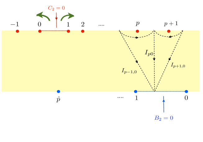
Figure 13: Global gauge transformations corresponding to the elementary D5-brane moves described in the text. Pushing the boundary segment on which $C_{(2)}=0$ one step to the right corresponds to moving the first stack of D5-branes around the circular quiver clockwise once. Pushing this boundary segment to the left corresponds to moving the last D5-brane stack once in the anti-clockwise direction.

Equations (4.21) and (4.23) are the same as (4.19) and (4.20) when $N_{5}^{(p)}=N_{5}^{(1)}=1$. The large gauge transformations are in this case the counterpart of the elementary D5-brane moves. More generally, they describe the effect of moving the first and last stacks of D5-branes around the circular quiver. Requiring that $L$ be minimum under these moves implies that $\hat{k}-l^{(1)}\geq 0$ and $l^{(p)}>0$, as advertized. Likewise one shows that $k-\hat{l}^{(1)}\geq 0$ and $\hat{l}^{(p)}>0$, by requiring minimality under changes of the $B_{(2)}$ gauge. That such a minimum exists is guaranteed by the fact that $L$ is bounded below, and goes to infinity along with the separation $\delta_{1}-\hat{\delta}_{1}$. Note that in general there are several minima, so different triplets of data $(\rho,\hat{\rho},L)$ may correspond to one and the same supergravity solution.

Having established the inequalities (2.19) and (2.24), we now need to prove the inequalities (2.25) for the associated Young tableaux. In the brane constructions of §2.2 these inequalities guaranteed that all gauge groups have positive rank, i.e. that they are realized on D3-branes rather than anti-D3-branes. This is a condition for supersymmetry, so we expect it to be automatically satisfied on the supergravity side. The proof is straightforward but tedious, and we relegate it to appendix B.

5 Limiting geometries

In this section we discuss the solutions described in §3.4, in regions of the parameters where the annulus with the marked points on the boundary degenerates. Note that taking $(\delta_{a}-\delta_{a+1})\to 0$ with $t$ held fixed merges the $a$th and $(a+1)$th stack of D5-branes. Modulo the subtle issue of linking number quantization, this limit is thus rather dull. The more interesting limits are those of an infinitely-thin or infinitely-fat annulus, $t\to\infty$ or $t\to 0$. We will comment on these two limits in turn.

5.1 Pinched annulus and wormbranes

When taking the limit $t\to\infty$ one must decide what to do with the positions, $\{\delta_{a}\}$ and $\{\hat{\delta}_{b}\}$, of the five-brane singularities. If the number of singularities is kept fixed then, since $\delta_{a}-\delta_{a+p}=\hat{\delta}_{b}-\hat{\delta}_{b+\hat{p}}=2t$, at least one of the intervals $\delta_{a}-\delta_{a+1}$ with $a\in[1,p]$, and at least one interval $\hat{\delta}_{b}-\hat{\delta}_{b+1}$ for some $b\in[0,\hat{p}-1]$ should become infinite in the limit. Without loss of generality, we take these divergent separations to correspond to $a=p$ and $b=0$. From the expression (4.1) we conclude that $L\to 0$ in this limit, so that the circular quiver degenerates to a linear quiver. If more than one interval diverges, the linear quiver breaks up further into disjoint linear quivers.

The linear-quiver geometries were analyzed in [5]. They are warped products $AdS_{4}\times_{w}K_{6}$, where $K_{6}$ is a compact manifold with singularities of co-dimension four at the locations of the five-branes. When $L$ is small (compared to all other D3-brane charges) but finite, the geometry describes what one may call a “worm-brane”. A schematic representation of this space-time is given in Figure 14. Two highly-curved $AdS_{5}\times S_{5}$ throats emanate from two distinct points of the compact space $K_{6}$, and are joined together to form a handle. The wormhole entrances are three-dimensional extended objects, whence the name “worm-brane”. Note that (in theories without exotic matter) point-like wormholes cannot be traversed and, in particular, they cannot provide short-cuts for time travel (see for instance [32, 33, 34]). Whether these conclusions can change in the case of worm-branes is an interesting question to which we may return in future work.

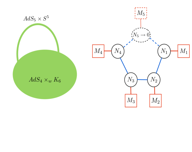
Figure 14: Breaking up of a circular quiver as described in the text. On the left, the ten-dimensional geometry describes a wormhole whose entrances are extremal D3-branes. An example of a dual gauge theory is illustrated on the right: a gauge-group factor with vanishing rank opens up the chain into a linear quiver.

From the perspective of the gauge theory, the pinching-limit geometries describe circular quivers with a gauge-group factor whose rank is much smaller than all other ranks. Taking this rank formally to zero opens up the circular chain, and decouples the corresponding fundamental hypermultiplets, see Figure 14. If several gauge-group ranks are made to vanish, the linear quiver breaks down into disjoint pieces. In general, the limiting geometries are smooth except when one sends a set of stacks of the same type infinitely far from all other stacks. This corresponds in gauge theory to the decoupling of free hypermultiplets from the end-points of a linear quiver. The geometry with five-branes of only one type is singular [5, 30], consistently with the fact that free hypermultiplets should have no smooth supergravity dual.

5.2 Large-$L$ limit and M2 branes

The second interesting limit of the circular-quiver solutions of section §3.4 is the limit $t\to 0$. As we will see, this is the limit of a very large number, $L$, of winding D3-branes, in which the five-branes are effectively smeared, and the solution reduces to the near-horizon geometry of M2-branes at a $Z_{k}\times Z_{\hat{k}}$ orbifold singularity.

To compute the geometry in this limit we use the asymptotic behavior of the theta functions when $e^{i\pi\tau}=e^{-t}\to 1$, or equivalently $e^{i\pi\tilde{\tau}}=e^{-i\pi/\tau}=e^{-\pi^{2}/t}\to 0$. One finds in this limit

$${\vartheta_{1}(\nu|\tau)\over\vartheta_{2}(\nu|\tau)}=-i{\vartheta_{1}(\nu\tilde{\tau}|\tilde{\tau})\over\vartheta_{4}(\nu\tilde{\tau}|\tilde{\tau})}\,=\ -2\,e^{-\pi^{2}/4t}\,{\rm sinh}({\pi^{2}\nu/t})+{\cal O}(e^{-9\pi^{2}/4t})\ ,$$ (5.1)

where the second equality follows from the expressions of the theta functions as infinite sums. The formula simplifies further if ${\rm Re}(\nu)\not=0$, in which case the hyperbolic sine can be replaced by an exponential. Inserting (5.1) in (3.45), and recalling that $2\pi{\rm Re}(\nu_{a})=\pi/2-{\rm Im}(z)$ and $2\pi{\rm Re}(\hat{\nu}_{b})={\rm Im}(z)$, finally gives

$${\cal A}_{1}\simeq\sum_{a=1}^{p}\gamma_{a}\,{\pi\over 2t}z+\varphi_{1}\ ,\ \quad{\cal A}_{2}=i\sum_{b=1}^{\hat{p}}\hat{\gamma}_{b}\,{\pi\over 2t}(z-{i\pi\over 2})+i\varphi_{2}\ ,$$ (5.2)

where we have absorbed some irrelevant constants in the arbitrary phases $\varphi_{1}$ and $\varphi_{2}$. This approximation breaks down at a distance $\sim t$ from the annulus boundaries, where the linear dependence is replaced by the rapidly-oscillating $\log\,{\rm sinh}$ function.

The first thing to note is that, away from the boundaries, the harmonic functions depend only on three parameters: $t$ and the total numbers of five-branes, $k=\sum\gamma_{a}$ and $\hat{k}=\sum\hat{\gamma}_{b}$. The precise locations of the five-brane singularities do not matter, as if these were smeared. It is convenient to scale out the $t$-dependence by redefining the annulus coordinate as follows: $2\pi z=2tx+i\pi^{2}y$, so that $x\in[0,2\pi)$ and $y\in[0,1]$. In terms of these coordinates, the holomorphic functions read

$${\cal A}_{1}\simeq k\,({x\over 2}+i{\pi^{2}y\over 4t})\ ,\ \quad{\cal A}_{2}=i\hat{k}\,\left({x\over 2}-\pi+i{\pi^{2}(y-1)\over 4t}\right)\ ,$$ (5.3)

where we have here chosen $\varphi_{1}$ and $\varphi_{2}$ so as to impose the canonical gauge condition (4.1). Inserting these functions in the general form of the solution, see §3.1, gives the Einstein-frame metric (we recall that $\alpha^{\prime}=4$):

$$ds^{2}=R^{2}g(y)^{1\over 4}\left[ds^{2}_{AdS_{4}}+y\,ds^{2}_{S^{2}_{1}}+(1-y)ds^{2}_{S^{2}_{2}}\right]+R^{2}g(y)^{-{3\over 4}}\left[{4t^{2}\over\pi^{4}}dx^{2}+dy^{2}\right]\ ,$$

$${\rm with}\quad R^{4}=\pi^{4}\,{{k\hat{k}}\over t^{2}}\ ,\qquad{\rm and}\quad g(y)=y(1-y)\ .$$ (5.4)

Furthermore, the dilaton and the non-vanishing gauge fields read:

$$e^{2\phi}=\frac{\hat{k}}{k}\sqrt{\frac{1-y}{y}}\ ,\qquad C_{(4)}=R^{4}\left({6tx\over\pi^{2}}\,\omega^{0123}+y^{2}(y-{3\over 2})\,\omega^{4567}\right)\ ,$$

$$B_{(2)}=2\hat{k}(2\pi-x)\,\omega^{45}\ ,\qquad C_{(2)}=-2kx\,\omega^{67}\ .$$ (5.5)

As already noted, this solution only depends on three integer parameters: the numbers $k$ and $\hat{k}$ of five-branes, and the modulus $t$ of the annulus which can be traded for the number of winding D3-branes via the formula (4.1),

$$L\,=\,\frac{k\hat{k}}{2t^{2}}\,\int_{0}^{+\infty}du\,u\,\frac{2}{\pi}\arctan(e^{-u})\,=\,\frac{\pi^{2}}{32}\,\frac{k\hat{k}}{t^{2}}\ .$$ (5.6)

One may also compare (4.1) to the formula (4.1) for the charge $M=L+N$, where $N$ gives the number of D3-branes emanating from five-branes. Since the summands in these two expressions differ by terms of order $t^{2}$, we conclude that $N\sim k\hat{k}$ as $t\to 0$. Thus the number of winding D3-branes far exceeds, in this limit, the number of D3-branes that end on the five-branes.

Not surprisingly, after having effectively smeared the five-branes, the solution has a Killing isometry under translations of the coordinate $x$. To be sure, $x$ enters in the expressions for $B_{(2)}$ and $C_{(2)}$ but this is a gauge artifact since the 3-form field strengths are $x$-independent. One may thus T-dualize the circle parametrized by $x$, using Buscher’s rules [35], to find a solution of type-IIA supergravity. This can be then lifted to eleven dimensions – the details of these calculations are given in appendix C. The final result for the eleven-dimensional metric is

$$ds_{{\rm M-theory}}^{2} ={\bar{R}^{2}}ds^{2}_{AdS_{4}}+\bar{R}^{2}\Big{[}4d\alpha^{2}+\sin^{2}\alpha\,ds^{2}_{S^{3}/\mathbb{Z}_{\hat{k}}}+\cos^{2}\alpha\,ds^{2}_{S^{3}/\mathbb{Z}_{k}}\Big{]}\ ,$$

$$ds^{2}_{S^{3}/\mathbb{Z}_{\hat{k}}} =d\theta_{1}^{2}+d\phi_{1}^{2}+4dx^{2}-4\cos\theta_{1}dxd\phi_{1}\ ,$$

$$ds^{2}_{S^{3}/\mathbb{Z}_{k}} =d\theta_{2}^{2}+d\phi_{2}^{2}+4dv^{2}-4\cos\theta_{2}dvd\phi_{2}\ ,$$ (5.7)

where $x$ and $v$ are angle coordinates with periodicities $x=x+2\pi/\hat{k}$ and $v=v+2\pi/k$, while the radius of $AdS_{4}$ is $\bar{R}^{2}=(2^{5}\pi^{2}k\hat{k}L)^{1/3}$.

This is the metric of $AdS^{4}\times S^{7}/(\mathbb{Z}_{k}\times\mathbb{Z}_{\hat{k}})$ with the two orbifolds acting on the two 3-spheres in $S^{7}$. The solution furthermore carries $L$ units of four-form flux. It can be recognized as the near-horizon geometry of $L$ M2-branes sitting at the fixed point of the orbifold $(\mathbb{C}^{2}/\mathbb{Z}_{\hat{k}})\times(\mathbb{C}^{2}/\mathbb{Z}_{k})$, where the orbifold identifications are

$$(z_{1},\bar{z}_{2})=e^{2i\pi/\hat{k}}(z_{1},\bar{z}_{2})\quad{\rm and}\quad(z_{3},\bar{z}_{4})=e^{2i\pi/k}(z_{3},\bar{z}_{4})\ .$$

Note that the two-forms $B_{(2)}$ and $C_{(2)}$ become, after the T-duality and the lift, part of the metric. This is in line with the fact that D5-branes transform to Kaluza-Klein monopoles, while T-duality in a transverse dimension maps the NS5-branes to ALE spaces with singularities of $A_{n}$ type [36, 18].

The superconformal field theories that are dual to M theory on $AdS^{4}\times S^{7}/(\mathbb{Z}_{k}\times\mathbb{Z}_{\hat{k}})$ are close relatives of the ABJM theory [37, 38] that have been analyzed by many authors, see for example [11, 12, 39, 13, 40, 16]. We will discuss them in more detail in the following section. Let us here only quote their free energy $F=-\log|Z|$ on the 3-sphere. Using the general formula of [40] one finds

$$F\,=\,L^{3/2}\sqrt{\frac{2\pi^{6}}{27\,{\rm Vol}_{7}}}\,=\,\frac{\pi}{3}\sqrt{2k\hat{k}}\,L^{3/2}\ ,$$ (5.8)

where ${\rm Vol}_{7}$ is the volume of the compact (Sasaki-Einstein) manifold whose metric is normalized so that $R_{ij}=6g_{ij}$. In the case at hand, this is the unit-radius seven sphere with orbifold identifications, so that ${\rm Vol}_{7}={\pi^{4}}/{3k\hat{k}}$.

As a check of our formulae, we may compute this free energy on the type-IIB side. Following [41], the on-shell IIB action can be computed via a consistent truncation to pure four-dimensional gravity with unit $AdS_{4}$ metric multiplied by a 6d volume factor. The explicit formula derived in [41] is

$$S_{\rm IIB}=-\frac{1}{(2\pi)^{7}(\alpha^{\prime})^{4}}\left(\frac{4}{3}\pi^{2}\right)(-6){\rm vol}_{6}\ ,$$ (5.9)

where for the solutions of interest

$${\rm vol}_{6}=-16(4\pi)^{2}t\int_{0}^{2\pi}\hskip-2.84526ptdx\int_{0}^{1}\hskip-2.84526ptdy\,h_{1}h_{2}\,\partial_{z}\partial_{\bar{z}}(h_{1}h_{2})\ .$$ (5.10)

Plugging in the harmonic functions $h_{1}=-i({\cal A}_{1}-\bar{\cal A}_{1})$ and $h_{2}={\cal A}_{2}+\bar{\cal A}_{2}$, and performing the integrals gives

$$S_{\rm IIB}=\frac{\pi^{4}}{48}\frac{k^{2}\hat{k}^{2}}{(2t)^{3}}=\frac{\pi}{3}\sqrt{2k\hat{k}}\,L^{3/2}$$ (5.11)

in perfect agreement with the result of M theory.

To summarize, we have shown here that when $L$ is large our solutions approach smeared backgrounds dual to M theory on $AdS^{4}\times S^{7}/(\mathbb{Z}_{k}\times\mathbb{Z}_{\hat{k}})$. In this limit the information about the positions of the five-branes is lost, and following [17, 19] its reinstatement would require non-trivial backgrounds for the wrapped-membrane field. The essential topological features of the background can be, however, in principle encoded more simply, as 3-form torsion of the M-theory orbifold [13, 14, 15, 16]. Note that, contrary to the $N>4$ cases studied in [38], the orbifolds considered here are not freely-acting on S$\hskip-1.42262pt\,{}^{7}$, and one would need to resolve their singularities. It would be interesting to work out the precise match of the torsion with the quiver data, and see how the constraints on the triplet $(\rho,\hat{\rho},L)$ arise from the M-theory side.

6 $SL(2,\mathbb{Q})$ and orbifold equivalences

Classical type-IIB supergravity has a continuous global $SL(2,\mathbb{R})$ symmetry [42] which transforms the axion-dilaton field, $S=\chi+ie^{-2\phi}$, and the NS-NS and R-R three-form field strengths as follows:

$$S^{\prime}={aS+b\over cS+d}\ ,\qquad\left(\begin{array}[]{c}\,\,H_{(3)}^{\prime}\\ F_{(3)}^{\prime}\end{array}\right)=\left(\begin{array}[]{cc}d&-c\\ -b&a\end{array}\right)\left(\begin{array}[]{c}\,H_{(3)}\\ F_{(3)}\end{array}\right)\ ,$$ (6.7)

where $a,b,c,d$ are real numbers with $ad-bc=1$. The transformations leave invariant the Einstein-frame metric, and the gauge-invariant five-form field strength.

As is well known, only the integer subgroup $SL(2,\mathbb{Z})$ is a symmetry of the full string theory [43], whereas continuous transformations can be used to generate inequivalent solutions. The authors of [9, 10] have indeed used such $SL(2,\mathbb{R})$ transformations to bring the general solution of the Killing-spinor equations to the local form given in §3.1. Conversely, acting with the transformations (6.7) generates new solutions from the ones of section 3, with singularities that correspond to general $(p,q)$ five-branes. We will now discuss briefly these new solutions.

6.1 Solutions with $(p,q)$ five-branes

The solutions given by the harmonic functions (3.31) or (3.43) have singularities on the upper boundary of the infinite strip or the annulus that correspond to D5-branes, and singularities on the lower boundary that correspond to NS5-branes. The charges are, respectively, $\gamma^{(e)}$ and $\hat{\gamma}^{(f)}$ for the stacks labeled by $e$ and $f$. Since the metric is invariant, the $SL(2,\mathbb{R})$ transformations do not change the positions and the total number of five-brane stacks. It transforms, however, their charges as follows

$$\gamma^{(e)}(0,1)\to\gamma^{(e)}(-c,a)\qquad{\rm and}\qquad\hat{\gamma}^{(f)}(1,0)\to\hat{\gamma}^{(f)}(d,-b)\ ,$$ (6.8)

where the NS5-brane and D5-brane charges are arranged as usual in a doublet. Let us write $(-c,a)=w(p,q)$ and $(d,-b)=\hat{w}(\hat{p},\hat{q})$, where $p,q$ and $\hat{p},\hat{q}$ are pairs of relatively-prime integers. Charge quantization requires that

$$N_{5}^{(e)\,\prime}=w\gamma^{(e)}\quad{\rm and}\quad\hat{N}_{5}^{(f)\,\prime}=\hat{w}\hat{\gamma}^{(f)}$$ (6.9)

be integer for all $e$ and $f$. Since the $\gamma$’s and $\hat{\gamma}$’s are arbitrary parameters, this can always be arranged to get any desired number of five-branes in each stack. The only conditions are that all five-branes on the upper boundary are of the same kind, including the sign, that the same is true for all five-branes on the lower boundary, and that furthermore these two kinds are different, $p\hat{q}-q\hat{p}\not=0$. This last constraint follows from the fact that the $SL(2,\mathbb{R})$ matrix has determinant one.

It should be stressed that the $SL(2,\mathbb{R})$ transformations take us, in general, outside the ansatz of §3.1; they generate in particular a non-vanishing R-R axion field. The only exception is S-duality ($S\to-1/S$) which interchanges the harmonic functions, and acts as mirror symmetry on the holographically-dual SCFT.

Consider next the D3-brane charges. These are not affected by $SL(2,\mathbb{R})$ transformations, provided one transforms the gauge choice covariantly. More explicitly, let us consider the D3-brane charge of the $(p,q)$ singularities in the upper boundary. The 2-form that has no component on $S_{2}^{2}$ [and is therefore well defined on a patch containing the whole upper boundary where this 2-sphere shrinks] is $B_{(2)}=aB_{(2)}^{\prime}+cC_{(2)}^{\prime}$. The D3-brane charge of a $(p,q)$ five-brane stack is given therefore by the integral of the following closed five-form

$$N_{3}^{(e)\,\prime}={1\over(4\pi\alpha^{\prime})^{2}}\int_{{\cal C}_{e}^{5}}\left[F_{(5)}-(aB_{(2)}^{\prime}+cC_{(2)}^{\prime})\wedge(bH_{(3)}^{\prime}+dF_{(3)}^{\prime})\right]\ ,$$ (6.10)

with the gauge choice $aB_{(2)}^{\prime}+cC_{(2)}^{\prime}=0$ in the lower-boundary segment $[\hat{\delta}_{1},2t]$. This is identical to the integral in the non-transformed solution, so that

$$N_{3}^{(e)\,\prime}=\gamma_{e}\sum_{f=1}^{\hat{p}}\hat{\gamma}_{f}\,\left(-\frac{i}{2\pi}\ln\bigg{[}\frac{\vartheta_{1}\left(\nu_{ef}|\tau\right)}{\vartheta_{1}\left(\bar{\nu}_{ef}|\tau\right)}\frac{\vartheta_{2}\left(\bar{\nu}_{ef}|\tau\right)}{\vartheta_{2}\left(\nu_{ef}|\tau\right)}\bigg{]}-\frac{4}{\pi\alpha^{\prime}}\varphi_{2}\right)\ ,$$ (6.11)

which is the same result as (4.4). The quantization of this charge puts the same constraints on the continuous parameters as in the untransformed solution. This is not however the case for the quantization of individual linking numbers, since the number $w\gamma^{(e)}$ of $(p,q)$ five-branes depends, via $w$, on the $SL(2,\mathbb{R})$ transformation.

Among all the solutions discussed here, those related by $SL(2,\mathbb{Z})$ transformations are physically equivalent [43]. To characterize inequivalent solutions, we may perform a $SL(2,\mathbb{Z})$ transformation that maps $(\hat{p},\hat{q})$ to $(1,0)$, so that the singularities on the lower boundary correspond to pure NS5-branes. Using then the shift symmetry $(p,q)\to(p+ql,q)$, which leaves invariant the NS5 branes, we can bring the second type of five-branes to a canonical form $(p,q)$ with $0\leq p<|q|$. The $SL(2,\mathbb{R})$ transformation from the ansatz of §3.1 to the above canonical form of the general solution is effected by the following matrix

$$\left(\begin{array}[]{cc}\hat{w}&-wp\\ 0&wq\end{array}\right)\quad{\rm with}\quad w\hat{w}q=1\ .$$ (6.14)

Multiplying (6.11) with $w\hat{w}q$, using (6.9) and the infinite-product expressions for the $\vartheta$-functions gives

$${N^{(a)\,\prime}_{3}}=qN^{(a)\,\prime}_{5}\sum_{b=1}^{\hat{p}}\hat{N}^{(b)\,\prime}_{5}\Big{[}\sum_{n=0}^{+\infty}f(\hat{\delta}_{b}-\delta_{a}-2nt)-\sum_{n=1}^{+\infty}f(-\hat{\delta}_{b}+\delta_{a}-2nt)\Big{]}\ ,$$ (6.15)

and likewise

$${\hat{N}^{(b)\,\prime}_{3}}=q\hat{N}^{(b)\,\prime}_{5}\sum_{a=1}^{p}N^{(a)\,\prime}_{5}\Big{[}\sum_{n=1}^{+\infty}f(-\hat{\delta}_{b}+\delta_{a}-2nt)-\sum_{n=0}^{+\infty}f(\hat{\delta}_{b}-\delta_{a}-2nt)\Big{]}\ .$$ (6.16)

A similar expression can be written for the winding charge $L^{\prime}$. Integrality of the linking numbers, $N^{(a)\,\prime}_{3}/N^{(a)\,\prime}_{5}$ and $\hat{N}^{(b)\,\prime}_{3}/\hat{N}^{(b)\,\prime}_{5}$, constraints the modulus $t$ and the positions of the singularities on the annulus boundary. When $q\not=1$ there are more allowed choices than in the case of pure D5-branes and NS5-branes.

The charges (6.15) and (6.16) obey the sum rule (4.10), and they thus still define two partitions $\rho$ and $\hat{\rho}$ of some integer $N$. Furthermore, these partitions still satisfy the basic inequalities (1.1). In general, we have no clear argument for why these conditions should be obeyed on the gauge-theory side. Indeed, for arbitrary $(p,q)$ there is no known Lagrangian description of the field theory (we refer the reader to section 8 of [44] for more details). Such a description only exists for the configurations involving $(1,k)$ 5-branes [44, 45, 11] : the $U(N)$ gauge theory living on a stack of $N$ D3-branes has level $k$ (or $-k$) Chern-Simons terms depending on whether the D3-branes end on the $(1,k)$ five-brane from the left (or the right).

6.2 Orbifold equivalences and free energies

An interesting corollary of the holographic dualities that we have presented in this work is the orbifold equivalence of different ${\cal N}=4$ superconformal gauge theories in three dimensions. Orbifold equivalences translate the fact that quantities which are sensitive only to the untwisted sector, are not affected by an orbifold operation [46, 47, 48]. Such quantities usually exist in the classical limit of string theory, and in the large-$N_{c}$ (planar) limit of gauge theories. An example of orbifold equivalence for the ABJM theory was analyzed recently in [51, 52]. Here we will present some more examples relating ${\cal N}=4$ circular-quiver theories.

The theories that we will discuss are related by $SL(2,\mathbb{R})$ transformations with rational entries, i.e. by elements of $SL(2,\mathbb{Q})$. Two theories related in this way are clearly equivalent in the limit where the supergravity approximation is valid, since $SL(2,\mathbb{R})$ is a symmetry of type-IIB supergravity. A similar rational extension of the perturbative T-duality group $O(d,d,\mathbb{Z})$ has been discussed recently in [21]. As explained in this reference, $O(d,d,\mathbb{Q})$ transformations can be seen as orbifold operations which lead to equivalences that are valid at any order in the $\alpha^{\prime}$ expansion. One may likewise view the $SL(2,\mathbb{Q})$ transformations as orbifold operations on the F-theory torus. This formal interpretation does not, however, imply in any obvious way that the equivalences presented here extend beyond the supergravity approximation.

The simplest example of “equivalent” theories are theories related by the $SL(2,\mathbb{Q})$ transformation

$$\left(\begin{array}[]{cc}r/s&0\\ 0&s/r\end{array}\right)\qquad{\rm with}\quad(r,s)\quad{\rm relatively\,prime\ integers}\,.$$ (6.19)

Such diagonal transformations do not modify the five-brane types, but they change the number of five-branes in each stack. They also transform their linking numbers, so as to leave unchanged the D3-brane charges:

$$\hat{N}^{(b)\,\prime}_{5}={r\over s}\,\hat{N}^{(b)}_{5}\,,\quad\hat{l}_{j}^{\,\prime}={s\over r}\,\hat{l}_{j}\,,\quad\quad N^{(a)\,\prime}_{5}={s\over r}\,N^{(a)}_{5}\,,\quad l_{i}^{\,\prime}={r\over s}\,l_{i}\,.$$ (6.20)

Consistency with charge quantization requires of course that $\hat{N}^{(b)}_{5}$ and $l_{i}$ be multiples of $s$, and that $N^{(a)}_{5}$ and $\hat{l}_{j}$ be multiples of $r$. Since the number, $L$, of winding D3-branes does not transform, whereas

$$k\to{s\over r}\,k\ \qquad{\rm and}\quad\hat{k}\to{r\over s}\,\hat{k}\ ,$$ (6.21)

the supergravity free energy (5.8) is invariant, as expected. Note that even these simple $SL(2,\mathbb{Q})$ transformations act highly non-trivially on the field theory side. For instance, the number of gauge-group factors is multiplied by $r/s$, while the total number of fundamental hypermultiplets is multiplied by $s/r$.

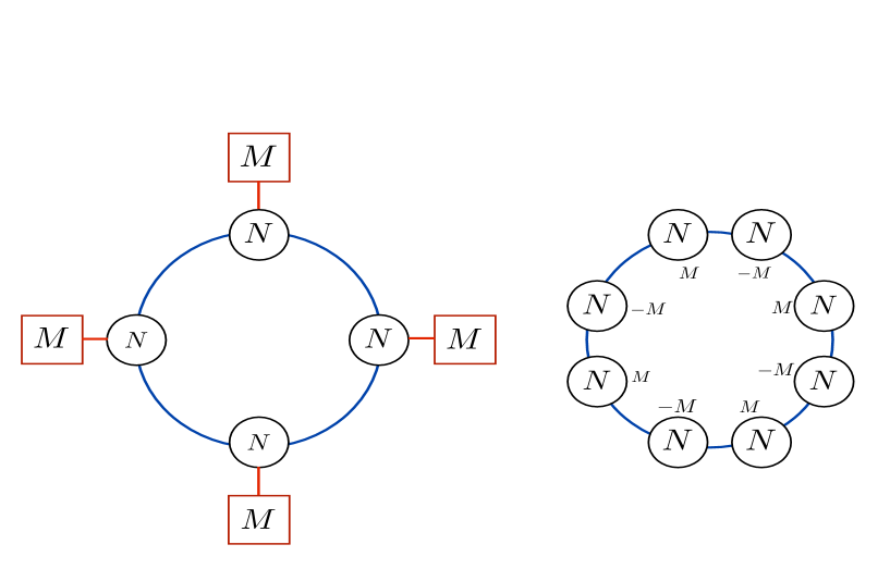
Figure 15: The two circular-quiver gauge theories related by the $SL(2,\mathbb{Q})$ transformation (6.24). The theory on the right is obtained from the one on the left by doubling the number of gauge-group factors, removing the fundamental hypermultiplets and adding Chern-Simons terms with alternating sign.

As another example of $SL(2,\mathbb{Q})$ equivalence, we consider the transformation

$$\left(\begin{array}[]{cc}1&M^{-1}\\ 0&1\end{array}\right)\qquad{\rm with}\quad M\in\mathbb{N}\,.$$ (6.24)

This transformation leaves the NS5-branes invariant, while it converts a stack of $M$ D5-branes to a single $(1,M)$ five-brane. Recall that the worldvolume theory of a stack of $N$ D3-branes intersecting a stack of $M$ D5-branes is a $U(N)$ gauge theory with $M$ fundamental hypermultiplets. Replacing the D5-branes by a $(1,M)$ five-brane leads to a $U(N)_{M}\times U(N)_{-M}$ gauge theory with a bifundamental hypermultiplet and level $M$ (respectively $-M$) Chern-Simons terms (see e.g. [37]). The transformation (6.24) can be used therefore to relate the following two theories:
(i) a $U(N)^{\hat{k}}$ gauge theory, with $M$ fundamental hypermultiplets for every gauge-group factor, and a bifundamental for each neighboring pair;
(ii) a $U(N)^{2\hat{k}}$ gauge theory with bifundamentals for each neighboring pair, and Chern-Simons terms of alternating level $\pm M$.
The corresponding circular quivers are illustrated in Figure 15. As a test of their $SL(2,\mathbb{Q})$ equivalence we will conclude this section by comparing the free energies of these two gauge field theories in the limit $N\gg 1$.

Let us first recall the result (5.8) for the free energy on the supergravity side. Replacing the number of winding D3-branes by $N$, and the total number of D5-branes by $M\hat{k}$, leads to the expression

$$F_{\rm sugra}\,=\,\frac{\pi\sqrt{2}}{3}\hat{k}M^{1/2}\,N^{3/2}\ .$$ (6.25)

This should be compared to the result on the field-theory side. For the necklace quiver of theory (ii) the calculation has been performed in [40]. These authors used the localization techniques of [53] to reduce the calculation to a matrix-model integral, which they then evaluated for large-$N$ by the saddle-point method. Their result agrees precisely with (6.25), confirming the AdS/CFT correspondence. What we need to do is to also recover this result from the original gauge theory (i).

Since for theories with ${\cal N}\geq 4$ supersymmetries the free energy does not run [53], we may perform the calculation near the (ultraviolet) Gaussian fixed point. Using the standard localization techniques, one reduces the partition function of theory (i) to the following matrix-model integral:

$$Z_{(i)}={1\over(N!)^{\hat{k}}}\int\prod_{a=1}^{\hat{k}}\frac{d^{N}\sigma_{a}}{(2\pi)^{N}}\frac{\prod_{i<j}4\sinh^{2}\big{(}\frac{\sigma_{a}^{i}-\sigma_{a}^{j}}{2}\big{)}}{\prod_{i,j}2\cosh\big{(}\frac{\sigma_{a+1}^{i}-\sigma_{a}^{j}}{2}\big{)}}\frac{1}{\big{[}\prod_{j}2\cosh\big{(}\frac{\sigma_{a}^{j}}{2}\big{)}\big{]}^{M}}\ ,$$ (6.26)

where $i,j$ run from $1$ to $N$. This can be written as $Z_{(i)}=\int e^{-F(\sigma_{a})}$ with

$$F(\sigma_{a})\,=\,-2\sum_{a\,;\,i<j}\log\Big{[}2\sinh\big{(}\frac{\sigma_{a}^{i}-\sigma_{a}^{j}}{2}\big{)}\Big{]}+\sum_{a\,;\,i,j}\log\Big{[}2\cosh\big{(}\frac{\sigma_{a+1}^{i}-\sigma_{a}^{j}}{2}\big{)}\Big{]}$$

$$+\sum_{a\,;\,j}M\log\Big{[}2\cosh\big{(}\frac{\sigma_{a}^{j}}{2}\big{)}\Big{]}+\hat{k}\log(N!)+\hat{k}N\log(2\pi)\ .$$ (6.27)

Following reference [40], we let $\sigma_{a}^{j}=N^{\beta}x_{a}^{j}$, and fix $\beta$ so that at the saddle point the $x_{a}^{j}$ are of order one. Contrary to this reference, we do not introduce an imaginary part for the $x_{a}^{j}$. Indeed, the saddle point equations are invariant under complex conjugation, so we are entitled to look for real solutions.

In the limit $N\gg 1$, we may replace the variables $x_{a}^{i}$ by a continuous density $\rho_{a}(x)$ normalized so that $\int dx\rho_{a}(x)=1$. The expression 6.27 can be written as

$$F(\rho_{a})=\sum_{a=1}^{\hat{k}} {1\over 2}\Big{[}{\pi^{2}}N^{2-\beta}\int dx_{a}\rho_{a}(x_{a})^{2}+{M}N^{1+\beta}\,\int dx_{a}|x_{a}|\rho_{a}(x_{a})\Big{]}$$ (6.28)

$$+O(N^{2-2\beta},N\log N)\ .$$

The details of the computation are subtle and can be found in appendix A of [40].

The saddle-point equations are non-trivial when the two terms in this expression are of the same order, so that $\beta=\frac{1}{2}$. Furthermore, thanks to the symmetries of the problem, we may look for saddle points with $\rho_{a}(x)=\rho(x)$ for all $a$, and $\rho(x)=\rho(-x)$. With these assumptions the above free energy reduces to

$$F(\rho)=\frac{\hat{k}}{2}N^{\frac{3}{2}}\Big{[}\pi^{2}\int dx\,\rho(x)^{2}+M\int dx\,|x|\rho(x)-\gamma\int dx\,\rho(x)+\gamma\Big{]}\ ,$$ (6.29)

where the Lagrange multiplier $\gamma$ imposes the constraint $\int dx\rho(x)=1$. The ensuing saddle point equation,

$$2\pi^{2}\rho(x)+M|x|=\gamma\ ,$$ (6.30)

is solved by the eigenvalue density

$$\rho(x) =\frac{1}{2\pi^{2}}\big{(}\gamma-M|x|\big{)}\quad\textrm{for}\quad|x|<x_{0},$$

$$=0\quad\textrm{for}\quad|x|>x_{0}.$$ (6.31)

The constraint $\int dx\rho(x)=1$ fixes the Lagrange multiplier

$$\gamma=\frac{Mx_{0}}{2}+\frac{\pi^{2}}{x_{0}}\ ,$$ (6.32)

whereas the positivity of $\rho$ implies $x_{0}\leq\pi\sqrt{\frac{2}{M}}$. Combining all these formulae gives

$$F(x_{0})=\hat{k}N^{\frac{3}{2}}\Big{[}\frac{\pi^{2}}{4x_{0}}+\frac{Mx_{0}}{4}-\frac{M^{2}x_{0}^{3}}{48\pi^{2}}\Big{]}\ .$$ (6.33)

We now need to minimize this expression with respect to $x_{0}$ which takes values in $(0,\pi\sqrt{{2/M}}]$. The minimum is achieved at the rightmost endpoint, leading to the final result for the gauge theory (i):

$$F_{(i)}=\frac{\pi\sqrt{2}}{3}\hat{k}\sqrt{M}N^{\frac{3}{2}}\ ,$$ (6.34)

in perfect agreement with both the necklace-quiver and the supergravity calculations. Note that although the final results agree, the three calculations differ greatly in their specific details.

Acknowledgements: We thank E. D’ Hoker, D. Jafferis, S. Pasquetti, J. Troost and M. Yamazaki for useful conversations. We are also indebted to the authors of [54] for drawing our attention to this reference. The research leading to these results has received funding from the [European Union] Seventh Framework Programme [FP7-People-2010-IRSES] under grant agreement n 269217. J.G. thanks the LPTENS for hospitality during this work. B.A. thanks the Perimeter Institute for hospitality during a visit. J.E. was supported by the FWO - Vlaanderen, Project No. G.0651.11, the “Federal Office for Scientific, Technical and Cultural Affairs through the Inter-University Attraction Poles Programme,” Belgian Science Policy P6/11-P, as well as the European Science Foundation Holograv Network, and is currently supported in part by STFC grant ST/J0003533/1. Research at the Perimeter Institute is supported in part by the Government of Canada through NSERC and by the Province of Ontario through MRI. J.G. also acknowledges further support from an NSERC Discovery Grant and from an ERA grant by the Province of Ontario.

Appendix A Mirror symmetry of inequalities

We will here show that the inequalities (2.25) are invariant under the mirror map, i.e. that

$$L+\rho^{T}>\hat{\rho}\ \ \Longleftrightarrow\ \ L+\hat{\rho}^{T}>\rho\ .$$ (A.1)

Let us first recall that if $\tau=(a_{1},a_{2},...,a_{t})$ and $\sigma=(b_{1},b_{2},...,b_{s})$ are two partitions of the same number $N$, expressed as vectors with non-increasing positive components, then $L+\tau>\sigma$ is a shorthand notation for the set of inequalities

$$L+\sum_{i=1}^{n}a_{i}>\sum_{i=1}^{n}b_{i}\quad\quad\textrm{for\ all }\quad n=1,...,\textrm{max}(t,s).$$ (A.2)

These can be visualized more easily in the diagrammatic representation of Figure 16, which defines a sequence $\{A_{1},A_{2},\cdots,A_{r}\}$ of areas with alternating signs. In terms of this sequence, the inequalities read

$$L+A_{1}>0\ ,\quad L+(A_{1}+A_{2})>0\ ,\quad\cdots\quad,\quad L>0\ ,$$ (A.3)

where the last inequality follows from the fact that $A_{1}+A_{2}\cdots+A_{r}=0$. Reversing the order, one may put these inequalities in the following form:

$$L-A_{s}>0\ ,\quad L-(A_{s}+A_{s-1})>0\ ,\cdots\quad,\quad L>0\ ,$$ (A.4)

or equivalently $L+\sigma^{T}>\tau^{T}$, as is evident if ones rotates by $90^{\rm o}$ Figure 16. Setting $\tau\equiv\rho^{T}$ and $\sigma\equiv\hat{\rho}$ proves the mirror equivalence (A.1), as claimed.

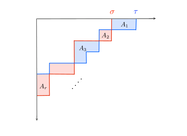
Figure 16: The difference of two Young tableaux defines an alternating sequence $\{A_{1},A_{2},\cdots,A_{r}\}$ where $|A_{i}|$ counts the number of boxes in the $i$th region enclosed by the two histograms of the Young tableaux. In this example $A_{1}=2,A_{2}=-1,A_{3}=3,\cdots$. The difference of the transposed tableaux, obtained by rotating the figure by $90^{\rm o}$, defines the inverse sequence $\{A_{r},\cdots,A_{2},A_{1}\}$.

Appendix B Proof of the inequalities in supergravity

We have already shown in §4.2 that, with an appropriate choice of gauge, the linking numbers of the supergravity solution can be confined to the intervals $\ l^{(a)}\in(0,\hat{k}]$ and $\hat{l}^{(b)}\in(0,k]$. In particular, the linking numbers are positive, and we demand that they be quantized. Thus the Young tableaux $\rho$ and $\hat{\rho}$ are well defined, and the inequalities $L+\rho^{T}>\hat{\rho}$ make sense. We will now prove that these inequalities are automatically obeyed on the supergravity side.

Let us recall the explicit expressions of the five-brane linking numbers and of $L$:

$$l^{(a)} =\sum_{b=1}^{\hat{p}}\hat{N}_{b}\Big{[}\sum_{n=0}^{+\infty}f(\hat{\delta}_{b}-\delta_{a}-2nt)-\sum_{n=1}^{+\infty}f(-\hat{\delta}_{b}+\delta_{a}-2nt)\Big{]}\ ,$$

$$\hat{l}^{(b)} =\sum_{a=1}^{p}N_{a}\Big{[}\sum_{n=0}^{+\infty}f(\hat{\delta}_{b}-\delta_{a}-2nt)-\sum_{n=1}^{+\infty}f(-\hat{\delta}_{b}+\delta_{a}-2nt)\Big{]}\ ,$$ (B.1)

$$L =\sum_{a=1}^{p}\sum_{b=1}^{\hat{p}}\sum_{k=1}^{+\infty}k\ N_{a}\hat{N}_{b}\Big{[}f(\hat{\delta}_{b}-\delta_{a}-2kt)+f(\delta_{a}-\hat{\delta}_{b}-2kt)\Big{]}\ ,$$

where $f(x)=\frac{2}{\pi}\arctan(e^{x})$, and we use in this appendix a lighter notation for the five-brane charges, $N_{a}\equiv N^{(a)}_{5}$ and $\hat{N}_{b}\equiv\hat{N}^{(b)}_{5}$. In terms of these linking numbers and the five-brane charges the partitions $\hat{\rho}$ and $\rho^{T}$ read:

$$\hat{\rho} =(\underbrace{\hat{l}^{(1)},...,\hat{l}^{(1)}}_{\hat{N}_{1}},...,\underbrace{\hat{l}^{(b)},...,\hat{l}^{(b)}}_{\hat{N}_{b}},...,\underbrace{\hat{l}^{(\hat{p})},...,\hat{l}^{(\hat{p})}}_{\hat{N}_{\hat{p}}})\ ,$$ (B.2)

and

$$\rho^{T}=(\underbrace{\sum_{a=1}^{p}N_{a},...,\sum_{a=1}^{p}N_{a}}_{l^{(p)}},\underbrace{\sum_{a=1}^{p-1}N_{a},...,\sum_{a=1}^{p-1}N_{a}}_{l^{(p-1)}-l^{(p)}},...,\underbrace{\sum_{a=1}^{A}N_{a},...,\sum_{a=1}^{A}N_{a}}_{l^{(A)}-l^{(A+1)}},...,\underbrace{N_{1},...,N_{1}}_{l^{(1)}-l^{(2)}})\ .$$ (B.3)

We need now to establish the set of inequalities

$$\sum_{s=1}^{r}m_{s}\ +L\ > \ \sum_{s=1}^{r}\hat{l}_{s}\qquad\forall r=1,\ldots,\max(k,\hat{k})\,.$$ (B.4)

where $\hat{\rho}=(\hat{l}_{1},\hat{l}_{2},...,\hat{l}_{\hat{k}})$ and $\rho^{T}=(m_{1},m_{2},...,m_{k})$ are the above two partitions.

The last inequality, the one for $r=\max(k,\hat{k})$, implies that $L>0$. This is obeyed automatically, as seen from the explicit expression (B) and the fact that $f$ is strictly positive. As in the case of the linear quivers, it is now sufficient to prove the inequalities (B.4) for the corners of the histogram $\hat{\rho}$, i.e. for the values

$$r=\sum_{b=1}^{J}\hat{N}_{b}\qquad{\rm where}\qquad J=1,2,...,\hat{p}\ .$$ (B.5)

We refer the reader to [5] for a detailed explanation of this claim. The above subset of inequalities takes the following explicit form:

$$\sum_{b=1}^{J}\hat{l}^{(b)}\hat{N}_{b}<L+\sum_{a=I+1}^{p}l^{(a)}N_{a}+\left(\sum_{a=1}^{I}N_{a}\right)\left(\sum_{b=1}^{J}\hat{N}_{b}\right)\ .$$ (B.6)

This is the form that we will prove using the supergravity calculation of the charges.

Let us give a name to the infinite sum that enters in the supergravity expressions for the linking numbers:

$$F(x,2t)\equiv\sum_{n=0}^{\infty}f(x-2nt)-\sum_{n=1}^{\infty}f(-x-2nt)\ .$$ (B.7)

In terms of the function $F$ the inequalities (B.6) can be written as

$$\sum_{a=1}^{p}\sum_{b=1}^{J}N_{a}\hat{N}_{b}\,F(\hat{\delta}_{b}-\delta_{a},2t)\ <\ L+\sum_{a=I+1}^{p}\sum_{b=1}^{\hat{p}}N_{a}\hat{N}_{b}\,F(\hat{\delta}_{b}-\delta_{a},2t)+\sum_{a=1}^{I}\sum_{b=1}^{J}N_{a}\hat{N}_{b}\ .$$

Splitting the sums, simplifying and rearranging terms gives:

$$\sum_{a=1}^{I}\sum_{b=1}^{J}N_{a}\hat{N}_{b}\,F(\hat{\delta}_{b}-\delta_{a},2t)-\sum_{a=I+1}^{p}\sum_{b=J+1}^{\hat{p}}N_{a}\hat{N}_{b}\,F(\hat{\delta}_{b}-\delta_{a},2t)\ <\ L+\sum_{a=1}^{I}\sum_{b=1}^{J}N_{a}\hat{N}_{b}\ .$$

We show that this is automatically satisfied by putting the following successive bounds on the left hand side:

$$\ \hskip 42.67912pt\sum_{a=1}^{I}\sum_{b=1}^{J}N_{a}\hat{N}_{b}\,F(\hat{\delta}_{b}-\delta_{a},2t)-\sum_{a=I+1}^{p}\sum_{b=J+1}^{\hat{p}}N_{a}\hat{N}_{b}\,F(\hat{\delta}_{b}-\delta_{a},2t)$$

$$\ \hskip 8.5359pt<\ \sum_{a=1}^{I}\sum_{b=1}^{J}N_{a}\hat{N}_{b}\,\sum_{n=0}^{\infty}f(\hat{\delta}_{b}-\delta_{a}-2nt)+\sum_{a=I+1}^{p}\sum_{b=J+1}^{\hat{p}}N_{a}\hat{N}_{b}\,\sum_{n=1}^{\infty}f(-\hat{\delta}_{b}+\delta_{a}-2nt)$$

$$< \ \sum_{a=1}^{I}\sum_{b=1}^{J}N_{a}\hat{N}_{b}\ f(\hat{\delta}_{b}-\delta_{a})\ +\ \sum_{a=1}^{p}\sum_{b=1}^{\hat{p}}N_{a}\hat{N}_{b}\ \sum_{n=1}^{\infty}\Big{[}f(\hat{\delta}_{b}-\delta_{a}-2nt)+f(-\hat{\delta}_{b}+\delta_{a}-2nt)\Big{]}$$

$$\ \hskip 108.12054pt<\ L+\sum_{a=1}^{I}\sum_{b=1}^{J}N_{a}\hat{N}_{b}\ .$$ (B.8)

In the first inequality we have dropped terms that are explicitly negative. The second inequality is obtained by extension of the sums. Finally, in the third inequatlity we used, in addition to the bound $0<f(x)<1$, the expression (B) for the winding charge $L$. This completes the proof.

Appendix C From IIB to M theory for large $L$

We give here the detailed T-duality transformation of the type-IIB solution for large winding number $L$ to a solution of type-IIA supergravity, and the subsequent uplift to eleven dimensions. We will follow the metric, dilaton and two-form gauge fields, which all become part of the metric in eleven dimensions. The four-form potential of the IIB theory transforms to the three-form potential of M theory, which at leading order has a field strength proportional to the ${\rm AdS}_{4}$ volume form. The way in which the 3-form field may encode the information on the five-brane throats is a very subtle issue, as already noted in the main text. We will not discuss it further in this appendix.

The type-IIB backgrounds in the large-$L$ limit are given by the expressions (5.4) and (5.5). In order to use the standard Buscher rules, we make a gauge transformation that removes the $x$-dependence from the gauge potentials. The new two-form potentials read

$$B_{(2)} =-2\hat{k}\,\cos(\theta_{1})dx\wedge d\phi_{1}\ ,\qquad C_{(2)}=-2k\,\cos(\theta_{2})dx\wedge d\phi_{2}\ ,$$

where we recall that $x$ is periodic with period $2\pi$. We also transform the Einstein-frame to the string-frame metric, $G_{MN}=e^{\phi}g_{MN}$, in terms of which Buscher’s rules read [35]:

$$G^{\prime}_{\mu\nu} =G_{\mu\nu}-\frac{G_{x\mu}G_{x\nu}-B_{x\mu}B_{x\nu}}{G_{xx}}\ ,\qquad G^{\prime}_{0\nu}=\frac{B_{x\mu}}{G_{xx}}\ ,\qquad G^{\prime}_{xx}=\frac{1}{G_{xx}}\ ,$$

$$B^{\prime}_{\mu\nu} =B_{\mu\nu}-\frac{G_{x\mu}B_{x\nu}-B_{x\mu}G_{x\nu}}{G_{xx}}\ ,\qquad B^{\prime}_{0\nu}=\frac{G_{x\mu}}{G_{xx}}\ ,\qquad e^{4\phi^{\prime}}=\frac{e^{4\phi}}{G_{xx}}\ ,$$ (C.1)

where the prime indicates the type-IIA fields in string frame, and the lower-case Greek indices $\mu,\nu$ run over all dimensions other than $x$. In addition, the 2-form R-R potential transforms to a one-form potential,

$$C^{\prime}_{(1)\mu} =C_{(2)x\mu}\ .$$ (C.2)

Since the IIB metric had no $(x\mu)$ components $B^{\prime}$ is zero, while the original 2-form NS-NS gauge field becomes an off-diagonal component of the IIA metric. In string-frame this latter reads:

$$dS_{{\rm IIA}}^{\,2}= {{\pi^{2}\hat{k}}\over t}\sqrt{1-y}\left[ds^{2}_{AdS_{4}}+y\,ds^{2}_{S^{2}_{1}}+(1-y)ds^{2}_{S^{2}_{2}}\right]$$

$$+{4\pi^{2}\over t}\sqrt{1-y}\left[{y\over\hat{k}}(dx-{\hat{k}\over 2}{\rm cos}\theta_{1}d\phi_{1})^{2}+\hat{k}{dy^{2}\over y(1-y)}\right]\ ,$$ (C.3)

whereas the R-R gauge field and the transformed dilaton field are given by

$$C_{(1)}^{\prime}=-2k\,\cos\theta_{2}d\phi_{2}\ ,\qquad e^{4\phi^{\prime}}={4\pi^{2}\over t}{\hat{k}\over k^{2}}(1-y)^{3/2}\ .$$ (C.4)

Finally we uplift the solution to M theory, whose metric (denoted here by a bar) is given in terms of the type-IIA backgrounds by the following relations [55]

$$\bar{g}_{MN}=e^{-4\phi^{\prime}/3}(G^{\prime}_{MN}+{1\over 4}e^{4\phi^{\prime}}C^{\prime}_{M}C^{\prime}_{N})\ ,\quad\bar{g}_{Mv}=e^{8\phi^{\prime}/3}C^{\prime}_{M}\ ,\quad\bar{g}_{vv}=4e^{8\phi^{\prime}/3}\ ,$$ (C.5)

where $v=v+2\pi$ parametrizes the eleventh dimension. Redefining the coordinates $x\rightarrow\hat{k}x$ , $v\rightarrow kv$ and $y=\sin^{2}\alpha$ gives, after some straightforward algebra, the $AdS^{4}\times S^{7}/(\mathbb{Z}_{k}\times\mathbb{Z}_{\hat{k}})$ metric, equation (5.2).

References

- [1] J. M. Maldacena, The Large N limit of superconformal field theories and supergravity, Adv.Theor.Math.Phys. 2 (1998) 231–252, [hep-th/9711200].
- [2] S. Gubser, I. R. Klebanov, and A. M. Polyakov, Gauge theory correlators from noncritical string theory, Phys.Lett. B428 (1998) 105–114, [hep-th/9802109].
- [3] E. Witten, Anti-de Sitter space and holography, Adv.Theor.Math.Phys. 2 (1998) 253–291, [hep-th/9802150].
- [4] A. Hanany and E. Witten, Type IIB superstrings, BPS monopoles, and three-dimensional gauge dynamics, Nucl.Phys. B492 (1997) 152–190, [hep-th/9611230].
- [5] B. Assel, C. Bachas, J. Estes, and J. Gomis, Holographic Duals of D=3 N=4 Superconformal Field Theories, JHEP 1108 (2011) 087, [arXiv:1106.4253].
- [6] O. Aharony, L. Berdichevsky, M. Berkooz, and I. Shamir, Near-horizon solutions for D3-branes ending on 5-branes, Phys.Rev. D84 (2011) 126003, [arXiv:1106.1870].
- [7] J. Gomis and C. Romelsberger, Bubbling Defect CFT’s, JHEP 0608 (2006) 050, [hep-th/0604155].
- [8] O. Lunin, On gravitational description of Wilson lines, JHEP 0606 (2006) 026, [hep-th/0604133].
- [9] E. D’Hoker, J. Estes, and M. Gutperle, Exact half-BPS Type IIB interface solutions. I. Local solution and supersymmetric Janus, JHEP 0706 (2007) 021, [arXiv:0705.0022].
- [10] E. D’Hoker, J. Estes, and M. Gutperle, Exact half-BPS Type IIB interface solutions. II. Flux solutions and multi-Janus, JHEP 0706 (2007) 022, [arXiv:0705.0024].
- [11] K. Hosomichi, K.-M. Lee, S. Lee, S. Lee, and J. Park, N=4 Superconformal Chern-Simons Theories with Hyper and Twisted Hyper Multiplets, JHEP 0807 (2008) 091, [arXiv:0805.3662].
- [12] M. Benna, I. Klebanov, T. Klose, and M. Smedback, Superconformal Chern-Simons Theories and AdS(4)/CFT(3) Correspondence, JHEP 0809 (2008) 072, [arXiv:0806.1519].
- [13] Y. Imamura and S. Yokoyama, N=4 Chern-Simons theories and wrapped M-branes in their gravity duals, Prog.Theor.Phys. 121 (2009) 915–940, [arXiv:0812.1331].
- [14] E. Witten, Branes, Instantons, And Taub-NUT Spaces, JHEP 0906 (2009) 067, [arXiv:0902.0948].
- [15] O. Aharony, A. Hashimoto, S. Hirano, and P. Ouyang, D-brane Charges in Gravitational Duals of 2+1 Dimensional Gauge Theories and Duality Cascades, JHEP 1001 (2010) 072, [arXiv:0906.2390].
- [16] A. Dey, On Three-Dimensional Mirror Symmetry, JHEP 1204 (2012) 051, [arXiv:1109.0407].
- [17] R. Gregory, J. A. Harvey, and G. W. Moore, Unwinding strings and t duality of Kaluza-Klein and h monopoles, Adv.Theor.Math.Phys. 1 (1997) 283–297, [hep-th/9708086].
- [18] D. Tong, NS5-branes, T duality and world sheet instantons, JHEP 0207 (2002) 013, [hep-th/0204186].
- [19] J. A. Harvey and S. Jensen, Worldsheet instanton corrections to the Kaluza-Klein monopole, JHEP 0510 (2005) 028, [hep-th/0507204].
- [20] K. Okuyama, Linear sigma models of H and KK monopoles, JHEP 0508 (2005) 089, [hep-th/0508097].
- [21] C. Bachas, I. Brunner, and D. Roggenkamp, A worldsheet extension of O(d,d:Z), arXiv:1205.4647.
- [22] M. R. Douglas and G. W. Moore, D-branes, quivers, and ALE instantons, hep-th/9603167.
- [23] D. Gaiotto and E. Witten, S-Duality of Boundary Conditions In N=4 Super Yang-Mills Theory, arXiv:0807.3720.
- [24] J. de Boer, K. Hori, H. Ooguri, Y. Oz, and Z. Yin, Mirror symmetry in three-dimensional theories, SL(2,Z) and D-brane moduli spaces, Nucl.Phys. B493 (1997) 148–176, [hep-th/9612131].
- [25] P. Kronheimer, Instantons and the geometry of the nilpotent variety, J.Diff.Geom. 32 (1990) 473–490.
- [26] C. Bachas, J. Hoppe, and B. Pioline, Nahm equations, N=1* domain walls, and D strings in AdS(5) x S(5), JHEP 0107 (2001) 041, [hep-th/0007067].
- [27] K. A. Intriligator and N. Seiberg, Mirror symmetry in three-dimensional gauge theories, Phys.Lett. B387 (1996) 513–519, [hep-th/9607207].
- [28] D. N. Page, Classical Stability of Round and Squashed Seven Spheres in Eleven-Dimensional Supergravity, Phys.Rev. D28 (1983) 2976.
- [29] D. Marolf, Chern-Simons terms and the three notions of charge, hep-th/0006117.
- [30] C. Bachas and J. Estes, Spin-2 spectrum of defect theories, JHEP 1106 (2011) 005, [arXiv:1103.2800].
- [31] M. B. Green, J. Schwarz, and E. Witten, Superstring theory. Vol. 2: Loop amplitudes, anomalies and phenomenology, .
- [32] M. Morris, K. Thorne, and U. Yurtsever, Wormholes, Time Machines, and the Weak Energy Condition, Phys.Rev.Lett. 61 (1988) 1446–1449.
- [33] M. Morris and K. Thorne, Wormholes in space-time and their use for interstellar travel: A tool for teaching general relativity, Am.J.Phys. 56 (1988) 395–412.
- [34] M. Visser, Lorentzian wormholes: From Einstein to Hawking, .
- [35] T. Buscher, Path Integral Derivation of Quantum Duality in Nonlinear Sigma Models, Phys.Lett. B201 (1988) 466.
- [36] H. Ooguri and C. Vafa, Two-dimensional black hole and singularities of CY manifolds, Nucl.Phys. B463 (1996) 55–72, [hep-th/9511164].
- [37] O. Aharony, O. Bergman, D. L. Jafferis, and J. Maldacena, N=6 superconformal Chern-Simons-matter theories, M2-branes and their gravity duals, JHEP 0810 (2008) 091, [arXiv:0806.1218].
- [38] O. Aharony, O. Bergman, and D. L. Jafferis, Fractional M2-branes, JHEP 0811 (2008) 043, [arXiv:0807.4924].
- [39] Y. Imamura and K. Kimura, On the moduli space of elliptic Maxwell-Chern-Simons theories, Prog.Theor.Phys. 120 (2008) 509–523, [arXiv:0806.3727].
- [40] C. P. Herzog, I. R. Klebanov, S. S. Pufu, and T. Tesileanu, Multi-Matrix Models and Tri-Sasaki Einstein Spaces, Phys.Rev. D83 (2011) 046001, [arXiv:1011.5487].
- [41] B. Assel, J. Estes, and M. Yamazaki, Large N Free Energy of 3d N=4 SCFTs and , arXiv:1206.2920.
- [42] J. H. Schwarz and P. C. West, Symmetries and Transformations of Chiral N=2 D=10 Supergravity, Phys.Lett. B126 (1983) 301.
- [43] C. Hull and P. Townsend, Unity of superstring dualities, Nucl.Phys. B438 (1995) 109–137, [hep-th/9410167].
- [44] D. Gaiotto and E. Witten, Supersymmetric Boundary Conditions in N=4 Super Yang-Mills Theory, arXiv:0804.2902.
- [45] D. Gaiotto and E. Witten, Janus Configurations, Chern-Simons Couplings, And The theta-Angle in N=4 Super Yang-Mills Theory, JHEP 1006 (2010) 097, [arXiv:0804.2907].
- [46] S. Kachru and E. Silverstein, 4-D conformal theories and strings on orbifolds, Phys.Rev.Lett. 80 (1998) 4855–4858, [hep-th/9802183].
- [47] A. E. Lawrence, N. Nekrasov, and C. Vafa, On conformal field theories in four-dimensions, Nucl.Phys. B533 (1998) 199–209, [hep-th/9803015].
- [48] M. Bershadsky, Z. Kakushadze, and C. Vafa, String expansion as large N expansion of gauge theories, Nucl.Phys. B523 (1998) 59–72, [hep-th/9803076].
- [49] A. Armoni, M. Shifman, and G. Veneziano, Refining the proof of planar equivalence, Phys.Rev. D71 (2005) 045015, [hep-th/0412203].
- [50] P. Kovtun, M. Unsal, and L. G. Yaffe, Necessary and sufficient conditions for non-perturbative equivalences of large N(c) orbifold gauge theories, JHEP 0507 (2005) 008, [hep-th/0411177].
- [51] M. Hanada, C. Hoyos, and A. Karch, Generating new dualities through the orbifold equivalence: a demonstration in ABJM and four-dimensional quivers, JHEP 1201 (2012) 068, [arXiv:1110.3803].
- [52] M. Hanada, C. Hoyos, and H. Shimada, On a new type of orbifold equivalence and M-theoretic duality, Phys.Lett. B707 (2012) 394–397, [arXiv:1109.6127].
- [53] A. Kapustin, B. Willett, and I. Yaakov, Exact Results for Wilson Loops in Superconformal Chern-Simons Theories with Matter, JHEP 1003 (2010) 089, [arXiv:0909.4559].
- [54] Y. Imamura, Monopole operators in N=4 Chern-Simons theories and wrapped M2-branes, Prog.Theor.Phys. 121 (2009) 1173–1187, [arXiv:0902.4173].
- [55] E. Witten, String theory dynamics in various dimensions, Nucl.Phys. B443 (1995) 85–126, [hep-th/9503124].