Sequence Annotation with HMMs:
New Problems and Their Complexity

Abstract

Hidden Markov models (HMMs) and their variants were successfully used for several sequence annotation tasks. Traditionally, inference with HMMs is done using the Viterbi and posterior decoding algorithms. However, recently a variety of different optimization criteria and associated computational problems were proposed. In this paper, we consider three HMM decoding criteria and prove their NP hardness. These criteria consider the set of states used to generate a certain sequence, but abstract from the exact locations of regions emitted by individual states. We also illustrate experimentally that these criteria are useful for HIV recombination detection.

Keywords:

Hidden Markov model, NP-hardness, sequence annotation, recombination detection

1 Introduction

Hidden Markov models (HMMs) and their variants were successfully used for several sequence annotation problems in bioinformatics, including gene finding, protein secondary structure prediction, protein family modeling, detection of conserved elements in multiple alignments and others (Burge and Karlin,, 1997; Krogh et al.,, 2001; Siepel et al.,, 2005; Sonnhammer et al.,, 1997). In many of these areas, we assume that a particular biological sequence $X$ was generated by the HMM, and we wish to infer which states of the model were used to generate particular parts of the sequence in a process called HMM decoding. The traditional algorithm for this task is the Viterbi algorithm (Viterbi,, 1967), which finds the state path (sequence of states) generating sequence $X$ with the highest probability.

Many other decoding criteria were proposed (Hamada and Asai,, 2012). For example, we can assign labels to states of the HMM, and then search for the most probable sequence of labels instead of the most probable state path. If multiple states can share the same label, this problem is NP-hard (Lyngsø and Pedersen,, 2002; Brejová et al.,, 2007) and heuristics are used in practice (Schwartz and Chow,, 1990; Krogh,, 1997). In effect, we use state labels to group together many state paths with the same meaning and then search for the group with the highest probability. In some application domains, it may be appropriate to group state paths together in different ways. In this paper, we explore three optimization problems of this kind.

Definition 1.1 (The most probable footprint)

The footprint of a state path (or labeling) is the list of states (or labels) visited on the path, discarding the information about the number of successive characters emitted by the same state (or label). The probability of a footprint is the sum of probabilities of all paths following the footprint. The task is to find the most probable footprint for a given HMM and sequence.

Definition 1.2 (The most probable set)

The set of a state path (or labeling) is the set of states (or labels) visited on the path, regardless of their order or multiplicity. The probability of a set is the sum of probabilities of all paths sharing the same set. The task is to find the set with the highest probability for a given HMM and sequence.

Definition 1.3 (The most probable restriction)

A path obeys a restriction (set of states or labels) if it uses only states or labels included in the restriction. The probability of a restriction is the sum of probabilities of all paths that obey the restriction. The task is to find the restriction of size $k$ with the highest probability for a given HMM and sequence.

These problems were motivated by the HIV recombination detection problem, which we review in Section 2. However, their use is not limited to this application and is appropriate wherever exact location of individual regions in the sequence is not important. We demonstrate usefulness of these problems in practice even if we use heuristics to solve them. Indeed, exact solution is unlikely, since in Sections 3, 4 and 5, we show that all three problems are NP-hard. The most probable footprint problem was briefly considered by Brown and Truszkowski, (2010), who observe that it is polynomially solvable in HMMs with two states or two labels. The other two problems were not studied previously.

Hidden Markov models and notation.

In the rest of this section, we introduce the necessary notation. A hidden Markov model (HMM) is a generative probabilistic model with a finite set of states $V$ and transitions $E$. The generative process starts by choosing a starting state $v_{1}$ according to the initial state probabilities $I(v_{1})$. Then in each round, the model emits a single symbol $x_{i}$ from the emission probability distribution $e(v_{i},x_{i})$ of the current state $v_{i}$, and then changes the state to $v_{i+1}$ according to the transition probability distribution $a(v_{i},v_{i+1})$. The process continues for some fixed number of steps $n$. Thus, the joint probability of generating a sequence $X=x_{1},\dots,x_{n}$ by a state path $\pi=v_{1},\dots,v_{n}$ in an HMM $H$ is $\Pr(\pi,X\mid H,n)=I(v_{1})\cdot e(v_{1},x_{1})\cdot\prod_{i=2}^{n}a(v_{i-1},v_{i})\cdot e(v_{i},x_{i})$. In other words, the HMM defines a probability distribution $\Pr(\pi,X\mid H,n)$ over all possible sequences $X$ and state paths $\pi$ of length $n$.

Let $Y$ be a sequence over some alphabet such that $Y=x_{1}^{k_{1}}x_{2}^{k_{2}}\dots x_{n}^{k_{n}}$ where $x_{i}$ and $x_{i+1}$ are distinct characters and each $k_{j}$ is greater than zero. Then the footprint $f(Y)$ of this sequence is $x_{1}x_{2}\dots x_{n}$ and its character set $s(Y)$ is $\{x_{1},x_{2},\dots x_{n}\}$ (note that the size of this set can be less than $n$). For example for $Y=aabaaacc$, we have $f(Y)=abac$ and $s(Y)=\{a,b,c\}$.

In particular, we will apply the footprint and set operators to state paths $\pi$. Probability of a footprint $F$ for a given HMM $H$ and sequence $X$ of length $n$ is

$$\Pr(f(\pi)=F,X\mid H,n)=\sum_{\pi,f(\pi)=F}\Pr(\pi,X\mid H,n).$$

Analogously we also define a probability of a given set of states $S$ denoted as $\Pr(s(\pi)=S,X\mid H,n)$. Note that each path $\pi$ included in this probability must use every state in $S$ at least once. Finally, we will also discuss the probability of a state restriction $S$ denoted as $\Pr(s(\pi)\subseteq S,X\mid H,n)$, where we count all state paths that use only states from set $S$, but are not required to use all of them.

We can also assign label $\ell(v)$ to each state $v$ of the HMM. The label $\ell(\pi)$ of a state path $\pi$ is then concatenation of labels for individual states on the path. We can then use similar notation for probability of footprints and sets defined on labelings, such as $\Pr(f(\ell(\pi))=F,X\mid H,n)$.

We will say that a state path $\pi$ can generate $X$ if $\Pr(\pi,X|H,n)>0$. Similarly a footprint $F$ can generate $X$ if $\Pr(f(\pi)=F,X\mid H,n)>0$ and a set of states $S$ can generate $X$ if $\Pr(s(\pi)=S,X\mid H,n)>0$.

2 Motivation

The problems studied in this paper were inspired by the HIV recombination detection problem, which was recently successfully approached with jumping HMMs (Schultz et al.,, 2006). In this setting, we represent sequence of each subtype of the HIV virus as a profile HMM, and then we combine these profiles to a single HMM by addition of special transitions modeling recombination between genomes of different strains of the virus. Given a particular genome, we try to establish which portions were generated by which profile. However, it is virtually impossible to determine the exact position of the recombination. Therefore we may wish to group together state paths that differ in positions of individual recombination points only by a small amount (Nánási et al.,, 2010; Brown and Truszkowski,, 2010; Truszkowski and Brown,, 2011).

In this scenario, each subtype corresponds to one label. Set of a labeling $s(\ell(\pi))$ corresponds to the set of subtypes present in the query sequence $X$. If we are not interested in the location of recombination points, this is the most natural measure to optimize. However, we might be interested to also know the order of subtypes along the sequence represented by the footprint of a labeling $f(\ell(\pi))$.

Additionally, we can use a multi-step decoding strategy, where we first fix a set of labels or a footprint, and then refine it to a full labeling by a secondary optimization criterion. This approach was taken by Truszkowski and Brown, (2011), mainly as a heuristic for speeding up the search. Here we show that this two-step strategy can be also useful for improving the prediction accuracy. In particular, as a second step we use the highest expected reward decoding (HERD) (Nánási et al.,, 2010). The method has two important parameters: window size $W$ (breakpoints within this distance are considered equivalent) and penalty $\gamma$ for false positives (each true positive breakpoint is scored $+1$, false positive breakpoint scores $-\gamma$). HERD optimizes expected value of this scoring function under the assumption that the sequence was generated from the HMM.

As we can see in Figure 2, the program is very sensitive to the choice of $\gamma$: for the optimal value of $\gamma$ it is significantly more accurate than the Viterbi algorithm, but if we increase $\gamma$ too much, the performance deteriorates. The most common problem is that HERD predicts too many breakpoints when $\gamma$ is low (Figure 1). By fixing a footprint as a constraint in the two-step strategy, and then optimizing the HERD criterion only for labelings obeying this footprint, the prediction accuracy is virtually independent of $\gamma$ and relatively close to the optimum values. Fixing the set instead of the footprint yields slightly higher specificity and lower sensitivity compared to optimizing HERD directly. Note that the footprints and sets are chosen by a simple heuristic; perhaps even better results could be obtained with optimal choice of these constraints.

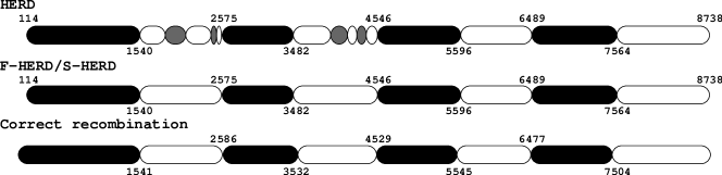
Figure 1: Prediction of recombination on artificial recombinant of subtypes $A$ and $B$ (black and white) with recombination every 950-1050 bases. HERD decoding yielded regions associated with incorrect subtypes (gray color representing 3 different subtypes) and fixing either the set or the footprint improved accuracy.

Figure 2: Feature specificity (a) and sensitivity (b) as a function of parameter $\gamma\in[0.1,2]$ on a semi-artificial set. A feature is correctly predicted if its boundaries are within 30 symbols of the corresponding feature in the correct annotation. Sensitivity is the proportion of real features that were correctly predicted and specificity is the proportion of predicted features that are correct. We use HERD parameters $P_{j}=10^{-5}$ and $W=10$. F-HERD optimizes the same criterion among labelings obeying the footprint obtained by sampling several paths from the probability distribution $\Pr(\pi\mid X,H,n)$, computing the footprint for each path, and then taking the most frequently occurring footprint among the samples, using the software by Truszkowski and Brown, (2011). S-HERD optimizes HERD criterion among labelings using only labels from this footprint. The data set consists of 150 artificial recombinants of members of various subtypes of HIV virus with recombination every 200-300 residues.

3 The Most Probable Footprint

As previously seen, finding the most probable footprint is a reasonable decoding criterion, and it may also serve as a starting point in a multi-stage strategy. In this section we show that this problem is NP-hard. In particular, we will consider the footprint of a state path $f(\pi)$. The problem of optimizing the footprint of a labeling $f(\ell(\pi))$ is also NP-hard, because optimizing $f(\pi)$ is its special case, equivalent to optimizing $f(\ell(\pi))$ in an HMM in which each state has a unique label.

Theorem 3.1

There is a fixed HMM $H$ such that the following problem is NP-complete: Given a sequence $X$ of length $n$ and probability $p\in[0,1]$, determine if there is a footprint $F$ such that $\Pr(f(\pi)=F,X\mid H,n)\geq p$.

• We will prove NP-hardness by a reduction from the maximum clique problem using the HMM in Figure 3 with eight states and alphabet $\Sigma=\{S,S^{\prime},T,T^{\prime},\#,0,1,?\}$.

  

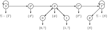
  Figure 3: The HMM from the proof of Theorem 3.1. Each circle denotes one state. The HMM always starts in state $S$. Under each state is the set of symbols that the state emits with non-zero probability. Each of these symbols is emitted with probability $1/k$, where $k$ is the size of the set. Alternatively, all outgoing transitions from a particular state have the same probability.

Let $G=(V,E)$ be an undirected graph with $n$ vertices $V=\{1,2,\dots,n\}$. We will encode it in a sequence $X$ over alphabet $\Sigma$ as follows. For every vertex $v\in V$, we create a block $X_{v}$ with $2n+3$ symbols: $X_{v}=S^{\prime}\#b_{v,1}\#b_{v,2}\#\dots\#b_{v,n}\#T^{\prime}$ where $b_{i,j}=1$ if $i=j$, $b_{i,j}=?$ if $(i,j)\in E$ and $b_{i,j}=0$ otherwise. Sequence $X$ is a concatenation of blocks for all vertices with additional first and last symbols: $X=SX_{1}X_{2}\dots X_{n}T$.

All state paths that can generate $X$ have a similar structure. The first symbol $S$ and several initial blocks are generated in state $S$, one block, say $X_{i}$, is generated in states $S^{\prime}$, $\#$, $0$, $1$, and $T^{\prime}$ and the rest of the sequence, including the final symbol $T$ is generated in state $T$. We will say that a state path with this structure covers the block $X_{i}$. Note that state $E$ is never used in generating $X$, its role is to ensure that the probability of self-transition is the same in states $S$ and $T$. All state paths that can generate $X$ have the same probability $q=\Pr(\pi,X\mid H,|X|)=2^{-2n^{2}-2n}3^{-n-1}7^{-2n^{2}-n+1}$.

We say that a state path $\pi$ is a run of footprint $F$, if $\pi$ can generate $X$, and $f(\pi)=F$. Every footprint $F$ that can generate $X$ has the following structure: $F=SS^{\prime}\#c_{1}\#c_{2}\#\dots\#c_{n}\#T^{\prime}T$ where $c_{i}\in\{0,1\}$. The probability of footprint $F$ is $qk$ where $k$ is the number of its runs. Also note that every run of $F$ covers a different $X_{i}$, because once $X_{i}$ is known, the whole path is uniquely determined.

We will now prove that the graph $G$ has a clique of size at least $k$ if and only if there is a footprint for sequence $X$ with probability at least $qk$. First, let $R$ be a clique in $G$ of size at least $k>0$. Consider the footprint $F=SS^{\prime}\#c_{1}\#c_{2}\#\dots\#c_{n}\#T^{\prime}T$ where $c_{i}=1$ if $i\in R$ and $c_{i}=0$ otherwise. For any $i\in R$, there is a run $\pi_{i}$ of $F$ that covers $X_{i}$. This run will use state 1 for generating each $b_{i,j}$ such that $j\in R$ and thus both $b_{i,j}\in\{?,1\}$ and $c_{j}=1$. For $j\notin R$ we have $b_{i,j}=0$ and $c_{j}=0$, thus they will use state 0 in $\pi$. Since there is a different run for every $i\in R$, footprint $F$ has at least $k$ runs.

Conversely, let $F$ be a footprint with probability at least $qk>0$ and thus with at least $k$ runs. We will construct a clique of size at least $k$ as follows. Let $R$ be the set of all vertices $i$ such that $f$ has a run that covers $X_{i}$. Clearly the size of $R$ is at least $k$. Since $F$ has non-zero probability, it has the form $SS^{\prime}\#c_{1}\#c_{2}\dots\#c_{n}\#T^{\prime}T$ for $c_{i}\in\{0,1\}$. For all $i\in R$, $c_{i}=1$ because the $i$-th block has $b_{i,i}=1$. Therefore for all $i,j\in R$, we have $b_{i,j}\in\{1,?\}$, which means that $(i,j)\in E$ or $i=j$. This implies that $R$ is indeed a clique.

To summarize, given graph $G$ and threshold $k$, we can compute in polynomial time sequence $X$ and threshold $qk$ such that $G$ has a clique of size at least $k$ if and only if sequence $X$ has a footprint with probability at least $qk$. This completes our reduction.

The problem is in NP (even if HMM is not fixed, but given on input), because given an HMM $H$, sequence $X$ and a footprint $F$, we can compute the probability $\Pr(f(\pi)=F,X\mid H,|X|)$ in polynomial time by a dynamic programming algorithm which considers all prefixes of $X$ and all prefixes of $F$. If probability $p$ and parameters of HMMs are given as rational numbers, we can compute all quantities without rounding in polynomial number of bits.       

4 The Most Probable Set of States

In this section, we prove NP-hardness of finding the most probable set of states. Again, as with footprint, this is a special case of the problem of finding the most probable set of labels.

Theorem 4.1

The following decision problem is NP-hard: Given an HMM $H$, sequence $X$ of length $n$, and a number $p\in[0,1]$, decide if there exists a set of states $S$ such that $\Pr\left(s(\pi)=S,X\mid H,n\right)\geq p$.

To prove this theorem, we will use a reduction from the maximum clique problem. Given a graph $G=(V,E)$ and a clique size $k$, we first choose a suitable threshold $k^{\prime}\geq k$, as detailed below, and construct a graph $G^{\prime}=(V^{\prime},E^{\prime})$ such that $G^{\prime}$ has a clique of size $k^{\prime}$ if and only if $G$ has a clique of size $k$. This is achieved simply by adding $k^{\prime}-k$ new vertices and connecting each of the new vertices to all other vertices in $V^{\prime}$. As long as $k^{\prime}-k$ is not too large, this transformation can be done in polynomial time.

In the next step, we use $G^{\prime}$ and $k^{\prime}$ to construct an HMM, an input sequence and a probability threshold. We will use the following straightforward way of converting a graph to an HMM.

Definition 4.1

Let $G=(V,E)$ be an undirected graph (without self-loops). Then the graph HMM $H_{G}$ is defined as follows:

• Its set of states is $V\cup\{\psi\}$, where $\psi\notin V$ is a new state called the error state.

• Its emission alphabet is $\{0,1\}$.

• Each state $v\in V$ has initial probability $I(v)=1/|V|$, the error state has initial probability $I(\psi)=0$.

• Each state $v\in V$ emits 0 with probability 1, the error state emits 1 with probability 1.

• Transitions with non-zero probability between states $u,v\in V$ correspond to edges in $E$, more precisely:

  $$a(u,v)=\begin{cases}\frac{1}{|V|}&\{u,v\}\in E\\ 0&\text{otherwise}\end{cases}$$

• For $u\in V$, we also have $a(u,\psi)=1-\sum_{v\in V}a(u,v)$ and $a(\psi,u)=0$. The error state has a self-transition with probability 1: $a(\psi,\psi)=1$.

The error state $\psi$ is added to the HMM so that all non-zero transitions between states in $V$ have the same probability. Any state path $\pi$ containing only states from $V$ connected by transitions with non-zero probability has the same probability of generating sequence $X=0^{n}$: $\Pr(\pi,X=0^{n}|H_{G},n)=|V|^{-n}$. Such paths correspond to walks in graph $G$.

Therefore, we will be interested in counting the number of walks in different graphs. Let $Y(n,G)$ be the number of walks of length $n-1$ in a graph $G=(V,E)$ that visit every vertex from $G$ at least once. Note that a walk of length $n-1$ contains $n-1$ edges and $n$ vertices, and therefore $Y(n,G)=0$ for $n<|V|$. As a special case we consider $D(n,k)=Y(n,K_{k})$, where $K_{k}$ is the complete graph with $k$ vertices. The following claim clearly holds:

Lemma 4.2

If $G$ is a graph with $k$ vertices and $n\geq k$, then $Y(n,G)\leq D(n,k)$ with equality only for $G=K_{k}$.

In our reduction we use HMM $H=H_{G^{\prime}}$ and $X=0^{n}$ for a suitable choice of $n$ discussed below. As threshold $p$ we will use the value $D(n,k^{\prime})/|V|^{n}$. Clearly, if the input graph $G$ has a clique $S$ of size $k$, graph $G^{\prime}$ has a clique $S^{\prime}$ of size $k^{\prime}$. There are at least $D(n,k^{\prime})$ walks of length $n-1$ that use only vertices in $S^{\prime}$ and visit each of them at least once. Each of such walks corresponds to one state path, and therefore the probability of the set of states $S^{\prime}$ is exactly $p$.

In order to prove the opposite implication, we need suitable choices of $n$ and $k^{\prime}$. Table 1 shows values of $D(n,k)$ for small values of $n$ and $k$. For a fixed length of walk $n$, the number of walks in $K_{k}$ initially grows with increasing $k$, as we have more choices which vertex to use next, but as $k$ approaches $n$, $D(n,k)$ may start to decrease, because the walks are more constrained by the requirement to cover every vertex. We are particularly interested in the value of $k$ where $D(n,k)$ achieves the maximum value for a fixed $n$. In particular we use the following notation:

$$M_{n}=\min\left\{k;D(n,k)=\max_{0\leq k^{\prime}\leq n}D(n,k^{\prime})\right\}$$

Note that if there are multiple values of $k$ achieving maximum, we take the smallest one as $M_{n}$. In our reduction, we would like to set $n$ to be the smallest value such that $M_{n}=k$, but we were not able to prove that such $n$ exists for each $k$. Therefore we choose as $n$ the smallest value such that $M_{n}\geq k$, and we denote this value $n_{k}$. As $k^{\prime}$ we then use $M_{n_{k}}$. The following lemma states important properties of $n_{k}$ and $M_{n_{k}}$.

n/k	0	1	2	3	4	5	6	7	8	$\mathbf{M_{n}}$
0	1									0
1		1								1
2			2							2
3			2	6						3
4			2	18	24					4
5			2	42	144	120				4
6			2	90	600	1200	720			5
7			2	186	2160	7800	10800	5040		6
8			2	378	7224	42000	100800	105840	40320	7
9			2	762	23184	204120	756000	1340640	1128960	7
10			2	1530	72600	932400	5004720	13335840	18627840	8
$\mathbf{n_{k}}$	0	1	2	3	4	6	7	8	10
$\mathbf{M_{n_{k}}}$	0	1	2	3	4	5	6	7	8

Table 1: Values of $D(n,k)$, $n_{k}$, $M_{n}$, and $M_{n_{k}}$ for small values of $n$ and $k$. Empty cells contain zeros.

Lemma 4.3

The value of $n_{k}$ is at most $\lceil k\ln k\rceil$ and $n_{k}$ and $M_{n_{k}}$ can be computed in $O(k^{O(1)})$ time.

Before proving this lemma, we finish the proof of the reduction. Let us assume that there is a set of states $S$ such that $\Pr(s(\pi)=S,X|H,n)\geq p$. This means that if we consider walks in the subgraph $G^{\prime}(S)$ induced by the set $S$, we get $Y(n,G^{\prime}(S))\geq D(n,k^{\prime})$. We will consider three cases:

• If $S$ is a clique and $|S|\geq k^{\prime}$, we have the desired clique in graph $G^{\prime}$, and therefore there is also a clique of size $k$ in graph $G$.

• If $S$ is a clique and $|S|<k^{\prime}$, then by definition of $M_{n}$ we have $Y(n,G^{\prime}(S))=D(n,|S|)<D(n,M_{n})=D(n,k^{\prime})$. This is a contradiction with our assumption.

• If $S$ is not a clique, then by Lemma 4.2 and definition of $M_{n}$ we have $Y(n,G^{\prime}(S))<D(n,K_{|S|})\leq D(n,M_{n})=D(n,k^{\prime})$. Again we get a contradiction with the inequality $Y(n,G^{\prime}(S))\geq D(n,k^{\prime})$.

Therefore we have proved that $G$ contains a clique of size $k$ if and only if the most probable set of states in $H_{G^{\prime}}$ that can generate $X$ has probability at least $p$. Moreover, we can construct $n_{k}$, $M_{n_{k}}$, $H_{G^{\prime}}$, $X$, and $p$ in polynomial time.

To complete this proof we need to prove Lemma 4.3. We start by proving another useful lemma.

Lemma 4.4

For $2\leq k\leq n$ the following recurrence holds:

$$D(n,k)=(k-1)D(n-1,k)+kD(n-1,k-1).$$

In addition, $D(n,n)=n!$, $D(n,1)=0$ for $n>1$, and $D(n,k)=0$ for $k>n$.

• Clearly, $D(n,n)=n!$ since walks of length $n-1$ correspond to permutations of vertices. If $n>1$ then $D(n,1)=0$, since $K_{1}$ does not contain any edges. If $k>n$, $D(n,k)=0$ since a walk of length $n-1$ can pass through at most $n$ vertices.

  Now let $2\leq k\leq n$. Denote as $v(w)$ the number of different vertices covered by walk $w$. Let $w$ be a walk of length $n-1$ with $v(w)=k$ and let $w^{\prime}$ be a walk obtained by taking the first $n-1$ vertices of walk $w$. Then $v(w^{\prime})$ is either $k$ or $k-1$.

  Every walk $w^{\prime}$ of length $n-2$ with $v(w^{\prime})=k$ can be extended to a walk $w$ of length $n-1$ in $K_{k}$ in $k-1$ ways, because as the last vertex of $w$ we can use any vertex except the last vertex of $w^{\prime}$. Therefore there are $(k-1)D(n-1,k)$ different walks $w$ in $K_{k}$ with property $v(w^{\prime})=k$.

  On the other hand if $v(w^{\prime})=k-1$, we can create a walk $w^{\prime\prime}$ in $K_{k-1}$ by renumbering the vertices in $w^{\prime}$ so that only numbers $\{1,\dots,k-1\}$ are used (if the vertex missing in $w^{\prime}$ is $i$, we replace $j$ by $j-1$ for every vertex $j>i$). The same representative $w^{\prime\prime}$ is shared by $k$ different walks $w$, because to create $w$ from $w^{\prime\prime}$, we need to choose the missing vertex $i$ from all $k$ possibilities, renumber vertices to get $w^{\prime}$ and then to add the missing vertex $i$ at the end of the walk. Therefore there are $kD(n-1,k-1)$ walks with the property $v(w^{\prime})=k-1$. Combining the two cases we get the desired recurrence.      

• Assume that $k\geq 3$. Clearly, $D(n,k)\leq k(k-1)^{n-1}$, since $k(k-1)^{n-1}$ is the number of all walks of length $n-1$ in $K_{k}$. However, this number includes also walks avoiding some vertices. The number of such walks can be bounded from above by $k(k-1)(k-2)^{n-1}$ where we choose one of the $k$ vertices to avoid and then consider all possible walks on the remaining $k-1$ vertices. In this way we count some walks multiple times, nonetheless by Bonferroni inequality we obtain bound $D(n,k)\geq k(k-1)^{n-1}-k(k-1)(k-2)^{n-1}$.

  For $k\geq 4$ we therefore have that if $(k-1)(k-2)^{n-1}<k(k-1)^{n-1}-k(k-1)(k-2)^{n-1}$, then $D(n,k-1)<D(n,k)$. By taking logarithm of both sides of the inequality we obtain $n>f(k)$ where $f(k)=1+\frac{\ln(k^{2}-1)-\ln k}{\ln(k-1)-\ln(k-2)}$. Let $n=\lceil f(k)\rceil$ for some $k\geq 4$ and consider row $n$ in Table 1. We have that $D(n,k-1)<D(n,k)$ and since function $f$ is increasing, we also we have that $D(n,k^{\prime}-1)<D(n,k^{\prime})$ for all $k^{\prime}\leq k$ (we have proved it only for $k^{\prime}\geq 4$, but it is easy to see that it is also true for $2\leq k^{\prime}\leq 3$). The maximum in row $n$ is therefore achieved at some position $M_{n}\geq k$. Recall, that $n_{k}$ is the smallest $n$ such that $M_{n}\geq k$. Therefore $n_{k}\leq\lceil f(k)\rceil$. The function $k\ln k/f(k)$ is decreasing and its limit is $1$ as $k$ approaches $\infty$. Therefore $\lceil f(k)\rceil\leq\lceil k\ln k\rceil$, which gives us the inequality $n_{k}\leq\lceil k\ln k\rceil$. This inequality can also be easily verified for $k<4$. Since $M_{n}\leq n$, we also have $M_{n_{k}}\leq\lceil k\ln k\rceil$.

  We can compute $n_{k}$ and $M_{n_{k}}$ by filling in table $D(m,j)$ for all values of $m$ and $j$ up to $\lceil k\ln k\rceil$ using the recurrence from lemma 4.4. Since $D(n,k)\leq k^{n}\leq n^{n}$, we can store $D(m,j)$ in $O(k\mbox{polylog}(k))$ bits. Therefore computing the desired values $n_{k}$ and $M_{n_{k}}$ can be done in polynomial time.       

By using the same reduction as in Theorem 4.1, we can also prove NP-hardness of the following variant of the problem, in which we restrict the size of the set of states $S$.

Corollary 4.1

The following problem is NP-hard: Given is an HMM $H$, sequence $X$ of length $n$, integer $k$ and a number $p\in[0,1]$ and the task to decide if there exists a set of states $S$ of size exactly $k$ such that $\Pr\left(s(\pi)=S,X\mid H,n\right)\geq p$.

Note that it is not clear if the most probable set of states problem is in NP. In particular, given a set of states $S$, it is NP-hard to find out if its probability is greater than some threshold $p$, even if this threshold is 0, as we show next.

Theorem 4.5

Given HMM $H$, sequence $X$ of length $n$ and a subset of state space $S$, the problem of deciding if $\Pr\left(s(\pi)=S,X\mid H,n\right)$ is non-zero is NP-complete.

• Let $G=(V,E)$ be a graph and $H_{G}$ be the corresponding graph HMM as in Definition 4.1. Let $X=0^{|V|}$. Any state path that can generate $X$ and contains all vertices from $V$ contains each vertex exactly once. It is easy to see that $\Pr\left(s(\pi)=V,X\mid H_{G},|X|\right)>0$ if and only if $G$ contains a Hamiltonian path.       

Unlike the most probable footprint problem, which was NP-hard even for a fixed HMM of a constant size, the most probable set problem is fixed-parameter tractable with respect to the size of the HMM. Given an HMM with $m$ states and a sequence of length $n$, we can find the most probable set of states in time $O(2^{m}m^{2}n)$ by a dynamic programming algorithm similar to the Forward algorithm. We define $F[i,S,v]$ to be the sum of probabilities of all states paths $\pi$ of length $i$ such that $s(\pi)=S$, $\pi$ ends in state $v$ and generates the first $i$ characters of sequence $X$. To compute $F[n,S,v]$ we use the following equation:

$$F[i,S,v]=\begin{cases}I(v)e(v,X[1])&i=1,S=\{v\}\\ \displaystyle\sum_{u\to v}a(u,v)e(v,X[i])\left(F[i-1,S\backslash\{v\},u]+F[i-1,S,u]\right)&i>1,v\in S\\ 0&\mbox{otherwise}\end{cases}$$

5 The Most Probable State Restriction

In the most probable set problem, we consider only paths that use each state in the set. In some situations it is more natural to allow paths to use only some of these states, as in the most probable restriction problem. However, the full set of states of the model is trivially the most probable restriction. To get a meaningful problem definition, we restrict the size of the restriction to be $k$. As we will show, this problem is also NP-hard.

Theorem 5.1

The following problem is NP-complete: Given is an HMM $H$, sequence $X$, integer $k$ and number $p\in[0,1]$. Determine if there is a subset of states $S$ of size $k$ such that $\Pr(s(\pi)\subseteq S,X\mid H,|X|)\geq p$.

• We will prove NP-hardness by a reduction from 3-SAT. Consider an instance of 3-SAT with the set of variables $U=\{u_{1},u_{2},\dots,u_{n}\}$ and the set of clauses $C=\{c_{1},c_{2},\dots,c_{m}\}$. Based on sets $U$ and $C$, we construct an HMM $H$ as follows. The set of states $V$ will contain all positive and negative literals. The emission alphabet $\Sigma$ contains all clauses, all variables and a special error symbol $\psi$. The initial probability $I(v)$ of each state is $1/(2n)$, and the transition probability $a(u,v)$ between any two states is also $1/(2n)$. State for a literal $u$ emits with probability $1/|\Sigma|$ every clause that contains $u$. State for literal $u$ also generates the positive form of the literal with probability $1/|\Sigma|$. Finally, to achieve the sum of emission probabilities to be one, it also generates the error symbol with probability $1-\sum_{x\in C\cup U}e(v,x)$.

  Based on the SAT instance, we also create string $X=u_{1}u_{2}\dots u_{n}c_{1}c_{2}\dots c_{m}$ and set the size of the restriction $k$ to equal the number of variables $n$. Every state path $\pi$ that can generate $X$ has probability $(2n|\Sigma|)^{-|X|}$, we set threshold $p$ to this value. The first part of sequence $X$ contains all variables, and variable $u_{i}$ can be generated only by states $u_{i}$ and $\bar{u_{i}}$. Therefore one of these two states needs to be in the path. Since the first portion of the path already traverses $k$ different states, only these states can be used to emit the second part of the sequence. Every clause can be emitted only by states for literals that satisfy it. The set of states used by a particular state path with non-zero probability therefore corresponds to a satisfying assignment in a straightforward way. The HMM has a restriction of size $k$ with probability at least $p$ if and only if the 3-SAT instance has a satisfying assignment.

  Note that given a restriction $S$, we can easily verify if its probability is at least $p$ by a variant of the Forward algorithm in which we allow only states in $S$. Therefore the problem is in NP.       

6 Conclusion

In this paper, we have proved NP-hardness of three HMM decoding problems. The most probable footprint problem can be viewed as a special case of the most probable ball problem under the border shift distance considered by Brown and Truszkowski, (2010). In this problem, we sum probabilities of all labelings that have the same footprint and differ in positions of all feature boundaries by at most $d$. Brown and Truszkowski, (2010) observe that if the HMM is allowed to contain multiple states of the same label, the most probable ball problem is NP-hard even for $d=0$. If $d\geq n$, where $n$ is the length of the input sequence, the most probable ball problem is equivalent to the most probable footprint problem. Therefore, our results imply NP hardness of the most probable ball problem for large values of $d$ even in HMMs in which each state has a unique label. However, it is open if the problem is NP hard even for small values of $d$ in such HMMs.

In spite of their hardness, we have demonstrated that the studied problems do have practical applications, even if we have to resort to heuristics in order to solve them. From a practical point of view, it would be useful to explore better heuristic approaches, or even approximation algorithms with provable bounds. It is also of interest to study if polynomial algorithms exist for some special classes of HMMs. For example, as pointed out by Brown and Truszkowski, (2010), the most probable footprint problem is polynomially solvable in HMMs with two states or two labels, because a sequence of length $n$ has only $2n$ possible footprints.

Acknowledgments.

This research was supported by European Community FP7 grants IRG-224885 and IRG-231025, grant 1/1085/12 from VEGA and Comenius University grant UK/465/2012.

References

- Brejová et al., (2007) Brejová, B., Brown, D. G., and Vinař, T. (2007). The most probable annotation problem in HMMs and its application to bioinformatics. Journal of Computer and System Sciences, 73(7):1060–1077.
- Brown and Truszkowski, (2010) Brown, D. G. and Truszkowski, J. (2010). New decoding algorithms for hidden Markov models using distance measures on labellings. BMC Bioinformatics, 11(S1):S40.
- Burge and Karlin, (1997) Burge, C. and Karlin, S. (1997). Prediction of complete gene structures in human genomic DNA. J Mol Biol, 268(1):78–94.
- Hamada and Asai, (2012) Hamada, M. and Asai, K. (2012). A classification of bioinformatics algorithms from the viewpoint of maximizing expected accuracy (MEA). J Comput Biol, 19(5):532–539.
- Krogh, (1997) Krogh, A. (1997). Two methods for improving performance of an HMM and their application for gene finding. In Intelligent Systems for Molecular Biology (ISMB 1997), pages 179–186.
- Krogh et al., (2001) Krogh, A., Larsson, B., von Heijne, G., and Sonnhammer, E. L. (2001). Predicting transmembrane protein topology with a hidden Markov model: application to complete genomes. Journal of Molecular Biology, 305(3):567–570.
- Lyngsø and Pedersen, (2002) Lyngsø, R. B. and Pedersen, C. N. S. (2002). The consensus string problem and the complexity of comparing hidden Markov models. Journal of Computer and System Sciences, 65(3):545–569.
- Nánási et al., (2010) Nánási, M., Vinař, T., and Brejová, B. (2010). The highest expected reward decoding for HMMs with application to recombination detection. In Combinatorial Pattern Matching (CPM 2010), volume 6129 of Lecture Notes in Computer Science, pages 164–176. Springer.
- Schultz et al., (2006) Schultz, A.-K., Zhang, M., Leitner, T., Kuiken, C., Korber, B., Morgenstern, B., and Stanke, M. (2006). A jumping profile hidden Markov model and applications to recombination sites in HIV and HCV genomes. BMC Bioinformatics, 7:265.
- Schwartz and Chow, (1990) Schwartz, R. and Chow, Y.-L. (1990). The -best algorithms: an efficient and exact procedure for finding the most likely sentence hypotheses. In ICASSP: Acoustics, Speech, and Signal Processing, pages 81–84, vol. 1.
- Siepel et al., (2005) Siepel, A. et al. (2005). Evolutionarily conserved elements in vertebrate, insect, worm, and yeast genomes. Genome Res, 15(8):1034–1040.
- Sonnhammer et al., (1997) Sonnhammer, E. L., Eddy, S. R., and Durbin, R. (1997). Pfam: a comprehensive database of protein domain families based on seed alignments. Proteins, 28(3):405–410.
- Truszkowski and Brown, (2011) Truszkowski, J. and Brown, D. G. (2011). More accurate recombination prediction in HIV-1 using a robust decoding algorithm for HMMs. BMC Bioinformatics, 12:168.
- Viterbi, (1967) Viterbi, A. J. (1967). Error bounds for convolutional codes and an asymtotically optimum decoding algorithm. IEEE Transactions on Information Theory, IT-13:260–267.