Large Amplitude motion with a stochastic mean-field approach

Abstract

In the stochastic mean-field approach, an ensemble of initial conditions is considered to incorporate correlations beyond the mean-field. Then each starting pont is propagated separately using the Time-Dependent Hartree-Fock equation of motion. This approach provides a rather simple tool to better describe fluctuations compared to the standard TDHF. Several illustrations are presented showing that this theory can be rather effective to treat the dynamics close to a quantum phase transition. Applications to fusion and transfer reactions demonstrate the great improvement in the description of mass dispersion.

I Introduction

The mean-field description of a many-body system, i.e. the Hartree-Fock (HF) and/or time-dependent Hartree-Fock theory (TDHF), provides a simple tool for descriptions of certain aspects of complex quantum systems. However, it is well known that the mean-field approximation is suitable for the description of mean values of one-body observables, while quantum fluctuations of collective variables are severely underestimated. A second limitation of mean-field dynamics is that it cannot describe spontaneous symmetry breaking during dynamical evolution. If certain symmetries are present in the initial state, these symmetries are preserved during the evolution. We have recently shown that a stochastic mean-field (SMF) approach Lac04 ; Ayi08 where the TDHF evolution is replaced by a set of mean-field evolution with properly chosen initial conditions. It will be shown that this approach can be a suitable tool to go beyond mean-field and describe the evolution of a system close to a quantum phase-transition Lac12 . In a series of article, we applied the SMF approach to describe transport properties in fusion reaction. Transport coefficients related to dissipation and fluctuations have been obtained Ayi09 ; Was09 ; Yil11 that are crucial to understand the physics of Heavy-Ion collisions around the Coulomb barrier. A summary of recent results is presented.

II The stochastic mean-field theory

In a mean-field approach, the nuclear many-body dynamical problem is replaced by a system of particles interacting through a common self-consistent mean-field. Then, the information on the system is contained in the one-body density matrix $\rho$ that evolves according to the so-called TDHF equation:

$$i\hbar\frac{\partial}{\partial t}\rho=[h[\rho],\rho],$$ (1)

where $h[\rho]\equiv\partial{\cal E}(\rho)/{\partial\rho}$ denotes the mean-field Hamiltonian. While quite successful in the description of some aspects of nuclear structure and reactions Sim08 , it is known to not properly describe fluctuations of one-body degrees of freedom, i.e. correlations. Numerous approaches have been proposed either deterministic or stochastic to extended mean-field and describe fluctuations in collective space (see ref. Lac04 and reference therein). Most often, these approaches are too complex to be applied in realistic situations with actual computational power. A second limitation of mean-field dynamics is that it can not describe spontaneous symmetry breaking during dynamical evolution. If certain symmetries are present in the initial state, these symmetries are preserved during the evolution Bla86 ; Rin80 .

The Stochastic Mean-Field (SMF) has been recently shown to provide a suitable answer for the description of fluctuations as well as of the symmetry breaking process while keeping the attractive aspects of mean-field. Let us assume that the aim is to improve the description of a system that, at the mean-field level and time $t_{0}$, is described by a density of the form:

$$\rho(t_{0})=\sum_{i}|\varphi_{i}(t_{0})\rangle n_{i}\langle\varphi_{i}(t_{0})|.$$ (2)

Note that, this density can describe either a pure Slater determinant ($n_{i}=0,1$) or more generally an initial many-body density of the form:

$$\hat{D}=\frac{1}{z}\exp\left(\sum\lambda_{i}a^{\dagger}_{i}a_{i}\right)$$ (3)

where $z$ is a normalization factor while $(a^{\dagger}_{i},a_{i})$ are the creation/annihilation operators associated to the canonical basis $|\varphi_{i}\rangle$. Then, the mean-field evolution, Eq. (1) reduces to the evolution of the set of single-particle states

$$i\hbar\frac{\partial}{\partial t}|\varphi_{i}(t)\rangle=h[\rho]|\varphi_{i}(t)\rangle,$$ (4)

while keeping the occupation numbers constant.

In the SMF approach, a set of initial one-body densities

$$\rho^{\lambda}(t_{0}) = \sum_{ij}|\varphi_{i}\rangle\rho^{\lambda}_{i,j}(t_{0})\langle\varphi_{j}|$$ (5)

is considered, where $\lambda$ denotes a given initial density. The density matrix components $\rho^{\lambda}_{i,j}$ are chosen in such a way that initially, the density obtained by averaging over different initial conditions identifies the density (2).

It was shown in ref. Ayi08 that a convenient choice for the statistical properties of the initial sampling is

$$\rho^{\lambda}_{i,j}(t_{0})=\delta_{ij}n_{i}+\delta\rho^{\lambda}_{ij}(t_{0}),$$ (6)

where $\delta\rho^{\lambda}_{ij}(t_{0})$ are mean-zero random Gaussian numbers while

$$\overline{\delta\rho^{\lambda}_{ij}(t_{0})\delta\rho^{\lambda*}_{kl}(t_{0})} = \frac{1}{2}\delta_{il}\delta_{jk}\left(n^{\alpha}_{i}(1-n^{\beta}_{j})+n^{\beta}_{j}(1-n^{\alpha}_{i})\right).$$ (7)

The average is taken here on initial conditions. In this approach, each initial condition given by Eq. (5) is evolved with its own mean-field independently from the other trajectories, i.e.

$$i\hbar\frac{\partial}{\partial t}|\varphi^{\lambda}_{i}(t)\rangle=h[\rho^{\lambda}]|\varphi^{\lambda}_{i}(t)\rangle,$$ (8)

while keeping the density matrix components constant. Therefore, the evolution along each trajectory is similar to standard mean-field propagation and can be implement with existing codes. A schematic illustration of the standard mean-field and stochastic mean-field is given in figure 1.

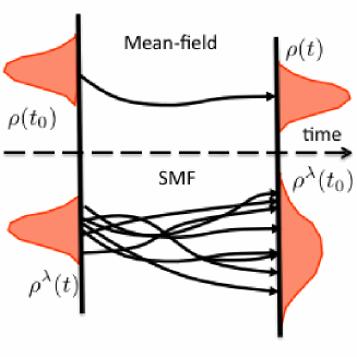
Figure 1: Illustration of the quantal mean-field approach (top) where a single density is propagated and of the SMF approach (bottom) where a set of densities are chosen and where each initial density is propagated independently from the others.

III From densities to observables: Ehrenfest formulation of the Stochastic Mean-Field Theory

The mean-field theory is a quantal approach and even if it usually underestimates fluctuations of collective observables in the nuclear physics context, these fluctuations are non-zero. Within mean-field theory, the expectation value of an observable $\hat{O}$ is obtained through $\langle\hat{O}\rangle={\rm Tr}(\hat{O}\hat{D})$ where $\hat{D}$ has the form (3). Accordingly, the quantal average and fluctuations of a one-body observable $\hat{Q}$ along the mean-field trajectory are given by:

$$\langle\hat{Q}\rangle=\sum_{i}\langle\varphi_{i}(t)|\hat{Q}|\varphi_{i}(t)\rangle n_{i}$$ (9)

and

$$\sigma^{2}_{Q}(t)=\langle\hat{Q}^{2}\rangle-\langle\hat{Q}\rangle^{2}=\sum_{i}|\langle\varphi_{i}(t)|\hat{Q}|\varphi_{i}(t)\rangle|^{2}n_{i}(1-n_{i}).$$ (10)

An important aspect of the SMF approach is that the quantum expectation value is replaced by a classical statistical average over the initial conditions. Denoting by $Q^{\lambda}(t)$ the value of the observable at time $t$ for a given event, fluctuations are obtained using

$$\sigma^{2}_{\rm SMF}(t) = \overline{(Q^{\lambda}(t)-Q(t))^{2}}$$ (11)

where $Q(t)=\overline{Q^{\lambda}(t)}$. The statistical properties of initial conditions insures that quantal fluctuations [$\sigma^{2}_{Q}$] and statistical [$\sigma^{2}_{\rm SMF}$] fluctuations are equal at initial time. Note that such a classical mapping is a known technique to simulate quantum objects and might even be exact in some cases Her84 ; Kay94 .

In practice, it might be advantageous to select few collective degrees of freedom instead of the full one-body density matrix. At the mean-field level, the evolution of a set of one-body observable $\hat{Q}_{i}$ is given by the Ehrenfest theorem:

$$i\hbar\frac{d}{dt}\langle\hat{Q}_{i}\rangle=\langle[\hat{Q}_{i},\hat{H}]\rangle$$ (12)

If a complete set of one-body observables is taken, for instance if we consider full set of operators$\{a^{\dagger}_{i}a_{j}\}$, one recovers eq. (1). In many situations, one might further reduce the evolution to a restricted set of relevant degrees of freedoms in such a way that the mean-field approximation leads to a closed set of equations between them, i.e.

$$i\hbar\frac{d}{dt}\langle\hat{Q}_{i}\rangle={\cal F}\left(\langle\hat{Q}_{1}\rangle,\cdots,\langle\hat{Q}_{n}\rangle\right).$$ (13)

Starting from this equation, one can also formulate the SMF theory directly in the selected space of degrees of freedom by considering a set of initial conditions $\{Q^{\lambda}_{i}(t_{0})\}_{i=1,n}$ and by using directly the evolution:

$$i\hbar\frac{d}{dt}\hat{Q}^{\lambda}_{i}(t)={\cal F}\left(\hat{Q}^{\lambda}_{1}(t),\cdots,\hat{Q}^{\lambda}_{n}(t)\right).$$ (14)

for each initial condition $\lambda$. Note that statistical properties, i.e. first and second moments, of initial conditions should be computed using the conditions (6) and (7).

IV Illustrations

In recent years, we have applied the SMF approach either to schematic models or to realistic situations encountered in nuclear reactions where mean-field alone was unable to provide a suitable answer. Some examples are briefly discussed below.

IV.1 Many-body dynamics near a saddle point

As mentioned in the introduction, the mean-field theory alone cannot break a symmetry by itself. The symmetry breaking can often be regarded as the presence of a saddle point in a collective space while the absence of symmetry breaking in mean-field just means that the system will stay at the top of the saddle if it is left here initially. Such situation is well illustrated in the Lipkin-Meshkov-Glick model. This model consists of $N$ particles distributed in two N-fold degenerated single-particle states separated by an energy $\varepsilon$. The associated Hamiltonian is given by (taking $\hbar=1$),

$$H=\varepsilon J_{z}-V(J^{2}_{x}-J_{y}^{2}),$$ (15)

where $V$ denotes the interaction strength while $J_{i}$ ($i=x$, $y$, $z$), are the quasi-spin operators defined as

$$J_{z} = \frac{1}{2}\sum_{p=1}^{N}\left(c^{\dagger}_{+,p}c_{+,p}-c^{\dagger}_{-,p}c_{-,p}\right),$$

$$J_{x} = \frac{1}{2}(J_{+}+J_{-}),~{}~{}~{}J_{y}=\frac{1}{2i}(J_{+}-J_{-})$$ (16)

with $J_{+}=\sum_{p=1}^{N}c^{\dagger}_{+,p}c_{-,p}$, $J_{-}=J_{+}^{\dagger}$ and where $c^{\dagger}_{+,p}$ and $c^{\dagger}_{-,p}$ are creation operators associated with the upper and lower single-particle levels. In the following, energies and times are given in $\varepsilon$ and $\hbar/\varepsilon$ units respectively.

It could be shown that the TDHF dynamic can be recast as a set of coupled equations between the expectation values of the quasi-spin operators $j_{i}\equiv\langle J_{i}\rangle/N$ (for $i=x$, $y$ and $z$) given by:

$$\frac{d}{dt}\left(\begin{array}[]{c}j_{x}\\ j_{y}\\ j_{z}\end{array}\right) = \varepsilon\left(\begin{array}[]{ccc}0&-1+\chi j_{z}&\chi j_{y}\\ 1+\chi j_{z}&0&\chi j_{x}\\ -2\chi j_{y}&-2\chi j_{x}&0\end{array}\right)\left(\begin{array}[]{c}j_{x}\\ j_{y}\\ j_{z}\end{array}\right)$$ (26)

where $\chi=V(N-1)/\varepsilon$. Note that, this equation of motion is nothing but a special case of eq. (13) where the information is contained in the three quasi-spin components. To illustrate the symmetry breaking in this model it is convenient to display the Hartree-Fock energy ${\cal E}_{\rm HF}$ as a function of the $j_{z}$ component (Fig. 2). Note that, here the order parameter $\alpha=\frac{1}{2}{\rm acos}(-j_{z}/2)$ is used for conveniency. When the strength parameter is larger than a critical value ($\chi>1$), the parity symmetry is broken in $\alpha$ direction.

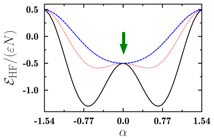
Figure 2: (color online). Evolution of the Hartree-Fock energy ${\cal E}_{\rm HF}$ as a function of $\alpha$ for $\chi=0.5$ (dashed line), $\chi=1.8$ (doted line) and $\chi=5$ (solid line) for $N=40$ particles. The arrow indicates the initial condition used in the SMF dynamics.

For $\chi>1$, if the system is initially at the position indicated by the arrow in Fig. 2, with TDHF it will remain at this point, i.e. this initial condition is a stationary solution of Eq. (26).

Following the strategy discussed above, a SMF approach can be directly formulated in collective space where initial random conditions for the spin components are taken. Starting from the statistical properties (6) and (7), it could be shown that the quasi-spins should be initially sampled according to Gaussian probabilities with first moments given by Lac12 :

$$\overline{j^{\lambda}_{x}(t_{0})}=\overline{j^{\lambda}_{y}(t_{0})}=0,$$ (27)

and second moments determined by,

$$\overline{j^{\lambda}_{x}(t_{0})j^{\lambda}_{x}(t_{0})}=\overline{j^{\lambda}_{y}(t_{0})j^{\lambda}_{y}(t_{0})}=\frac{1}{4N}.$$ (28)

while the $z$ component is a non fluctuating quantity.

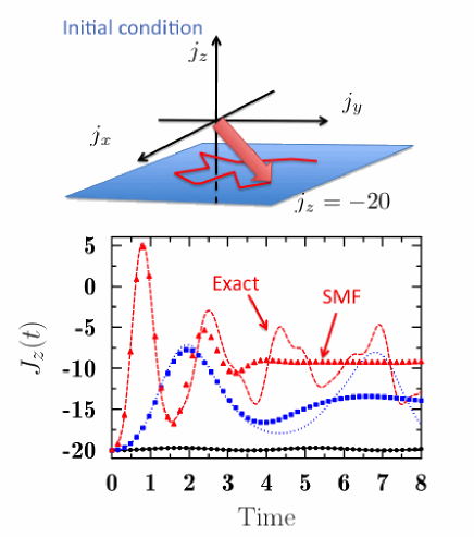
Figure 3: (color online) Top: illustration of the initial sampling used for the SMF theory in the collective space of quasi-spins. Bottom: Exact evolution of the $z$ quasi-spin component obtained when the initial state is $|j,-j\rangle$ for three different values of $\chi$: $\chi=0.5$ (solid line), $\chi=1.8$ (dotted line) and $\chi=5.0$ (dashed line) for $N=40$ particles. The corresponding results obtained with the SMF simulations are shown with circles, squares and triangles respectively. (adapted from Lac12 )

An illustration of the initial sampling (top) and of results obtained by averaging mean-field trajectories with different initial conditions is shown in Fig. 3 and compared to the exact dynamic. As we can see from the figure, while the original mean-field gives constant quasi-spins as a function of time, the SMF approach greatly improves the dynamics and follows the exact evolution up to a certain time that depends on the interaction strength. As shown in Fig. 4, the stochastic approach not only improves the description of the mean-value of one-body observables but also the fluctuations.

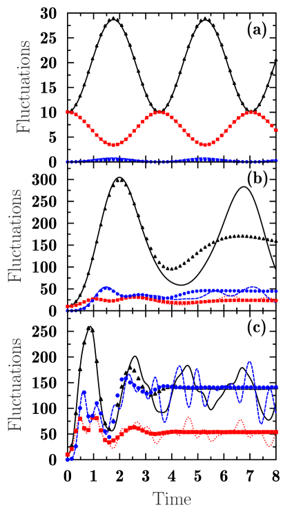
Figure 4: (color online) Exact evolution of dispersions of quasi-spin operators obtained when the initial state is $|j,-j\rangle$ for three different values of $\chi$, from top to bottom $\chi=0.5$ (a), $\chi=1.8$ (b) and $\chi=5.0$ (c) are shown. In each case, solid, dashed and dotted lines correspond to $\sigma^{2}_{x}(t)$, $\sigma^{2}_{y}(t)$ and $\Delta^{2}_{z}(t)$, respectively. In each case, results of the SMF simulations are shown with triangles ($\sigma^{2}_{x}$), squares ($\sigma^{2}_{y}$) and circles ($\sigma^{2}_{z}$). (taken from Lac12 )

V Application to nuclear reactions

The SMF has been recently used to deduce transport coefficients associated to momentum dissipation or mass transfer during reactions from a fully microscopic theory Ayi09 ; Was09 ; Yil11 . The TDHF theory provides a powerful way to get insight nuclear reaction and treat various effects like deformation, nucleon transfer, fusion, … in a quantal transport theory. An illustration of nuclear densities obtained at various time of the ⁴⁰Ca + ⁹⁰Zr reactions is given in Fig. 5.

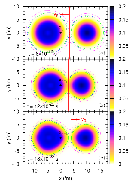
Figure 5: (color online). Snapshots of the nucleon density profiles on the reaction plane, $\rho(x,y,z=0)$, are indicated by contour plots for the central collision of ⁴⁰Ca + ⁹⁰Zr system at $E_{\rm cm}=97$ MeV in units of fm^-3. The black dot is the center of mass point. The red lines indicate the positions of the window $x_{0}$ and $v_{0}=dx_{0}/dt$ denotes velocity of the window. (taken from Yil11 )

The mean-field approach does include the so-called one-body dissipation associated to the deformation of the system and/or to the exchange of particles. For instance, considering a set of observables, denoted generically $\mathbf{Q}\equiv\{\hat{Q}_{i}\}$, like the relative distance, relative momentum, angular momentum between nuclei or the number of nucleons inside one of the nucleus, it is possible to reduce the TDHF evolution and obtain classical equations of motion of the form:

$$\frac{\partial Q_{i}}{\partial t} = F(\mathbf{Q},t)-\sum_{j}\nu_{ij}(\mathbf{Q},t)Q_{j},$$ (29)

where $F$ is an eventual driving force while $\nu$ corresponds to drift coefficients. For instance, the nucleus-nucleus interaction potential and energy loss associated to internal dissipation has been extracted in ref. Was08 ; Was09 using such formula.

When TDHF is extended to incorporate initial fluctuations, the equation of motion itself becomes a stochastic process:

$$\frac{\partial Q^{\lambda}_{i}}{\partial t} = F(\mathbf{Q^{\lambda}},t)-\sum_{j}\nu_{ij}(\mathbf{Q^{\lambda}},t)Q^{\lambda}_{j}+\delta Q^{\lambda}_{i}.$$ (30)

For short time, the average drifts $\bar{\nu}_{ij}$ should identify with the TDHF one while the extra term is a random variables that leads to dispersion around the mean trajectory. In the Markov limit, one can define the diffusion coefficient

$$\overline{\delta Q^{\lambda}_{i}(t)\delta Q^{\lambda}_{j}(t)} = 2\delta(t-t^{\prime})D_{ij}(t).$$ (31)

This mapping has been recently used to not only study dissipative process but also estimate fluctuations properties in the momentum and mass exchange. Denoting by $D_{AA}(t)$ the diffusion coefficient associated with mass, fluctuations in mass of the target and/or projectile can be computed using the simple formula

$$\sigma^{2}_{AA}(t)\simeq 2\int_{0}^{t}D_{AA}(s)ds.$$ (32)

In figure 6, an example of estimated variances during the asymmetric reaction ⁴⁰Ca + ⁹⁰Zr is shown as a function of time in the case of fusion reaction (top) or below the Coulomb barrier (middle and bottom panel).

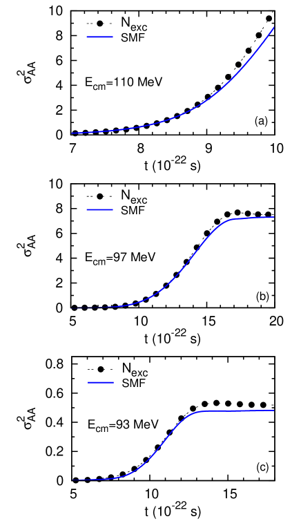
Figure 6: Variances of fragment mass distributions are plotted versus time in collisions of ⁴⁰Ca + ⁹⁰Zr system at three different center-of-mass energies. The dotted lines denote total number of exchanged nucleons until a given time $t$. (taken from Yil11 )

All cases correspond to central collisions. Note that below the Coulomb barrier the target and projectile re-separate after having exchanged few nucleons corresponding to transfer reactions. In general, it is observed that the fluctuations are greatly increased compared to the original TDHF and are compatible with the net number of exchanged nucleons from one nucleus to the other (dotted line in Fig. 6).

VI Summary

In this contribution, illustrations of the application of the stochastic mean-field theory are discussed. It is shown, that the introduction of initial fluctuations followed by a set of independent mean-field trajectories greatly improves the original mean-field picture. In particular, it seems that this approach is a powerful to increase the fluctuations that are generally strongly underestimated in TDHF or to describe the many-body dynamics close to a saddle point.

Acknowledgments S.A., B.Y., and K.W. gratefully acknowledge GANIL for the support and warm hospitality extended to them during their visits. This work is supported in part by the US DOE Grant No. DE-FG05-89ER40530.

References

- (1) D. Lacroix, S. Ayik, and Ph. Chomaz, Prog. Part. Nucl. Phys. 52, (2004) 497.
- (2) S. Ayik, Phys. Lett. B 658, (2008) 174.
- (3) D. Lacroix, S. Ayik and B. Yilmaz, Phys. Rev. C85, (2012) 041602
- (4) S. Ayik, K. Washiyama, and D. Lacroix, Phys. Rev. C 79, (2009) 054606.
- (5) K. Washiyama, S. Ayik, and D. Lacroix, Phys. Rev. C 80, (2009) 031602(R).
- (6) B. Yilmaz, S. Ayik, D. Lacroix and K. Washiyama, Phys. Rev. C83, (2011) 064615.
- (7) C. Simenel, B. Avez, and D. Lacroix, in Lecture notes of the International Joliot-Curie School,Maubuisson, (2007), arXiv:0806.2714.
- (8) J. P. Blaizot and G. Ripka, Quantum Theory of Finite Systems, (MIT Press, Cambridge, Massachusetts, 1986).
- (9) P. Ring and P. Schuck, The Nuclear Many-Body Problem (Springer-Verlag, New-York, 1980).
- (10) M. F. Herman and E. Kluk, Chem. Phys. 91, 27 (1984).
- (11) K. G. Kay, J. Chem. Phys. 100, 4432 (1994); 101, 2250 (1994).
- (12) K. Washiyama and D. Lacroix, Phys. Rev. C 78, 024610 (2008).