Darboux transformation and positons of the inhomogeneous Hirota and the Maxwell-Bloch equation

Abstract.

In this paper, we derive Darboux transformation of the inhomogeneous Hirota and the Maxwell-Bloch(IH-MB) equations which is governed by femtosecond pulse propagation through inhomogeneous doped fibre. The determinant representation of Darboux transformation is used to derive soliton solutions, positon solutions of the IH-MB equations.

PACS numbers: 42.65.Tg, 42.65.Sf, 05.45.Yv, 02.30.Ik.
Keywords: the inhomogeneous Hirota and Maxwell-Bloch equations, Darboux transformation, soliton solution, positon solution.

1. Introduction

In recent years, nonlinear science has emerged as a powerful subject for explaining the mystery present in the challenges of science and technology today. Among nonlinear science, the interplay between dispersion and nonlinearity gives rise to several important phenomena in optical fibers, including parametric amplification, wavelength conversion, modulational instability(MI), soliton propagation and so on. Among all concepts, solitons, positons and rogons have been not only the subject of intensive research in oceanography[1, 2] but also it has been studied extensively in several areas, such as Bose-Einstein condensate, plasma, superfluid, finance, optics and so on [3, 4, 5, 6, 7, 8, 9].

An important ingredient in the development of the theory of soliton and of complete integrability has been the interplay between mathematics and physics. In 1973, Hasegawa and Tappert [10] modeled the propagation of coherent optical pulses in optical fibres by nonlinear Schrödinger (NLS) equation without the inclusion of fibre loss. They showed theoretically that generation and propagation of shape-preserving pulses called solitons in optical fibres is possible by balancing the dispersion and nonlinearity.

In 1967, McCall and Hahn [11] had explained a special type of lossless pulse propagation in two-level resonant media. They have discovered the self-induced transparency(SIT) which can be explained by Maxwell-Bloch(MB) equations. The coherent absorption takes place and the media becomes optically transparent to that particular wavelength when the energy difference between the two levels of the media coincide with the optical wavelength. Burtsev and Gabitov[12] have considered MB equations with pumping and damping which is useful in optical pumping during the propagation of optical pulses in resonant atoms, and in their paper the Lax pair was presented for deformed MB systems.

The important constraint to the NLS soliton namely the optical losses can be somewhat compensated with the effect of SIT. Therefore the system will be governed by the coupled system of the NLS equation and the MB equation (NLS-MB equations) if we consider these effects for a large width pulse. The coexistence of NLS solitons and SIT solitons in erbium-doped resonant fibres was experimentally observed by Nakazawa et al [13, 14]. Recently, multi-soliton solutions of coupled NLS-MB equation was shown in [15]. In [16], the periodic solutions have been generated through Darboux transformation and later rogue wave solutions were derived from breather solution in [17]. Modeling photonic crystal fiber for efficient soliton pulse propagation at 850 nm was surveyed in [18]. It presents new types of Dark-in-the-Bright solutions also called dipole soliton for the higher order nonlinear NLS (HNLS) equation with non-Kerr nonlinearity under some parametric conditions and subject to constraint relation among the parameters in optical context in [19]. Impact of fourth-order dispersion in the modulational instability spectra of wave propagation in glass fibers with saturable nonlinearity was considered in [20]. The HNLS-MB equations as a higher-order correction of NLS-MB equations were shown that they allow soliton-type pulse propagation under a particular parametric condition[21, 22].

For a reduced dynamical equation, the erbium-doped fibre system was proven to allow soliton-type pulse propagation with pumping[23]. The Lax pair and the exact soliton solution for Higher-order nonlinear Schrödinger and Maxwell-Bloch(HNLS-MB) equations with pumping was derived in [23].

Kodama[24] has shown that with suitable transformation and omitting the higher-order terms, higher order Nonlinear Schrödinger equation equation can be reduced to the Hirota equation[25]whose rogue wave solution is already reported in [26, 27]. In a similar way,after suitable choice of self steepening and self frequency effects, the HNLS-MB equations can be reduced to a coupled system of the Hirota equation and MB equation[28]. The H-MB equations can be seen as the higher order correction of the NLS-MB equations and is the coupled system of the Hirota equation and the MB equation[31]. The H-MB system has been shown to be integrable and also admits the Lax pair and other required properties for complete integrability [28].

It is well known that the Darboux transformation is an efficient method to generate the soliton solutions for integrable equations[29, 37]. The determinant representation of n-fold Darboux transformation of AKNS system was given in [30]. In [31], it constructed n-folds Darboux transformation of the H-MB equations, meanwhile the rogue wave solutions of the H-MB equations were obtained using the Darboux transformation.

Inhomogeneous integrable equations become more and more attractive[32]. Recently, K. Porsezian and C. G. Latchio Tiofack, Thierry B. Ekogo, etal. consider dynamics of bright solitons and their collisions for the inhomogeneous coupled nonlinear Schrödinger-Maxwell-Bloch equations which describes propagation of an optical soliton in an inhomogeneous nonlinear waveguide doped with two level resonant atoms[33]. Soliton interactions in a generalized inhomogeneous Hirota-Maxwell-Bloch(IH-MB) system were considered in [38, 34] with symbolic computation but positon solutions of IH-MB is still unknown.

The purpose of this paper is to derive the determinant representation of Darboux transformation which is used to derive soliton solutions, positon solutions of the IH-MB equations.

The paper is organized as follows. In Section 2, the Lax representation of IH-MB equations will be introduced firstly. In Section 3, we derived the one-fold Darboux transformation of the H-MB equations. In Section 4, the determinant-formed generalization of one-fold Darboux transformation to 2-fold Darboux transformation of the IH-MB equations will be given. Using these Darboux transformations, one soliton, two soliton and positons are derived in Section 5 and Section 6 by assuming trivial seed solutions. Section 7 is devoted to conclusion and discussions.

2. Lax representation of the IH-MB system

In this paper, we will concentrate on the inhomogeneous Hirota and the Maxwell-Bloch(H-MB) system as following specific form[34, 38],

$$E_{z} = -(a_{1}(z)E_{t}+a_{2}(z)E+ia_{3}(z)E_{tt}+a_{4}(z)E_{ttt}+a_{5}(z)|E|^{2}E_{t}$$

$$+ia_{6}(z)|E|^{2}E+a_{7}(z)p),$$

$$p_{t} = 2b_{1}(z)E\eta-2ib_{2}(z)\omega p,$$ (2.2)

$$\eta_{t} = -b_{1}(z)(Ep^{*}+E^{*}p),$$ (2.3)

with constraint

$$a_{2}=\frac{\frac{\partial b_{1}}{\partial z}}{b_{1}};a_{5}=6a_{4}b_{1}^{2};a_{6}=2a_{3}b_{1}^{2}.$$ (2.4)

In the equations above, $z$ and $t$ represent the normalized distance and time respectively, $E(z,t)$ denotes the slowly varying envelope axial field, $p(z,t)$ is the measure of the polarization of the resonant medium, and $\eta(z,t)$ represents the extent of the population inversion. $a_{1}(z)$ results from the group velocity and $a_{2}(z)$ describes the amplification or absorption. The coefficients $a_{3}(z)\sim a_{6}(z)$ represent the group velocity dispersion (GVD), the third-order dispersion(TOD)[35], self-steepening (SS)[36], and self-phase modulation respectively. $a_{7}(z)$ is the parameter describing the averaging with respect to inhomogeneous broadening of the resonant frequency. $b_{1}(z)$ and $b_{2}(z)$ depict the character of interactions between the propagation field and the erbium atoms. The real parameter $\omega$ is a constant corresponding to the frequency, and the $*$ denotes the complex conjugate. If we set

$$a_{1}=a_{2}=0,a_{3}=-\frac{1}{2}\alpha,a_{4}=-\beta,a_{5}=-6\beta,a_{6}=-\alpha,a_{7}=-2,b_{1}=1,b_{2}=-1,$$ (2.5)

the inhomogeneous H-MB equation will be reduced to H-MB equation as following

$$E_{z} = i\alpha(\frac{1}{2}E_{tt}+|E|^{2}E)+\beta(E_{ttt}+6|E|^{2}E_{t})+2p,$$ (2.6)

$$p_{t} = 2i\omega p+2E\eta,$$ (2.7)

$$\eta_{t} = -(Ep^{*}+E^{*}p).$$ (2.8)

We will call the inhomogeneous Hirota and the Maxwell-Bloch system when $\alpha=2,\beta=-1$ the classical H-MB equation. The linear eigenvalue problem of IH-MB takes the form

$$\Phi_{t} = U\Phi,$$ (2.9)

$$\Phi_{z} = V\Phi,$$ (2.10)

where $U$ and $V$ can be expressed in following polynomials about complex constant eigenvalue parameter $\lambda$

$$U = \lambda\left(\begin{matrix}1&0\\ 0&-1\end{matrix}\right)+\left(\begin{matrix}0&b_{1}(z)E\\ -b_{1}(z)E^{*}&0\end{matrix}\right)=\lambda\sigma_{3}+U_{0},$$ (2.11)

$$V = \lambda^{3}\left(\begin{matrix}-4a_{4}&0\\ 0&4a_{4}\end{matrix}\right)+\lambda^{2}\left(\begin{matrix}-2ia_{3}&-4a_{4}b_{1}E\\ 4a_{4}b_{1}E^{*}&2ia_{3}\end{matrix}\right)+\lambda\left(\begin{matrix}-a_{1}-2a_{4}b_{1}^{2}|E|^{2}&-2ib_{1}(a_{3}E-ia_{4}E_{t})\\ 2ia_{3}b_{1}E^{*}-2a_{4}b_{1}E_{t}^{*}&a_{1}+2a_{4}b_{1}^{2}|E|^{2}\end{matrix}\right)$$ (2.12)

$$+\left(\begin{matrix}-C_{1}&-b_{1}B_{1}\\ -b_{1}B_{1}^{*}&C_{1}\end{matrix}\right)+A_{1}\left(\begin{matrix}\eta&-p\\ -p^{*}&-\eta\end{matrix}\right)$$

$$= \lambda^{3}V_{3}+\lambda^{2}V_{2}+\lambda V_{1}+V_{0}+\frac{1}{\lambda+i\omega b_{2}}V_{-1},$$

where

$$V_{-1}=-\frac{b_{1}a_{7}}{2}\left(\begin{matrix}\eta&-p\\ -p^{*}&-\eta\end{matrix}\right),$$ (2.13)

$$A_{1}=-\frac{b_{1}a_{7}}{2(\lambda+i\omega b_{2})},\ \ B_{1}:=2a_{4}b_{1}^{2}E^{*}E^{2}+a_{1}E+ia_{3}E_{t}+a_{4}E_{tt},$$ (2.14)

$$C_{1}:=ia_{3}b_{1}^{2}EE^{*}+a_{4}b_{1}^{2}(E^{*}E_{t}-EE_{t}^{*}).$$ (2.15)

$V_{i}$ denotes the coefficient matrix of term $\lambda^{i}$ and

$$\Phi = \Phi(\lambda)=\left(\begin{matrix}\Phi_{1}(\lambda,t,z)\\ \Phi_{2}(\lambda,t,z)\end{matrix}\right)$$ (2.16)

is an eigenfunction associated with eigenvalue parameter $\lambda$ of linear system eq.(2.9-2.10).

Using the linear equations of H-MB equations, One-fold Daroux transformation for IH-MB equation will be introduced in the next section.

3. One-fold Daroux transformation for the IH-MB equation

In this section, we will give the detailed proof of the one-fold Daroux transformation for the IH-MB equation. Firstly, we consider the transformation about linear function $\Phi$

$$\Phi^{\prime} = T\Phi=(\lambda A-S)\Phi,$$ (3.1)

where

$$A=\left(\begin{matrix}a_{11}&a_{12}\\ a_{21}&a_{22}\end{matrix}\right),\ \ \ S=\left(\begin{matrix}s_{11}&s_{12}\\ s_{21}&s_{22}\end{matrix}\right).$$ (3.2)

New function $\Phi^{\prime}$ is supposed to satisfy

$$\Phi^{\prime}_{t} = U^{\prime}\Phi^{\prime},$$ (3.3)

$$\Phi^{\prime}_{z} = V^{\prime}\Phi^{\prime}.$$ (3.4)

Then matrix $T$ can be proven to satisfy following identities

$$T_{t}+TU = U^{\prime}T,$$ (3.5)

$$T_{z}+TV = V^{\prime}T.$$ (3.6)

Bring the form of matrices $A$ and $S$ into eq.(3.5) and comparing the coefficients of both sides will lead to following condition

$$a_{12}=a_{21}=0,\ \ \ (a_{11})_{t}=(a_{22})_{t}=0.$$ (3.7)

Therefore we will choose $A=I$ and $T=\lambda I-S$ in the following part of this paper. The relation between $E,p,\eta$ and new solutions $E^{\prime},p^{\prime},\eta^{\prime}$ which is called Darboux transformation can be got by eq. (3.5) and eq. (3.6).

From (3.5), we have

$$E^{\prime} = E+2b_{1}^{-1}s_{12},$$ (3.8)

$$S_{t} = \left(\begin{matrix}0&b_{1}E\\ -b_{1}E^{*}&0\end{matrix}\right)S-S\left(\begin{matrix}0&b_{1}E\\ -b_{1}E^{*}&0\end{matrix}\right)-[S,\sigma_{3}]S,$$ (3.9)

and $S$ should have a condition as $s_{21}=s^{*}_{12}.$ By (3.6), following identity can be got

$$-S_{z}+(\lambda I-S)(\lambda^{3}V_{3}+\lambda^{2}V_{2}+\lambda V_{1}+V_{0}+\frac{1}{\lambda+i\omega b_{2}}V_{-1})$$ (3.10)

$$= (\lambda^{3}V_{3}+\lambda^{2}V^{\prime}_{2}+\lambda V^{\prime}_{1}+V^{\prime}_{0}+\frac{1}{\lambda+i\omega b_{2}}V^{\prime}_{-1})(\lambda I-S).$$ (3.11)

Multiplying both sides of eq.(3.10) by $\lambda I-S$ can lead to

$$-S_{z}(\lambda+i\omega b_{2})+(\lambda I-S)(\lambda^{3}(\lambda+i\omega b_{2})V_{3}+\lambda^{2}(\lambda+i\omega b_{2})V_{2}+\lambda(\lambda+i\omega b_{2})V_{1}+V_{0}(\lambda+i\omega b_{2})+V_{-1})$$

$$= (\lambda^{3}(\lambda+i\omega b_{2})V_{3}+\lambda^{2}(\lambda+i\omega b_{2})V^{\prime}_{2}+\lambda(\lambda+i\omega b_{2})V^{\prime}_{1}+V^{\prime}_{0}(\lambda+i\omega b_{2})+V^{\prime}_{-1})(\lambda I-S).$$

For term with $\lambda^{0}$, we get following identity

$$S_{z}i\omega b_{2}+S(i\omega b_{2}V_{0}+V_{-1})=(i\omega b_{2}V^{\prime}_{0}+V^{\prime}_{-1})S,$$

which further leads to

$$S_{z} = (V^{\prime}_{0}-i\omega^{-1}b_{2}^{-1}V^{\prime}_{-1})S-S(-i\omega^{-1}b_{2}^{-1}V_{-1}+V_{0}).$$

For term with $\lambda$, we get following identity

$$S_{z} = (i\omega b_{2}V_{0}+V_{-1})-S(i\omega b_{2}V_{1}+V_{0})+(i\omega b_{2}V^{\prime}_{1}+V^{\prime}_{0})S+(-i\omega b_{2}V^{\prime}_{0}-V^{\prime}_{-1}).$$

For term with $\lambda^{2}$, we get following identity

$$(i\omega b_{2}V_{1}+V_{0})-S(i\omega b_{2}V_{2}+V_{1}) = (i\omega b_{2}V^{\prime}_{1}+V^{\prime}_{0})-(i\omega b_{2}V^{\prime}_{2}+V^{\prime}_{1})S.$$

For term with $\lambda^{3}$, we get following identity

$$(i\omega b_{2}V_{2}+V_{1})-S(i\omega b_{2}V_{3}+V_{2}) = (i\omega b_{2}V^{\prime}_{2}+V^{\prime}_{1})-(i\omega b_{2}V_{3}+V^{\prime}_{2})S.$$

For term with $\lambda^{4}$, we get following identity

$$V^{\prime}_{2}=V_{2}-[S,V_{3}],$$

From above several identities, we can get

$$E^{\prime} = E+2b_{1}^{-1}s_{12},$$ (3.12)

$$V^{\prime}_{-1}=(S+i\omega b_{2})V_{-1}(S+i\omega b_{2})^{-1},$$ (3.13)

which gives one fold transformation of one-fold Darboux transformation of H-MB equations.

Suppose

$$S=H\Lambda H^{-1}$$ (3.14)

where $\Lambda=\left(\begin{matrix}\lambda_{1}&0\\ 0&\lambda_{2}\end{matrix}\right)$, $H=\left(\begin{matrix}\Phi_{1}(\lambda_{1},t,z)&\Phi_{1}(\lambda_{2},t,z)\\ \Phi_{2}(\lambda_{1},t,z)&\Phi_{2}(\lambda_{2},t,z)\end{matrix}\right):=\left(\begin{matrix}\Phi_{1,1}&\Phi_{1,2}\\ \Phi_{2,1}&\Phi_{2,2}\end{matrix}\right).$

In order to satisfy the constraints of $S$ and make $V^{\prime}_{-1}$ having similar form as $V_{-1}$, i.e. $s_{21}=s^{*}_{12},$ following constraint will be considered

$$\lambda_{2} = -\lambda_{1}^{*},\ \ s_{11}=-s^{*}_{22},$$ (3.15)

$$H = \left(\begin{matrix}\Phi_{1}(\lambda_{1},t,z)&-\Phi^{*}_{2}(\lambda_{1},t,z)\\ \Phi_{2}(\lambda_{1},t,z)&\Phi^{*}_{1}(\lambda_{1},t,z)\end{matrix}\right).$$ (3.16)

The detailed determinant form of one-fold Darboux transformation of IH-MB equations in form of eigenfunctions will be given in the next section.

4. Determinant representation of Darboux transformation

In this section, we will give determinant representation of the first two Darboux transformation of the IH-MB equations. Other higher-order Darboux transformation can be got in similar way which can be seen clearly in our paper [31]. Firstly, we introduce n eigenfunctions $\left(\begin{matrix}\Phi_{1,i}\\ \Phi_{2,i}\end{matrix}\right)=\Phi(\lambda=\lambda_{i}),i=1,2$ with constraints on eigenvalues as $\lambda_{2i-1}=-\lambda_{2i}^{*}$ and the reduction conditions on eigenfunctions as $\Phi_{2,2i}=\Phi_{1,2i-1}^{*},\ \ \Phi_{2,2i-1}=-\Phi_{1,2i}^{*}$.

As the simplest Darboux transformation, the determinant representation of one-fold Darboux transformation of the IH-MB equations will be given in the following theorem.

Theorem 4.1.

The one-fold Darboux transformation of the IH-MB equations is as following

$$T_{1}(\lambda,\lambda_{1},\lambda_{2})=\lambda I+t_{0}^{[1]}=\frac{1}{\Delta_{1}}\left(\begin{matrix}(\mathbb{T}_{1})_{11}&(\mathbb{T}_{1})_{12}\\ (\mathbb{T}_{1})_{21}&(\mathbb{T}_{1})_{22}\end{matrix}\right)$$ (4.1)

where

$$t_{0}^{[1]}=\frac{1}{\Delta_{1}}\left(\begin{matrix}\left|\begin{matrix}\Phi_{2,1}&\lambda_{1}\Phi_{1,1}\\ \Phi_{2,2}&\lambda_{2}\Phi_{1,2}\end{matrix}\right|&-\left|\begin{matrix}\Phi_{1,1}&\lambda_{1}\Phi_{1,1}\\ \Phi_{1,2}&\lambda_{2}\Phi_{1,2}\end{matrix}\right|\\ \\ \left|\begin{matrix}\Phi_{2,1}&\lambda_{1}\Phi_{2,1}\\ \Phi_{2,2}&\lambda_{2}\Phi_{2,2}\end{matrix}\right|&-\left|\begin{matrix}\Phi_{1,1}&\lambda_{1}\Phi_{2,1}\\ \Phi_{1,2}&\lambda_{2}\Phi_{2,2}\end{matrix}\right|\end{matrix}\right),\ \ \Delta_{1}=\left|\begin{matrix}\Phi_{1,1}&\Phi_{2,1}\\ \Phi_{1,2}&\Phi_{2,2}\end{matrix}\right|,$$ (4.2)

$$(\mathbb{T}_{1})_{11} = \left|\begin{matrix}1&0&\lambda\\ \Phi_{1,1}&\Phi_{2,1}&\lambda_{1}\Phi_{1,1}\\ \Phi_{1,2}&\Phi_{2,2}&\lambda_{2}\Phi_{1,2}\ \end{matrix}\right|,\ \ (\mathbb{T}_{1})_{12}=\left|\begin{matrix}0&1&0\\ \Phi_{1,1}&\Phi_{2,1}&\lambda_{1}\Phi_{1,1}\\ \Phi_{1,2}&\Phi_{2,2}&\lambda_{2}\Phi_{1,2}\end{matrix}\right|,$$ (4.3)

$$(\mathbb{T}_{1})_{21} = \left|\begin{matrix}1&0&0\\ \Phi_{1,1}&\Phi_{2,1}&\lambda_{1}\Phi_{2,1}\\ \Phi_{1,2}&\Phi_{2,2}&\lambda_{2}\Phi_{2,2}\end{matrix}\right|,\ \ (\mathbb{T}_{1})_{22}=\left|\begin{matrix}0&1&\lambda\\ \Phi_{1,1}&\Phi_{2,1}&\lambda_{1}\Phi_{2,1}\\ \Phi_{1,2}&\Phi_{2,2}&\lambda_{2}\Phi_{2,2}\end{matrix}\right|,$$ (4.4)

and

$$U^{[1]}=U+[T_{1},\sigma_{3}],\ \ V^{[1]}_{-1}=T_{1}|_{\lambda=-i\omega b_{2}}V_{-1}T_{1}^{-1}|_{\lambda=-i\omega b_{2}},$$ (4.5)

$$E^{[1]} = E+2b_{1}^{-1}s_{12}=E-2b_{1}^{-1}\frac{(T_{1})_{12}}{\Delta_{1}},$$ (4.6)

$$p^{[1]} = \frac{2\eta(T_{1})_{11}(T_{1})_{12}-p^{*}(T_{1})_{12}(T_{1})_{12}+p(T_{1})_{11}(T_{1})_{11}}{(T_{1})_{11}(T_{1})_{22}-(T_{1})_{12}(T_{1})_{21}}|_{\lambda=-i\omega b_{2}},$$ (4.7)

$$\eta^{[1]} = \frac{\eta((T_{1})_{11}(T_{1})_{22}+(T_{1})_{12}(T_{1})_{21})-p^{*}(T_{1})_{12}(T_{1})_{22}+p(T_{1})_{11}(T_{1})_{21}}{(T_{1})_{11}(T_{1})_{22}-(T_{1})_{12}(T_{1})_{21}}|_{\lambda=-i\omega b_{2}}.$$ (4.8)

We can find the transformation $T_{1}$ has following property

$$T_{1}(\lambda;\lambda_{1},\lambda_{2})|_{\lambda=\lambda_{i}}\left(\begin{matrix}\Phi_{1,i}\\ \Phi_{2,i}\end{matrix}\right)=0,$$ (4.9)

where $i=1,2.$

This one-fold transformation will be used to generate one-soliton solution from trivial seed solution of the IH-MB equation.

In the next part, we will generalize the Darboux transformation to two-fold case which is contained in the following theorem.

Theorem 4.2.

The two-fold Darboux transformation of H-MB equation is as following

$$T_{2}(\lambda;\lambda_{1},\lambda_{2},\lambda_{3},\lambda_{4})=\lambda^{2}I+t_{1}^{[2]}\lambda+t_{0}^{[2]}=\frac{1}{\Delta_{2}}\left(\begin{matrix}(\mathbb{T}_{2})_{11}&(\mathbb{T}_{2})_{12}\\ (\mathbb{T}_{2})_{21}&(\mathbb{T}_{2})_{22}\end{matrix}\right)$$ (4.10)

where

$$\Delta_{2} = \left|\begin{matrix}\Phi_{1,1}&\Phi_{2,1}&\lambda_{1}\Phi_{1,1}&\lambda_{1}\Phi_{2,1}\\ \Phi_{1,2}&\Phi_{2,2}&\lambda_{2}\Phi_{1,2}&\lambda_{2}\Phi_{2,2}\\ \Phi_{1,3}&\Phi_{2,3}&\lambda_{3}\Phi_{1,3}&\lambda_{3}\Phi_{2,3}\\ \Phi_{1,4}&\Phi_{2,4}&\lambda_{4}\Phi_{1,4}&\lambda_{4}\Phi_{2,4}\end{matrix}\right|,$$ (4.11)

$$(\mathbb{T}_{2})_{11} = \left|\begin{matrix}1&0&\lambda&0&\lambda^{2}\\ \Phi_{1,1}&\Phi_{2,1}&\lambda_{1}\Phi_{1,1}&\lambda_{1}\Phi_{2,1}&\lambda_{1}^{2}\Phi_{1,1}\\ \Phi_{1,2}&\Phi_{2,2}&\lambda_{2}\Phi_{1,2}&\lambda_{2}\Phi_{2,2}&\lambda_{2}^{2}\Phi_{1,2}\\ \Phi_{1,3}&\Phi_{2,3}&\lambda_{3}\Phi_{1,3}&\lambda_{3}\Phi_{2,3}&\lambda_{3}^{2}\Phi_{1,3}\\ \Phi_{1,4}&\Phi_{2,4}&\lambda_{4}\Phi_{1,4}&\lambda_{4}\Phi_{2,4}&\lambda_{4}^{2}\Phi_{1,4}\end{matrix}\right|,\ \ (\mathbb{T}_{2})_{12}=\left|\begin{matrix}0&1&0&\lambda&0\\ \Phi_{1,1}&\Phi_{2,1}&\lambda_{1}\Phi_{1,1}&\lambda_{1}\Phi_{2,1}&\lambda_{1}^{2}\Phi_{1,1}\\ \Phi_{1,2}&\Phi_{2,2}&\lambda_{2}\Phi_{1,2}&\lambda_{2}\Phi_{2,2}&\lambda_{2}^{2}\Phi_{1,2}\\ \Phi_{1,3}&\Phi_{2,3}&\lambda_{3}\Phi_{1,3}&\lambda_{3}\Phi_{2,3}&\lambda_{3}^{2}\Phi_{1,3}\\ \Phi_{1,4}&\Phi_{2,4}&\lambda_{4}\Phi_{1,4}&\lambda_{4}\Phi_{2,4}&\lambda_{4}^{2}\Phi_{1,4}\end{matrix}\right|,$$

$$(\mathbb{T}_{2})_{21} = \left|\begin{matrix}1&0&\lambda&0&0\\ \Phi_{1,1}&\Phi_{2,1}&\lambda_{1}\Phi_{1,1}&\lambda_{1}\Phi_{2,1}&\lambda_{1}^{2}\Phi_{2,1}\\ \Phi_{1,2}&\Phi_{2,2}&\lambda_{2}\Phi_{1,2}&\lambda_{2}\Phi_{2,2}&\lambda_{2}^{2}\Phi_{2,2}\\ \Phi_{1,3}&\Phi_{2,3}&\lambda_{3}\Phi_{1,3}&\lambda_{3}\Phi_{2,3}&\lambda_{3}^{2}\Phi_{2,3}\\ \Phi_{1,4}&\Phi_{2,4}&\lambda_{4}\Phi_{1,4}&\lambda_{4}\Phi_{2,4}&\lambda_{4}^{2}\Phi_{2,4}\end{matrix}\right|,\ \ (\mathbb{T}_{2})_{22}=\left|\begin{matrix}0&1&0&\lambda&\lambda^{2}\\ \Phi_{1,1}&\Phi_{2,1}&\lambda_{1}\Phi_{1,1}&\lambda_{1}\Phi_{2,1}&\lambda_{1}^{2}\Phi_{2,1}\\ \Phi_{1,2}&\Phi_{2,2}&\lambda_{2}\Phi_{1,2}&\lambda_{2}\Phi_{2,2}&\lambda_{2}^{2}\Phi_{2,2}\\ \Phi_{1,3}&\Phi_{2,3}&\lambda_{3}\Phi_{1,3}&\lambda_{3}\Phi_{2,3}&\lambda_{3}^{2}\Phi_{2,3}\\ \Phi_{1,4}&\Phi_{2,4}&\lambda_{4}\Phi_{1,4}&\lambda_{4}\Phi_{2,4}&\lambda_{4}^{2}\Phi_{2,4}\end{matrix}\right|.$$

We can find

$$T_{2}(\lambda;\lambda_{1},\lambda_{2},\lambda_{3},\lambda_{4})|_{\lambda=\lambda_{i}}\left(\begin{matrix}\Phi_{1,i}\\ \Phi_{2,i}\end{matrix}\right)=0$$ (4.12)

where $i=1,2,3,4.$ Similarly, for transformation $T_{2}$, following transformation formula holds

$$T_{2t}+T_{2}U = U^{[2]}T_{2},$$ (4.13)

$$T_{2z}+T_{2}V = V^{[2]}T_{2},$$ (4.14)

by which the relation between $E,p,\eta$ and $E^{[2]},p^{[2]},\eta^{[2]}$ will be got in the following relation

$$U_{0}^{[2]}=U_{0}+[t_{1}^{[2]},\sigma_{3}],$$ (4.15)

$$V^{[2]}_{-1} = T_{2}|_{\lambda=-i\omega b_{2}}V_{-1}T_{2}^{-1}|_{\lambda=-i\omega b_{2}}.$$ (4.16)

This gives the relation between $E,p,\eta$ and $E^{[2]},p^{[2]},\eta^{[2]}$. One can also get following two-fold Darboux transformation in detail.

$$E^{[2]} = E-\frac{2}{b_{1}}(t_{1}^{[2]})_{12},$$ (4.17)

$$p^{[2]} = \frac{2\eta(T_{2})_{11}(T_{2})_{12}-p^{*}(T_{2})_{12}(T_{2})_{12}+p(T_{2})_{11}(T_{2})_{11}}{(T_{2})_{11}(T_{2})_{22}-(T_{2})_{12}(T_{2})_{21}}|_{\lambda=-i\omega b_{2}},$$ (4.18)

$$\eta^{[2]} = \frac{\eta((T_{2})_{11}(T_{2})_{22}+(T_{2})_{12}(T_{2})_{21})-p^{*}(T_{2})_{12}(T_{2})_{22}+p(T_{2})_{11}(T_{2})_{21}}{(T_{2})_{11}(T_{2})_{22}-(T_{2})_{12}(T_{2})_{21}}|_{\lambda=-i\omega b_{2}},$$ (4.19)

where $(t_{1}^{[2]})_{12}$ is the element at the first row and second column in the matrix of $t_{1}^{[2]}$. This transformation will be used to generate two-soliton solutions of the IH-MB equation later.

As an application of these determinant representation of Darboux transformations of IH-MB equations, soliton solutions and positon solutions will be constructed in the next section.

5. Soliton solutions of the IH-MB equations

In this section, first, we will consider the construction of one soliton solution of the IH-MB equations with suitable seed solutions. Bring trivial seed solutions as $E=0,p=0,\eta=1$ into linear equations eqs.(2.9-2.10)., then the linear equations become

$$\Phi_{t} = U\Phi,$$ (5.1)

$$\Phi_{z} = V\Phi,$$ (5.2)

where

$$\Phi = \left(\begin{matrix}\Phi_{1}\\ \Phi_{2}\end{matrix}\right),$$ (5.3)

$$U = \left(\begin{matrix}\lambda&0\\ 0&-\lambda\end{matrix}\right),$$ (5.4)

$$V = \left(\begin{matrix}-4\lambda^{3}a_{4}-2i\lambda^{2}a_{3}-\lambda a_{1}-\frac{b_{1}a_{7}}{2\lambda+2i\omega b_{2}}&0\\ 0&4\lambda^{3}a_{4}+2i\lambda^{2}a_{3}+\lambda a_{1}+\frac{b_{1}a_{7}}{2\lambda+2i\omega b_{2}}\end{matrix}\right).$$ (5.5)

Easy calculation can lead to following eigenfunctions

$$\Phi_{1} = \exp(\lambda t+\int-4\lambda^{3}a_{4}-2i\lambda^{2}a_{3}-\lambda a_{1}-\frac{b_{1}a_{7}}{2\lambda+2i\omega b_{2}}dz+\frac{x_{0}+iy_{0}}{2}),$$ (5.6)

$$\Phi_{2} = \exp(-\lambda t+\int 4\lambda^{3}a_{4}+2i\lambda^{2}a_{3}+\lambda a_{1}+\frac{b_{1}a_{7}}{2\lambda+2i\omega b_{2}}dz-\frac{x_{0}+iy_{0}}{2}+i\theta),$$ (5.7)

where $x_{0}$,$y_{0}$ and $\theta$ are all arbitrary fixed real constants. Substituting these two eigenfunctions into the one-fold Darboux transformation eq.(4.6), eq.(4.7) and eq.(4.8) and choosing $\lambda=\alpha_{1}+\beta_{1}i$, $x_{0}=0,y_{0}=0,\theta=0$, then the following solition solution are obtained:

$$E_{1} = \frac{2\alpha_{1}}{b_{1}}e^{-\frac{Az}{2(\alpha_{1}+\beta_{1}i+\omega b_{2}i)}+2it\beta_{1}+\frac{-\bar{A}z}{2(-\alpha_{1}+\beta_{1}i+\omega b_{2}i)}}sech(\frac{Az}{2(\alpha_{1}+\beta_{1}i+\omega b_{2}i)}-2t\alpha_{1}+\frac{-\bar{A}z}{2(-\alpha_{1}+\beta_{1}i+\omega b_{2}i)})$$

$$p_{1} = -\frac{\alpha_{1}e^{2it\beta_{1}}}{(\beta_{1}+\omega b_{2})^{2}+\alpha_{1}^{2}}(\alpha_{1}e^{2t\alpha_{1}-\frac{Az}{\alpha_{1}+\beta_{1}i+\omega b_{2}i}}-\alpha_{1}e^{-2t\alpha_{1}+\frac{-\bar{A}z}{-\alpha_{1}+\beta_{1}i+\omega b_{2}i}}+\beta_{1}e^{-2t\alpha_{1}+\frac{-\bar{A}z}{-\alpha_{1}+\beta_{1}i+\omega b_{2}i}}i$$

$$+\beta_{1}e^{2t\alpha_{1}-\frac{Az}{\alpha_{1}+\beta_{1}i+\omega b_{2}i}}i+\omega b_{2}e^{2t\alpha_{1}-\frac{Az}{\alpha_{1}+\beta_{1}i+\omega b_{2}i}}i+\omega b_{2}e^{-2t\alpha_{1}+\frac{-\bar{A}z}{-\alpha_{1}+\beta_{1}i+\omega b_{2}i}}i)$$

$$sech^{2}(\frac{Az}{2(\alpha_{1}+\beta_{1}i+\omega b_{2}i)}-2t\alpha_{1}+\frac{-\bar{A}z}{2(-\alpha_{1}+\beta_{1}i+\omega b_{2}i)})),$$

$$\eta_{1} = ((cosh^{2}(-\frac{Az}{2(\alpha_{1}+\beta_{1}i+\omega b_{2}i)}+2t\alpha_{1}-\frac{-\bar{A}z}{2(-\alpha_{1}+\beta_{1}i+\omega b_{2}i)})-2\frac{\alpha_{1}^{2}}{(\beta_{1}+\omega b_{2})^{2}+\alpha_{1}^{2})})$$

$$sech^{2}(\frac{Az}{2(\alpha_{1}+\beta_{1}i+\omega b_{2}i)}-2t\alpha_{1}+\frac{-\bar{A}z}{2(-\alpha_{1}+\beta_{1}i+\omega b_{2}i)}),$$

where

$$A: = 8a_{4}\alpha_{1}^{4}+2ia_{1}\alpha_{1}\omega b_{2}-32ia_{4}\alpha_{1}\beta_{1}^{3}-48a_{4}\alpha_{1}^{2}\beta_{1}^{2}-24a_{4}\alpha_{1}^{2}\beta_{1}\omega b_{2}-12ia_{3}\alpha_{1}\beta_{1}^{2}$$

$$+32ia_{4}\alpha_{1}^{3}\beta_{1}+8a_{4}\beta_{1}^{4}+8a_{4}\beta_{1}^{3}\omega b_{2}+4ia_{3}\alpha_{1}^{3}-12a_{3}\alpha_{1}^{2}\beta_{1}-4a_{3}\alpha_{1}^{2}\omega b_{2}-24ia_{4}\alpha_{1}\beta_{1}^{2}\omega b_{2}$$

$$+8ia_{4}\alpha_{1}^{3}\omega b_{2}+4a_{3}\beta_{1}^{3}+4a_{3}\beta_{1}^{2}\omega b_{2}+2a_{1}\alpha_{1}^{2}+4ia_{1}\alpha_{1}\beta_{1}-8ia_{3}\alpha_{1}\beta_{1}\omega b_{2}$$

$$-2a_{1}\beta_{1}^{2}-2a_{1}\beta_{1}\omega b_{2}+b_{1}a_{7}).$$

Similarly, substituting these two eigenfunctions into the one-fold Darboux transformation eq.(4.6), eq.(4.7) and eq.(4.8), and taking $a_{1}=z,a_{3}=-1,a_{4}=z,a_{7}=z,b_{1}=1,b_{2}=z,\omega=1.5,\alpha_{1}=0.5,\beta_{1}=2,$ then the one-solition solutions of the classical H-MB equations can be obtained whose evolution is given in Fig.1, which clearly indicates that $E$ and $p$ are bright solitons because their waves are under the flat non-vanishing plane whereas $\eta$ is a dark soliton.

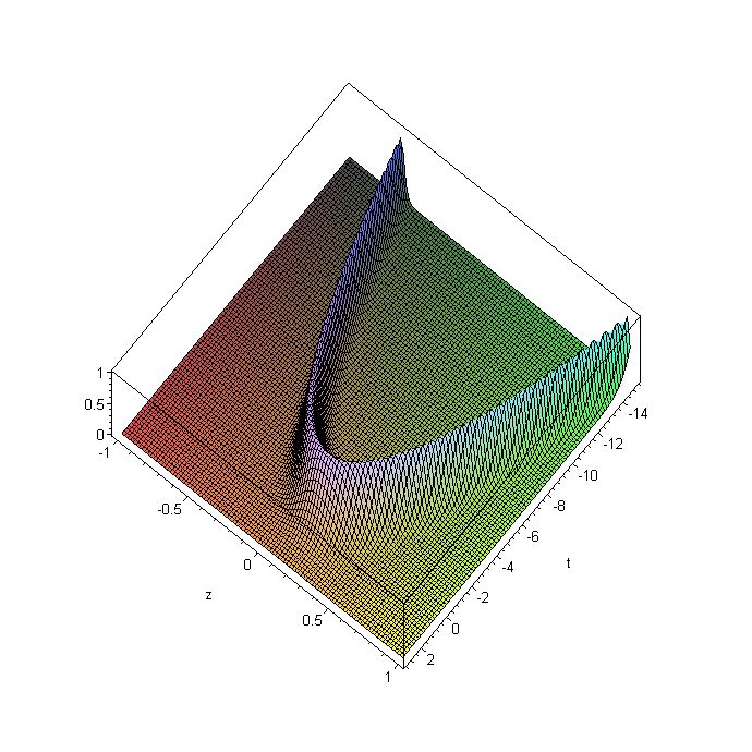
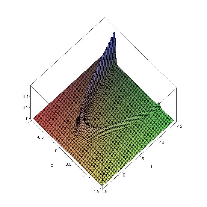
($|E|^{2}$)  ($|p|^{2}$)  ($\eta$)

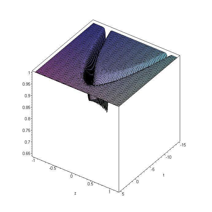
Figure 1. One solition solution $(E,p,\eta)$ of the IH-MB equations when $a_{1}=z,a_{3}=-1,a_{4}=z,a_{7}=z,b_{1}=1,b_{2}=z,\omega=1.5,\alpha_{1}=0.5,\beta_{1}=2,$.

Now let us discuss about the construction of the two-soliton solution of IH-MB system. For the purpose of construction of two soliton solution, we need to use two spectral parameters $\lambda_{1}=\alpha_{1}+\beta_{1}i$ and $\lambda_{2}=\alpha_{2}+\beta_{2}i$. After the second Darboux transformation, we can construct the two solition solution. As the general form of two soliton solution is tedious in nature, for simplicity, we will give only the two soliton solution of E taking values as $a_{1}=z,a_{3}=-1,a_{4}=z,a_{7}=z,b_{1}=1,b_{2}=z,\omega=1.5,\alpha_{1}=0.5,\beta_{1}=2,\alpha_{2}=1,\beta_{2}=1.5$ in appendix.

We also construct two soliton solutions for p and $\eta$ in a similar manner. For completeness, instead of giving complicated forms of p and $\eta$, the graphical representation of them is shown in Fig.2.

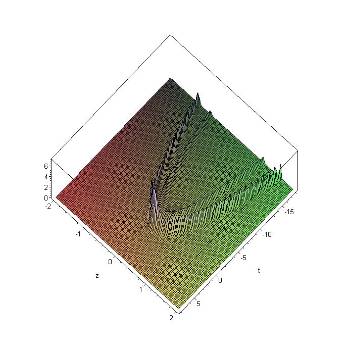
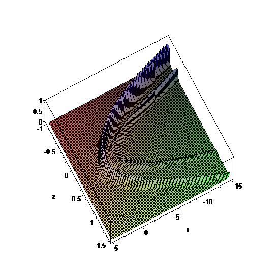
($|E|^{2}$)  ($|p|^{2}$)  ($\eta$)

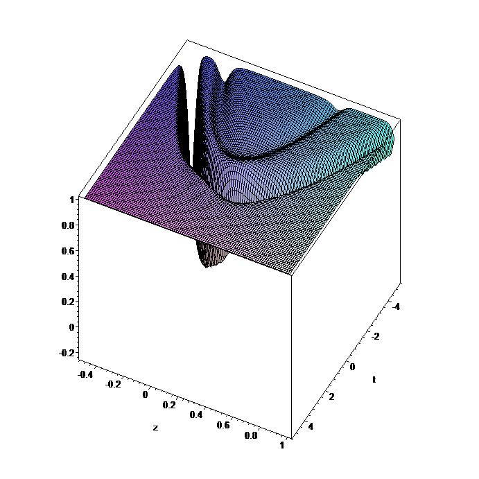
Figure 2. Two solition solution $(E,p,\eta)$ of the IH-MB equations when $a_{1}=z,a_{3}=-1,a_{4}=z,a_{7}=z,b_{1}=1,b_{2}=z,\omega=1.5,\alpha_{1}=0.5,\beta_{1}=2,\alpha_{2}=1,\beta_{2}=1.5$.

If we suppose $a_{1}=0,a_{2}=0,a_{3}=-1,a_{4}=1,a_{5}=6,a_{6}=-2,a_{7}=-2,b_{1}=1,b_{2}=-1,$ this case will go to the classical H-MB equation[31] with constant coefficients.

6. Bright and dark positon solutions of IH-MB system

For the two soliton solution constructed in the last section, if the second spectral parameter $\lambda_{2}$ is close to the first spectral parameter $\lambda_{1}$, doing the Taylor expansion of wave function up to first order near $\lambda_{1}$ will lead to a new kind of solution. This is exactly the so-called positon solutions. In this section, the construction of positon solution of IH-MB equations will be given. Firstly, following four linear functions out of linear system will be used to construct the second Darboux transformation which further generate the positon solutions,

$$\Phi_{1} = \exp(\lambda_{1}t+\int-4\lambda_{1}^{3}a_{4}-2i\lambda_{1}^{2}a_{3}-\lambda_{1}a_{1}-\frac{b_{1}a_{7}}{2\lambda_{1}+2i\omega b_{2}}dz+\frac{x_{0}+iy_{0}}{2}),$$ (6.1)

$$\Phi_{2} = \exp(-\lambda_{1}t+\int 4\lambda_{1}^{3}a_{4}+2i\lambda_{1}^{2}a_{3}+\lambda_{1}a_{1}+\frac{b_{1}a_{7}}{2\lambda_{1}+2i\omega b_{2}}dz-\frac{x_{0}+iy_{0}}{2}+i\theta)$$ (6.2)

$$\Phi_{3} = \exp(\lambda_{2}t+\int-4\lambda_{2}^{3}a_{4}-2i\lambda_{2}^{2}a_{3}-\lambda_{2}a_{1}-\frac{b_{1}a_{7}}{2\lambda_{2}+2i\omega b_{2}}dz+\frac{x_{0}+iy_{0}}{2}),$$ (6.3)

$$\Phi_{4} = \exp(-\lambda_{2}t+\int 4\lambda_{2}^{3}a_{4}+2i\lambda_{2}^{2}a_{3}+\lambda_{2}a_{1}+\frac{b_{1}a_{7}}{2\lambda_{2}+2i\omega b_{2}}dz-\frac{x_{0}+iy_{0}}{2}+i\theta).$$ (6.4)

Then we define the following functions as

$$\Phi_{1,1}:=\phi_{1};\ \Phi_{1,2}:=-\phi_{2}^{*};\ \Phi_{2,1}:=\phi_{2};\ \Phi_{2,2}:=\phi_{1}^{*};$$ (6.5)

$$\Phi_{1,3}:=\phi_{3};\ \Phi_{1,4}:=-\phi_{4}^{*};\ \Phi_{2,3}:=\phi_{4};\ \Phi_{2,4}:=\phi_{3}^{*}.$$ (6.6)

Now we take $\lambda_{2}=\lambda_{1}+\epsilon(1+i)$ and using the Taylor expansion of wave function $\phi_{3}$ and $\phi_{4}$ up to first order of $\epsilon$ in terms of $\lambda_{1}$. Substitution of these manipulations into the second Darboux transformation discussed in the last section will lead to positon solutions. For example, after taking values as $a_{1}=0.5,a_{3}=z,a_{4}=z,a_{7}=1,b_{1}=1,b_{2}=1,\omega=1.5,\alpha_{1}=0.5,\beta_{1}=1,$ i.e. the case of classical H-MB equations[31], the positon solutions $(E_{p},p_{p},\eta_{p})$ can be derived. Here for simplicity, we only give positon solution $E_{p}$ in following form

$$E_{p} = -0.2e^{2it+2.5iz^{2}-0.6153846154iz}[(-130000000000z^{2}+140000000000iz^{2}+11420118340z$$

$$+591715977iz-20000000000t-20000000000)e^{-t-7.500000000z^{2}+0.5769230768z}$$

$$+(591715977iz+140000000000iz^{2}+130000000000z^{2}-11420118340z+20000000000t$$

$$-20000000000)e^{t+7.500000000z^{2}-0.5769230768z}]$$

$$/(2000000000cosh(-15z^{2}+1.153846154z-2t)+4000000000t^{2}+52000000010tz^{2}$$

$$+2000000000-4568047338tz+365000000000z^{4}$$

$$-28035502960z^{3}+1307692307z^{2}).$$

The pictorial representation of positon solutions of the IH-MB equations is shown in Fig.3,

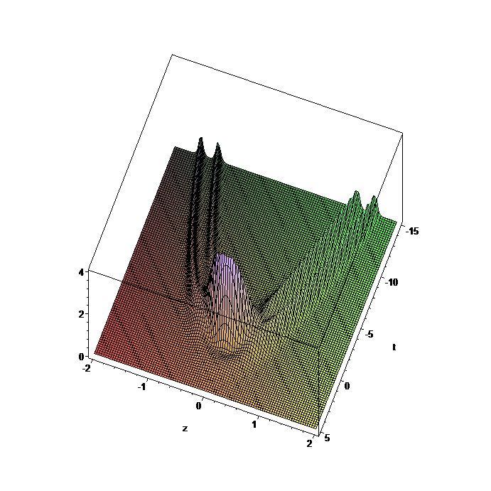
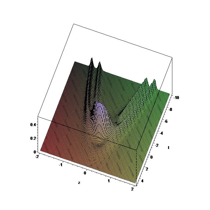
($|E|^{2}$)  ($|p|^{2}$)  ($\eta$)

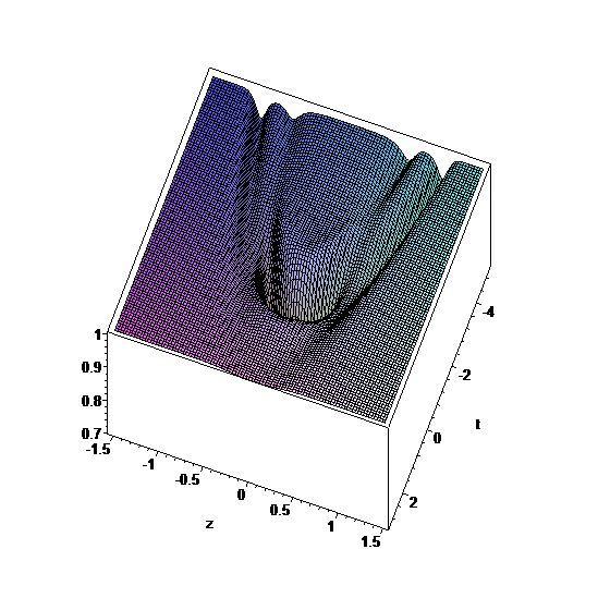
Figure 3. One positon solution $(E,p,\eta)$ of the IH-MB equations when $a_{1}=0.5,a_{3}=z,a_{4}=z,a_{7}=1,b_{1}=1,b_{2}=1,\omega=1.5,\alpha_{1}=0.5,\beta_{1}=1.$

whose density plot is as Fig.4.

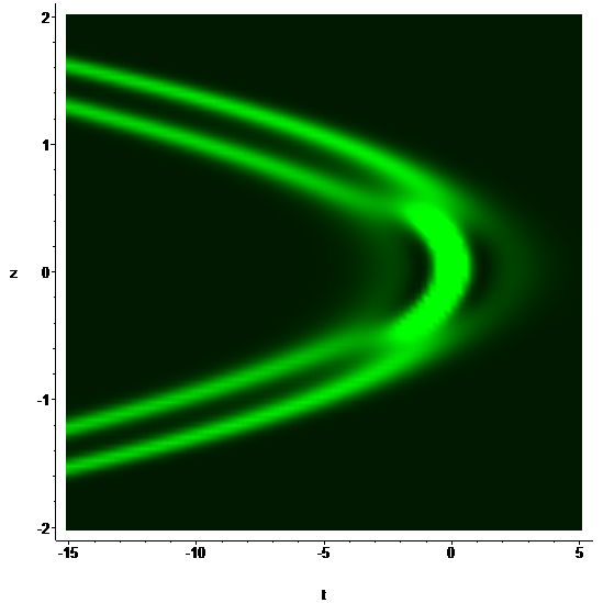
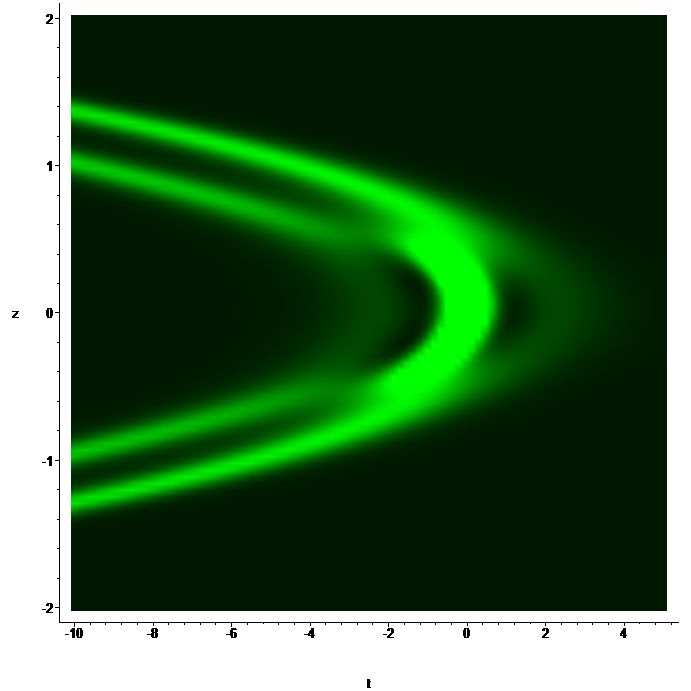
($|E|^{2}$)  ($|p|^{2}$)  ($\eta$)

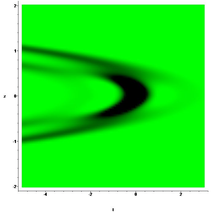
Figure 4. One positon solution $(E,p,\eta)$ of the IH-MB equations when $a_{1}=0.5,a_{3}=z,a_{4}=z,a_{7}=1,b_{1}=1,b_{2}=1,\omega=1.5,\alpha_{1}=0.5,\beta_{1}=1.$

Next, after taking values as $a_{1}=0.5,a_{3}=e^{z},a_{4}=e^{z},a_{7}=1,b_{1}=1,b_{2}=1,\omega=1.5,\alpha_{1}=0.5,\beta_{1}=1$,the picture of positon solutions of the IH-MB equations is as Fig.5,

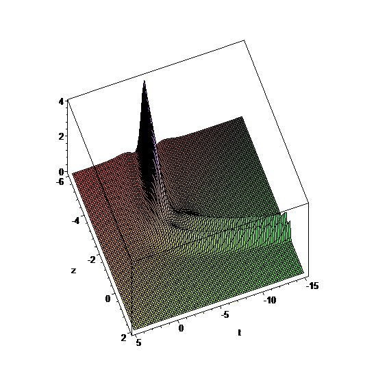
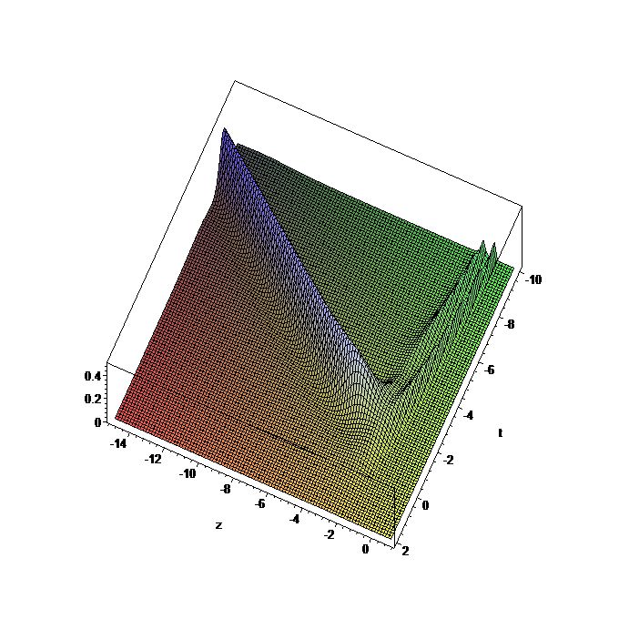
($|E|^{2}$)  ($|p|^{2}$)  ($\eta$) .

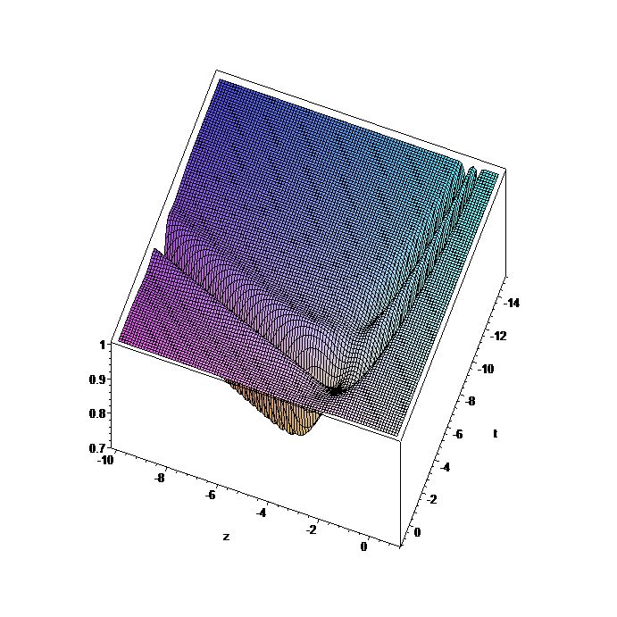
Figure 5. One positon solution $(E,p,\eta)$ of the IH-MB equations when $a_{1}=0.5,a_{3}=e^{z},a_{4}=e^{z},a_{7}=1,b_{1}=1,b_{2}=1,\omega=1.5,\alpha_{1}=0.5,\beta_{1}=1$.

whose density plot is as Fig.6.

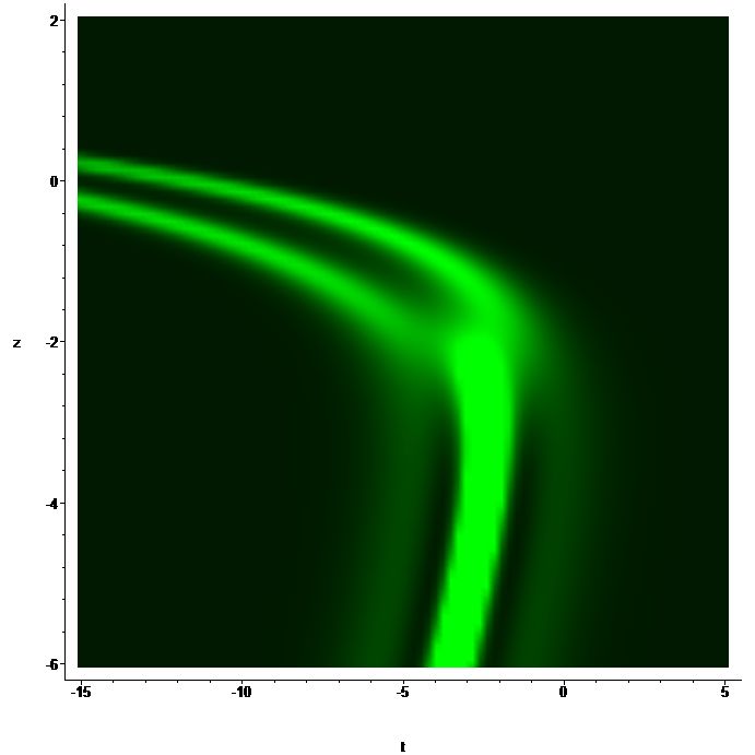
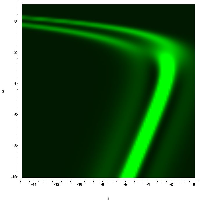
($|E|^{2}$)  ($|p|^{2}$)  ($\eta$) .

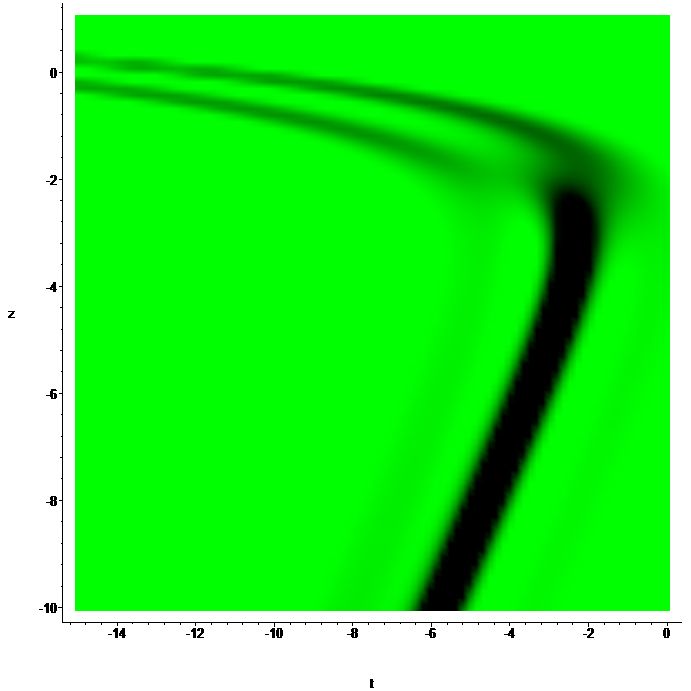
Figure 6. One positon solution $(E,p,\eta)$ of the IH-MB equations when $a_{1}=0.5,a_{3}=e^{z},a_{4}=e^{z},a_{7}=1,b_{1}=1,b_{2}=1,\omega=1.5,\alpha_{1}=0.5,\beta_{1}=1$.

From above we find that $E$ and $p$ are bright positon solutions whereas $\eta$ is a dark positon. In a similar way, using the higher order Darboux transformation, one can also generate higher-order bright and dark positon solutions which will be omitted here. These positons with variable coefficients are different from the classical H-MB equations which can be seen from their graphs.

7. Conclusion and Discussions

In this paper, we derived the Darboux transformation of the inhomogeneous Hirota and the Maxwell-Bloch(IH-MB) equations governed by ultra-short pulse propagation through erbium doped optical waveguide. Further matrix representation of Darboux transformation of this system is constructed. As examples, soliton solutions, positon solutions of the IH-MB equations have been constructed explicitly by using Darboux transformation from trivial solutions seed solutions. There are a few unclear interesting questions such as the physical interpretations and observation of higher-order positon solutions, rogue waves solutions and their applications in physics?

Acknowledgments This work is supported by NSF of Zhejiang Province under Grant No. LY12A01007, the NSF of China under Grant No.11201251, 10971109, K.C.Wong Magna Fund in Ningbo University and Program for NCET under Grant No.NCET-08-0515.

8. Appendix

$$E^{[1]}_{2-sol}$$

$$=[8(17+24z+9z^{2})^{\frac{2}{9}}(13+18z+9z^{2})^{\frac{2}{9}-\frac{1}{3}i}e^{8z-t-\frac{8}{9}arctan(4+3z)-23z^{2}+i(3t-\frac{13}{3}z-6z^{2})}(\frac{1+4i+3iz}{\sqrt{17+24z+9z^{2}}})^{\frac{2}{9}}$$

$$+8(13+18z+9z^{2})^{\frac{2}{9}-\frac{1}{3}i}e^{-8z+t+3it+\frac{8}{9}arctan(4+3z)+23z^{2}-\frac{13}{3}iz-6iz^{2}}(\frac{1+4i+3iz}{\sqrt{17+24z+9z^{2}}})^{\frac{2}{9}}$$

$$-2(13+18z+9z^{2})^{\frac{4}{9}}(17+24z+9z^{2})^{\frac{1}{9}-\frac{4}{9}i}e^{12z-2t+4it-\frac{2}{3}arctan(\frac{3}{2}+\frac{3}{2}z)-22z^{2}-\frac{43}{3}iz+24iz^{2}}(\frac{2+3i+3iz}{\sqrt{13+18z+9z^{2}}})^{\frac{4}{9}}$$

$$-2(17+24z+9z^{2})^{\frac{1}{9}-\frac{4}{9}i}e^{-12z+2t+4it+\frac{2}{3}arctan(\frac{3}{2}+\frac{3}{2}z)+22z^{2}-\frac{43}{3}iz+24iz^{2}}(\frac{2+3i+3iz}{\sqrt{13+18z+9z^{2}}})^{\frac{4}{9}}$$

$$+4i(17+24z+9z^{2})^{\frac{2}{9}}(13+18z+9z^{2})^{\frac{2}{9}-\frac{1}{3}i}e^{8z-t+3it-\frac{8}{9}arctan(4+3z)-23z^{2}-13/3iz-6iz^{2}}(\frac{1+4i+3iz}{\sqrt{17+24z+9z^{2}}})^{\frac{2}{9}}$$

$$+4i(17+24z+9z^{2})^{(}\frac{1}{9}-\frac{4}{9}i)e^{-12z+2t+4it+\frac{2}{3}arctan(\frac{3}{2}+\frac{3}{2}z)+22z^{2}-\frac{43}{3}iz+24iz^{2}}(\frac{2+3i+3iz}{\sqrt{13+18z+9z^{2}}})^{\frac{4}{9}}$$

$$-4i(13+18z+9z^{2})^{(}\frac{2}{9}-\frac{1}{3}i)e^{-8z+t+3it+\frac{8}{9}arctan(4+3z)+23z^{2}-13/3iz-6iz^{2}}(\frac{1+4i+3iz}{\sqrt{17+24z+9z^{2}}})^{\frac{2}{9}}$$

$$-4i(13+18z+9z^{2})^{\frac{4}{9}}(17+24z+9z^{2})^{\frac{1}{9}-\frac{4}{9}i}e^{12z-2t+4it-\frac{2}{3}arctan(\frac{3}{2}+\frac{3}{2}z)-22z^{2}-\frac{43}{3}iz+24iz^{2}}(\frac{2+3i+3iz}{\sqrt{13+18z+9z^{2}}})^{\frac{4}{9}}]$$

$$/[(\frac{2+3i+3iz}{\sqrt{13+18z+9z^{2}}})^{\frac{4}{9}}(\frac{1+4i+3iz}{\sqrt{17+24z+9z^{2}}})^{\frac{2}{9}}(-8(13+18z+9z^{2})^{\frac{2}{9}}(17+24z+9z^{2})^{\frac{1}{9}}cos$$

$$(t+\frac{4}{9}arctan(\frac{3}{2}+\frac{3}{2}z)+\frac{1}{3}ln(13+18z+9z^{2})-10z+30z^{2}-\frac{2}{9}arctan(4+3z)-\frac{4}{9}ln(17+24z+9z^{2}))$$

$$+5(17+24z+9z^{2})^{\frac{2}{9}}e^{-4z+t+\frac{2}{3}arctan(\frac{3}{2}+\frac{3}{2}z)-\frac{8}{9}arctan(4+3z)-z^{2}}+e^{-20z+3t+\frac{2}{3}arctan(\frac{3}{2}+\frac{3}{2}z)+\frac{8}{9}arctan(4+3z)+45z^{2}}$$

$$+5(13+18z+9z^{2})^{\frac{4}{9}}e^{4z-t-\frac{2}{3}arctan(\frac{3}{2}+\frac{3}{2}z)+\frac{8}{9}arctan(4+3z)+z^{2}}$$

$$+(13+18z+9z^{2})^{\frac{4}{9}}(17+24z+9z^{2})^{\frac{2}{9}}e^{20z-3t-\frac{2}{3}arctan(\frac{3}{2}+\frac{3}{2}z)-\frac{8}{9}arctan(4+3z)-45z^{2}})].$$

References

- [1] P. Müller, C. Garrett and A. Osborne, Oceanography, 18(2005), 66.
- [2] A. Osborne, Nonlinear Ocean Waves and the Inverse Scattering Transform (Elsevier, New York, 2010).
- [3] L. Wen, L. Li, Z. D. Li, S. W. Song, X. F. Zhang, W. M. Liu, Matter rogue wave in Bose-Einstein condensates with attractive atomic interaction, Eur. Phys. J. D, 64(2011), 473.
- [4] L. Li, B. A. Malomed, D. Mihalache, W. M. Liu, Exact soliton-on-plane-wave solutions for two-component Bose-Einstein condensates, Phys. Rev. E, 73(2006), 066610.
- [5] Z. X. Liang, Z. D. Zhang, W. M. Liu, Dynamics of a bright soliton in Bose-Einstein condensates with time-dependent atomic scattering length in an expulsive parabolic potential, Phys. Rev. Lett. 94(2005), 050402.
- [6] L. Li, Z. D. Li, B. A. Malomed, D. Mihalache, W. M. Liu, Exact soliton solutions and nonlinear modulation instability in spinor Bose-Einstein condensates, Phys. Rev. A, 72(2005), 033611.
- [7] S. W. Xu, J. S. He and L. H. Wang, The Darboux transformation of the derivative nonlinear Schrödinger equation, J. Phys. A: Math. Theor. 44 (2011),305203.
- [8] S. W. Xu, J. S. He, The rogue wave and breather solution of the Gerdjikov-Ivanov equation,J. Math. Phys.53(2012), 063507.
- [9] J. S. He, H. R. Zhang, L. H. Wang, K. Porsezian, A. S. Fokas, A generating mechanism for higher order rogue waves, arXiv:1209.3742.
- [10] A. Hasegawa and F. Tappert, Transmission of stationary nonlinear optical pulses in dispersive dielectric fibers.I.Anomalous dispersion, Appl.Phys.Lett. 23(1973), 142-144.
- [11] M. McCall and E. L. Hahn, Self-induced transparency by pulsed coherent light, Phys. Rev. Lett., 18(1967), 908.
- [12] S. P. Burtsev and I. R. Gabitov, Alternative integrable equations of nonlinear optics, Phys. Rev. A, 49(1994), 2065.
- [13] M. Nakazawa, Y. Kimura, K. Kurokawa and K. Suzuki, Self-induced-transparency solitons in an erbium-doped fiber waveguide, Phys. Rev. A, 45(1992), R23.
- [14] M. Nakazawa, K. Suzuki, Y. Kimura and H. Kubota, Coherent -pulse propagation with pulse breakup in an erbium-doped fiber waveguide amplifier, Phys. Rev. A, 45(1992), R2682
- [15] C. G. L. Tiofack, T. B. Ekogo, A. Mohamadou, K. Porsezian, and Timoleon C. Kofane, Dynamics of bright solitons and their collisions for the inhomogeneous coupled nonlinear Schrödinger-Maxwell-Bloch equations, submitted.
- [16] J. S. He, Y. Cheng and Y. S. Li, The Darboux Transformation for NLS-MB Equation. Commun. Theor. Phys. (2002),493-496.
- [17] J. S. He, S. W. Xu,and K. Porsezian, New Types of Rogue Wave in an Erbium-doped fibre system, J. Phs. Soc. Japan, 81(2012), 033002.
- [18] R. Vasantha Jayakantha Raja, K. Porsezian, Shailendra K. Varshney, S. Sivabalan,Modeling photonic crystal fiber for efficient soliton pulse propagation at 850 nm, Optics Communications 283 (2010) 5000-5006.
- [19] Amitava Choudhuri, K. Porsezian, Dark-in-the-Bright solitary wave solution of higher-order nonlinear Schrödinger equation with non-Kerr terms Optics Communications 285 (2012) 364-367.
- [20] P. Tchofo Dinda1, K. Porsezian, Impact of fourth-order dispersion in the modulational instability spectra of wave propagation in glass fibers with saturable nonlinearity, J. Opt. Soc. Am. B, 27(2010).
- [21] K. Nakkeeran and K. Porsezian, Solitons in an erbium-doped nonlinear fibre medium with stimulated inelastic scattering, J. Phys. A: Math. Gen. 28(1995),3817.
- [22] K. Porsezian and K. Nakkeeran, Optical solitons in erbium-doped nonlinear fibre medium with higher order dispersion and self-steepening, 1995 J. Mod. Opt. 43, 693-699.
- [23] K. Nakkeeran, Optical solitons in erbium-doped fibres with higher-order effects and pumping, J. Phys. A: Math. Gen., 33(2000), 4377-4381.
- [24] Y. Kodama, Normal forms for weakly dispersive wave equations, Phys. Lett. A 112(1985), 193-196.
- [25] R. Hirota, Exact envelopesoliton solutions of a nonlinear wave equation, J. Math. Phys. 14(1973), 805.
- [26] A. Ankiewicz, J. M. Soto-Crespo, and N. Akhmediev, Rogue waves and rational solutions of the Hirota equation, Phys. Rev. E 81, 046602(2010).
- [27] Y. S. Tao, J. S. He, Multisolitons, breathers, and rogue waves for the Hirota equation generated by the Darboux transformation, 85, 026601 (2012).
- [28] K. Porsezian and K. Nakkeeran, Optical Soliton Propagation in an Erbium Doped Nonlinear Light Guide with Higher Order Dispersion, Phys. Rev. Lett. 74(1995), 2941.
- [29] V. B. Matveev, M. A. Salle, Darboux transformations and solitons,Springer, Berlin(1991).
- [30] J. S. He, L. Zhang, Y. Cheng and Y. S. Li, Determinant representation of Darboux transformation for the AKNS system, Sci. China A, 12(2006), 1867-78.
- [31] C. Z. Li, J. S. He and K. Porsezian, Rogue waves of the Hirota and the Maxwell-Bloch equation, arXiv:1205.1191.
- [32] Z. Y. Yan, Nonautonomous “rogons” in the inhomogeneous nonlinear Schrödinger equation with variable coefficients, Phys. Lett.A. 374(2009), 672-679.
- [33] C. G. Latchio Tiofack, T. B. Ekogo, Alidou Mohamadou, K. Porsezian, and Timoleon C. Kofane, Dynamics of bright solitons and their collisions for the inhomogeneous coupled nonlinear Schrödinger-Maxwell-Bloch equations, in preparation.
- [34] Y. S. Xue, B. Tian, etal., Soliton interactions in a generalized inhomogeneous coupled Hirota-Maxwell-Bloch system, Nonlinear Dynamics, 67(2011), 2799-2806.
- [35] J. R. Taylor, Optical Solitons: Theory and Experiment. Cambridge University, Cambridge(1992).
- [36] F. M. Mitschke, L. F. Mollenauer: Discovery of the soliton self-frequency shift. Opt. Lett. 11(1986), 657-659.
- [37] B. L. Guo, L. M. Ling and Q. P. Liu, Nonlinear Schrödinger Equation: Generalized Darboux Transformation and Rogue Wave Solutions, Phys. Rev. E, 85(2012), 026607.
- [38] C. Q. Dai, J. F. Zhang, New solitons for the Hirota equation and generalized higher-order nonlinear Schröinger equation with variable coefficients. J. Phys. A 39(2006), 723-737.