The challenge of large and empty voids in the SDSS DR7 redshift survey

Abstract

Context. We present catalogues of voids for the SDSS DR7 redshift survey and for Millennium I simulation mock data.

Aims. We aim to compare the observations with simulations based on a $\Lambda$CDM model and a semi-analytic galaxy formation model. We use the void statistics as a test for these models.

Methods. We assembled a mock catalogue that closely resembles the SDSS DR7 catalogue and carried out a parallel statistical analysis of the observed and simulated catalogue.

Results. We find that in the observation and the simulation, voids tend to be equally spherical. The total volume occupied by the voids and their total number are slightly larger in the simulation than in the observation. We find that large voids are less abundant in the simulation and the total luminosity of the galaxies contained in a void with a given radius is higher on average than observed by SDSS DR7 survey. We expect these discrepancies to be even more significant in reality than found here since the present value of $\sigma_{8}$ given by WMAP7 is lower than the value of $0.9$ used in the Millennium I simulation.

Conclusions. The reason why the simulation fails to produce enough large and dark voids might be the failure of certain semi-analytic galaxy formation models to reduce the small-scale power of $\Lambda$CDM and to produce sufficient power on large scales.

1 Introduction

Redshift surveys have been demonstrating for several decades that galaxies are distributed on a cosmic web of filaments, walls, and clumps. These structures, which form on a hierarchy of scales and span a wide redshift range, border low-luminosity regions that are mostly devoid of observable galaxies. These “void” regions occupy more than $80\%$ of the volume of the observable Universe. Since the discovery of voids using Zwicky clusters (Einasto et.al., 1980) and the discovery of the first giant or supervoid in the Bootes constellation (Kirshner et al., 1981) numerous works have followed (Zeldovich et al., 1982; Davis et al., 1982; de Lapparent et al., 1986; da Costa et al., 1988; Geller & Huchra, 1989; da Costa et al., 1994) and diverse algorithms for void identification have been developed and applied to larger and more complete surveys (see Colberg et al. (2008) for a summary and comparison of different methods).

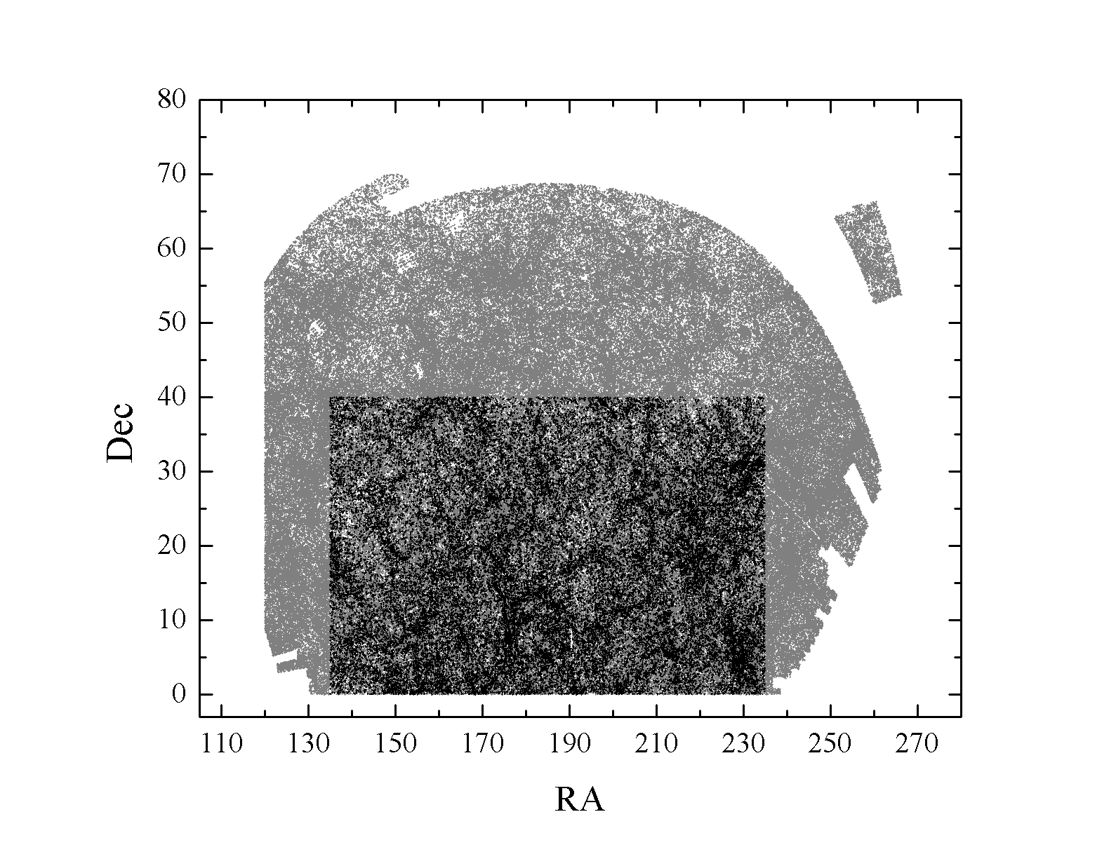
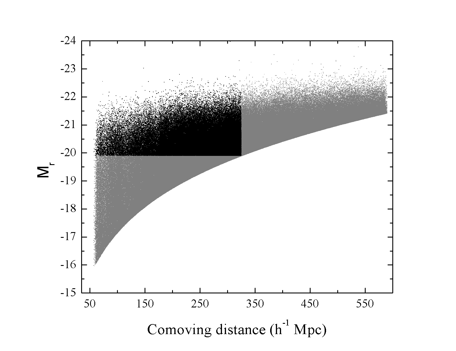
Figure 1: Darker shaded areas in the two panels show the SDSS DR7 region (left) and the volume-limited sample (right) that we selected for this work.

The formation and evolution of voids is well-understood in the framework of gravitational instability (Zeldovich et al., 1982; Shandarin & Zeldovich, 1989). However, when one compares void properties of observations and simulations based on $\Lambda$CDM, certain problems still remain to be better understood. By definition, voids are devoid of galaxies or contain only a negligible number of faint galaxies. The perplexing issue is that we do not see a large population of low-mass galaxies populating voids (Klypin et.al. (1999); Moore et.al. (1999)), and furthermore, the void galaxies that we do see are basically representative of the general population (Peebles, 2001).

Observed voids seem to contain fewer galaxies and in particular dwarf galaxies, contrary to what is expected from $\Lambda$CDM (Peebles, 2001; Tully et al., 2008; Tikhonov & Klypin, 2009). Some studies have also shown that voids in observations are significantly larger than those in simulations (Ryden & Turner, 1984). Although modifying models of galaxy formation might solve these problems and various remedies such as proper biasing and halo occupation distribution have been proposed (Hoyle et al., 2005; Tinker et al., 2008), different studies suggest that the problem would still persist (Bothun et al., 1986; Little & Weinberg, 1994; Plionis & Basilakos, 2002; Gottlöber et al., 2003; Hoyle & Vogeley, 2004; Goldberg et al., 2005; Hoeft et al., 2006).

The problem of empty and large voids could arise because the $\Lambda$CDM has too much power on small scales which would in turn lead to the problem of over-abundance of substructures (Tikhonov & Klypin, 2009). Substructures would occupy the voids, making them less empty, and statistically, they could break larger voids into smaller ones. On the other hand, one could equally infer that $\Lambda$CDM lacks power on large scales, perhaps because the value of $\sigma_{8}$ is too low.

In this work, we study this problem by analysing voids in the SDSS DR7 data and by carrying out a parallel and comparative analysis on a mock-SDSS DR7 catalogue based on the Millennium I simulation. Our void-finder algorithm is an improved and generalised version of the original algorithm proposed by Aikio & Maehoenen (1998). The important feature of this algorithm is that it does not assume a priori that voids are spherical and hence can be used to study the shapes of the voids. We apply our void-finder algorithm to the Sloan Digital Sky Survey SDSS DR7 and build a catalogue of voids. In parallel, we also apply our algorithm to a mock-SDSS DR7 catalogue, which we construct out of the Millennium I simulation. The mock catalogue is given the same magnitude cut-off as SDSS DR7. In a different version, we also set up a mock catalogue with the same number density as SDSS, but a different magnitude cut-off. This allows us to compare various properties of observed voids to those predicted by $\Lambda$CDM and the semi-analytic model of galaxy formation.

In Section 2, we present our sample taken from the SDSS DR7 catalogue. In Section 3, we present our mock catalogue. In Section 4, we explain our void-finder algorithm. In Section 5, we find the voids in the simulation and observation catalogues and discuss the numbers, sizes, and shapes of the voids. In Section 6, we study the abundance of large voids in the observations and the mock catalogues. In Section 7, luminosities of voids as a function of their sizes are presented and compared between the simulation and the observation. In Section 8, we conclude.

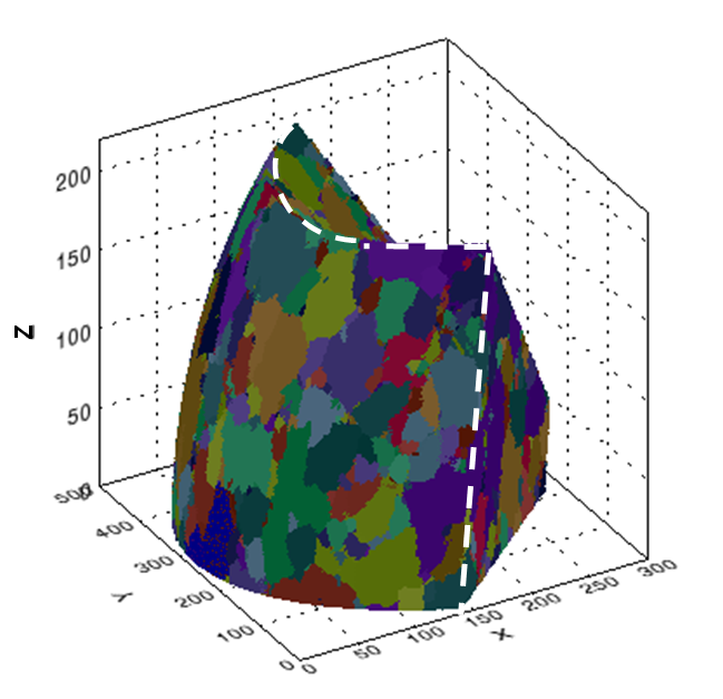
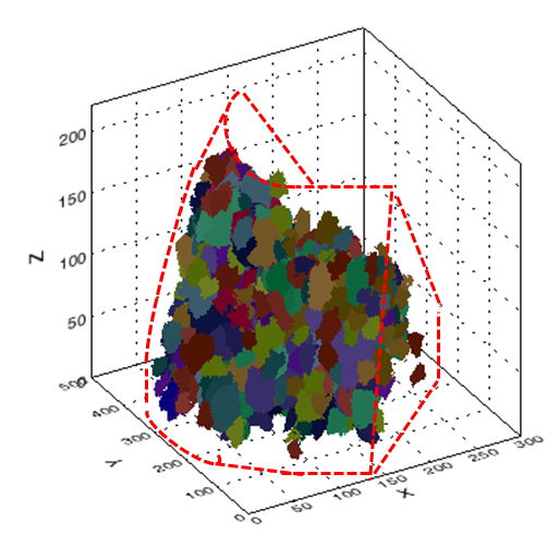
Figure 2: Right panel: initial voids in the observational data of SDSS DR7. Left panel: final voids after without small and edge voids.

2 SDSS DR7: definition of the sample

We have selected the main galaxy sample of the seventh data release of the Sloan Digital Sky Survey (SDSS DR7) (Abazajian et al., 2009). The galaxy redshifts were corrected for the motion of the local group and are given in the CMB rest frame. The k-corrections for the SDSS galaxies were calculated using the KCORRECT algorithm developed by Blanton et.al. (2003a) and Blanton & Roweis (2007). The boundaries of our selected region of SDSS are: $135<{\rm RA}<235$ and $0<{\rm DEC}<40$, which contains 283076 galaxies. The choice of boundaries clearly is arbitrary. However, the selected region in our study covers most of SDSS DR7. We used spectroscopic data and applied a void algorithm to volume-limited samples. Had we selected high-redshift galaxies, we would have had to consider very bright galaxies (M ¡ -21, -22), which would be meaningless for voids. All objects in this selected region have a redshift error smaller than $2.5\times 10^{-4}$ and the errors in their apparent ”Petrosian” magnitudes of the r band, $m_{r}$, are smaller than $0.1$. The absolute magnitudes of the galaxies were determined in the r band using cosmological parameters; $H_{0}=100$ and the density parameters $\Omega_{m}=0.25$ and $\Omega_{\Lambda}=0.75$. Galaxies belonging to voids were identified by using a volume-limited sample taken from the selected region. The final subsample contains 68702 galaxies with absolute magnitudes $M_{r}<-19.9$, which lie in the comoving distance interval 75-325 h^-1Mpc, corresponding to $0.02<z<0.12$.

The selected region of the SDSS DR7 is shown in the left panel of Fig. 1. The right panel of this figure shows the plot of the absolute r-band magnitude versus comoving distance. The dark region in this plot illustrates the selected volume-limited sample we used.

3 Mock Millennium I catalogue: definition of the sample

The Millennium I simulation was with a $N=2160^{3}$ particles in a comoving box of length $L=500h^{-1}{\rm Mpc}$ and mass resolution of $8.6\times 10^{8}h^{-1}M_{\odot}$. The adopted cosmology is a $\Lambda$CDM model with $\Omega_{m}=0.25$, $\Omega_{b}=0.045,\Omega_{\Lambda}=0.75,h=0.73,n=1$ and $\sigma_{8}=0.9$. This value of $\sigma_{8}$ is higher than its present value of $0.8$ given by WMAP7 (Komatsu et.al., 2011), hence yielding more power on larger scales. The evolution of baryons within these dark matter halos is predicted by different semi-analytic models. Current semi-analytic models try to incorporate various complex processes such as gas cooling, reionization, star formation, supernova feedback, metal evolution, black hole growth, and active galactic nuclei (AGN) feedback (e.g. Bower et.al. (2006),De Lucia & Blaizot (2007),Guo et al. (2011)). Although the semi-analytic models are designed to match the observational data as closely as possible, they can still fail in certain aspects, for example the low-mass galaxies with stellar-mass ($<10^{9}M_{\odot}$) are slightly over-predicted. Consequently, to remedy this problem, supernova feedback, a modified law for star formation, or a different cosmological model are evoked (see e.g. Guo et al. (2011); Bower et al. (2012); Wang et al. (2012); Menci et.al. (2012)).

In this work, we used the mock galaxy redshift catalogue of the Blaizot-ALLSky-PT-1 ¹ , which was designed to mimic the SDSS and has an almost identical redshift distribution and a very similar colour distribution. This mock catalogue was constructed by Blaizot et al. (2005) using the mock map facility (MoMaF) code and the semi-analytic model presented in De Lucia & Blaizot (2007). Furthermore, to have a mock catalogue that resembles the SDSS DR7 galaxy survey as closely as possible, we selected a region in the simulation that lies in the same redshift range ($0.02<z<0.12$) and has the same geometry. Our mock volume-limited sample includes 68701 galaxies with stellar masses larger than $10^{9}M_{\odot}$ and brighter than $M_{r}<-20.16$, roughly representing the galaxies brighter than $M_{r}<-19.9$ in the SDSS DR7 sample and covering a volume of $1.2\times 10^{7}{\rm(Mpc/h)^{3}}$ in the volume-limited SDSS DR7. Consequently, the simulation sample has the same galaxy number density as the SDSS DR7 sample.

Table 1: Characteristics of our volume-limited samples.

	${\,{\rm Observation}}$	${\,{\rm Simulation}}$
${\rm Sample\,\,Volume\,\,}({\rm Mpc/h})^{3}$	$\approx 1.2\times 10^{7}$	$\approx 1.2\times 10^{7}$
${\rm Number\,\,of\,\,galaxies}$	68702	68701
${\rm Number\,\,of\,\,field\,\,galaxies}$	5873	5377
${\rm Number\,\,of\,\,wall\,\,galaxies}$	62829	63324
${\rm Number\,\,of\,\,void\,\,galaxies(field+faint)}$	26859	43666
${\rm Mean\,\,galaxy\,\,separation\,\,}({\rm Mpc/h})$	6.22	6.35

4 Void-finder algorithm

Various definitions of voids have been suggested previously (Kirshner et al., 1981; Kauffmann & Fairall, 1991; Sahni et al., 1994; Benson et al., 2003) and a number of void-finding algorithms, some which assuming voids to be nearly spherical, have been developed (see e.g. Hoyle & Vogeley (2002)). We developed a method that does not assume a priori that voids are spherical, and is based on the original algorithm of Aikio & Maehoenen (1998). (Hereafter AM algorithm). The AM algorithm was originally written in 2D. We extended it to 3D and adapted it for application to large datasets. The algorithm does not constrain the voids to be of any particular shape and hence can be used to study the shapes of the voids and their deviations from sphericity. We emphasise that here we consider the Aikio-Maehoenen statistics only as a tool for the relative measurement of some parameters of voids (eg. sphericity) in observational and simulated catalogues, and not as tool which would provide any absolute measurements.

Prior to applying of AM algorithm to our volume-limited galaxy sample, we classified galaxies as wall or field galaxies. To distinguish between wall and field galaxies, we introduced the parameter $d$, which is related to the mean distance of the third-nearest neighbour, $d_{3}$, and the standard deviation of its value, $\sigma$, by the following expression: ($d=d_{3}+1.5\sigma$) (Hoyle & Vogeley, 2002). In our volume-limited galaxy sample, all galaxies with a third-nearest neighbour distance, $d_{3}$, greater than this selection parameter, $d$, were taken to be field galaxies and removed from the galaxy sample. The remaining objects were identified as wall galaxies. We remark that a field galaxy may lie within a void region, hence a void galaxy, whereas wall galaxies all lie in the cosmic filaments and clusters and by definition are not to be found in voids.

We found that the selection parameters, $d$, for observation and simulation data are 5.96 and 6.16 Mpc/h, respectively, which means that $9\%$ of the galaxies in the observation and $8\%$ in the simulation are identified as field galaxies. The details of the samples are given in Table 1.

To implement the AM algorithm, the wall galaxies were gridded up in cells of size 1 Mpc/h. The AM algorithm starts on the Cartesian gridded wall galaxy sample by defining a distance field (DF). For a given grid in a 3D galaxy sample the DF was defined as the distance to the nearest particle. Then according to the value of DF for the closest neighbours of each grid, the local maximum of the DF subvoid was calculated. To assign each element in the grid sample to a subvoid, we employed the climbing algorithm (Schmidt et al., 2001) where for a unit cell bounded by the grid points, i.e. an elementary cell, the gradient in DF to each of the neighbouring cell is calculated. In this method, the elementary cell and every other cell along the climbing route is then assigned to a subvoid. Finally, if the distance between two subvoids is less than both DFs, they will be joined into a larger void.

Table 2: Statistics of voids in the observation of SDSS DR7 and the mock simulation catalogue

		Observation			Simulation
		Number	Volume (Mpc/h)3		Number	Volume (Mpc/h)3
All voids		4616	12541454		4847	12555147
Edge voids		1148	7844214 $(62.5\%)$		1193	7646672 $(61\%)$
Small voids $(r_{eff}<7{\rm Mpc/h})$		3001	722062 $(5.8\%)$		3085	845753 $(6.7\%)$
Voids in the final sample		467	3975178 $(31.7\%)$		569	4062722 $(32.3\%)$

The void volume was estimated using the number of grid points inside a given void multiplied by the volume associated with the grid cell. For each void, we defined its effective radius ($r_{\rm eff}$) as the radius of a sphere whose volume is equal to that of the void.

The configuration of each void in this algorithm depends on the grid points, and subsequently we determined the void centre as the centre of mass identified by the positions of the grid points that enclose an elementary cell. Following this standard method and giving the same weight to all elementary cells, the centre of each void can be written as

$$\ X_{V}^{j}=1/N\sum_{i=1}^{N}x_{i}^{j},\$$ (1)

where $x_{i}^{j}$ $(j=1,2,3)$ are the locations of elementary cells and $\it N$ is the number of cells in the void $\it V$. The shape of a voids is then characterised by the ratio of the total number of grid points, which lie between its centre and its effective radius, to its volume. This ratio is an indicator of the deviation of the void shape from sphericity. Ideally, for a spherical void this ratio is equal to one.

In the next section, we apply this algorithm to the SDSS DR7 and the mock catalogue to construct catalogues of voids and study their characteristics.

5 Voids in the SDSS DR7 redshift survey and in the mock catalogue

Table 3: Sizes and sphericities of voids in the observation and simulation mock catalogues

		Effective radius $({\rm Mpc/h})$				Max-length $({\rm Mpc/h})$				Surface $({\rm Mpc/h})^{2}$				Sphericity
		Max	Min	Median		Max	Min	Median		Max	Min	Median		Max	Min	Median
Observation		30.47	7.02	9.65		108.6	19.9	32.3		35414	1214	2588		0.82	0.22	0.71
Simulaion		28.15	7.00	9.08		103.1	19.1	30.1		33018	1210	2276		0.84	0.12	0.72

We identified 4616 and 4847 voids of different sizes and shapes in the SDSS DR7 survey and in the mock catalogue, respectively. We avoided problems due to boundary effects by selecting voids that lie completely inside the geometrical boundaries of our catalogues. Therefore, edge voids, those that touch the survey boundaries, are removed from our void catalogue because of their under-estimated volumes and distorted shapes (see Fig.2).

The size of each void is characterised by its effective radius, defined in the previous section. To avoid counting spurious voids, we set a threshold of 7 Mpc/h for the minimum size of effective radii of voids in both samples. This threshold is higher than mean distance between galaxies in the sample and helps to eliminate seemingly small voids from the sample. After removing all spurious voids, we had about 467 and 569 voids in our volume-limited sample of the SDSS DR7 survey and the mock simulation data, respectively, which occupy $\sim 32\%$ of the volumes of the samples. In Table 2, we provide the void statistics. Hereafter all analyses are carried out on voids in the final sample, obtained after eliminating small and edge voids.

Table 3 compares the statistical properties of voids in the observed and mock catalogues. It shows that the median of void sphericity in both samples is nearly $\sim 0.70$, which indicates that voids tend to be mostly spherical. Fig. 3 also shows that voids tend to become more spherical with increasing radii. There is a good agreement between the mock catalogue and the SDSS observation, although the observed voids seem to be marginally more spherical in general. More and better data are needed to see if the marginal difference reported here is of any significance.

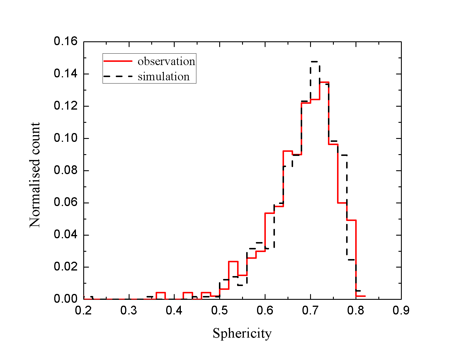
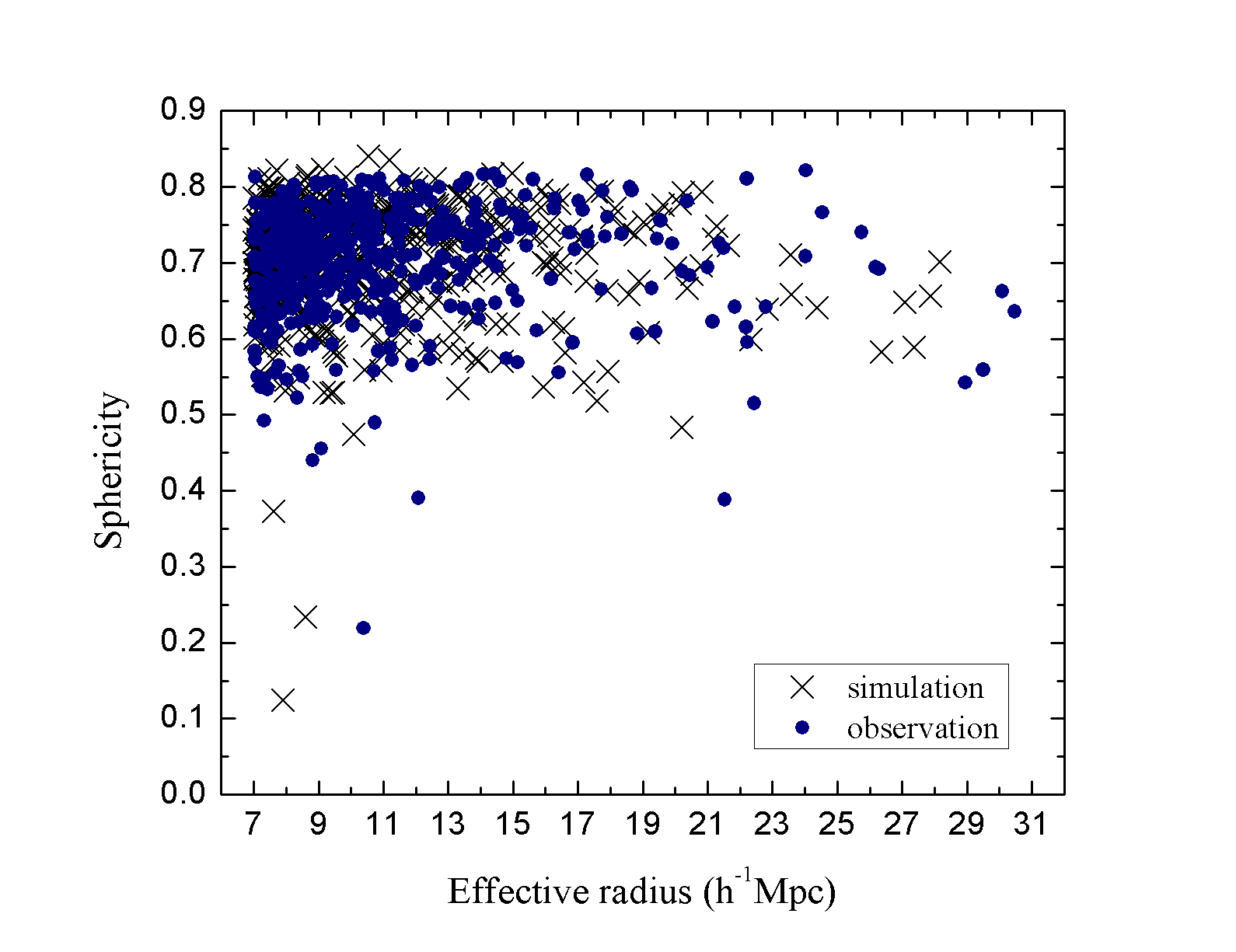
Figure 3: Left panel: distribution of sphericity is skewed towards larger sphericities, i.e. voids are mostly spherical. Right panel: plot of the sphericities versus the equivalent radii of the voids, demonstrating that voids become more spherical with increasing radii. There is no significant difference between the observation and the simulation and more data would be needed to establish any disagreement between the two.

6 Abundance of large voids: the SDSS DR7 observation versus the mock catalogue

We compared the distribution of the void sizes in the observation with the simulated mock catalogues. Fig. 4 shows that the volume occupied by voids is larger in the simulation than in the observation. In particular, both the histograms and the commulative plots show that the largest voids are absent from the simulation, whereas they are present in the observation.

The problem of large voids could be related to the over-abundance of small galaxies, which would subsequently divide large voids into smaller ones. However, this could be resolved by proper biasing in modelling the galaxy formation and evolution. Hence, the problem of large voids could be due to the shortcoming of the semi-analytic model of galaxy formation for the mock catalogue that we used here. A recent study that also compared the SDSS DR7 voids with those taken from a smoothed particle hydrodynamics (SPH) simulation and a halo-occupation model and hence used a different model of galaxy evolution, seems to indicate that the distribution of the void sizes agree in the two samples (Pan et al., 2012). Hence, these void properties could be of potential importance in distinguishing between different galaxy formation scenarios.

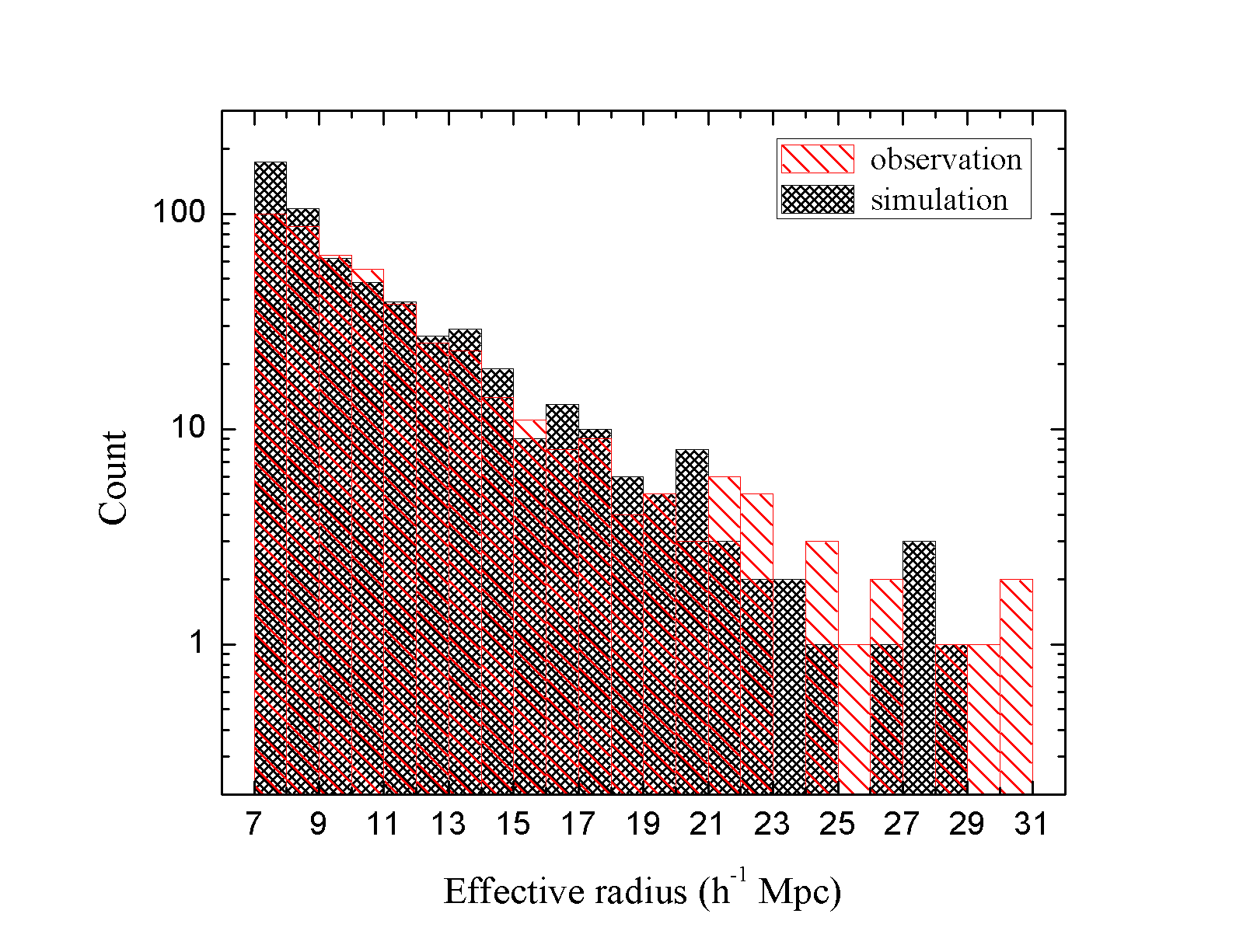
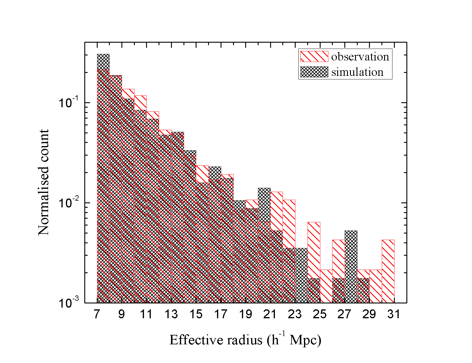
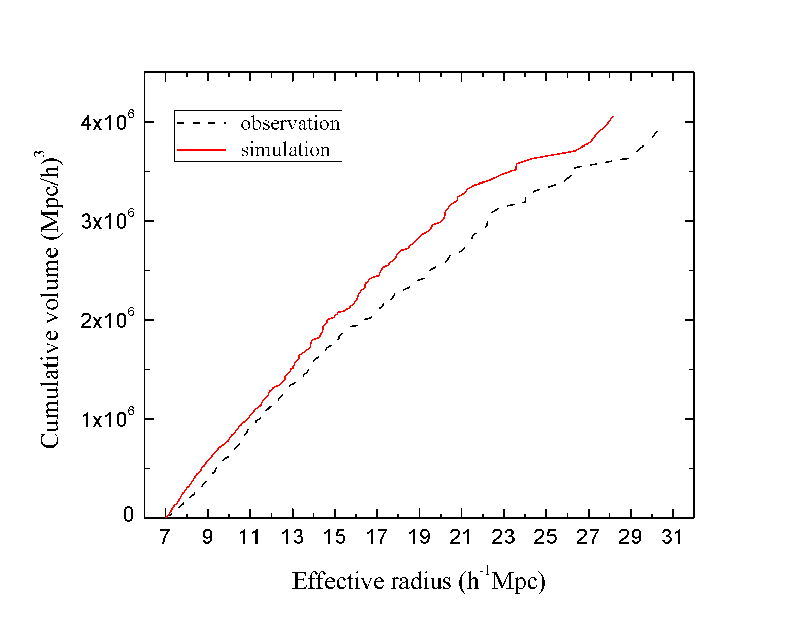
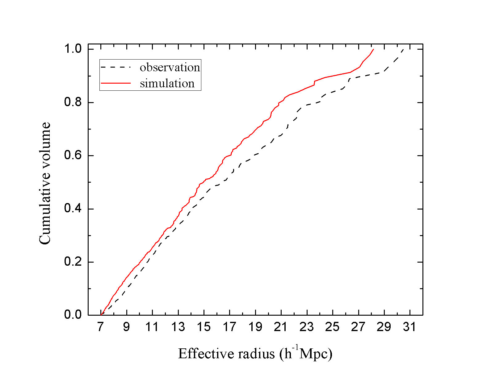
Figure 4: Top panel: Distribution of the void sizes in the observation and the simulation: larger voids are more abundant in the observation. Bottom panel: Cumulative plots of the number of voids against their equivalent radii shows again that larger voids are more abundant in the observation. The bottom plots show the volume/radius cumulative curves where both the commulative volume and normalised volumes are plotted against the effective radii of the voids. The histograms show that at large radii, there are more voids in the observation than in the simulation. The lower panels demonstrate that the number and volume of voids are, in general, higher in the simulation than in the observation (see Table.2). Because there are only two catalogues, we cannot perform a proper error analysis and determine the error bars in these figures. However, we performed a Kolmogorov-Smirnov test that shows that the probability of the two samples to have similar distributions is only about 0.004 and hence the difference between the two catalogues reported in these figures is statistically significant.

7 Observed SDSS voids are less luminous than those in the mock catalogue

Prior to comparing the luminosities of the voids between simulation and observation, we checked that there was no bias between the two samples. In Fig. 5, we plotted the histogram of the absolute magnitudes of field and faint galaxies that are found in the voids in the two catalogues. The figure shows that although there are more void galaxies in the mock catalogue than in the observation, the distributions are the same in both catalogues. Min and max magnitudes are nearly the same, namely $M\sim-16.5$ in the and M$\sim$ -22 in the observation and the simulation. This demonstrates that there is no bias between the two samples.

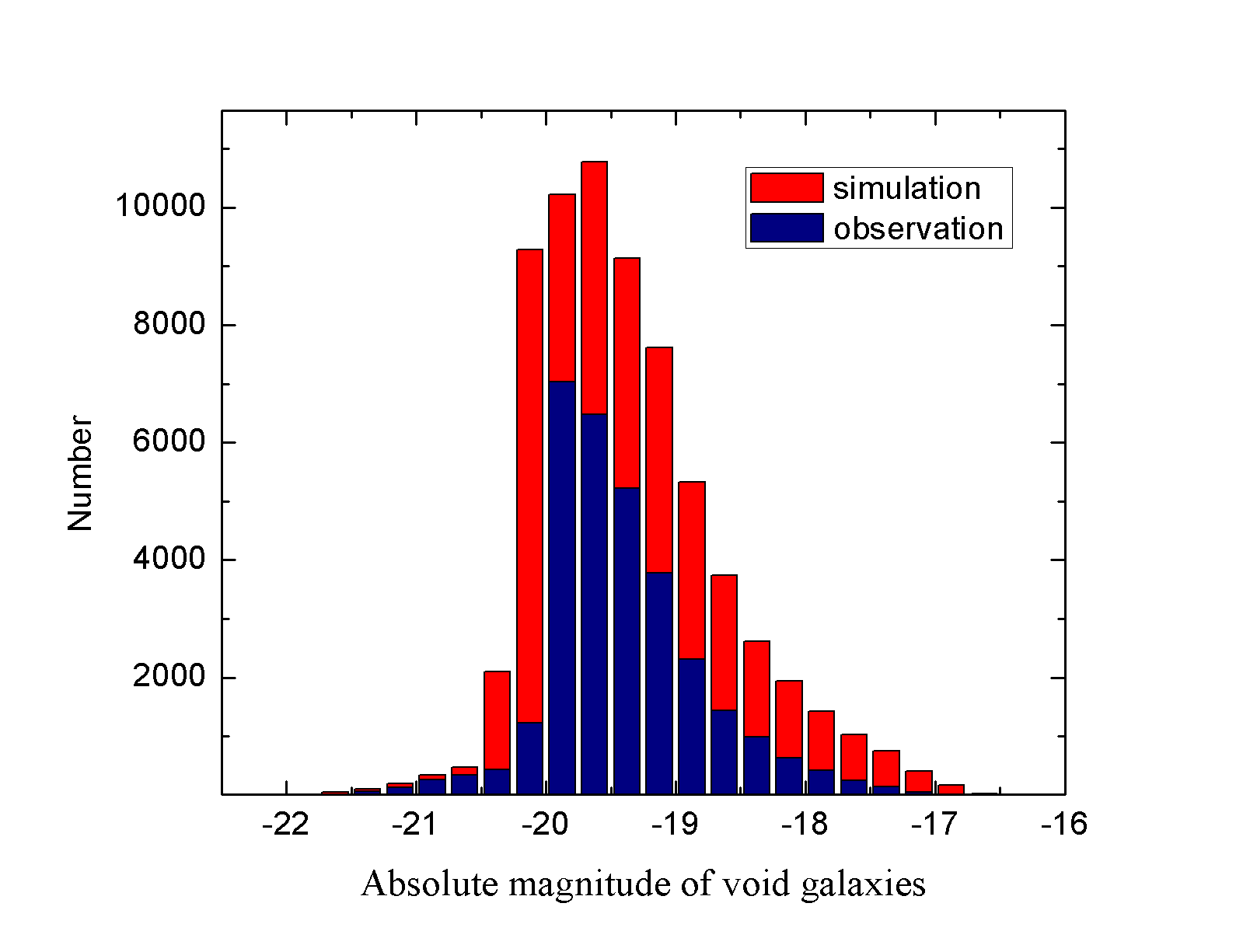
Figure 5: Number of void galaxies plotted against their absolute magnitudes. The luminosity range of void galaxies is nearly the same for the simulation and observation, which demonstrates that there is no bias imposed on the calculation of the void luminosities. Voids in the simulation contain more galaxies in almost all magnitude bands and hence are more luminous than those in the observation.

We comment that the void galaxies could be field galaxies or be field and faint galaxies. We recall that the field galaxies are in the luminosity ranges $M\textless-19.9$ in the observation and $M\textless-20.16$ in the simulation, but faint galaxies are less luminous than these thresholds set in our volume-limited sample (see Fig.5). We stress again that to obtain the same number density in both samples, we have to consider different luminosity thresholds in our two volume-limited samples (M=-19.9 & M=-20.16). The difference of luminosities is insignificant (about 0.26). Nonetheless, even if we consider the same luminosity threshold for both samples (e.g. M=-19.9), we derive the same result again and the galaxy luminosities in the simulation are higher than in the observation.

We compared the total luminosity of the voids and their luminosity per unit volume between the observation and the simulation. The comparisons are shown in Fig. 6. The lower panel of Fig. 6 shows that if we consider faint and field galaxies, large voids are clearly more luminous in the mock catalogue than in the observation. However, the top panel of Fig. 6 shows that if we consider only field galaxies, this discrepancy becomes less prominent. We emphasise that the lowest magnitude cut-off for both samples is nearly the same when faint galaxies are considered (see Fig.5). This discrepancy could be a sign of the over-abundance of small faint galaxies in the simulation. The problem of empty voids could be related to the lacking large power of $\Lambda$CDM, even though the value of $\sigma_{8}$ used here is $0.9$, which is higher than its present value of 0.8 given by WMAP7. Hence, this discrepancy is expected to be more significant for the WMAP7 value of $\sigma_{8}$.

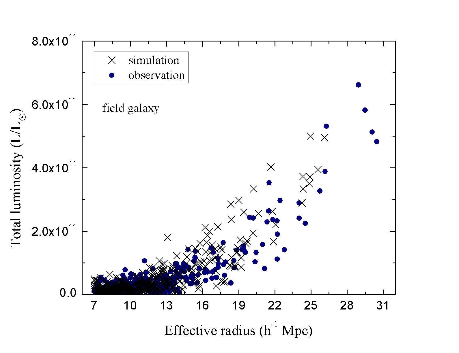
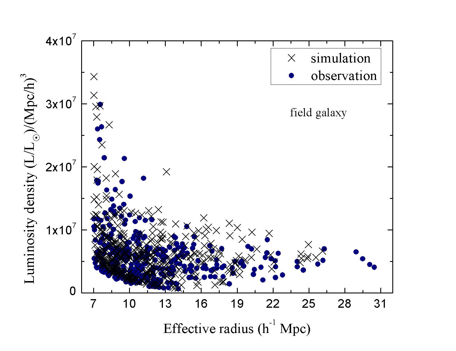
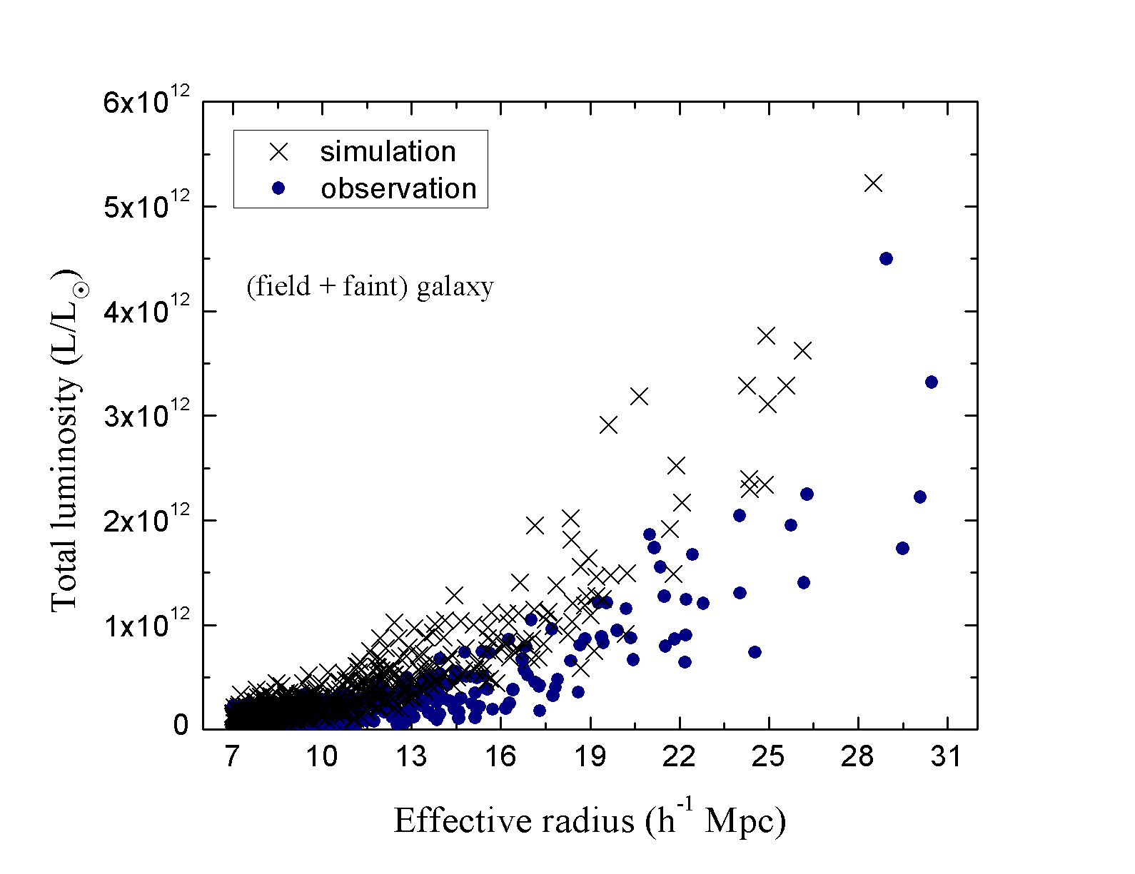
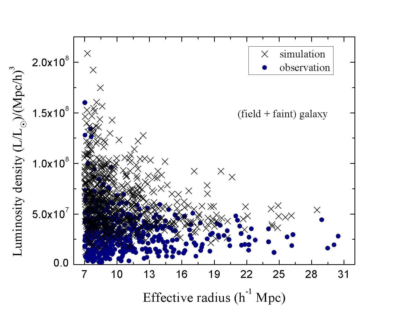
Figure 6: Top panel: total luminosity and luminosity density of field galaxies ploted against the effective radii of the voids to which they belong. Larger voids are less luminous in the observation than in the simulation. This disagreement becomes more significant when faint objects are also taken into account, as shown in the two plots of the lower panel. Observed voids are clearly less luminous than simulated voids. Note that the luminosity cutoffs are the same for the observation and the simulation when faint galaxies are taken into account. We expect this discrepancy to be even more significant than shown here because our Millennium I simulation uses a higher value of $\sigma_{8}$ than given by WMAP7.

8 Conclusion

We have carried out a parallel study of the voids in the SDSS DR7 redshift survey and in a mock catalogue. The latter was extracted from the Millennium I simulation and aims at replicating the observational biases and limitation of the SDSS DR7 catalogue.

We found that the total number and the volume occupied by the voids are larger in the simulation than in the observation. We found 467 voids in SDSS DR7 and 569 in the mock catalogue. The voids’ pseudo-radii or effective radii (i.e. radii of an equivalent spherical volume) range from 7 to 31 Mpc/h. The sphericities of voids also have similar distributions in the observation and the simulation. The voids also tend to become more spherical with increasing effective radii. Furthermore, large voids are less abundant in the simulation and the mean void luminosities, as defined by the sum of the luminosities of the galaxies they contain, is higher in the simulation. The aboundance problem of large voids could be related to the over-abundance problem of small haloes in $\Lambda$CDM ,which would then divide large voids into smaller ones in the simulation. However, this problem is usually taken care of in models of galaxy formation by suitable biasing or quenching of galaxy formation on small scales. The persistence of this problem could demonstrate that the semi-analytic model of galaxy formation used in the mock catalogue does not efficiently suppress galaxy formation in small voids. Recent catalogues of voids in SDSS including also the luminous red galaxies will be analysed in future works to obtain better statistics and shed more light on this problem (Sutter et al., 2012).

We also found that voids are in general more luminous in the simulation than in the observation. This could be related to the lack of power of $\Lambda$CDM on large scales. The value of $\sigma_{8}$ used in the Millennium I simulation is $0.9$ compared to the value of 0.8 given by the WMAP7. The problem of empty voids could then become even more significant if the current value of $\sigma_{8}$ were used in the simulation. Hence, either the ingredients used in the semi-analytic model do not correctly reproduce the observations, or on a more fundamental level, the power spectrum of $\Lambda$CDM has too much power on small scales and too little on large scales, which cannot be remedied by realistic models of galaxy formation.

Acknowledgments: We thank Sepehr Arbabi for collaborations and Habib Khosroshahi, Guilhem Lavaux, Gary Mamon, Joe Silk, and David Weinberg for discussions. RM thanks IPM and ST and KV thank IAP for their hospitality.

References

- Abazajian et al. (2009) Abazajian, K. N., Adelman-McCarthy, J. K., Agüeros, M. A., et al. 2009, ApJS, 182, 543
- Aikio & Maehoenen (1998) Aikio, J., & Maehoenen, P. 1998, ApJ, 497, 534
- Benson et al. (2003) Benson, A. J., Hoyle, F., Torres, F., & Vogeley, M. S. 2003, MNRAS, 340, 160
- Blaizot et al. (2005) Blaizot J., Wadadekar Y., Guiderdoni B., Colombi S. T., Bertin E., Bouchet, F. R., Devriendt, J. E. G., & Hatton, S. 2005, MNRAS, 360, 159
- Blanton & Roweis (2007) Blanton, M. R., & Roweis, S. 2007, AJ, 133, 734
- Blanton et.al. (2003a) Blanton M. R., Lin H., Lupton R. H., Maley F. M., Young N., Zehavi I., Loveday J., 2003a, AJ, 125, 2276
- Bothun et al. (1986) Bothun, G. D., Beers, T. C., Mould, J. R., & Huchra, J. P. 1986, ApJ, 308, 510
- Bower et al. (2012) Bower R. G., Benson A. J., & Crain, R. A., 2012, MNRAS, 422, 2816
- Bower et.al. (2006) Bower R. G., Benson A. J., Malbon R., Helly J. C., Frenk C. S., Baugh C. M., Cole S., & Lacey C. G., 2006, MNRAS, 370, 645
- Colberg et al. (2008) Colberg, J. M., Pearce, F., Foster, C., et al. 2008, MNRAS, 387, 933
- Copi et al. (2006) Copi, C. J., Huterer, D., Schwarz, D. J., & Starkman, G. D. 2006, MNRAS, 367, 79
- Davis et al. (1982) Davis, M., Huchra, J., Latham, D. W., & Tonry, J. 1982, ApJ, 253, 423
- da Costa et al. (1994) da Costa, L. N., Geller, M. J., Pellegrini, P. S., et al. 1994, ApJL, 424, L1
- da Costa et al. (1988) da Costa, L. N., Pellegrini, P. S., Sargent, W. L. W., et al. 1988, ApJ, 327, 544
- de Lapparent et al. (1986) de Lapparent, V., Geller, M. J., & Huchra, J. P. 1986, ApJL, 302, L1
- De Lucia & Blaizot (2007) De Lucia G., Blaizot J., 2007, MNRAS, 375, 2
- Efstathiou et al. (2010) Efstathiou, G., Ma, Y.-Z., & Hanson, D. 2010, MNRAS, 407, 2530
- Efstathiou (2004) Efstathiou, G. 2004, MNRAS, 348, 885
- Einasto et.al. (1980) Einasto J., Joeveer M., Saar E., 1980, MNRAS, 193, 353
- El-Ad & Piran (1997) El-Ad, H., & Piran, T. 1997, ApJ, 491, 421
- Geller & Huchra (1989) Geller, M. J., & Huchra, J. P. 1989, Science, 246, 897
- Goldberg et al. (2005) Goldberg, D. M., Jones, T. D., Hoyle, F., et al. 2005, ApJ, 621, 643
- Gottlöber et al. (2003) Gottlöber, S., Łokas, E. L., Klypin, A., & Hoffman, Y. 2003, MNRAS, 344,715
- Guo et al. (2011) Guo Q., White S., Boylan-Kolchin M., De Lucia G., Kauffmann G., Lemson G., Li C., Springel V., Weinmann S.,2011, MNRAS, 413, 101
- Hoeft et al. (2006) Hoeft, M., Yepes, G., Gottlöber, S., & Springel, V. 2006, MNRAS, 371, 401
- Hoyle et al. (2005) Hoyle, F., Rojas, R. R., Vogeley, M. S., & Brinkmann, J. 2005, ApJ, 620, 618
- Hoyle & Vogeley (2004) Hoyle, F., & Vogeley, M. S. 2004, ApJ, 607, 751
- Hoyle & Vogeley (2002) Hoyle, F., & Vogeley, M. S. 2002, ApJ, 566, 641
- Kauffmann & Fairall (1991) Kauffmann, G., & Fairall, A. P. 1991, MNRAS, 248, 313
- Kirshner et al. (1981) Kirshner, R. P., Oemler, A., Jr., Schechter, P. L., & Shectman, S. A. 1981, ApJL, 248, L57
- Klypin et.al. (1999) Klypin A., Kravtsov A. V., Valenzuela O., Prada F., 1999, ApJ, 522, 82
- Komatsu et.al. (2011) Komatsu E., Smith K. M., Dunkley J., Bennett C. L., Gold B., Hinshaw G., Jarosik N., Larson D., et al. 2011, ApJS, 192, 18
- Little & Weinberg (1994) Little, B., & Weinberg, D. H. 1994, MNRAS, 267, 605
- Menci et.al. (2012) Menci N., Fiore F., Lamastra A., 2012, MNRAS, 421, 2384M
- Moore et.al. (1999) Moore B., Ghigna S., Governato F., Lake G., Guinn T., Stadel J., Tozzi P., 1999, ApJ, 524, 19L
- Nusser et al. (2005) Nusser, A., Gubser, S. S., & Peebles, P. J. 2005, PRD, 71, 083505
- Pan et al. (2012) Pan, D. C., Vogeley, M. S., Hoyle, F., Choi, Y.-Y., & Park, C. 2012, MNRAS, 421, 926
- Patiri et al. (2006) Patiri, S. G., Prada, F., Holtzman, J., Klypin, A., & Betancort-Rijo, J. 2006, MNRAS, 372, 1710
- Peebles (2001) Peebles, P. J. E. 2001, ApJ, 557, 495
- Platen et al. (2008) Platen, E., van de Weygaert, R., & Jones, B. J. T. 2008, MNRAS, 387, 128
- Plionis & Basilakos (2002) Plionis, M., & Basilakos, S. 2002, MNRAS, 330, 399
- Rojas et al. (2004) Rojas, R. R., Vogeley, M. S., Hoyle, F., & Brinkmann, J. 2004, ApJ, 617, 50
- Ryden & Turner (1984) Ryden, B. S., & Turner, E. L. 1984, ApJL, 287, L59
- Sahni et al. (1994) Sahni, V., Sathyaprakah, B. S., & Shandarin, S. F. 1994, ApJ, 431, 20
- Schmidt et al. (2001) Schmidt, J. D., Ryden, B. S., & Melott, A. L. 2001, ApJ, 546, 609
- Shandarin et al. (2006) Shandarin, S., Feldman, H. A., Heitmann, K., & Habib, S. 2006, MNRAS, 367, 1629
- Shandarin & Zeldovich (1989) Shandarin, S. F., & Zeldovich, Y. B. 1989, Reviews of Modern Physics, 61, 185
- Springel et al. (2005) Springel V. et al., 2005, Nat, 435, 629
- Sutter et al. (2012) Sutter, P. M., Lavaux, G., Wandelt, B. D., & Weinberg, D. H. 2012, arXiv:1207.2524
- Tikhonov & Klypin (2009) Tikhonov, A. V., & Klypin, A. 2009, MNRAS, 395, 1915
- Tinker & Conroy (2009) Tinker, J. L., & Conroy, C. 2009, ApJ, 691, 633
- Tinker et al. (2008) Tinker, J. L., Conroy, C., Norberg, P., et al. 2008, ApJ, 686, 53
- Tully et al. (2008) Tully, R. B., Shaya, E. J., Karachentsev, I. D., et al. 2008, ApJ, 676, 184
- Wang et al. (2012) Wang, L., Weinmann, S. M. & Neistein, E., 2012, MNRAS, 421, 3450
- Zeldovich et al. (1982) Zeldovich, I. B., Einasto, J., & Shandarin, S. F. 1982, Nature, 300, 407