Superconductivity at the onset of spin-density-wave order in a metal

Abstract

We revisit the issue of superconductivity at the quantum-critical point (QCP) between a 2D paramagnet and a spin-density-wave metal with ordering momentum $(\pi,\pi)$. This problem is highly non-trivial because the system at criticality displays a non-Fermi liquid behavior and because the effective coupling constant $\lambda$ for the pairing is generally of order one, even when the actual interaction is smaller than fermionic bandwidth. Previous study [M. A. Metlitski, S. Sachdev, Phys.Rev.B 82, 075128 (2010)] has found that the renormalizations of the pairing vertex are stronger than in BCS theory and hold in powers of $\log^{2}(1/T)$, like in color superconductivity. We analyze the full gap equation and argue that, for QCP problem, summing up of the leading logarithms does not lead to a pairing instability. Yet, we show that superconductivity has no threshold and appears even if $\lambda$ is set to be small, because subleading logarithmical renormalizations diverge and give rise to BCS-like $\log(1/T_{c})\propto 1/\lambda$. We argue that the analogy with BCS is not accidental as at small $\lambda$ superconductivity at a QCP predominantly comes from fermions which retain Fermi liquid behavior at criticality. We compute $T_{c}$ for the actual $\lambda\sim O(1)$, and found that both Fermi-liquid and non-Fermi liquid fermions contribute to the pairing. The value of $T_{c}$ agrees well with the numerical results.

Introduction. Superconductivity at the onset of density-wave order in a metal is an issue of high current interest, with examples ranging from cuprates cuprates , to Fe-pnictides matsuda and other correlated materials cps ; chi ; rmp It is widely believed that the pairing in these systems is caused by repulsive electron-electron interaction, enhanced in a particular spin or charge channel, which becomes critical at the quantum-critical point (QCP). The pairing problem at QCP is highly non-trivial in $D\leq 3$, as scattering by a critical collective mode destroys Fermi liquid (FL) behavior above $T_{c}$ (Ref. nfl ; acs ). This is particularly relevant for systems near uniform density-wave instability (e.g., a ferromagnetic or a nematic one). In this case, FL behavior is lost on the whole Fermi-surface (FS), and superconductivity can be viewed as a pairing of incoherent fermions which exchange quanta of gapless collective bosons msv ; acf ; acs ; moon ; moon-sachdev . The pairing of incoherent fermions is qualitatively different from BCS/Eliashberg pairing of coherent fermions in a FL because in the incoherent case the pairing in $D<3$ occurs only if the interaction exceeds a certain threshold acf ; nick ; aace . For $D=3$ there is no threshold, but at small coupling constant $\lambda$, $\log{\Lambda/T_{c}}=1/\sqrt{\lambda}$ rather than $1/\lambda$ (Ref. joerg ), in close analogy to $T_{c}$ in color superconductivity (CSC) of quarks mediated by the exchange of gluons color

The non-FL behavior at criticality is less pronounced for systems near density-wave order at a finite momentum, because only fermions near particular points along the FS (hot spots) lose FL behavior at criticality. Still, fermions from hot regions mostly contribute to the pairing, and early studies of superconductivity at the onset of $(\pi,\pi)$ spin-density-wave (SDW) order acf ; acs placed the pairing problem into the same universality class as for QCP with $q=0$. The 2D problem has been recently re-analyzed ms by Metlitski and Sachdev (MS). They argued that it is important to include into the consideration the momentum dependence of the self-energy along the FS, neglected in earlier studies. Using the full form of $\Sigma(\omega_{m},{\bf k})$ for ${\bf k}$ on the FS, they found that the one-loop renormalization of the pairing vertex is larger than previously thought – it is $\log^{2}$ instead of $\log$, and that the enhancement comes from fermions somewhat away from hot spots, for which $\Sigma(\omega_{m},{\bf k})$ has a FL form at the smallest frequencies. The $\log^{2}$ behavior in the perturbation theory holds for CSC, and MS result raises the question whether the pairing problem at a 2D SDW QCP is in the same universality class as CSC. The related issues raised by MS work are: (i) is the problem analogous to the pairing at a 2D SDW QCP a FL phenomenon, or non-FL physics is essential, (ii) what sets the scale of $T_{c}$, and (iii) is $T_{c}$ non-zero only if the coupling $\lambda$ exceed a finite threshold, as it happens if one approximates $\Sigma(\omega_{m},{\bf k})$ by $\Sigma(\omega_{m})$ at a hot spot, or $T_{c}$ is non-zero even at smallest $\lambda$, like in CSC?

In this letter, we address these issues. We first show that the analogy with CSC does not extend beyond one-loop order, and in our case the summation of $\log^{2}$ terms in the Cooper channel does not give rise to a pairing instability. However, that subleading $\log$ terms do give rise to a pairing instability, and at weak coupling yield $\log\Lambda/T_{c}\propto 1/\lambda$, like in BCS theory. We show that the analogy with BCS formula is not accidental because the pairing at small $\lambda$ predominantly comes from fermions for which fermionic self-energy has a FL form. We then analyze the physical case $\lambda=O(1)$ and argue that in this case fermions from both FL and non-FL regimes contribute to the pairing and that $T_{c}\approx 0.04\omega_{0}$, where $\omega_{0}$ is the frequency at which $\Sigma(\omega_{m})$ at a hot spot becomes equal to $\omega_{m}$. The numerical prefactor agrees with the slope of $T_{c}$ obtained by solving the gap equation numerically along the full FS acn .

The model.     We follow earlier worksacf ; acs ; ms and analyze the pairing near an antiferromagnetic QCP within the semi-phenomenological spin-fermion model. The model assumes that antiferromagnetic correlations develop already at high energies, of order bandwidth, and mediate interactions between low-energy fermions. The static part of the spin-fluctuation propagator is treated as a phenomenological input from high-energy physics, but the the dynamical Landau damping part is self-consistently obtained within the model as it comes entirely from low-energy fermions acf ; acs ; ms . In the Supplementary material we review justifications for the spin-fermion model and compare spin-fermion approach with the RG-based approaches rg ; rg_1 ; rg_2 ; rg_3 which treat superconductivity, magnetism, and specific charge density-wave orders on equal footings.

We assume, like in acf ; acs ; ms , that fermions have $N\gg 1$ flavors and that collective spin excitations are peaked at ${\bf Q}=(\pi,\pi)$, and focus on the hot regions on the FS, i.e., on momenta near ${\bf k}_{F}$, for which ${\bf k}_{F}+{\bf Q}$ is also near the FS. The Lagrangian of the model is given by cps ; acs ; ms

$${\mathcal{S}} = -\int_{k}^{\Lambda}G_{0}^{-1}\left(k\right)\psi_{k,\alpha}^{\dagger}\psi_{k,\alpha}+\frac{1}{2}\int_{q}^{\Lambda}\chi_{0}^{-1}\left(q\right)\ {\bf{S}}_{q}\cdot{\bf{S}}_{-q}$$ (1)

$$+g\int_{k,q}^{\Lambda}\psi_{k+q,\alpha}^{\dagger}\sigma_{\alpha\beta}\psi_{k,\beta}\cdot{\bf{S}}_{-q}.\$$

where $\int_{k}^{\Lambda}$ stands for the integral over $d-$dimensional ${\bf{k}}$ (up to some upper cutoff $\Lambda$) and the sum over fermionic and bosonic Matsubara frequencies, $G_{0}\left(k\right)=G_{0}(\omega_{m},{\bf k})=1/[i\omega_{m}-{\bf v}_{F,{\bf k}}({\bf k}-{\bf k}_{F})]$ is the bare fermion propagator, and $\chi_{0}\left(q\right)=\chi_{0}(\Omega_{m},{\bf q})=\chi_{0}/({\bf q}^{2}+\xi^{-2})$ is the static propagator of collective bosons, in which $\xi^{-1}$ measures a distance to a QCP and ${\bf q}$ is measured with respect to ${\bf Q}$. We set $\xi^{-1}=0$ below. The fermion-boson coupling $g$ and $\chi_{0}$ appear in theory only in combination ${\bar{g}}=g^{2}\chi_{0}$ and we will use ${\bar{g}}$ below. The Fermi velocities at hot spots separated by ${\bf Q}$ can be expressed as ${\bf v}_{F,1}=(v_{x},v_{y})$ and ${\bf v}_{F,2}=(-v_{x},v_{y})$, where $x$ axis is along ${\bf Q}$. We will also use $\alpha=v_{y}/v_{x}$ and $v_{F}=(v^{2}_{x}+v^{2}_{y})^{1/2}$. The model of Eq. (1) can be equivalently viewed as a four-patch model for fermions near hot spots at $\pm{\bf k}_{F}$ and $\pm({\bf k}_{F}+{\bf Q})$ (Ref. ms ; ms_1 ). The hot spot model is obviously justified only when the interaction ${\bar{g}}$ is smaller than $E_{F}$.

The fermion-boson coupling gives rise to fermionic and bosonic self-energies. In the normal state, bosonic self-energy accounts for Landau damping of spin excitations, while fermionic self-energy accounts for the mass renormalization and a finite lifetime of a fermion. At one-loop level, self-consistent normal-state analysis yields acs ; ms ; millis

$$\chi(\Omega_{m},{\bf q})=\frac{\chi_{0}}{{\bf q}^{2}+|\Omega_{m}|\gamma}$$ (2)

$$\Sigma(\omega_{m},k_{\parallel})=\frac{3{\bar{g}}}{4\pi v_{F}}~{}\frac{2\omega_{m}}{\sqrt{\gamma|\omega_{m}|+\left(\frac{2k_{\parallel}\alpha}{1+\alpha^{2}}\right)^{2}}+\left|\frac{2k_{\parallel}\alpha}{1+\alpha^{2}}\right|},$$ (3)

where $\gamma=2N{\bar{g}}/(\pi v_{x}v_{y})$ and $k_{\parallel}$ is a deviation from a hot spot along the FS. The bosonic propagator $\chi(\Omega_{m},{\bf q})$ describes Landau-overdamped spin fluctuations. The fermionic self-energy has a non-FL form right at a hot spot: $\Sigma(\omega_{m},0)=(|\omega_{m}|\omega_{0})^{1/2}{\rm sgn}\omega_{m}$, where $\omega_{0}=(9{\bar{g}}/(16\pi N))(2v_{x}v_{y}/v^{2}_{F})$. Away from a hot spot, $\Sigma(\omega_{m},k_{\parallel})$ retains a FL form at the smallest $\omega_{m}$ and scales as $\Sigma(\omega_{m},k_{\parallel})\propto\omega_{m}/|k_{\parallel}|$.

We use Eqs. 2 and 3 as inputs for the pairing problem and neglect higher order terms in the loop expansion. Most of higher-order terms are small in $1/N$, but some terms with $n\geq 4$ loops do not contain $1/N$ (Refs. ms ; sslee ; ms_1 ). The terms without $1/N$ include, in particular, feedback effects from pairing fluctuations on the fermionic and bosonic propagators. We verified that these feedback effects preserve the forms of $\chi$ and $\Sigma$, and we just assume that they do not substantially modify the prefactors.

The pairing vertex     We add to the action the anomalous term $\Phi_{0}(k)\psi_{k,\alpha}(i\sigma^{y})_{\alpha\beta}\psi_{-k,\beta}$ and use Eq. (1) to renormalize it into the full $\Phi(k)$. At $T_{c}$, the pairing susceptibility $\chi_{pp}(k)=\Phi(k)/\Phi_{0}$ must diverge for all $k$. The bare $\Phi_{0}$ can be set constant within a patch, but has to change signs between patches separated by ${\bf Q}$ (the pairing symmetry at the onset of SDW order is a $d-$wave Scal ). The one-loop renormalization of $\Phi(k)$ at $k=(\omega\sim T,0)$ was obtained by MS:

$$\Phi(\omega\sim T,0)=\Phi_{0}\left(1+\frac{\lambda}{2\pi}\log^{2}{\Lambda/T}\right),~{}~{}\lambda=\frac{2\alpha}{(1+\alpha^{2})},$$ (4)

where $\Lambda$ is the smaller of $\omega_{0}$ and $\alpha^{4}E_{F}^{2}/\omega_{0}$. Notice that neither the coupling constant ${\bar{g}}$ not $1/N$ appear in (4), the only parameter is the ratio of the velocities $\alpha$, which is a geometrical property of the FS. For a cuprate-like FS, $\alpha\sim 1$, i.e., the pairing coupling constant $\lambda=O(1)$. To understand the physics of the pairing at the QCP, we find that it is instructive to formally replace $\lambda$ by $\varepsilon\lambda$ and first analyze the pairing in the “weak coupling” case $\varepsilon\ll 1$.

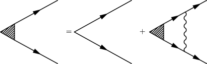
Figure 1: Diagrammatic representation for the pairing vertex. The shaded triangle is the full $\Phi_{k}$, the unshaded vertex is the bare $\Phi_{0}$, solid lines are full fermionic propagators, and the wavy line is the Landau-overdamped spin propagator. The pairing vertex contains $i\sigma^{y}_{\alpha,\beta}$, the vertices where wavy and solid lines meet contain ${\bf\sigma}_{\gamma\delta}$.

Let’s first see where $\log^{2}$ renormalization comes from. The one-loop diagram for $\Phi$ contains two fermionic propagators $G(k)$ and $G(-k)$ and one bosonic $\chi(k)$ (Fig.1). Large $N$ allows one to restrict $\chi(\Omega_{m},{\bf k})$ to momenta connecting points at the FS and integrate over momenta transverse to the FS in the fermionic propagators only. Because $\Sigma$ does not depend on this momentum, the integration is straightforward, and yields, to logarithmic accuracy $\int GG\chi\propto\int dk_{\parallel}\int_{T}d\Omega_{m}(\chi(\Omega_{m},k_{\parallel})/|\Omega_{m}+\Sigma(\Omega_{m},k_{\parallel}))|$. At $k^{2}_{\parallel}>\gamma\Omega_{m}$ and $|k_{\parallel}|<k_{F}{\bar{g}}/v_{F}$, $1/|\Omega_{m}+\Sigma(\Omega_{m},k_{\parallel})|$ scales as $|k_{\parallel}/\Omega_{m}|$ and $\chi(\Omega_{m},k_{\parallel})\propto 1/k^{2}_{\parallel}$. Integrating over $k_{\parallel}$ we obtain $\int_{\gamma|\Omega_{m}|}dk^{2}_{\parallel}/k^{2}_{\parallel}\propto\log|\Omega_{m}|$, and the remaining integral over frequency yields $\int GG\chi\propto\int_{T}(d\Omega_{m}/|\Omega_{m}|)~{}\log{|\Omega_{m}|}\propto\log^{2}T$. We see that the $\log^{2}T$ dependence originates from extra logarithm from $k-$integration. This extra logarithm is in turn the consequence of $\Omega_{m}/k_{\parallel}$ form of self-energy $\Sigma(\Omega_{m},k_{\parallel})$ at $k^{2}_{\parallel}>\gamma\Omega_{m}$. As $\Sigma\propto\omega$ is the property of a FL, the $\log^{2}T$ renormalization comes from fermions which preserve a FL behavior at a QCP. We further see that the one-loop renormalization can be interpreted as coming from the process in which fermions are exchanging quanta of an effective local $\log\Omega$ interaction. The same process determines one-loop renormalization of $\Phi$ in CSC.

The $\log^{2}$ analysis can be extended beyond leading order. We assume that $\lambda=2\varepsilon\alpha/(1+\alpha^{2})$ is small (because we set $\varepsilon$ to be small), but $\lambda\log^{2}T=O(1)$, and sum up ladder series of $\lambda\log^{2}T$ terms, neglecting smaller powers of logarithms at each order of loop expansion. Performing the calculations (see Supplementary material for details), we find that the analogy with CSC does not extend beyond leading order: for CSC the summation of $\lambda\log^{2}T$ terms yields $\Phi=\Phi_{0}/\cos[(2\lambda\log^{2}T)^{1/2}]$ (Ref.joerg ), and the system develops a pairing instability at $|\log T_{c}|=\pi/2\sqrt{2\lambda}$ (Ref. color ). In our case, perturbation series yield $\Phi=\Phi_{0}e^{\lambda/2\pi\log^{2}T}$, i.e., the pairing susceptibility increases with decreasing $T$, but never diverges. Because the summation of the leading logarithms does not lead to a finite $T_{c}$, one has to go beyond the leading logarithmical approximation and analyze the full equation for $\Phi(k)$ at $\Phi_{0}=0$ in order to understand whether or not $T_{c}$ is finite at a QCP. This is what we do next.

$\begin{array}[]{cc}\includegraphics[width=130.08731pt]{fig_2a.eps}&\includegraphics[width=130.08731pt]{fig_2b.eps}\end{array}$

Figure 2: Numerical solution of Eq. (6) at small $\varepsilon$. (a) The transition temperature. When $\varepsilon$ decreases, $\varepsilon\log\omega_{0}/T_{c}$ approaches $1$, as in Eq. (8). (b) The eigenfunction $\Phi(y)$, where $y=k^{2}_{\parallel}/(\pi T\gamma)$. Solid and dashed lines are numerical and analytical solutions of Eq. 6, respectively. The two are very close, except for the largest $y\sim\omega_{0}/T$, when the cutoff becomes relevant.

Full gap equation.    Within our approximation, the full linearized equation for the anomalous vertex is obtained by summing up ladder diagrams and keeping the self-energy in the fermionic propagator. Integrating the r.h.s. of this equation over momenta transverse to the FS, we obtain

$$\Phi(\omega_{m},k_{\parallel})=\frac{3{\bar{g}}}{2v_{F}}T\sum_{m^{\prime}}\int\frac{dk^{\prime}_{\parallel}}{2\pi}\frac{\Phi(\omega_{m^{\prime}},k^{{}^{\prime}}_{\parallel})}{|\omega_{m^{\prime}}+\Sigma(\omega_{m^{\prime}},k^{{}^{\prime}}_{\parallel})|}$$

$$\times\frac{1}{k^{2}_{\parallel}+k^{{}^{\prime}2}_{\parallel}-2\mu k_{\parallel}k^{{}^{\prime}}_{\parallel}+\gamma|\omega_{m}-\omega_{m^{{}^{\prime}}}|}$$ (5)

where $\mu=(1-\alpha^{2})/(1+\alpha^{2})$. The temperature at which the solution exists is $T_{c}$. The overall factor ${3\bar{g}}/(2v_{F})$ is eliminated by rescaling and get replaced by $\lambda$, which, we recall, we treat as a small parameter. One can verify that typical $k^{2}_{\parallel}$ are larger than typical $\gamma\omega_{m}$, and that the vertex $\Phi(\omega_{m},k_{\parallel})$ has a stronger dependence on $k_{\parallel}$ than on frequency. In this situation, one can approximate $\Phi(\omega_{m},k_{\parallel})$ by $\Phi(k_{\parallel})$, explicitly sum up over frequency and reduce (5) to 1D integral equation.

For simplicity, we first consider the case when $\alpha=1$, i.e $\lambda=\varepsilon$. Introducing ${\bar{T}}=\pi T/\omega_{0}$ and $x=k^{2}_{\parallel}/(\gamma\omega_{0}{\bar{T}})$, we obtain from (5)

$$\Phi(y)=\frac{\varepsilon}{\pi}\int_{1}\frac{dx}{x+y}\frac{\log{x}}{2\sqrt{x{\bar{T}}}+1}\Phi(x)$$ (6)

The term in the denominator with $\sqrt{x{\bar{T}}}$ is a soft upper cutoff.

The r.h.s. of (6) contains $\log^{2}$ contributions from the range $x\gg y$, but, as we just found, they do not lead to a pairing instability. We therefore focus on the contribution from $x\sim y$. Because the kernel is logarithmical, we search for $\Phi(x)$ in the form $\Phi(x)=\exp[-f(p(x))]$, where $p(x)=\varepsilon\log{x}$. Substituting this into (6), we find that the form is reproduced at $1\ll x\ll 1/{\bar{T}}$, when soft cutoff can be omitted. The self-consistency condition yields (see Supplementary material)

$$f(z)=\frac{1}{\pi\varepsilon}\left(z\arcsin{z}+\sqrt{1-z^{2}}-1\right).$$ (7)

At small $\varepsilon$, the soft cutoff can be replaced by the boundary condition that $df(z)/dz$ must be at a maximum at $z=\varepsilon|\log{\bar{T}}|$. This condition sets

$$T_{c}\sim\omega_{0}e^{-1/\varepsilon}.$$ (8)

To verify this reasoning, we solved Eq. (6) numerically and found very good agreement with analytical results (see Fig.2).

We next analyze the gap equation at $\alpha\neq 1$ Using the same logic as before we find (see Supplementary material for details) that Eq. (8) does not change, i.e., to logarithmical accuracy, $T_{c}/\omega_{0}$ does not depend on the angle between Fermi velocities at ${\bf k}_{F}$ and ${\bf k}+{\bf Q}$. We verified the independence of $T_{c}/\omega_{0}$ on $\alpha$ by solving Eq. (6) numerically for different $\alpha$.

We see from (8) that $T_{c}$ is non-zero already at infinitesimally small coupling, like in BCS theory. The analogy is not accidental as the pairing predominantly comes from momenta away from hot spots, for which $x\sim y\sim{\bar{T}}$, i.e., $k_{\parallel}\sim k_{\perp}\sim(\gamma\omega_{0})^{1/2}$. Because $T_{c}\ll\omega_{0}$, typical $\gamma\omega\geq\gamma T_{c}$ are much smaller than $\gamma\omega_{0}$, hence fermionic self-energy for $k_{\parallel}\sim(\gamma\omega_{0})^{1/2}$ has the FL form $\Sigma(\omega_{m},k_{\parallel})\propto\omega_{m}/|k_{\parallel}|$. Furthermore, for $x\sim y$ in (6), the integration over $x$ does not give rise to an additional logarithm besides $\log x$, which is a Cooper logarithm. The instability at $T_{c}$ is then a conventional Cooper instability of a FL with a weak and non-singular attractive coupling $\varepsilon$. In other words, for small $\varepsilon$, the pairing at a SDW QCP is entirely a FL phenomenon.

Although Eq. (8) looks like BCS formula, the problem we are solving is not a weak-coupling pairing by a static attractive interaction. We emphasize in this regard that a non-zero $T_{c}$ at small $\varepsilon$ is the consequence of the dependence of the self-energy on the momenta along the FS. Earlier works acf ; acs neglected this momentum dependence and approximated the self-energy by its non-FL form $\Sigma(\omega)=\omega_{m}(\omega_{0}/|\omega_{m}|)^{1/2}$ at a hot spot. These studies found a different result: $T_{c}$ at an AFM QCP becomes non-zero only if $\varepsilon$ exceeds a certain threshold, like in the pairing problem at a QCP with $q=0$ (Refs.aace ; max_last ). Specifically, for $\Sigma=\Sigma(\omega_{m})$, the anomalous vertex $\Phi$ also depends only on frequency, and Eq. (5) reduces to 1D integral equation in frequency rather than in momentum:

$$\Phi(\omega_{m})=\frac{\pi\varepsilon T}{2}\sum_{m^{\prime}\neq m}\frac{\Phi(\omega_{m^{\prime}})}{\sqrt{|\omega_{m^{\prime}}|}Z_{\omega_{m^{\prime}}}\sqrt{|\omega_{m}-\omega_{m^{\prime}}|}}.$$ (9)

where $Z_{\omega_{m^{\prime}}}=1+\sqrt{|\omega_{m^{\prime}}|/\omega_{0}}$. This equation has been solved for arbitrary ${\varepsilon}$  acf , and the result is that $T_{c}$ becomes non-zero only when ${\varepsilon}$ exceeds a critical value ${\varepsilon}_{c}=0.22$. Near critical coupling $T_{c}\sim\omega_{0}e^{-3.41/({\varepsilon}-{\varepsilon}_{c})^{1/2}}$, and for ${\varepsilon}=1$, $T_{c}=0.17\omega_{0}$.

$T_{c}$ at moderate coupling.     For the actual physical case $\varepsilon=1$ we solved Eq. 5 numerically and found that the behavior of $T_{c}(\alpha)$ is very similar to that at small $\varepsilon$. Namely, $T_{c}$ scales with $\omega_{0}$ and the prefactor is essentially independent on $\alpha$ as long as $\alpha\gg{\bar{g}}/E_{F}$. We obtained

$$T_{c}\approx 0.04\omega_{0}.$$ (10)

For $\varepsilon=1$, typical $(\alpha k_{\parallel})^{2}\sim\gamma\omega_{0}$ and typical $\gamma\omega\sim\gamma T_{c}$ are now comparable, i.e., for $\varepsilon=1$ the pairing comes from fermions whose self-energy is in a grey area between a FL and a non-FL. We checked this by solving for $T_{c}$ using the two limiting forms of the self-energy in Eq. (2) – the non-Fl $\Sigma(\omega_{m})$ right at a hot spot (this gives $T_{c}\sim 0.17\omega_{0}$) and the FL form $\Sigma(\omega_{m},k_{\parallel})\propto\omega_{m}/k_{\parallel}$ (this gives $T_{c}=0.005\omega_{0}$). The actual $T_{c}$ given by Eq. (10) is in between the two limits. We also verified (see Supplementary material) that in the extreme case of strong nesting, when $\alpha$ gets smaller than $({\bar{g}}/E_{F})$, the momentum dependence of the self-energy becomes irrelevant for all $k_{\parallel}$ along the FS, and $T_{c}$ crosses over to $T_{c}\sim 0.17\omega_{0}$.

The linearized gap equation has been previously solved numerically along the full FS, without restriction to hot spots acn . In notations of Ref.  acn , $T_{c}=(v_{F}/a)f(u)$, where dimensionless $u=4\omega_{0}a/(3v_{F})$. Eq. (10) implies that $f(u)=0.03u$ at small $u$. This agrees well with the numerical solution in acn . At larger $u\geq 1/2$, $f(u)$ saturates at around $0.015-0.02$ (Refs. acn, ; numerics, ), and at larger $u$ decreases as $1/u$ because of Mott physics.

Conclusions.    In this paper we analyzed the equation for superconducting $T_{c}$ at the onset of SDW order in a 2D metal. We demonstrated that the leading perturbation correction to the bare pairing vertex contains $\log^{2}T$, but the series of $\log^{2}T$ renormalizations do not give rise to the pairing instability. Yet, $T_{c}$ is finite, even when coupling $\lambda$ is artificially set to be small, because of subleading, $\log T$ terms. We showed that for physical $\lambda=O(1)$, the pairing at a QCP comes from fermions with both FL and non-FL forms of the self-energy. The overall scale of $T_{c}$ is set by the interaction ($\omega_{0}\sim{\bar{g}}$), as long as the interaction is smaller than the Fermi energy, and the prefactor is essentially independent on the details of the geometry of the FS.

The issue which requires a further study is how robust these results are with respect to feedback effects from pairing fluctuations on the fermionic and bosonic propagators. These feedbacks are quite relevant in the RG-based studies rg ; rg_1 ; rg_2 ; rg_3 . In the spin-fermion model, the corrections from the pairing channel come from diagrams with $n\geq 4$ loops and are not small in $1/N$. These corrections preserve the Landau-overdamped form of the bosonic propagator and the $\omega/k_{\parallel}$ form of the fermionic self-energy, but may contribute additional logarithm $\log{k^{2}_{\parallel}/(\gamma|\omega|)}$ to $\Sigma$ (see Ref. ms_1 and Supplementary material). The argument of the logarithm is, however, of order one for typical $k_{\parallel}$ and $\omega$ in the calculations of $T_{c}$, hence we expect that the feedbacks from the pairing channel will at most change the prefactor for $T_{c}$ but do not change our two main conclusions that (i) $T_{c}$ scales with $\omega_{0}$, and (ii) in the physical case the pairing involves fermions with both FL and non-FL forms of the self-energy. It is very likely that the same conclusions can be reached within RG-based approaches as the results of the RG analysis are generally comparable to those obtained in the spin-fermion model rg_3 .

We acknowledge stimulating discussions with Y.B. Kim, S.S. Lee, M.A. Metlitski, S. Sachdev, T. Senthil, and A-M Tremblay. The research has been supported by DOE DE-FG02-ER46900.

I Supplementary Material

II Spin-fermion model and its relation to RG-based theories

For a generic metal with no nesting of the Fermi surface, an instability towards a magnetic order does not occur at weak coupling, but may occur when the interaction $U$ becomes of order of fermionic bandwidth, $W$. In this intermediate coupling regime, exact analytical treatment is hardly possible and one has to rely on approximate computational schemes in a hope that an approximate treatment still captures the key physics of the underlying microscopic model. The spin-fermion model is a “minimal” semi-phenomenological effective low-energy model of this kind. It takes as inputs the experimental Fermi surface and the experimental fact that the underlying system does have a transition between a metallic paramagnet and a metallic antiferromagnet (often called a spin-density-wave (SDW)). Since Fermi surface shows no nesting, the underlying interaction must be of order bandwidth, which in turn implies that antiferromagnetic correlations come from fermions with energies comparable to the bandwidth. The spin-fermion model is applicable if antiferromagnetism is the only instability which develops already at energies comparable to a bandwidth. There may be other instabilities (e.g., superconductivity or charge order), but the assumption is that they develop at energies smaller than the upper end set for the spin-fermion model and can be fully understood within the low-energy theory.

The Lagrangian of the spin-fermion model (Eq. (1) in the main text) contains three terms describing fermions, collective spin excitations, and the minimal coupling between a spin of a fermion and a spin of a collective excitation. Such a Lagrangian can be formally derived within RPA, starting from a Hubbard model cm1 , but this only serves an illustration purpose because RPA is an uncontrolled approximation for $U\sim W$. A more sophisticated justification of the spin-fermion model with respect to, e.g., the Hubdard model near optimal doping, comes from numerical studies scalapino1 in which the pairing interaction and the dynamical spin susceptibility were calculated independently and, to a good accuracy, were found to be proportional to each other.

The description within the low-energy spin-fermion model makes sense if the interaction does not mix low-energy and high-energy sectors. This is true if the residual interaction between low-energy fermions (${\bar{g}}$ in the notations of the main text) is smaller than the upper energy cutoff of the theory, which is generally a fraction of the bandwidth. At a face value, such an approximation is not consistent with the initial assumption that the underlying, microscopic interaction $U$ is of order bandwidth. There are several ways to make the assumptions ${\bar{g}}\ll W$ and $U\sim W$ consistent cm1 (e.g., if microscopic interaction has a length $a$ which is large enough such that $ak_{F}\gg 1$, ${\bar{g}}$ is small in $1/(ak_{F})$ compared to $U$). But since the properties of spin-fermion model do not depend in any singular way on ${\bar{g}}/W$ ratio, the hope is that, even for a short-range interaction, spin-fermion model captures the essential physics of the system behavior near an antiferromagnetic instability in a metal, including a pre-emptive superconducting instability.

Several authors rg1 ; rg_11 ; rg_21 ; rg_31 put forward another approach, which employs the renormalization group (RG) technique. This approach assumes that interactions in all channels, including the SDW one, are small at energies of order bandwidth, but evolve as one progressively integrates out high-energy degrees of freedom. This approach departs directly from the underlying microscopic model and treats superconductivity, SDW, and specific charge-density-wave instabilities on equal footings. From this perspective, it is more microscopic and less biased than spin-fermion model. At the same time, the RG approach has its own limitation because it assumes that that the tendency towards a SDW order can be detected already at a weak coupling. This is true if the Fermi surface is nested and the bare SDW susceptibility at an antiferromagnetic momentum is logarithmically enhanced. Then one can rigorously separate logarithmical and non-logarithmical vertex renormalizations, neglect non-logarithmical ones, derive the set of coupled RG equations for different vertices, and analyze the interplay between different ordering tendencies. Examples when the SDW susceptibility is logarithmically enhanced include cuprates and graphene near van-Hove doping rg1 , Fe-pnictides rg_11 , and quasi-1D organic conductors rg_21 .

Figure 3: The self-energy renormalization from fluctuations in the pairing channel. The lowest order in the series is a part of one-loop self-energy, the new diagrams appear at 4-loop and higher order. These diagrams are not small in $1/N$ and are of the same order as the one-loop self-energy. These diagrams can only be neglected by numerical reasons.

Figure 4: The two-loop self-energy diagram with vertex correction. This diagram is small by $1/N$ compared to one-loop diagram.

For a generic non-nested Fermi surface, a bare SDW susceptibility is, however, not enhanced and generally is of order of inverse bandwidth $1/W$. Then one needs large $U\sim W$ to bring the system to the vicinity of an SDW instability, and the terms neglected in the RG scheme become of order one. Whether to use spin-fermion model or RG technique in this situation becomes a somewhat subjective issue. Our justification of using the spin-fermion model for a 2D metal with cuprate-like Fermi surface is based on a’posteriori argument that superconducting $T_{c}\approx 0.04{\omega_{0}}$ is numerically much smaller than the scale $\omega_{0}$, below which antiferromagnetic correlations substantially modify fermionic self-energy. The smallness of $T_{c}/\omega_{0}$ then implies that there exists a wide range of energies in which magnetic correlations strongly modify self-energy, yet superconducting fluctuations are still weak. This was our motivation to compute first fermionic self-energy due to spin fluctuation exchange and then use it as an input for the calculation of $T_{c}$. If $T_{c}$ and ${\omega_{0}}$ were comparable, one could not separate SDW and superconducting channels and had to treat them on equal footing.

II.1 pairing fluctuations in the spin-fermion model

A more subtle issue is whether pairing fluctuations can be rigorously neglected in the spin-fermion model, at least in the limit of large number of fermionic flavors, $N$. We checked this and argue that the corrections from pairing fluctuations are not small in $1/N$ and can be neglected only by numerical reasons. In this respect, the corrections from pairing fluctuations are different from ordinary vertex corrections, as the latter are small in $1/N$. Our consideration closely follows the one by Hartnoll et al ms_11 who found that $2k_{F}$ scattering gives rise to self-energy corrections which are not small in $1/N$.

The self-energy due to pairing fluctuations is presented in Fig. 3. The double wavy line represents a series of diagrams which contain pairs of fermions with near-opposite frequencies and momenta. The diagrams contain even number of bosonic propagators, otherwise one would need to include at least one interaction with a small momentum transfer. The lowest diagram with two propagators is already included into the one-loop self-energy considered in the main text (the extra bubble gives rise to Landau damping term). At a hot spot, it yields $\Sigma^{(1)}(\omega)\propto({\bar{g}}\omega/N)^{1/2}$ (the notations are the same as in the main text). The next in series is the diagram with $n=4$ loops. It contains four bosonic propagators, seven fermionic Green’s functions, and the integration is over four intermediate 2D momenta and four frequencies. Fermions in the seven Green’s functions are combined into three pairs in the particle-particle channel and one unpaired fermions. Integrations transverse to the Fermi surface then involve four momentum components. Three integrals involving pairs of fermionic Green’s functions yield $1/(v_{F}\Sigma^{(1)}(\omega^{\prime}))^{3}$, where $\omega^{\prime}$ is one of four internal frequencies, which are all of the same order, the fourth integration gives additional $1/v_{F}$ and restricts internal frequencies to be of order on external $\omega$. Integration over the other four momentum components involves four fermionic propagators and yields $1/(\gamma\omega^{\prime})^{2}$. The total four-loop self-energy at a hot spot is then

$$\Sigma^{(4)}(\omega)\propto\left(\frac{\bar{g}}{v_{F}}\right)^{4}\frac{\omega^{4}}{(\gamma\omega)^{2}(\Sigma^{(1)}(\omega))^{3}}$$ (11)

Using $\gamma\sim{\bar{g}}N/v^{2}_{F}$ we find that $\Sigma^{(4)}(\omega)\propto({\bar{g}}\omega/N)^{1/2}$ is of the same order as $\Sigma^{(1)}(\omega)$, i.e., additional loop order does not give rise to additional powers of $1/N$. One can easily make sure that this holds for all higher order diagrams with $n=6$, $n=8$, etc loops.

It is instructive to compare this behavior with the effect of a vertex correction. The two-loop self-energy diagram of this kind is shown in Fig. 4. It contains three fermionic and two bosonic propagators and integrals over two internal 2D momenta and two frequencies. The distinction from the previous case is that now one needs three components of momenta to integrate over three fermionic dispersions. These three integrals yield $1/(v_{F})^{3}$ and restrict internal frequencies to be of order of external $\omega$. The remaining momentum integral involves one bosonic propagator and yields $1/(\gamma\omega)^{1/2}$. This leaves one bosonic propagator and two frequency integrals. the integration yields $\omega/\gamma$ (up to a logarithm). Combining we find

$$\Sigma^{(2)}(\omega)\propto\left(\frac{{\bar{g}}}{v_{F}}\right)^{2}\frac{\omega}{v_{F}\gamma(\gamma\omega)^{1/2}}$$ (12)

Substituting $\gamma\sim{\bar{g}}N/v^{2}_{F}$, we find that $\Sigma^{(2)}(\omega)\sim\Sigma^{(2)}(\omega)/N$, i.e., ordinary vertex corrections are small in $1/N$.

The analysis can be extended to momenta away from a hot spot. The one-loop self-energy away from a hot spot is $\Sigma^{(1)}(\omega,k_{\parallel})\propto\omega/|k_{\parallel}|$. The self-energy due to pairing fluctuations is of the same form, again without additional $1/N$. There may be extra logarithms in the form $\log{k^{2}_{\parallel}/(\gamma\omega)}$ (Ref.ms_11 ), but the argument of the logarithm is $O(1)$ for typical $k_{\parallel}$ and $\omega$ for the pairing problem (see the main text).

III Perturbation theory for the pairing vertex

We add a fictitious anomalous term $\Phi_{0}\psi_{k,\alpha}(i\sigma^{y})_{\alpha\beta}\psi_{-k,\beta}$ to the original Lagrangian to generate a bare pairing vertex, renormalize it by particle-particle interaction, and obtain the pairing susceptibility as a ratio of the fully renormalized and bare pairing vertices. Within the approximations which we discuss in the main text, the diagrams for the renormalization of the pairing vertex form ladder series, shown in Fig. 5, however each line is the full fermionic Green’s function, which includes the self-energy.

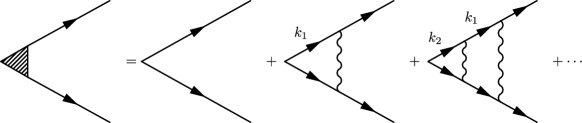
Figure 5: Perturbation expansion for the pairing vertex.

The renormalized vertex $\Phi$ depends on fermionic frequency $\omega_{m}$, fermionic momentum along the Fermi surface, $k_{\parallel}$, and on temperature. At high enough temperatures $\Phi(\omega_{m},k_{\parallel},T)$ weakly deviates from $\Phi_{0}$, but at $T_{c}$ the ratio $\Phi/\Phi_{0}$ should diverge for all frequencies and momenta. For definiteness, we set $k_{\parallel}$ to zero and $\omega_{m}$ to $\pi T$, i.e., consider $\Phi(\pi T,0,T)=\Phi(T)$. To simplify the formulas, we also set the ratio of Fermi velocities $\alpha=v_{y}/v_{x}$ to one.

Consider one-loop renormalization of $\Phi$ (the diagram with one wavy line in Fig. 5). After integration over momenta transverse to the Fermi surface (FS) we obtain, replacing the summation over $\omega_{m}$ by integration over $|\omega_{m}|>\pi T$,

$$\Phi(T)=\Phi_{0}\left(1+\pi(\omega_{0}\gamma)^{1/2}\int\frac{d\omega_{m}dk_{\parallel}}{4\pi^{2}}\frac{1}{|\omega_{m}+\Sigma(\omega_{m},k_{\parallel})|}\frac{1}{k^{2}_{\parallel}+\gamma|\omega_{m}|}\right)$$ (13)

where, we remind, $\Sigma(\omega_{m},k_{\|})={\rm sign}~{}\omega_{m}|\Sigma(\omega_{m},k_{\|})|$, and acs1 ; ms1

$$|\Sigma(\omega_{m},k_{\|})|=\sqrt{\omega_{0}}\left(\sqrt{|\omega|+k^{2}_{\parallel}/\gamma}-|k_{\parallel}|/{\sqrt{\gamma}}\right).$$ (14)

Rescaling $k_{\parallel}=(|\omega|\gamma)^{1/2}z$ we obtain

$$\Phi(T)=\Phi_{0}\left(1+\frac{\lambda}{2\pi}\int^{\infty}_{\pi T}\frac{d\omega_{m}}{\omega_{m}}\int dz\frac{\sqrt{z^{2}+1}+|z|}{z^{2}+1}\frac{1}{1+\left(\frac{\omega_{m}}{\omega_{0}}\right)^{1/2}(\sqrt{1+z^{2}}+|z|)}\right)$$ (15)

where $\lambda=2\alpha/(\alpha^{2}+1)=1$. One can easily make sure that the the integral in the r.h.s. of (15) contains $\log^{2}{\omega_{0}/T}$, which comes from large $z$, i.e., from $k^{2}_{\parallel}\gg|\omega_{m}|\gamma$ (Ref.ms1 ), and $\log{\omega_{0}/T}$, which comes from $z=O(1)$. The coupling constant $\lambda$ is one, so it is not obvious how to go beyond one-loop order. We choose a ”perturbative” path and artificially make $\lambda$ small by replacing $\lambda$ by ${\bar{\lambda}}=\varepsilon\lambda$ with $\varepsilon\ll 1$, such that ${\bar{\lambda}}\ll 1$. Then, obviously, ${\bar{\lambda}}\log^{2}{\omega_{0}/T}$ is more relevant than ${\bar{\lambda}}\log{\omega_{0}/T}$, i.e., to logarithmic accuracy ms1

$$\Phi(T)=\Phi_{0}\left(1+\frac{{\bar{\lambda}}}{2\pi}\log^{2}{\omega_{0}/T}\right)$$ (16)

We now check whether the series of ${\bar{\lambda}}\log^{2}{\omega_{0}/T}$ give rise to a pairing instability at $\log{\omega_{0}/T}\sim 1/\sqrt{{\bar{\lambda}}}$. Because $\log^{2}{\omega_{0}/T}$ comes from $k^{2}_{\parallel}\gg|\omega_{m}|\gamma$, we can expand the self-energy in $\gamma|\omega|/k^{2}_{\parallel}$, i.e., approximate $|\Sigma(\omega_{m},k_{\|})|$ in (14) by

$$|\Sigma(\omega_{m},k_{\|})|\approx 0.5\sqrt{\omega_{0}\gamma}\frac{\omega_{m}}{|k_{\parallel}|}$$ (17)

Using this self-energy, we obtain at two-loop order ($k_{\parallel,1}=k_{1},k_{\parallel,2}=k_{2}$)

$$\Phi(T) =\Phi_{0}\left(1+\frac{{\bar{\lambda}}}{2\pi}\log^{2}{\omega_{0}/T}+\frac{{\bar{\lambda}}^{2}}{4\pi^{2}}\int_{\sqrt{\gamma\pi T}}^{\sqrt{\gamma\Lambda}}\frac{2k_{1}dk_{1}}{k_{1}^{2}}\int_{\pi T}^{k_{1}^{2}/\gamma}\frac{d\omega_{1}}{\omega_{1}}\int_{\sqrt{\gamma\pi T}}^{\sqrt{\gamma\Lambda}}\frac{2k_{2}dk_{2}}{k_{2}^{2}+k_{1}^{2}}\int_{\pi T}^{k_{2}^{2}/\gamma}\frac{d\omega_{2}}{\omega_{2}}+O(\lambda^{3})\right)$$ (18)

Evaluating the integrals we find

$$\Phi(T) =\Phi_{0}\left(1+\frac{{\bar{\lambda}}}{2\pi}\log^{2}{\omega_{0}/T}+\frac{1}{2}\frac{{\bar{\lambda}}^{2}}{4\pi^{2}}\log^{4}{\omega_{0}/T}+...\right)$$ (19)

To understand what are the prefactors from higher-order terms, we note that $\log^{4}$ term comes from the region of internal momenta $k_{2}\gg k_{1}$, or, more specifically, the momentum $k_{1}$ in the cross-section which is farther from the vertex sets the lower cutoff of momentum integration over $k_{2}$ in the cross-section, which is closer to the vertex. This sheds light on the general pattern – we verified that at order $M$ the largest, $\log^{2M}{\omega_{0}/T}$ term comes from comes $k_{M}>k_{M-1}>...>k_{1}$, where $k_{M}$ is the momentum in the cross-section, which is the closest to the vertex. The same trend was earlier detected in the perturbation theory for the pairing vertex in 2D systems for which fermionic self-energy depends only on frequency acf1 . A simple exercise in combinatorics then yields, for the full series

$$\Phi(T) =\left(1+\frac{{\bar{\lambda}}}{2\pi}\log^{2}{\omega_{0}/T}+\frac{1}{2}\frac{{\bar{\lambda}}^{2}}{4\pi^{2}}\log^{4}{\omega_{0}/T}+\frac{1}{6}\frac{{\bar{\lambda}}^{3}}{8\pi^{3}}\log^{6}{\omega_{0}/T}+...\right)$$

$$=\Phi_{0}\sum^{\infty}_{M=0}\frac{{\bar{\lambda}}^{M}}{(2\pi)^{M}M!}\log^{2M}\frac{\omega_{0}}{T}=\Phi_{0}e^{({\bar{\lambda}}/2\pi)\log^{2}\omega_{0}/T}$$ (20)

We see that the calculation to $\log^{2}$ accuracy does not give rise to a pairing instability: the pairing susceptibility, $\Phi/\Phi_{0}$ increases with decreasing $T$, but does not diverge at any finite $T$.

III.1 A comparison with color superconductivity

The presence of $\log^{2}\omega_{0}/T$ in perturbation theory brings in the comparison with the problem of color superconductivity (CSC), where perturbative expansion also contains series of ${\bar{\lambda}}\log^{2}T$ terms. For that problem, however, previous works have demonstrated that the summation of $\log^{2}$ terms does lead to a pairing instability. It is therefore instructive to compare perturbation theory for CSC problem with our case and see where the two cases differ.

In CSC problem color1 ; joerg1 , as well as in condensed-matter problems of the pairing mediated by gapless collective excitations in three spatial dimensions moon1 , fermionic self-energy depends only on frequency (and is actually irrelevant to the pairing problem), and the extra logarithm, in addition to a Cooper one, appears because the effective interaction, integrated over momenta along the FS, has logarithmic dependence on frequency. Because the integration over momenta $k_{\parallel}$ can be done independently in any cross-section in Fig. 5, the pairing can be analyzed within the effective local model of fermions with dynamical interaction color1

$$\chi(\omega_{m})={\bar{\lambda}}\log{\frac{{\bar{\Lambda}}}{|\omega_{m}|}}$$ (21)

Substituting this form of the interaction (wavy line) into the one-loop diagram for $\Phi$, we obtain

$$\Phi(T)=\Phi_{0}\left(1+2{\bar{\lambda}}\int_{\pi T}^{{\bar{\lambda}}}\frac{d\omega}{\omega}\log{\frac{\Lambda}{|\omega|}}\right)=\Phi_{0}\left(1+{\bar{\lambda}}\log^{2}\frac{\Lambda}{\pi T}\right)$$ (22)

This is the same result as in our case. At two-loop order, however, the prefactor for ${\bar{\lambda}}^{2}\log^{4}{\Lambda/T}$ term is different from the one in our case. For CSC we have, at two-loop order

$$\Phi(T)= \Phi_{0}\left(1+{\bar{\lambda}}\log^{2}\frac{\Lambda}{\pi T}+{\bar{\lambda}}^{2}\int_{\pi T}^{\Lambda}\frac{2d\omega^{{}^{\prime}}}{\omega^{{}^{\prime}}}\log\frac{\Lambda}{|\omega^{{}^{\prime}}|}\int_{\pi T}^{\Lambda}\frac{2d\omega^{{}^{\prime\prime}}}{\omega^{{}^{\prime\prime}}}\log\frac{\Lambda}{|\omega^{{}^{\prime}}-\omega^{{}^{\prime\prime}}|}\right)$$ (23)

It is natural to divide the integration range over $\omega^{{}^{\prime\prime}}$ into two regimes, $\omega^{{}^{\prime\prime}}\gg\omega^{\prime}$ and $\omega^{{}^{\prime\prime}}\ll\omega^{\prime}$. It turns out that both regimes give contributions of order $\log^{4}{\Lambda/T}$. We have

$${\bar{\lambda}}^{2}\int_{\pi T}^{\Lambda}\frac{2d\omega^{\prime}}{\omega^{\prime}}\log\frac{\Lambda}{|\omega^{{}^{\prime}}|}\int_{\pi T}^{\Lambda}\frac{2d\omega^{\prime\prime}}{\omega^{\prime\prime}}\log\frac{\Lambda}{|\omega^{{}^{\prime}}-\omega^{{}^{\prime\prime}}|}$$

$$= {\bar{\lambda}}^{2}\int_{\pi T}^{\Lambda}\frac{2d\omega^{\prime}}{\omega^{\prime}}\log\frac{\Lambda}{{|\omega^{{}^{\prime}}|}}\left(\int_{\pi T}^{\omega^{\prime}}\frac{2d\omega^{\prime\prime}}{\omega^{\prime\prime}}\log\frac{\Lambda}{\omega^{\prime}}+\int_{\omega^{\prime}}^{\Lambda}\frac{2d\omega^{\prime\prime}}{\omega^{\prime\prime}}\log\frac{\Lambda}{\omega^{\prime\prime}}\right)$$

$$= {\bar{\lambda}}^{2}\left(2\int_{\pi T}^{\Lambda}\frac{2d\omega^{\prime}}{\omega^{\prime}}\log\frac{\Lambda}{{|\omega^{{}^{\prime}}|}}\log\frac{\omega^{\prime}}{\pi T}\log\frac{\Lambda}{\omega^{\prime}}+\int_{\pi T}^{\Lambda}\frac{2d\omega^{\prime}}{\omega^{\prime}}\log\frac{\Lambda}{|\omega^{\prime}|}\log^{2}\frac{\Lambda}{\omega^{\prime}}\right)$$

$$= {\bar{\lambda}}^{2}\left(\frac{1}{3}\log^{4}\frac{\Lambda}{\pi T}+\frac{1}{2}\log^{4}\frac{\Lambda}{\pi T}\right)$$

$$= \frac{5}{6}{\bar{\lambda}}^{2}\log^{4}\frac{\Lambda}{\pi T},$$ (24)

Combining one-loop and two-loop terms, we obtain

$$\Phi(T) =\Phi_{0}\left(1+{\bar{\lambda}}\log^{2}\frac{\Lambda}{\pi T}+\frac{5}{6}{\bar{\lambda}}^{2}\log^{4}\frac{\Lambda}{\pi T}\right)$$ (25)

which is different from the two-loop result in our case, Eq. (19). The difference comes about because for CSC there is no requirement that highest power of the logarithm comes from particular hierarchy of running frequencies – at two loop order, there is $\log^{4}$ contribution from the range where the highest frequency in the cross-section next to the vertex, and from the range when the highest frequency is in the cross-section farthest from the vertex.

The series of ${\bar{\lambda}}\log^{2}$ terms for CSC problem have been summed up in Ref. joerg1 , an the result is

$$\Phi(\omega=\pi T) =\Phi_{0}\left(1+{\bar{\lambda}}\log^{2}\frac{\Lambda}{\pi T}+\frac{5}{6}{\bar{\lambda}}^{2}\log^{4}\frac{\Lambda}{\pi T}+O({\bar{\lambda}}^{3})\right)$$

$$=\frac{\Phi_{0}}{\cos[(2{\bar{\lambda}}\log^{2}\Lambda/\pi T)^{1/2}]}$$ (26)

IV Linearized gap equation

IV.1 Interplay between characteristic momenta and frequency

We start with the Eq (5) in the main text. We first discuss the case where $\alpha=1$. In this case ${\bar{\lambda}}=2\varepsilon\alpha/(1+\alpha^{2})=\varepsilon$. Treating $\varepsilon$ again as a small parameter, we have

$$\Phi(\omega_{m},k_{\parallel})=\varepsilon\pi\left(\omega_{0}\gamma\right)^{1/2}T\sum_{m^{\prime}}\int\frac{dk^{\prime}_{\parallel}}{2\pi}\frac{\Phi(\omega_{m^{\prime}},k^{{}^{\prime}}_{\parallel})}{|\omega_{m^{\prime}}+\Sigma(\omega_{m^{\prime}},k^{{}^{\prime}}_{\parallel})|}\times\frac{1}{k^{2}_{\parallel}+k^{{}^{\prime}2}_{\parallel}+\gamma|\omega_{m}-\omega_{m^{{}^{\prime}}}|}$$ (27)

where the self-energy $\Sigma$ is given by (14). The dependence on system parameters $\omega_{0}$ and $\gamma$ can be eliminated if we measure $\omega$ and $T$ in units of $\omega_{0}$, and measure $k_{\parallel}$ in units of $(\omega_{0}\gamma)^{1/2}$. Introducing ${\bar{\omega}}=\omega/\omega_{0}$, ${{\bar{T}}}=\pi T/\omega_{0}$, and ${\bar{k}}_{\parallel}=k_{\parallel}/(\omega_{0}\gamma)^{1/2}$, we re-write (27) as

$$\Phi({\bar{\omega}}_{m},{\bar{k}}_{\parallel})=\varepsilon{{\bar{T}}}\sum_{m^{\prime}}\int\frac{d{\bar{k}}^{\prime}_{\parallel}}{2\pi}\frac{\Phi({\bar{\omega}}_{m^{\prime}},{\bar{k}}^{{}^{\prime}}_{\parallel})}{|{\bar{\omega}}_{m^{\prime}}+{\bar{\Sigma}}({\bar{\omega}}_{m^{\prime}},{\bar{k}}^{{}^{\prime}}_{\parallel})|}\times\frac{1}{{\bar{k}}^{2}_{\parallel}+{\bar{k}}^{{}^{\prime}2}_{\parallel}+|{\bar{\omega}}_{m}-{\bar{\omega}}_{m^{{}^{\prime}}}|},$$ (28)

where

$${\bar{\Sigma}}({\bar{\omega}}_{m},{\bar{k}}_{\|})=\left(\sqrt{|{\bar{\omega}}|+{\bar{k}}^{2}_{\parallel}}-|{\bar{k}}_{\parallel}|\right)$$ (29)

The question we address is whether $T_{c}$ is non-zero already at arbitrary small $\varepsilon$, or it only emerges when $\varepsilon$ exceeds a certain threshold.

Because $\varepsilon$ is treated as small parameter, ${{\bar{T}}}_{c}$ is expected to be small, and to get the pairing we need to explore logarithmical behavior which comes from frequency scale larger than $T_{c}$. Accordingly, we replace ${{\bar{T}}}\sum_{m^{\prime}}$ by $(1/2)\int d\bar{\omega}_{m^{\prime}}$ and set $\pm\bar{T}$ as the lower limits of the integration over positive and negative $\omega_{m^{\prime}}$, respectively. We then have, instead of (28)

$$\Phi({\bar{\omega}}_{m},{\bar{k}}_{\parallel})=\frac{\varepsilon}{2}\int d{\bar{\omega}}_{m^{\prime}}\int\frac{d{\bar{k}}^{\prime}_{\parallel}}{2\pi}\frac{\Phi({\bar{\omega}}_{m^{\prime}},{\bar{k}}^{{}^{\prime}}_{\parallel})}{|{\bar{\omega}}_{m^{\prime}}+{\bar{\Sigma}}({\bar{\omega}}_{m^{\prime}},{\bar{k}}^{{}^{\prime}}_{\parallel})|}\times\frac{1}{{\bar{k}}^{2}_{\parallel}+{\bar{k}}^{{}^{\prime}2}_{\parallel}+|{\bar{\omega}}_{m}-{\bar{\omega}}_{m^{{}^{\prime}}}|},$$ (30)

In general, $\Phi({\bar{\omega}}_{m},{\bar{k}}_{\parallel})$ is a function of both arguments, but in proper limits the dependence on one of the arguments is stronger than on the other. In the main text we consider the limits ${\bar{k}}^{2}_{\parallel}\gg{\bar{\omega}}_{m}$ and ${\bar{k}}^{2}_{\parallel}\ll{\bar{\omega}}_{m}$. In the first case, the momentum dependence is stronger than frequency dependence, and $\Phi({\bar{\omega}}_{m},{\bar{k}}_{\parallel})$ can be approximated by $\Phi({\bar{k}}_{\parallel})$. The fermionic self-energy at ${\bar{k}}^{2}_{\parallel}\gg{\bar{\omega}}_{m}$ behaves as

$${\bar{\Sigma}}({\bar{\omega}}_{m},{\bar{k}}_{\|})\approx\frac{|{\bar{\omega}}_{m}|}{2|{\bar{k}}_{\parallel}|}$$ (31)

Substituting this form into (30) we obtain

$$\Phi({\bar{k}}_{\|})=\frac{2\varepsilon}{\pi}\int\frac{{\bar{k}}^{\prime}_{\|}d{\bar{k}}^{\prime}_{\|}}{{\bar{k}}_{\|}^{2}+{\bar{k}}_{\|}^{{}^{\prime}2}}\frac{1}{2{\bar{k}}^{\prime}_{\|}+1}\Phi(k^{\prime}_{\|})\int_{{{\bar{T}}}}^{{\bar{k}}_{\|}^{2}}\frac{d{\bar{\omega}}^{{}^{\prime}}_{m}}{{\bar{\omega}}^{{}^{\prime}}_{m}}.$$ (32)

Integrating explicitly over $\omega_{m}$ and introducing new variable $x={\bar{k}}_{\|}^{{}^{\prime}2}/{{\bar{T}}}$ , we obtain Eq 6 in the main text.

$$\Phi(y)=\frac{\varepsilon}{\pi}\int_{1}\frac{dx}{x+y}\frac{\log{x}}{2\sqrt{x{{\bar{T}}}}+1}\Phi(x),$$ (33)

In the opposite limit, ${\bar{k}}^{2}_{\parallel}\ll{\bar{\omega}}$, the momentum dependence of the self-energy is small, and ${\bar{\Sigma}}$ can be approximated by its value at the hot spot, i.e., ${\bar{\Sigma}}\approx\sqrt{|{\bar{\omega}}_{m}|}$. This limit can only be justified at small or large ratio of $v_{y}/v_{x}$ because otherwise substituting this ${\bar{\Sigma}}$ into (30) we obtain that typical internal ${\bar{k}}^{{}^{\prime}2}_{\parallel}$ are of order ${\bar{\omega}}^{{}^{\prime}}$. Nevertheless, if we assume that the momentum dependence of the fermionic self-energy can be neglected, at least for order-of-magnitude estimates, we obtain that $\Phi({\bar{\omega}}_{m},{\bar{k}}_{\parallel})$ can be approximated by $\Phi({\bar{\omega}}_{m})$, and the gap equation becomes acs1 ; acf1

$$\Phi({\bar{\omega}}_{m})=\frac{\pi\varepsilon{{\bar{T}}}}{2}\sum_{m^{\prime}}\frac{\Phi({\bar{\omega}}_{m^{\prime}})}{\sqrt{|{\bar{\omega}}_{m^{\prime}}|}\sqrt{|{\bar{\omega}}_{m}-{\bar{\omega}}_{m^{\prime}}|}(1+\sqrt{|{\bar{\omega}}_{m^{\prime}}|})}.$$ (34)

This is Eq. (9) in the main text.

IV.2 Solution of the Eq. 33

We first replace the soft cutoff imposed by $\left(2\sqrt{x{\bar{T}}}+1\right)^{-1}$ with a hard cutoff,

$$\Phi(y)=\frac{\varepsilon}{\pi}\int_{1}^{1/{{\bar{T}}}}\frac{dx}{x+y}\log x~{}\Phi(x)$$ (35)

The integration over $x\gg y$ gives rise to $\log^{2}$ terms in the perturbation theory, which, as we know from the analysis in the previous section, do not give rise to the pairing instability. We therefore focus on the range $x\sim y$. The contribution from this range gives rise to a single logarithm ($\log 1/{{\bar{T}}}$) if we momentary assume that $\Phi(x)$ is a constant. Like we did before, we treat $\varepsilon$ as a small parameter and check whether Eq. (35) has a solution at a finite ${{\bar{T}}}$.

For small $\varepsilon$, ${\bar{T}}$ is expected to be also small, i.e., the upper limit of the integration in (35) is a large number. We first consider $y$ and $x\sim y$ in the range $1\ll y,x\ll 1/{\bar{T}}$, and search for the solution of (35) in the form $\Phi(x)=\exp[-f(p(x))]$, where $p(x)=\varepsilon\log{x}$. Plugging this function back into the equation and introducing a new variable $z=x/y$, we obtain,

$$e^{-f(\varepsilon\log y)}=\frac{\varepsilon}{\pi}\log y\int_{\frac{1}{y}}^{\infty}\frac{dz}{z+1}\left(1+\frac{\log z}{\log y}\right)e^{-f(\varepsilon(\log y+\log z))}$$ (36)

We assume and then verify that typical $z$ are of order one, i.e., $\log z\ll\log y$. Taylor expanding in $\log z/\log y$ we obtain

$$1= \frac{\varepsilon}{\pi}\log y~{}\int_{0}^{\infty}\frac{dz}{z+1}\frac{1}{z^{Q(\varepsilon\log y)}}$$

$$= \varepsilon\log y~{}\frac{1}{\sin(\pi Q(\varepsilon\log y))}.$$ (37)

where we introduced

$$Q(p)\equiv\frac{df(p)}{dp}.$$ (38)

Solving (37) we obtain

$$Q(\varepsilon\log y)=\frac{1}{\pi}\arcsin(\varepsilon\log y).$$ (39)

Integrating over $\log y$, we have

$$f(p)=\frac{1}{\pi\varepsilon}\left[p\arcsin\left(p\right)+\sqrt{1-p^{2}}-1\right],$$ (40)

which is Eq 7 of the main text.

Lastly we consider the boundary condition at $y=y_{0}=1/{{\bar{T}}}$. For such $y$, the upper limit is 1. Substituting formally the trial solution $\Phi(x)=\exp[-f(p(x))]$ into the r.h.s. of (35) we obtain

$$1=\frac{\varepsilon}{\pi}\log y_{0}~{}\int_{0}^{1}\frac{dz}{z+1}\frac{1}{z^{Q(2\pi\varepsilon\log y_{0})}}$$ (41)

One can easily make sure that to satisfy this equation, $Q(\varepsilon\log y_{0})$ must be larger than if we take our result, Eq. (39), and set $y=y_{0}$ there. At vanishingly small ${\bar{T}}$, the presence of the upper limit of the integration over $x$ in (35) becomes relevant only for $y$ infinitesimally close to $y_{0}$ (for smaller $y$, the upper limit can be safely set to infinity). This implies that at ${\bar{T}}\to 0$, $Q(p)$ undergoes a finite jump at $y=y_{0}$, hence at the actual $T=T_{c}$

$$\frac{dQ(p)}{dp}\bigg{|}_{p=\varepsilon\log{1/\bar{T}}_{c}}=\infty.$$ (42)

This last equation is satisfied if $\varepsilon\log 1/{\bar{T}_{c}}=1$ Restoring the parameters, we then obtain Eq 8 in the main text. For this $T_{c}$, the jump in $Q$ at the boundary is between $Q=0.5$ (Eq. (39) at $y=y_{0}=1/{\bar{T}}_{c}$) and $Q=0.73$, which is the solution of (41) at $T_{c}$.

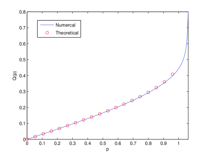
Figure 6: Numerical solution of $Q(p)$ and its comparison with theory. We set $\varepsilon=1.5\times 10^{-2}$.

In Fig. 6 we plot $Q(p)$ obtained from the numerical solution of Eq. (35) and compare it with the (approximate) analytical solution presented in this section. We see that the agreement is quite good.

IV.3 Gap equation for $\alpha\neq 1$

The reasoning we used in the previous section can be extended to the case of a general $\alpha$.

We follow the same procedure leading to Eq. 35, only this time we keep explicit $\alpha$ dependence along the way. We introduce new, $\alpha$-dependent variable $x$ as $x=2\alpha/(\alpha^{2}+1)~{}\bar{k}_{\|}^{{}^{\prime}2}/\bar{T}$ and obtain an $\alpha$ dependent version of Eq. 35,

$$\Phi(y)=\frac{\bar{\lambda}}{\pi}\int_{1}^{1/\bar{T}}\frac{(x+y)~{}dx}{(x+y)^{2}-4\mu^{2}xy}\log x~{}\Phi(x),$$ (43)

where $\mu=(1-\alpha^{2})/(1+\alpha^{2})$ and, we remind, ${\bar{\lambda}}=2\varepsilon\alpha/(1+\alpha^{2})$. We again assume and then verify that the major contribution to the r.h.s. of (43) comes from $x\sim y$, i.e., $z\sim 1$, and, as before, introduce $p=\varepsilon\log y$ and the same $Q(p)$ as in (38). We then obtain for $1\ll y,x\ll 1/\bar{T}$,

$$1=\frac{\varepsilon\lambda}{\pi}\log y\int_{0}^{\infty}\frac{(z+1)~{}dz}{(z+1)^{2}-4\mu^{2}z}\frac{1}{z^{Q(\varepsilon\log y)}}.$$ (44)

or

$$p=\frac{\pi}{\lambda I(Q(p),\mu)},$$ (45)

where

$$I(Q,\mu)=\int_{0}^{\infty}\frac{(z+1)~{}dz}{(z+1)^{2}-4\mu^{2}z}\frac{1}{z^{Q(\varepsilon\log y)}}.$$ (46)

We know from previous section that the upper boundary for $x\sim y$ is $x,y\sim 1/{\bar{T}}_{c}$, or $p=\varepsilon\log{1/{\bar{T}}_{c}}$, and that at the upper boundary $\frac{dQ(p)}{dp}\big{|}_{p=\varepsilon\log{1/\bar{T}}_{c}}=\infty$, or, $\frac{dp}{dQ}\big{|}_{p=\varepsilon\log{1/\bar{T}}_{c}}=0$. Combining this with Eq. 45, we obtain

$$\frac{dp}{dQ}\bigg{|}_{p=\varepsilon\log{1/\bar{T}}_{c}}\propto\frac{dI}{dQ}\bigg{|}_{p=\varepsilon\log{1/\bar{T}}_{c}}{=}0.$$ (47)

Hence, at $y=\bar{T}_{c}$, ${dI}/{dQ}=0$. It is easy to see from (46) that $I(Q)=I(1-Q)$, therefore the boundary condition sets $Q=1/2$. Plugging $p=\varepsilon\log{1/\bar{T}}_{c}$ and $Q=1/2$ back to Eq. 45, we obtain

$$\varepsilon\log{1/\bar{T}}_{c}=\frac{\pi}{\lambda I(Q=1/2,\mu)}.$$ (48)

The integral for $I(Q=1/2,\mu)$ can be easily evaluated, and we obtain

$$I(Q=1/2,\mu) =\int_{0}^{\infty}\frac{1+z}{(1+z)^{2}-4\mu^{2}z}~{}\frac{dz}{z^{1/2}}$$

$$=\frac{\pi}{\sqrt{1-\mu^{2}}}$$

$$=\frac{\pi}{\lambda}.$$ (49)

where in the last step we used the fact that $\mu^{2}+\lambda^{2}=1$. Substituting this finally into (48) we obtain $\varepsilon\log 1/\bar{T}_{c}=1$, i.e., $T_{c}\sim{\omega_{0}}e^{-1/\varepsilon}$, independent on $\alpha$.

We emphasize that independence of $T_{c}$ on $\alpha$ could not be seen from naive perturbation analysis, since back there the prefactor ${\bar{\lambda}}$ for the $\log^{2}$ term was $\alpha$ dependent. For verification, we solved Eq 43 numerically for various $\alpha$ and indeed find that $T_{c}$ does not change when $\alpha$ changes.

IV.4 The case of strong nesting

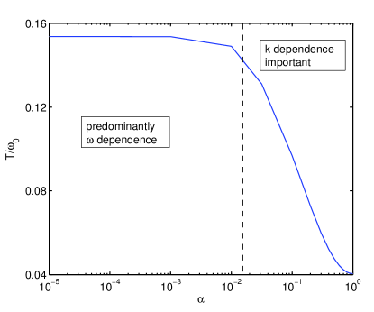
Figure 7: Numerical solution of Eq. (27) for various $\alpha=v_{y}/v_{x}$ (the Fermi velocities at hot spots separated by $(\pi,\pi)$ are ${\bf v}_{F,1}=(v_{x},v_{y})$ and ${\bf v}_{F,2}=(-v_{x},v_{y})$. We set ${\bar{g}}a/v_{F}\approx 0.032$. For $\alpha=O(1)$ the momentum dependence of the fermionic self-energy is relevant, and $T_{c}\approx 0.04\omega_{0}$. At smaller $\alpha$, when $\alpha<({\bar{g}}/(v_{F}/a))^{2/3}$ (to the left of vertical dashed line), frequency dependence of the self-energy prevails, the pairing comes exclusively from fermions with non-FL self-energy, and $T_{c}\approx 0.17\omega_{0}$, up to corrections of order $({\bar{g}}a/v_{F})^{1/2}$. In our case, these corrections reduce this number from $0.17$ to $0.15$.

At strong nesting, when velocities at ${\bf k}_{F}$ and ${\bf k}_{F}+{\bf Q}$ are nearly antiparallel, $\alpha\ll 1$ and $\gamma\propto 1/\alpha$ is large. In this situation, the pairing eventually become determined by fermions whose self-energy has a non-FL form. This happens when $(\gamma\omega_{0})^{1/2}$ becomes larger than maximal possible $\alpha|k_{\parallel}|$ along a Fermi arc, which is of order $1/a$, i.e., when $v_{F}/a\gg{\bar{g}}>\alpha v_{F}/a$. In this situation, the momentum dependence of $\Sigma(\omega_{m},k_{\parallel})$ becomes irrelevant at $\omega_{m}\sim\omega_{0}$, $\Phi(\omega_{m},k_{\parallel})$ becomes predominantly frequency-dependent, and $T_{c}$ recovers the value $0.17\omega_{0}$, which is $T_{c}$ for momentum-independent self-energy. We verified numerically that this is indeed the case. We plot $T_{c}$ vs $\alpha$ in Fig. 7. At $\alpha=O(1)$, $T_{c}\approx 0.04\omega_{0}$, and at small enough $\alpha$, $T_{c}$ approaches $0.17\omega_{0}$. We caution, however, that the limit $\alpha\ll 1$ has to be taken with care as nesting may generate additional singularities at higher-loop orders.

References

- (1)
- (2) S. Sachdev and B. Keimer, Physics Today, 64, 29, (2011).
- (3) K. Hashimoto et al., Science 336, 1554 (2012).
- (4) A. Chubukov, D. Pines and J. Schmalian A Spin Fluctuation Model for D-wave Superconductivity in ‘The Physics of Conventional and Unconventional Superconductors’ edited by K.H. Bennemann and J.B. Ketterson (Springer-Verlag), 2002.
- (5) H. v. Löhneysen, A. Rosch, M. Vojta, and P. Wölfle, Rev. Mod. Phys. 79, 1015 (2007).
- (6) E. Fradkin, S. A. Kivelson, M. J. Lawler, J. P. Eisenstein, A. P. Mackenzie, Annual Reviews of Condensed Matter Physics 1, 153 (2010).
- (7) P. A. Lee, Phys. Rev. Lett. 63, 680 (1989); J. Polchinski, Nucl. Phys. B 422, 617 (1994); Y.-B. Kim, A. Furusaki, X.-G. Wen, and P. A. Lee, Phys. Rev. B 50, 17917 (1994); C. Nayak and F. Wilczek, Nucl. Phys. B 417, 359 (1994); 430, 534 (1994); B. L. Altshuler, L. B. Ioffe, and A. J. Millis, Phys. Rev. B 50, 14048 (1994); 52, 5563 (1995); S. Chakravarty, R. E. Norton, and O. F. Syjuasen, Phys. Rev. Lett. 74, 1423 (1995); C.J. Halboth and W. Metzner, Phys. Rev. Lett. 85, 5162 (2000); J. Quintanilla and A. J. Schofield, Phys. Rev. B 74, 115126 (2006); J. Rech, C. Pépin, and A. V. Chubukov, Phys. Rev. B 74, 195126 (2006); T. Senthil, Phys. Rev. B 78, 035103 (2008); M. Zacharias, P. Wölfle, and M. Garst, Phys. Rev. B80, 165116 (2009); D.L. Maslov and A.V. Chubukov, Phys. Rev. B81, 045110 (2010). M.A. Metlitski and S. Sachdev, Phys. Rev. B 82, 075127 (2010); D. F. Mross, J. McGreevy, H. Liu, and T. Senthil, Phys. Rev. B 82, 045121 (2010).
- (8) A. J. Millis, S. Sachdev, and C. M. Varma, Phys. Rev. B 37, 4975 (1988).
- (9) Ar. Abanov, A. V. Chubukov, and A.M. Finkelstein, Europhys. Lett. 54, 488 (2001).
- (10) A. Abanov, A. V. Chubukov, and J. Schmalian, Adv. Phys., 52, 119 (2003).
- (11) E.G. Moon and A.V. Chubukov, J. Low Temp. Phys., 161, 263-281 (2010).
- (12) E. G. Moon, and S. Sachdev, Phys. Rev. B 80, 035117 (2009).
- (13) N. E. Bonesteel, I. A. McDonald, and C. Nayak, Phys. Rev. Lett. 77, 3009 (1996).
- (14) Ar. Abanov, B. Altshuler, A. Chubukov, and E. Yuzbashyan, unpublished.
- (15) D. V. Khveshchenko and W. F. Shively, Phys. Rev. B 73, 115104 (2006); A. V. Chubukov and A. M. Tsvelik, Phys. Rev. B 76, 100509 (2007).
- (16) A. Chubukov, and J. Schmalian, Phys. Rev. B. 72, 174520 (2005).
- (17) D. T. Son, Phys. Rev. D. 59, 094019 (1999).
- (18) M.A. Metlitski and S. Sachdev, Phys. Rev. B 82, 075128 (2010).
- (19) A.J. Millis, Phys. Rev. B 45, 13047 (1992).
- (20) S.-S. Lee, Phys. Rev. B 80, 165102 (2009).
- (21) S. A. Hartnoll, D. M. Hofman, M. A. Metlitski, and S. Sachdev Physical Review B 84, 125115 (2011); E. Berg, M. A. Metlitski, and S. Sachdev, arXiv:1206.0742.
- (22) Ar. Abanov, A.V. Chubukov, and M. Norman, Phys. Rev. B 78, 220507 (2008).
- (23) M. Salmhofer et al, Prog. Theor. .Phys. 112, 943 (2004); K. Le Hur and T. M. Rice, Annals of Physics 324 (2009) 1452; R. Nandkishore, L. Levitov, and A. V. Chubukov, Nature Physics 8 158 (2012).
- (24) A. V. Chubukov, D. Efremov, and I. Eremin, Phys. Rev. B 78, 134512 (2008); V. Cvetkovic and Z. Tesanovic, Phys. Rev. B 80, 024512(2009); Fa Wang, H. Zhai, Y. Ran, A. Vishwanath, and D-H Lee, Phys. Rev. Lett. 102, 047005 (2009); R. Thomale, C. Platt, J-P. Hu, C. Honerkamp, and B. A. Bernevig, Phys. Rev. B 80, 180505 (2009).
- (25) A. Sedeki, D. Bergeron, and C. Bourbonnais, Phys. Rev. B 85, 165129 (2012).
- (26) Hui Zhai, Fa Wang, and Dung-Hai Lee, Phys. Rev. B 80, 064517 (2009).
- (27) D. Scalapino, Phys. Rep., 250, 329 (1995).
- (28) M.A Metlitski et al, unpublished.
- (29) P. Monthoux and D. J. Scalapino, Phys. Rev. Lett. 72, 1874 (1994); T. Dahm and L. Tewordt, Phys. Rev. B 52, 1297 (1995); D. Manske, I. Eremin and K. H. Bennemann, Phys. Rev. B 67, 134520 (2003); St. Lenck, J. P. Carbotte and R. C. Dynes, Phys. Rev. B 50, 10149 (1994); B. Kyung, J.-S. Landry, A.-M. S. Tremblay, Phys. Rev. B 68, 174502 (2003); T. Maier et al., Phys. Rev. Lett. 95, 237001 (2005); K. Haule and G. Kotliar, Phys. Rev. B 76, 104509 (2007); S. S. Kancharla et al., Phys. Rev. B 77, 184516 (2008); D. Senechal and A-M. S. Tremblay, Phys. Rev. Lett. 92, 126401 (2004).
- (30) Ar. Abanov and A.V. Chubukov, Phys. Rev. Lett., 93, 255702 (2004).

References

- (1) A. Abanov, A. V. Chubukov, and J. Schmalian, Adv. Phys., 52, 119 (2003).
- (2) M.A. Metlitski and S. Sachdev, Phys. Rev. B 82, 075128 (2010).
- (3) Ar. Abanov, A. V. Chubukov, and A.M. Finkelstein, Europhys. Lett. 54, 488 (2001).
- (4) D. T. Son, Phys. Rev. D. 59, 094019 (1999).
- (5) A. Chubukov, and J. Schmalian, Phys. Rev. B. 72, 174520 (2005).
- (6) E.G. Moon and A.V. Chubukov, J. Low Temp. Phys., 161, 263-281 (2010).
- (7) S. A. Hartnoll, D. M. Hofman, M. A. Metlitski, and S. Sachdev Physical Review B 84, 125115 (2011)
- (8) T. A. Maier, M. S. Jarrell, and D. J. Scalapino Phys. Rev. Lett. 96, 047005 (2006).
- (9) M. Salmhofer et al, Prog. Theor. .Phys. 112, 943 (2004); K. Le Hur and T. M. Rice, Annals of Physics 324 (2009) 1452; R. Nandkishore, L. Levitov, and A. V. Chubukov, Nature Physics 8 158 (2012).
- (10) A. V. Chubukov, D. Efremov, and I. Eremin, Phys. Rev. B 78, 134512 (2008); V. Cvetkovic and Z. Tesanovic, Phys. Rev. B 80, 024512(2009); Fa Wang, H. Zhai, Y. Ran, A. Vishwanath, and D-H Lee, Phys. Rev. Lett. 102, 047005 (2009); R. Thomale, C. Platt, J-P. Hu, C. Honerkamp, and B. A. Bernevig, Phys. Rev. B 80, 180505 (2009).
- (11) A. Sedeki, D. Bergeron, and C. Bourbonnais, Phys. Rev. B 85, 165129 (2012).
- (12) Hui Zhai, Fa Wang, and Dung-Hai Lee, Phys. Rev. B 80, 064517 (2009).
- (13) D.L. Maslov and A.V. Chubukov, Phys. Rev. B 81, 045110 (2010).