Exchange interactions and local moment fluctuation corrections in ferromagnets at finite temperatures based on non-collinear density-functional calculations

Abstract

We explore the derivation of interatomic exchange interactions in ferromagnets within density-functional theory (DFT) and the mapping of DFT results onto a spin Hamiltonian. We delve into the problem of systems comprising atoms with strong spontaneous moments together with atoms with weak induced moments. All moments are considered as degrees of freedom, with the strong moments thermally fluctuating only in angle and the weak moments thermally fluctuating in angle and magnitude. We argue that a quadratic dependence of the energy on the weak local moments magnitude, which is a good approximation in many cases, allows for an elimination of the weak-moment degrees of freedom from the thermodynamic expressions in favor of a renormalization of the Heisenberg interactions among the strong moments. We show that the renormalization is valid at all temperatures accounting for the thermal fluctuations and resulting in temperature-independent renormalized interactions. These are shown to be the ones directly derived from total-energy DFT calculations by constraining the strong-moment directions, as is done e.g. in spin-spiral methods. We furthermore prove that within this framework the thermodynamics of the weak-moment subsystem, and in particular all correlation functions, can be derived as polynomials of the correlation functions of the strong-moment subsystem with coefficients that depend on the spin susceptibility and that can be calculated within DFT. These conclusions are rigorous under certain physical assumptions on the measure in the magnetic phase space. We implement the scheme in the full-potential linearized augmented plane wave (FLAPW) method using the concept of spin-spiral states, considering applicable symmetry relations and the use of the magnetic force theorem. Our analytical results are corroborated by numerical calculations employing DFT and a Monte Carlo method.

I Introduction

In recent years there has been increasing activity in the prediction of high-temperature magnetic properties of solids, especially regarding critical magnetic transition temperatures. The theoretical approach is founded in many cases on two assumptions: (i) that the magnetic excitations of a system can be phenomenologically described within a classical or quantum Heisenberg model, and (ii) that the exchange parameters entering the model (i.e., the excitation energies) can be microscopically derived from total energy results of e.g. density-functional theory calculations. This “magnetic multi-scale modelling” has proven succesful in many cases, including itinerant elemental ferromagnets such as Fe and Co,MacLaren99 ; Pajda01 ; Shallcross05 ; Lezaic07 localized-moment systems such as Gd,Turek03 ; Khmelevskyi07 magnetic alloys as NiMnSb or Co₂MnSi,Sasioglu05 or diluted magnetic semiconductors as (Ga,Mn)As.Sato04 ; Bergqvist04 In these systems, the estimated Curie temperatures $T_{\mathrm{C}}$ are within 10-15% of the experimental values, showing that the approach is reliable for practical purposes.

The derivation of magnetic excitation energies from density-functional calculations requires additional assumptions, since density-functional theory is, in principle, valid only for the description of the ground state of many-electron systems. Mainly, one relies on an adiabatic hypothesis, which conjectures that the slow motion of low-energy magnetic excitations can be decoupled from the fast motion of intersite electron hopping, so that the local electronic structure has time to relax under the constraint that a magnon traverses the system. Then the magnons are regarded as practically static or “frozen” objects, and constrained density functional theoryDederichs84 is employed. This adiabatic approximation, together with the realization that the local moments persist until above the Curie temperature, constitutes a paradigm which has proven fruitful. Quite a few theories and methods have been based on it, aimed at the calculation of thermodynamic quantities, including $T_{\mathrm{C}}$, by harvesting the model parameters from first principles calculations and working out the thermodynamics within Monte Carlo methods or other suitable approaches.

Among the first to discuss the adiabatic approximation in connection to DFT calculations were Gyorffy and co-workers in the development of a mean-field theory of magnetic fluctuations,Gyorffy85 even though the concept was applied earlier on the level of solutions to many-body model Hamiltonians (see e.g. Small and HeineSmall84 ). Later Antropov et al.Antropov96 and Halilov et al.Halilov98 derived equations for adiabatic ab-initio spin dynamics. Further elaboration came from Niu and collaboratorsNiu99 and Gebauer and Baroni,Gebauer00 who showed that the Berry curvature enters the adiabatic dynamics equations; they also demonstrated mathematically how the Born-Oppenheimer method can be generalized for adiabatic spin dynamics without the requirement that there should be a large mass difference defining the time-scale difference.

Based on the adiabatic approximation, a proper parametrization of the excitation spectrum is called for. In many, but not all, ferromagnetic systems the magnitude of the local atomic moments is relatively robust under modest rotations, so that mainly the pair exchange constants entering a Heisenberg model are required. From the point of view of methodology, two approaches are commonly used for the determination of the pair exchange constants. The first is based on multiple-scattering theory and Green function methods, frequently in the approximation of infinitesimal rotations.Liechtenstein87 It is widely used in methods where the Green function is available.FrotaPessoa00 ; Pajda01 ; Sato04 ; MacLaren99 ; Katsnelson00 ; Rusz06 ; Ruban07 ; Polesya10 ; Szunyogh11 ; Dias11 A variant of this approach is the use of the disorder-local-moment (DLM) reference stateGyorffy85 as an approximation to the magnetic disorder at the Curie temperature, from which one obtains exchange parametersOguchi83 ; Oguchi83b in a manner analogous to the method of infinitesimal rotations.Liechtenstein87 Higher-order interactions (e.g. the biquadratic, 4-th order, or anisotropic exchange) can be also obtained in a systematic way either from the ferromagnetic ground stateUdvardi03 ; Ebert09 or from the DLM state.Szunyogh11

The second approach, which we follow in this work, is based on reciprocal-space calculation of spin-wave excitation energies by constraining the system to spin spirals of given wavevectors $\bm{q}$. This requires non-collinear calculations, restricted to the primitive chemical unit cell (in the absence of spin-orbit coupling) by virtue of a generalized Bloch theorem.Sandratskii86 A subsequent integration in $\bm{q}$-space (in form of a back-Fourier transformation) yields the pair exchange constants. Although the force theoremAndersen is in principle not necessary here, practically it is often used in order to avoid the numerical load of a self-consistent calculation for each vector $\bm{q}$. This second approach is well-suited for electronic structure methods which are based on Hamiltonian diagonalization rather than Green functions, and has been developed, for example, for the augmented spherical wave (ASW) methodSandratskii02 ; Kubler06 or the LMTO method.Halilov98 Concerning the second approach, we should also mention that a proper energy fit to a large number of constrained-moment-directions has been used to extract model parameters, inspired by alloy-theory methods, for example by applying the Connolly-Williams theoryConnolly83 to fit a number of antiferromagnetic statesPeng91 or in a more refined way by applying a systematic spin-cluster expansion including higher-order interactionsDrautz04 ; Singer11 for a fit to non-collinear states.

The results of the two approaches (infinitesimal rotations and spin-wave spectra) on the values of exchange interactions agree well, at least as long as the density-functional calculations are done within the same electronic structure method.FrotaPessoa00 There is also good agreement in the spin-wave spectra of the two approaches if these are calculated in the first approach from a Fourier-transformation of the real space coupling parameters, as long as a sufficiently large number of atomic shells is taken in the Fourier series.Rusz06

The present paper contains two major parts. In the first part, Sections II and III, we start by presenting the formalism for the calculation of pair exchange constants which we have implemented in the full-potential augmented linearized plane wave (FLAPW) method.Wimmer81 ; FLEUR The approach of spin spirals and inverse Fourier transformationsHalilov98 is used to arrive at formulae for the pair exchange constants in the case of one or more magnetic atoms per unit cell. Symmetry relations are derived that reduce the selection of spin-spirals to the irreducible part of the Brillouin zone. Then, we focus on accuracy tests concerning the use of the force theorem at finite rotations; we also address the problem of subtracting the contribution of the magnetization in the interstitial. As a test, we calculate the Curie temperature of certain compounds by a Monte Carlo method. In the second part, Section IV, we discuss a way to parametrize the energetic contribution of longitudinal changes in the atomic spin moment so as to include them in a Monte Carlo method in the case that we are faced with a compound containing strong-moment and induced-moment sublattices. We obtain a scheme for the study of temperature-dependent magnetic properties and derive equations that allow a simplification of the computational method and a reduction of the computational cost under certain frequently-met physical conditions; importantly, we show the hitherto unnoticed result that the fluctuating weak-moment degrees of freedom can be analytically eliminated in favour of renormalized, temperature-independent strong-moment interactions, and that the thermodynamics of the full system (strong plus weak moments with bare interactions) can be derived from the thermodynamics of the strong-moment system only with renormalized interactions (a general derivation is given in the Appendix). A numerical demonstration of this rigorous result is presented in the case of the half-Heusler alloy NiMnSb. Finally, in Sec. V we place our work in a wider context comparing with the treatment of the weak moments or the concept of renormalized exchange interactions presented by other authors and we state the basic physical assumptions underlying our result. We then conclude with a summary.

II Ab-initio Calculation of Heisenberg Exchange Parameters

Adopting the adiabatic approximation, the magnetic interactions are modelled by a classical Heisenberg Hamiltonian. The part of the total energy due to these interactions is then obtained from the expression

$$E=-\frac{1}{2}\!\!\!\!\!\sum_{\stackrel{{\scriptstyle\stackrel{{\scriptstyle n,m}}{{\alpha\beta}}}}{{(\bm{R}_{m\alpha}\neq\bm{R}_{n\beta})}}}\!\!\!\!\!J(\bm{R}_{m\alpha},\bm{R}_{n\beta})\,\bm{M}_{m\alpha}\cdot\bm{M}_{n\beta},$$ (1)

where $\bm{R}_{m\alpha(n\beta)}\equiv\bm{R}_{m(n)}+\bm{\tau}_{\alpha(\beta)}$. Here, $\bm{R}_{m(n)}$ are the lattice vectors and $\bm{\tau}_{\alpha(\beta)}$ are the basis vectors specifying the positions of the atoms within the unit cell. $\bm{M}_{m\alpha(n\beta)}$ are the atomic magnetic moments at the sites $\bm{R}_{m\alpha(n\beta)}$, while $J(\bm{R}_{m\alpha},\bm{R}_{n\beta})$ is the exchange coupling constant for the pair of atoms situated at these sites, and is the quantity to be calculated. The summations over the indices $n,m$ are carried out over all lattice vectors, and the ones using indices $\alpha,\beta$, over all the atoms in the unit cell. The factor 1/2 takes care of the double counting and the on-site term ($\bm{R}_{m\alpha}=\bm{R}_{n\beta}$) is left out.

The constants $J(\bm{R}_{m\alpha},\bm{R}_{n\beta})$ contain the information about the inter-site interaction due to the exchange coupling. The knowledge of these exchange interactions is essential for the description of thermal excitations in magnetic solids and their deriving from ab-initio calculations is the core problem in the attempt to describe the system with the Heisenberg Hamiltonian. The correspondence between the ab-initio theory and the Heisenberg model is established by using the ansatz

$$J(\bm{R}_{m\alpha},\bm{R}_{n\beta})=\frac{\delta^{2}E}{\delta\bm{M}_{m\alpha}\delta\bm{M}_{n\beta}}=\frac{\delta^{2}E_{\mathrm{DFT}}}{\delta\bm{M}_{m\alpha}\delta\bm{M}_{n\beta}},$$ (2)

which follows from Eq. (1), as a defining relation of $J(\bm{R}_{m\alpha},\bm{R}_{n\beta})$ within density-functional theory. Here, $\delta\bm{M}_{n\alpha}$ and $\delta\bm{M}_{n\beta}$ are to be understood as small differences with respect to the direction only, not the magnitude. I.e., an appropriate energy functional (usually within the local density or generalized gradient approximation (LDA or GGA)) $E_{\mathrm{DFT}}[\rho,\bm{m}]$ of charge density $\rho(\bm{r})$ and magnetization density $\bm{m}(\bm{r})$ is used in the place of $E$ in Eq. (2). When evaluating (2), it is assumed that the exchange-correlation field is collinear within each atom, so that the derivative with respect to atom-cell integrated moments $\bm{M}_{m\alpha}=\int_{\mathrm{cell}\,m\alpha}\bm{m}(\bm{r})\,d^{3}r$ is meaningful. The intra-atomic collinearity is an approximation, justified by the energetic dominance of the moment formation (usually of the order of eV) compared to the formation of ferromagnetic order (usually of the order of less than 0.1 eV). From these comments it is also evident that we do not require that the local moments are quantized either in the form $M=\sqrt{S(S+1)}\ \mu_{\mathrm{B}}$ or $M_{z}=S\ \mu_{\mathrm{B}}$ with $S$ integer or half-integer, as, e.g., would be the case in ferromagnetic semiconductors.Nolting79 Rather, Eq. (1) represents the lowest term in an expansion of the total energy in terms of the magnetization direction, neglecting longitudinal enhancement or suppression of the moments, and Eq. (1) represents a classical Heisenberg model, valid after local quantum spin fluctuations have been averaged out (see, e.g., the discussion in [Halilov98, ]). There are known cases when these approximations are insufficient, and we discuss such a case in Section IV.

Next, the collective transverse magnetic excitations are approximated by static spin spirals, the energy of which is calculated within the non-collinear FLAPW method.FLEUR ; Kurz04 For the Fourier and back-Fourier transformations that are needed we follow the formalism of Halilov et al..Halilov98 In the case of a spin spiral with wave vector $\bm{q}$, the azimuthal angle of the magnetic moment of an atom at the position $\bm{R}_{n\alpha}$ is given by $\varphi_{n\alpha}=\bm{q}\cdot\bm{R}_{n\alpha}$. The magnetic moment of an atom at the position $\bm{R}_{n\alpha}$ is

$$\bm{M}_{n\alpha}=M_{\alpha}\left(\begin{array}[]{l}\sin\theta_{\alpha}\,\cos(\bm{q}\cdot\bm{R}_{n\alpha}+\phi_{\alpha})\\ \sin\theta_{\alpha}\,\sin(\bm{q}\cdot\bm{R}_{n\alpha}+\phi_{\alpha})\\ \cos\theta_{\alpha}\end{array}\right),$$ (3)

where $\theta_{\alpha}$ is the so-called cone angle, a relative angle between the final and initial direction of the local magnetic moment (here chosen along the $z$ axis; this choice does not limit the generality in absence of spin-orbit coupling), and $\phi_{\alpha}$ an eventual phase factor, also called phase angle. Taking advantage of the translational invariance we define $\bm{R}\equiv\bm{R}_{n}-\bm{R}_{m}$ and $\bm{\tau}_{\alpha\beta}\equiv\bm{\tau}_{\alpha}-\bm{\tau}_{\beta}$, whence Eq. (1) becomes

$$E(\bm{q};\Theta;\Phi) = -\frac{1}{2}\sum_{\stackrel{{\scriptstyle\alpha\beta}}{{\bm{R}}}}^{\prime}M_{\alpha}M_{\beta}J(\bm{\tau}_{\alpha},\bm{\tau}_{\beta}-\bm{R})$$ (4)

$$\times \left\{\sin\theta_{\alpha}\sin\theta_{\beta}\cos\left[\bm{q}\cdot(\bm{\tau}_{\alpha\beta}-\bm{R})+\phi_{\alpha}-\phi_{\beta}\right]+\cos\theta_{\alpha}\cos\theta_{\beta}\right\}.$$

Here, the energy $E$ is a function of the spin-spiral vector $\bm{q}$, as well as of the cone and phase angles of the magnetic moments on all the atoms of the unit cell. The dependence on these angles is collectively expressed by $\Theta$ for the set of all cone angles $\{\theta_{\alpha}\}$ and by $\Phi$ for the set of all phase angles $\{\phi_{\alpha}\}$ in the argument of $E$. To account for the condition $\bm{\tau}_{\alpha}\neq\bm{\tau}_{\beta}-\bm{R}$ under which the sum in Eq. (4) is conducted (and is indicated by a prime), from now on we set $J(\bm{\tau}_{\alpha},\bm{\tau}_{\alpha})\equiv 0$, for all the atoms $\alpha$ in the unit cell.

With the aim to obtain the exchange interaction constants $J(\bm{\tau}_{\alpha},\bm{\tau}_{\beta}-\bm{R})$ at the minimum of computational expense, we define in the following a set of expressions which are evaluated computationally. We first define the Fourier transform

$$J_{\alpha\beta}(\bm{q})=\sum_{\bm{R}}J(\bm{\tau}_{\alpha},\bm{\tau}_{\beta}-\bm{R})\,e^{i\bm{q}\cdot(\bm{\tau}_{\alpha\beta}-\bm{R})}.$$ (5)

It is straightforward to show that with the use of this Fourier transform, Eq. (4) becomes

$$E(\bm{q};\Theta;\Phi) = -\frac{1}{2}\sum_{\alpha\beta}M_{\alpha}M_{\beta}\left\{\sin\theta_{\alpha}\sin\theta_{\beta}{\mathcal{R}e}\left[J_{\alpha\beta}(\bm{q})e^{i(\phi_{\alpha}-\phi_{\beta})}\right]+\cos\theta_{\alpha}\cos\theta_{\beta}J_{\alpha\beta}(\bm{0})\right\}.$$ (6)

II.1 Symmetry Relations

Starting from the condition that $J(\bm{R}_{m\alpha},\bm{R}_{n\beta})$ are real and symmetric and from the definition of the Fourier transform $J_{\alpha\beta}(\bm{q})$ (Eq. 5), several useful symmetry relations of $J_{\alpha\beta}(\bm{q})$ can be derived (valid for each $\bm{q}$ vector):

1. $J_{\alpha\beta}(\bm{q})=J_{\beta\alpha}(-\bm{q})$

2. ${\mathcal{R}e}\left[J_{\alpha\beta}(\bm{q})\right]={\mathcal{R}e}\left[J_{\alpha\beta}(-\bm{q})\right]$

3. ${\mathcal{I}m}\left[J_{\alpha\beta}(\bm{q})\right]=-{\mathcal{I}m}\left[J_{\alpha\beta}(-\bm{q})\right]$

   • ${\mathcal{I}m}\left[J_{\alpha\beta}(\bm{0})\right]=0$

   • ${\mathcal{I}m}\left[J_{\alpha\alpha}(\bm{q})\right]=0$

4. $J_{\alpha\beta}(\hat{C}\bm{q})=J_{\alpha^{\prime}\beta^{\prime}}(\bm{q})$, where $\hat{C}$ is a crystal point group symmetry element and $(\alpha^{\prime},\beta^{\prime})$ are the equivalent sites in the unit cell to $(\alpha,\beta)$ via the action of the symmetry element $\hat{C}^{-1}$, i.e., $\hat{C}^{-1}\bm{\tau}_{\alpha}=\bm{\tau}_{\alpha^{\prime}}+\bm{R}$ for some lattice vector $\bm{R}$ (and analogously for $\beta$).

Symmetry Relations 1-3 have been given previously in Ref. Halilov98, . Symmetry Relation 4 has the important consequence that the $\bm{q}$ vectors can be sampled from the irreducible wedge of the Brillouin zone while $J_{\alpha\beta}(\bm{q})$ in the rest of the Brillouin zone can be obtained by the symmetry transformations. In case that the crystal possesses the inversion symmetry $\hat{I}$ and if $\bm{\tau}_{\alpha}-\hat{I}\bm{\tau}_{\alpha}\equiv 2\bm{\tau}_{\alpha}$ and $\bm{\tau}_{\beta}-\hat{I}\bm{\tau}_{\beta}\equiv 2\bm{\tau}_{\beta}$ are both lattice vectors, then from Symmetry Relations 3 and 4 it follows that all $J_{\alpha\beta}(\bm{q})$ are real. Moreover, due to Symmetry Relation 1, even if the system does not possess the inversion symmetry it is not necessary to make two separate calculations for $\bm{q}$ and $-\bm{q}$.

II.2 Calculational Scheme

To develop a scheme for the calculation of the Fourier transforms $J_{\alpha\beta}(\bm{q})$, we distinguish two different cases in the calculational setup.

$\bullet$Case 1: All the atoms in the unit cell are ordered in the collinear ground state, except for atom $\mu$. Its magnetic moment is tilted by the cone angle $\theta_{\mu}$ and the spin spiral running through the system will affect only the magnetic moments situated on the atoms of the same kind as $\mu$. In short:

$$\theta_{\mu} \neq 0$$

$$\theta_{\lambda} = 0,\,\forall\lambda\neq\mu$$

 

With the use of the symmetry relations for the coefficients $J_{\alpha\beta}(\bm{q})$, from the total energy expression (6) one obtains

$$J_{\mu\mu}(\bm{q})-J_{\mu\mu}(\bm{0})=-2\frac{E^{\mu}(\bm{q})-E^{\mu}(\bm{0})}{M^{2}_{\mu}\sin^{2}\theta_{\mu}}.$$ (7)

$\bullet$Case 2:

This case will appear only if there are two or more magnetic atoms in the unit cell. Keeping the rest of the magnetic moments parallel, the magnetic moments on atoms $\mu$ and $\nu$ are tilted by cone angles $\theta_{\mu}$ and $\theta_{\nu}$, respectively, so the spin spiral running through the system changes the orientation of magnetic moments on both of these atoms:

$$\theta_{\mu},\theta_{\nu} \neq 0$$

$$\theta_{\lambda} = 0,\,\forall\lambda\neq\mu,\nu$$

 

As we have seen, if the system does not possess inversion symmetry, the coefficients $J_{\mu\nu}(\bm{q})$ are complex for $\mu\neq\nu$. Their real and imaginary part can be obtained as

$${\mathcal{R}e}\left[J_{\mu\nu}(\bm{q})\right] = \frac{1}{M_{\mu}M_{\nu}\sin\theta_{\mu}\sin\theta_{\nu}}\left\{E^{\mu\nu}(\bm{0},\frac{\pi}{2})-E^{\mu\nu}(\bm{q},0)+E^{\mu}(\bm{q})-E^{\mu}(\bm{0})+E^{\nu}(\bm{q})-E^{\nu}(\bm{0})\right\}$$ (8)

$${\mathcal{I}m}\left[J_{\mu\nu}(\bm{q})\right] = \frac{E^{\mu\nu}(\bm{q},\frac{\pi}{2})-E^{\mu\nu}(\bm{q},0)}{M_{\mu}M_{\nu}\sin\theta_{\mu}\sin\theta_{\nu}}-{\mathcal{R}e}\left[J_{\mu\nu}(\bm{q})\right].$$ (9)

where $E^{\mu\nu}(\bm{q},0)$ and $E^{\mu\nu}(\bm{q},\frac{\pi}{2})$ denote the total energies in the presence of a spin spiral defined with the wave vector $\bm{q}$ and the difference of the phase factors $\phi_{\mu}-\phi_{\nu}=0$ and $\frac{\pi}{2}$ respectively.

II.3 Brillouin Zone Integration

We have established that the Fourier transforms $J_{\mu\nu}(\bm{q})$ can be obtained from the differences in total energy between the states having specified magnetic configurations. Armed with Eqs. (7, 8) and (9) we are now ready to calculate the Heisenberg exchange coupling constants, $J(\bm{\tau}_{\mu},\bm{\tau}_{\nu}-\bm{R})$. First, however, one has to take into account that from the Eq. (7) it is only possible to calculate the difference $J_{\mu\mu}(\bm{q})-J_{\mu\mu}(\bm{0})$, but not the coefficient $J_{\mu\mu}(\bm{q})$ alone. This problem can be easily circumvented by introducing the coefficients $\tilde{J}_{\mu\nu}(\bm{q})$, defined as

$$\tilde{J}_{\mu\nu}(\bm{q})\equiv J_{\mu\nu}(\bm{q})-\delta_{\mu\nu}J_{\mu\nu}(\bm{0}).$$ (10)

Also, for simplicity, the non-zero cone angles can in all calculations be taken to have the same value $\theta$. Eqs. (7, 8) and (9) can now be re-written as

$$\tilde{J}_{\mu\mu}(\bm{q}) = -2\,\frac{E^{\mu}(\bm{q})-E^{\mu}(\bm{0})}{M^{2}_{\mu}\sin^{2}\theta}$$

$${\mathcal{R}e}\left[\tilde{J}_{\mu\nu}(\bm{q})\right] = \frac{E^{\mu\nu}(\bm{0},\frac{\pi}{2})-E^{\mu\nu}(\bm{q},0)}{M_{\mu}M_{\nu}\sin^{2}\theta}-\frac{1}{2}\frac{M_{\mu}}{M_{\nu}}\tilde{J}_{\mu\mu}-\frac{1}{2}\frac{M_{\nu}}{M_{\mu}}\tilde{J}_{\nu\nu}$$

$${\mathcal{I}m}\left[\tilde{J}_{\mu\nu}(\bm{q})\right] = \frac{E^{\mu\nu}(\bm{q},\frac{\pi}{2})-E^{\mu\nu}(\bm{q},0)}{M_{\mu}M_{\nu}\sin^{2}\theta}-{\mathcal{R}e}\left[\tilde{J}_{\mu\nu}(\bm{q})\right].$$ (11)

The final step will be a simple back-Fourier transform. Using Eqs. (5) and (10) it is easy to see that

$$J(\bm{\tau}_{\mu},\bm{\tau}_{\nu}-\bm{R})=\frac{1}{V_{BZ}}\int_{V_{BZ}}\tilde{J}_{\mu\nu}(\bm{q})\,e^{-i\bm{q}\cdot(\bm{\tau}_{\mu\nu}-\bm{R})}\,d^{3}q.$$ (12)

Finally, we note that from the definition (10) it is clear that $\tilde{J}_{\mu\nu}(\bm{q})$ satisfies the same symmetry relations as the coefficients $J_{\mu\nu}(\bm{q})$.

The described calculations can be time consuming, since they involve the determination of small energy differences (typically of the order of a few mRyd). Due to the oscillatory phase in Eq. (12), the appropriate size of the $\bm{q}$ point set increases with the distance between the two atoms for which the interaction constant is being calculated, the grid fineness being basically determined by the inverse of the quantity $|\bm{\tau}_{\mu\nu}-\bm{R}|$ that enters the exponential in Eq. (12). In the spirit of the Nyquist-Shannon sampling theorem,Shannon49 and for $|\bm{R}|\gg|\bm{\tau}_{\mu\nu}|$, the $\bm{q}$-grid fine spacing in the direction of $\bm{R}$ should be at most half the value $2\pi/|\bm{R}|$ . Additionally, sufficient accuracy requires larger plane-wave basis sets and a finer $\bm{k}$-point grid compared to a simple ground-state calculation. A rule of thumb for increased accuracy is that, given a $\bm{q}$-grid the $\bm{k}$-grid should be twice as fine per spatial dimension of the lattice in order to avoid spurious oscillatory behaviour of period of the grid-spacing $\delta\bm{k}$ in $\tilde{J}_{\mu\nu}(\bm{q})$. A self-consistent calculation of all energies needed here is computationally very demanding. Fortunately, in many cases the spin spiral can be considered a small enough perturbation that the force theorem Andersen ; Oswald85 can be used to calculate the energy differences. We discuss this in the following subsection.

II.4 Test of the Applicability of the Force Theorem

The magnon energy is calculated as the difference between the total energy of the system with a spin spiral (this is an excited state), and the ground state, which is ferromagnetic in the systems under study here. A self-consistent calculation of the spin spiral requires use of a constraint, in the form of an external spiraling magnetic field, which forces the magnetization to take the form given in Eq. (3). On the other hand, an application of the force theorem requires a position dependent rotation of the exchange-correlation field $\bm{B}^{xc}$ so that its direction acquires the form (3), i.e.,

$$\bm{B}_{n\alpha}^{xc}=B_{\alpha}^{xc}\,\left(\begin{array}[]{l}\sin\theta_{\alpha}\cos(\bm{q}\cdot\bm{R}_{n\alpha}+\phi_{\alpha})\\ \sin\theta_{\alpha}\sin(\bm{q}\cdot\bm{R}_{n\alpha}+\phi_{\alpha})\\ \cos\theta_{\alpha}\end{array}\right),$$ (13)

where $B_{\alpha}^{xc}=(V_{\uparrow\,\alpha}^{xc}-V_{\downarrow\,\alpha}^{xc})$ is the self-consistent exchange-correlation field of the collinear calculation at atom type $\alpha$ ($V_{\sigma\alpha}^{xc}$ is the exchange-correlation potential dependent on spin $\sigma=\uparrow,\downarrow$). In the FLAPW method, this rotation is applied in the muffin-tin spheres, i.e., non-overlapping spheres around the atomic nuclei where the potential is expanded in radial functions and spherical harmonics, as well as in the interstitial space between these spheres. Using the field of Eq. (13) in the Kohn-Sham equations yields a (non-self-consistent) sum of eigenvalues of the occupied levels; according to the force theorem, the magnon energy is approximated by the difference of this sum to the sum of eigenvalues of occupied levels in the self-consistent ferromagnetic ground state.

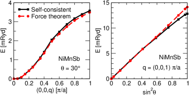
Figure 1: (color online) Comparison of the force theorem with self-consistent calculations for NiMnSb. Left: a dispersion curve of a spin spiral along the [001] direction for a cone angle $\theta=30^{\rm o}$. Right: spin spiral energy vs. $\sin^{2}\theta$ for a short-wavelength spiral along the [001] direction.

The approximation is expected to be better for smaller perturbations, i.e., for smaller cone angles and/or smaller magnon wavevectors $|\bm{q}|$. As a test, in the left panel of Figure 1 the dispersion curve is shown for a spin spiral in NiMnSb, defined by a cone angle $\theta=30^{\rm o}$, and a spin-wave vector along [001] direction. The force-theorem and self-consistent calculations agree rather well. The right panel of Fig. 1 shows the dependence of the magnon energy on the squared sinus of the cone angle ($\sin^{2}\theta$) for a fixed spin-spiral vector $\bm{q}=(0,0,1)\pi/a_{\rm lat}$. We see a a maximal deviation of the order of 7-8% for the unfavourable case of $\theta=90^{\rm o}$ and $q=\pi/a_{\rm lat}$, while the deviation starts becoming visible at cone angles larger than $\theta_{\rm max}\sim 50^{\rm o}$.

A general conclusion is that if one wants to use the force theorem to obtain the spin-spiral dispersion within the whole first Brillouin zone of the crystal, a cone angle $\theta=30^{\rm o}$ seems to be a reasonable choice, since the energy differences are not too large for the magnon to stop being a small perturbation, but are also not too small so that one would have to employ a very large basis, or $\bm{k}$-point set. This cone angle was used in the calculation of the Heisenberg interaction constants $J$ presented in Section III.

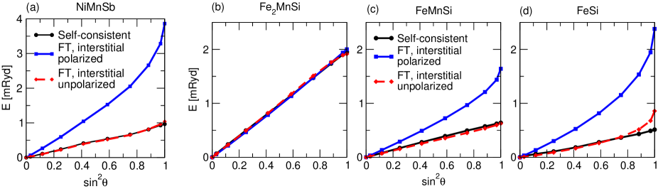
Figure 2: (color online) (a): Spiral energy $E(\bm{q},\theta)$ as function of $\sin^{2}\theta$ in NiMnSb for the cases of (i) a self-consistent calculation (including the self-consistent, spiraling polarization of the interstitial) (ii) a force-theorem calculation including the polarization of the interstitial, and (iii) a force-theorem calculation excluding the polarization of the interstitial. Evidently, case (ii) stongly overestimates the spiral energy, since the interstitial polarization acts as an effective magnetic field. Case (iii) on the other hand is a good approximation to the exact result (i). The spiral wavevector is $\bm{q}=(0,0,0.15)\,(\pi/a_{\rm lat})$. (b,c,d): Same as in (a) but for Fe₂MnSi, FeMnSi, and FeSi, in full-Heusler, half-Heusler, and zinc-blende structures, respectively, to demonstrate the effect of increasing the volume of the interstitial. The structures correspond to an fcc lattice with four, three, and two atoms per unit cell, respectively. All three were calculated in the same lattice parameter ($a_{\rm lat}=5.663$ Å) and at a spiral vector of $\bm{q}=(0,0,0.25)\,(\pi/a_{\rm lat})$.

We close this section with a comment on a spurious effect of the exchange-correlation field in the interstitial region when the force theorem is used. (The interstitial region is covered by empty spheres or empty cells in some ab-initio methods, e.g. in the ASWSandratskii02 ; Kubler06 or LMTO method,Halilov98 if the structures are relatively open, as are for instance the half-Heusler or the zinc-blende structure.) In a force-theorem application, the trial exchange-correlation potential in the interstitial is a smooth periodic function. However, in a self-consistent spin-spiral calculation, the resulting exchange-correlation potential is in many cases a much less smooth, although still periodic, function.Bylander98 Then the interstitial magnetization in the force-theorem calculation can cause a serious overestimation of the spin-spiral energy. This spurious energy contribution can be circumvented by setting the magnetic part of the exchange-correlation potential in the interstitial to zero. Depending on the volume filling of the touching “muffin-tin” atomic spheres of the system, the spurious energy can be considerable, becoming larger for open systems. In Fig. 2a we show a calculated example for NiMnSb. The self-consistent spiral energy and the force-theorem energy (here normalized to $\sin^{2}\theta$) are practically identical, if we set $\bm{B}^{xc}=0$ in the interstitial in the force theorem calculation (in the self-consistent calculation, $\bm{B}^{xc}$ is non-zero also in the interstitial); if this correction is not used, then the spiral energy is strongly overestimated. Figs. 2b-d show the same for Fe₂MnSi in the full-Heusler structure, FeMnSi in the half-Heusler structure, and FeSi in the zincblende structure. All three structures are based on an fcc lattice and were calculated here with the same lattice parameter $a_{\rm lat}=5.663$ Å, but differ in the number of atoms in the unit cell and therefore in the volume of the interstitial region. Fe₂MnSi has the smallest interstitial region, and evidently the interstitial magnetization has almost no effect; both force theorem calculations practically coincide with the self-consistent result. For FeMnSi, however, the interstitial volume is larger and the spiral energy is strongly overestimated in the force theorem calculation, if the interstital magnetization is not set to zero. The effect is even stronger for FeSi, where the interstitial volume is largest.

III Exchange Interaction Parameters and Curie Temperature

Following the prescription of Sec. II we calculated Heisenberg exchange interaction parameters ($J_{ij}$; $i,j$ are abbreviations of ${m\alpha},{n\beta}$) of Co₂MnSi and NiMnSb, shown in Fig. 3 and used a Monte Carlo method to obtain an estimate of the Curie temperatures for these compounds. The calculations for both compounds were performed within the generalized gradient approximationPBE on a 4096 $\bm{k}$-point mesh with 2744 $\bm{q}$-points in the full Brillouin zone. The planewave cutoff was $k_{\mathrm{max}}=3.8\ \mathrm{au}^{-1}$. The convergence was checked with respect to the above parameters.

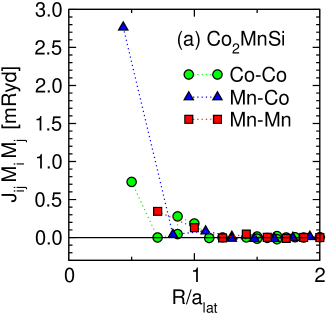
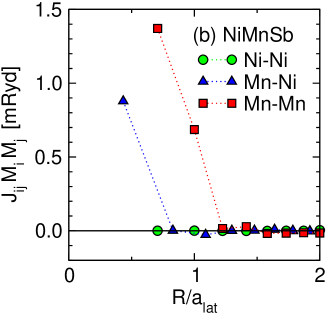
Figure 3: (color online) Heisenberg exchange interaction parameters of Co₂MnSi (a) and NiMnSb (b) as a function of the distance R between the atoms (in units of the lattice constant $a_{\rm lat}$). The lines are guides to the eye.

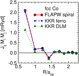
Figure 4: Heisenberg exchange interaction parameters of fcc Co as a function of the distance R between the atoms (in units of the lattice constant a). The lines are guides to the eye. Red circles: results calculated with the FLAPW method. Blue diamonds: results calculated with the Korringa-Kohn-Rostoker (KKR) Green function method within the approximation of infinitesimal rotations with the ferromagnetic state as reference. Green triangles: results calculated again with KKR but with the disordered local moment (DLM) state as reference.

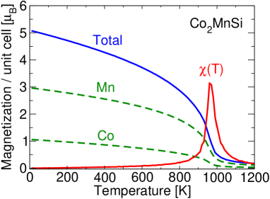
Figure 5: (color online) Magnetic moment $M(T)$ per unit cell (blue full line), partial moment of the Mn and Co sublattices (green dashed lines), and susceptibility $\chi(T)$ (red full line) as functions of the temperature $T$, for Co₂MnSi. The peak of the susceptibility at 980 K indicates the Curie temperature (experimentally found to be 985 K). Note that the susceptibilities are shown in an arbritary scale.

In Co₂MnSi, both Co and Mn atoms have strong and stable magnetic moments, whose interaction is described with $J$ parameters depicted in Fig. 3a. In NiMnSb, though the magnetic moment of Ni is small and actually induced by the Mn surrounding atoms, both Ni and Mn were treated as magnetic atoms and the parameters of Mn-Mn, Ni-Ni, and Mn-Ni interaction were calculated (Fig. 3b). As will be discussed in Sec. IV, this treatment gives an insight into the thermal behaviour of the Ni sublattice and with the use of an extended Heisenberg model more useful information can be obtained.

Co₂MnSi and NiMnSb are half-metallic ferromagnets, i.e., the density of states (DOS) in one spin direction (here majority spin) is metallic, while in the other spin direction the DOS shows a band gap around the Fermi level.

For a non-half-metallic ferromagnet, the interaction constants $J_{ij}$ as a function of distance follow a decaying oscillating behavior that in the simplest case is of the Ruderman-Kittel-Kasuya-Yoshida (RKKY) type, decaying with $|\bm{R}_{i}-\bm{R}_{j}|^{-3}$, but in general can have many superimposed periods and a different decay power law depending on the details of the Fermi surface.Pajda01 On the other hand, for half-metallic ferromagnets the gap at one spin direction leads to an imaginary wave vector and an exponential decay with distance.Pajda01 In both cases shown in Fig. 3, we notice this very fast decay of the interaction parameters with the distance between the atoms. For a comparison, in Fig. 4, the exchange interaction parameters of fcc Co (which is not half-metallic) are shown. The decay here is much slower.

In a short digression, we compare the results of the spin-spiral approach within the FLAPW method to the approach of infinitesimal rotationsLiechtenstein87 calculated with the full-potential Korringa-Kohn-Rostoker Green function method (KKR).KKR In KKR we use both the ferromagnetic state and the disordered local moment (DLM) state as reference points (see also the discussion in Sec. V.2). We see in Fig. 4 that the agreement is good for fcc Co, with a deviation of 3% nearest-neighbor coupling, if the ferromagnetic state is used as a reference, while the deviation is large if the DLM state is used as reference (also the atomic moment decreases from 1.65 $\mu_{\mathrm{B}}$ in the ground state to 1.08 $\mu_{\mathrm{B}}$ in the DLM state). For Co₂MnSi (not shown here) we find that the difference between KKR and FLAPW is larger, with the Mn-Co nearest-neighbor coupling being approximately 10% weaker in the KKR calculation, while if the DLM state is used as reference, the Co moment vanishes altogether.

Once the exchange interactions are known, the effective Heisenberg model can be solved for the Curie temperature. While the mean field approximation is computationally the simplest method to this task, it is known (and has been shown in practice) that the resulting $T_{\mathrm{C}}$ is overestimated. The random phase approximation (also known as Tyablikov approximation), on the other hand, is rather accurate.RPA The most accurate, but numerically more expensive, way to calculate $T_{\mathrm{C}}$ of a classical Heisenberg model is the Monte Carlo method, in particular when taking advantage of the cumulant expansion to account for the finite size of the simulation supercells. In this work we applied the Monte Carlo method, locating $T_{\mathrm{C}}$ by the peak in the temperature-dependent, static susceptibility. As the simulation supercells are rather large, finite-size corrections to $T_{\mathrm{C}}$ are small.

We also show Monte Carlo magnetization curves for Co₂MnSi in Fig. 5.Mersene The classical Heisenberg Hamiltonian, Eq. (1) was used to model the systems, assuming that the magnetic moments can change their orientation, but not their length. NiMnSb is discussed in more detail in Sec. IV. In the calculations the Metropolis method was employed. A supercell of 2048 unit cells (4096 magnetic atoms) was used for NiMnSb and one of 2197 unit cells (6591 magnetic atoms) for Co₂MnSi; interactions to neighbors up to a distance of four lattice constants were included. For each temperature the number of Monte Carlo sampling events was 5000, after allowing an initial relaxation time of 1000 steps and taking one sampling event every 10 sweeps of the lattice.

The magnetization curves (Fig. 5) do not go to a sharp zero at $T_{\mathrm{C}}$, but rather have a tail, as a result of the finite supercell. The peak of the susceptibility is, on the other hand, rather sharp and its position can be used to determine the Curie temperature. From the positions of these peaks, we estimated for Co₂MnSi (Fig. 5, left) $T_{\mathrm{C}}$=980 K (experimentalLandolt 985 K), and for NiMnSb (see Sec. IV) $T_{\mathrm{C}}$=870 K (experimentalLandolt value being 730 K). Note that here, for NiMnSb, the Ni moment was also taken into account within the Heisenberg model (but see also the discussion in Sec. IV, in particular IV.3). For fcc Co we find a Curie temperature of 1200 K, while the experimental result is 1403 K (the high-temperature stable phase of Co is fcc).

IV Consideration of Longitudinal Moment Fluctuations

So far we have discussed a formalism and examples of calculation of exchange parameters for a Heisenberg model, assuming that the magnitude of the local magnetic moments is rigid. However, as is long known, certain systems are weakly magnetic and the moment formation takes place at a relatively low energy scale, comparable to the magnon energies. Moriya’s quantum mechanical spin fluctuation theoryMoriya79 already factors in these effects. An introduction of a classical Hamiltonian including longitudinal and transverse degrees of freedom has been done by Uhl and KüblerUhl96 by parametrizing ab-initio total energy results; thermodynamic quantities were then obtained within a mean-field approach which coupled longitudinal and transverse degrees of freedom.Uhl96 ; Kubler06 More elaborate approaches by a classical fit of the energy to density-functional results, including transversal and longitudinal degrees of freedom, together with Monte-Carlo or classical spin-dynamics calculations, were presented e.g. by Rosengaard and Johansson,Rosengaard97 Ruban et al.,Ruban07 Ma and Dudarev,Ma12 or Derlet.Derlet12

Particularly interesting are compounds of a strongly magnetic and a weakly magnetic subsystem, where the weak moments cannot be treated as having rigid-magnitude, but on the other hand are large enough that they cannot be neglected. Examples are FePt, FePd, or NiMnSb, where the strongly magnetic atoms are Fe and Mn, while the weakly magnetic atoms are Pt, Pd and Ni. Then the assumption of rigid Heisenberg spins does no longer seem plausible. One way to circumvent this is to use only the strong magnetic moments as independent variables, but with their pair exchange parameters renormalized by the exchange among the weakly magnetic atoms and by the enhanced susceptibility. Such an approach was, for example, used by Mryasov et al.Mryasov05 ; Mryasov05b to model the temperature dependence of the magnetic anisotropy in FePt. Sandratskii et al.Sandratskii07 also find improvement in the theoretical results if the weak moments are not treated as independent, rigid Heisenberg spins, but rather fully adjust to the magnetization of the strong-moment sublattice. There is, however, the point of view of treating the weak moments not as fully enslaved to their strong-moment environment, but as independent degrees of freedom whose fluctuation can affect the thermodynamics. This point of view has been pushed for example in order to understand the antiferromagnetic-to-ferromagnetic transition of FeRh.Gruner03 ; Sandratskii11

In this section we develop a method of treating such systems, emphasizing the choise of the energetically relevant magnetic degrees of freedom at temperatures up to the critical temperature, as well as the practical implementation of these degrees of freedom to models that can be solved via Monte Carlo simulations. The additional challenge, compared to the theory developed in the previous sections, stems from two facts. First, a treatment of the weak moments as independent degrees of freedom must include the energy scale of the moments magnitude as well as their direction. Second, if the interactions of the strong moments are calculated as described earlier, by considering non-collinear magnetic configurations, then the calculated energies include a spurious contribution because the magnitude of the weak moments changes during the application of the non-collinear constraint. This spurious contribution must be accounted for. However, at the end we see that, in certain commonly occuring situations, the degrees of freedom of the weak-moment atoms can be eliminated in the statistical-mechanical calculations by using renormalized exchange parameters, while the statistical averages of the weak moments follow directly from the averages of the strong moments. We show that this is an exact result if the weak degrees of freedom give only quadratic contributions to the energy. Here we make a step-by-step approach for the special case where the weak moments do not interact with each other, while we present the more general case when they interact in the Appendix.

IV.1 General approach

The magnetically strong atoms are the main carriers of spin moment that also acts as an effective field $\bm{H}^{\rm eff}$ polarizing the magnetically weak atoms. The polarization of the latter is strengthened by an enhanced local susceptibility, which (neglecting complications from the band-structure) is $\chi=\chi_{\rm Pauli}/(1-I\chi_{\rm Pauli})$ (with $\chi_{\rm Pauli}$ the Pauli paramagnetic susceptibility and $I$ the exchange integral). Let us denote by $\bm{M}$ the rigid-magnitude local moment of the magnetically strong atoms and by $\bm{\mu}$ the supple local moment of the magnetically weak atoms. A simple expression that parametrizes the energy in terms of the local moment $\bm{\mu}$ and the polarizing field $\bm{H}^{\rm eff}$ is

$$E_{\rm loc}[\bm{H}^{\rm eff},\bm{\mu}]=-\bm{H}^{\rm eff}\cdot\bm{\mu}+a\mu^{2}+b\mu^{4}$$ (14)

It is implied that $\bm{H}^{\rm eff}=\kappa\sum_{n\in\rm neighb}\bm{M}_{n}+\bm{H}^{\rm ext}$, where $\bm{M}_{n}$ is the summed moment of the neighboring atoms inducing a polarization, $\kappa$ is a phenomenological parameter which encapsulates all microscopic processes (in particular electron hoppings) that couple $\bm{\mu}$ to $\bm{M}_{n}$, while $\bm{H}^{\rm ext}$ is an external magnetic field that we henceforth set to zero.footnote In the absence of a field $\bm{H}^{\rm eff}$ Eq. (14) contains only even powers of $\bm{\mu}$, because symmetry requires $E_{\rm loc}[0,\bm{\mu}]=E_{\rm loc}[0,-\bm{\mu}]$.

In Eq. (14) we always must have $b\geq 0$. The case of spontaneous polarization is described by $a<0$ and $b>0$, while the case of induced magnetic moments is described by $a>0$. In this case, the on-site susceptibility is

$$\chi=\partial\mu/\partial H^{\rm eff}|_{H^{\rm eff}=0}=1/(2a).$$ (15)

Thus the enhancement of the susceptibility is contained in the parameter $a$.

Eq. (14), if the fourth-order term is negligible, can be written as

$$E_{\rm loc}[\bm{H}^{\rm eff},\bm{\mu}]=a\biggl{(}\bm{\mu}-\frac{1}{2a}\bm{H}^{\rm eff}\biggr{)}^{2}-\frac{1}{4a}(H^{\rm eff})^{2},\ \text{if $b=0$.}$$ (16)

To elaborate on these ideas we use NiMnSb as a concrete example. In this case the Mn subsystem is magnetically strong and the Ni subsystem magnetically weak. We have also found that in this case it is a good approximation to set $b=0$ (as we show below), which we adopt. Combining Eq. (14) at $b=0$ with the Heisenberg-model energy expression for the Mn subsystem results in the extended model Hamiltonian

$$\mathcal{H}(\{\bm{M}_{i};\bm{\mu}_{l}\}) = -\frac{1}{2}\sum_{ij\in{\rm Mn}}J^{b}_{ij}\bm{M}_{i}\cdot\bm{M}_{j}$$ (17)

$$+ \sum_{l\in\rm Ni}[a\mu_{l}^{2}-\kappa\bm{\mu}_{l}\cdot\sum_{n(l)}\bm{M}_{n}]$$

where $\sum_{n(l)}\bm{M}_{n}$ is the sum of the moments of the Mn nearest neighbors of the $l$-th Ni atom, $n(l)$, and $\bm{M}_{i}$ and $\bm{\mu}_{l}$ refer to the Mn and Ni moment respectively. The superscript “$b$” in the Mn-Mn exchange interaction is placed in anticipation that it does not coincide with the quantity calculated within the method presented in Sec. II, but with a “bare” quantity, as will be discussed below. It has been also assumed that the Ni-Ni interaction can be neglected, as there are no Ni-Ni nearest neighbor pairs, while from the calculations it becomes evident that more distant Ni-Ni interactions are negligible (the case where the interactions among the weak-sublattice moments are non-negligible is discussed in the Appendix). The above equation can be rewritten in a somewhat more convenient form, if we define (with an obvious notation)

$$J^{b}_{{\rm Mn}-\rm Ni} = \left\{\begin{array}[]{ll}\kappa,&\text{nearest neighbours Mn-Ni}\\ 0,&\text{otherwise}\end{array}\right.$$ (20)

$$J_{\rm Ni-\rm Ni} = 0$$ (21)

Then Eq. (17) takes the form

$$\mathcal{H} = -\frac{1}{2}\bigg{[}\sum_{ij\in{\rm Mn}}J^{b}_{ij}\bm{M}_{i}\cdot\bm{M}_{j}+\sum_{i\in{\rm Mn},l\in\rm Ni}J^{b}_{il}\bm{M}_{i}\cdot\bm{\mu}_{l}$$

$$+\sum_{j\in{\rm Mn},l\in\rm Ni}J^{b}_{lj}\bm{\mu}_{l}\cdot\bm{M}_{j}\bigg{]}+\sum_{l\in\rm Ni}a\mu_{l}^{2}$$

This form is appealing, as it contains a Heisenberg-like expression among all magnetic atoms plus a local correction term that accounts for the longitudinal degree of freedom of the Ni moments. However, it is important to remember that the Ni moments included in the scalar products of the RHS can change in size as well as angle, deviating from the traditional Heisenberg model.

We can derive the parameters $\kappa$ and $a$ from DFT calculations as follows. From Eq. (16) it follows that the equilibrium value of the Ni moment at $T=0$ and for zero external field is linearly dependent to the polarizing neigboring Mn moments:

$$\mu_{\rm eq}=\frac{\kappa}{2a}N_{c}\,M$$ (23)

where $N_{c}=4$ is the coordination number of a Ni atom with respect to Mn neighbors. From this expression one can deduce the ratio $\kappa/a$ once $M$ and $\mu_{\rm eq}$ have been calculated in the ferromagnetic state by an ab-initio method. On the other hand, $a$ can be determined by introducing into the DFT calculation a constraint on the Ni moment, either in the form of a longitudinal magnetic field constraining the magnitude or in the form of a transverse magnetic field constraining the angle $\theta$ of $\bm{\mu}$ with respect to the moment directions at the Mn neighbors, but allowing the magnitude to relax to $\mu_{\rm eq}(\theta)$. The former method results in a parabolic (for $b=0$) moment-dependence of the total energy, as suggested by Eqs. (14,16). The latter method results in the following dependence, as can be easily found by an energy minimization of Eq. (16) at a given $\theta$:

$$\mu_{\rm eq}(\theta) = \mu_{\rm eq}(0)\cos\theta$$ (24)

$$E_{\rm loc}(\theta)-E_{\rm loc}(0) = a(\bm{\mu}_{\rm eq}(\theta)-\bm{\mu}_{\rm eq}(0))^{2}$$ (25)

$$= a\mu_{\rm eq}(0)^{2}\sin^{2}\theta.$$

If the extended Heisenberg model provides a good approximation to the energetics of the system, then Eqs. (16) and (25) should both yield a good approximation to the calculated DFT energy difference, when a constraint is applied on the Ni moment, and the extracted parameter $a$ for the two cases should be approximately the same. We find that this is the case in NiMnSb (see Fig 6).footnote1 This allows us to extract the value of $a$ from the DFT calculation and from this the value of $\kappa$ (equivalent to $J^{b}_{{\rm Mn}-\rm Ni}$) via Eq. (23). Thus the ingredients of formula (LABEL:eq:L3) are accessible.

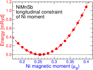
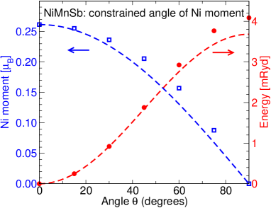
Figure 6: (color online) Top: Dependence of the total energy on the Ni moment in NiMnSb under the constraint of an external field acting on the Ni atoms. Circles: calculated data (within DFT). Dashed curve: parabolic fit to Eq. (16) with $a=53{\rm mRyd}/\mu_{\mathrm{B}}^{2}$. Bottom: Dependence of the Ni moment and the total energy on the constraining angle $\theta$ tilting the Ni moment away from the Mn moment in NiMnSb. Blue squares: $\mu_{\rm eq}(\theta)$ (scale displayed on the left-side ordinate). Red circles: $E_{\rm DFT}(\theta)-E_{\rm DFT}(0)$ (scale displayed on the right-side ordinate). The broken lines correspond to fits to Eqs. (24) and (25). In the energy fit, the last part of Eq. (25) was used with the prefactor $a=55.3{\rm mRyd}/\mu_{\mathrm{B}}^{2}$ fitted to the low-angle contributions ($\theta=15^{\circ}$ and $30^{\circ}$).

There remains, however, a correction to be made, connected to a “renormalization” of the Mn-Mn exchange constants which have been calculated within the spin-spiral method described in Section II. To clarify the problem we remind the reader that, when calculating spin spirals, one normally constrains the direction of the moments but not their magnitude. For the Ni atoms, where the rigid-moment approximation is not valid, the magnitude $\mu$ is reduced by the spin-spiral formation due to the canting of the neighboring Mn moments in different directions. This effect provides an additional, indirect energy contribution to the spin spiral and to the Mn-Mn interaction, compared to the case that the Ni-moments magnitude would have been kept constant. It is the spurious contribution that we mentioned in the introduction to Sec. IV. Let us call this contribution $J_{{\rm Mn}-\rm Ni-{\rm Mn}}$. The calculated Mn-Mn interaction consists thus of two parts:

$$J_{{\rm Mn}-{\rm Mn}}=J^{b}_{{\rm Mn}-{\rm Mn}}+J_{{\rm Mn}-\rm Ni-{\rm Mn}},$$ (26)

with $J^{b}_{{\rm Mn}-{\rm Mn}}$ the sought-after bare interaction entering Eqs. (20) and (LABEL:eq:L3), while $J_{{\rm Mn}-{\rm Mn}}$ is a renormalized interaction that is probed by the spin-spiral DFT calculation. For more distant Mn atoms, which have no common Ni neighbor, $J^{b}_{{\rm Mn}-{\rm Mn}}$ coincides with $J_{{\rm Mn}-{\rm Mn}}$.

For the derivation of an expression, e.g. in the case of NiMnSb, giving $J_{{\rm Mn}-\rm Ni-{\rm Mn}}$, consider $N_{c}(=4)$ Mn atoms as nearest neighbors of a Ni atom. Then the local-energy expression (16) becomes

$$E_{\rm loc} = -\kappa\sum_{n=1}^{N_{c}}\bm{M}_{n}\cdot\bm{\mu}+a\mu^{2}$$ (27)

$$= -\frac{1}{2}\sum_{n,n^{\prime}=1}^{N_{c}}\frac{\kappa^{2}}{2a}\bm{M}_{n}\cdot\bm{M}_{n^{\prime}}-\frac{\kappa^{2}}{4a}N_{c}\,M^{2}$$

Here, $n$ and $n^{\prime}$ run through the Mn moments. The second step follows under the condition that, in the DFT calculation, the Ni moment relaxes to the particular equilibrium value that is dictated by the neighboring Mn-moment directions, i.e., $\bm{\mu}=\frac{\kappa}{2a}\sum_{n}\bm{M}_{n}$. From Eq. (27) we obtain the indirect interaction:

$$J_{{\rm Mn}-\rm Ni-{\rm Mn}}=-\frac{\delta^{2}E_{\rm loc}}{\delta\bm{M}_{n}\delta\bm{M}_{n^{\prime}}}=\frac{\kappa^{2}}{2a}$$ (28)

At this point it is important to note that, whether one chooses to work with $J_{{\rm Mn}-{\rm Mn}}$ or $J^{b}_{{\rm Mn}-{\rm Mn}}$, depends on the choice of the degrees of freedom. If only the Mn moments are chosen as degrees of freedom, then $J_{{\rm Mn}-{\rm Mn}}$ has to be used. If, however, the Ni moments are also chosen as independent degrees of freedom, then $J^{b}_{{\rm Mn}-{\rm Mn}}$ has to be used together with $J^{b}_{{\rm Mn}-\rm Ni}=\kappa$. In the latter case, according to the prescription leading to Eqs. (20) and (28), we arrive at the extended Heisenberg Hamiltonian (LABEL:eq:L3) with the appropriate bare parameters in the nearest-neighbor coupling.

IV.2 Analytical elimination of weak degrees of freedom at $T>0$

In the previous subsection we discussed the bare and renormalized parameters of the model arising from total-energy calculations of the constrained ground state. In this section we examine the case of thermodynamic quantities at $T>0$, where it is not a priori obvious that the same renormalization is still valid if the weak moments are allowed to fluctuate. We find that, in the absence of fourth order terms in $E_{\rm loc}$ [$b=0$ in Eq. (14)], also at $T>0$ the weak moments can be eliminated in favour of the same renormalized parameters as the ones appearing at $T=0$. Our conclusion is based on an exact analytical integration of the weak-moment part of the partition function in the case $b=0$.

First we observe that the energy functional (16) under the action of $\bm{H}^{\rm eff}$ has the same quadratic form as the one with $\bm{H}^{\rm eff}=0$, only with the minimum shifted to $\bm{\mu}_{\rm eq}=\bm{H}^{\rm eff}/(2a)$. This simplifies the integration of the partition function. To see this, we first transform the Hamiltonian (17) in such a way that the renormalized interactions $J_{ij}$ appear explicitly. We start by rewriting Eq.  (17) as:

$$\mathcal{H}(\{\bm{M}_{i};\bm{\mu}_{l}\}) = -\frac{1}{2}\sum_{ij}J^{b}_{ij}\bm{M}_{i}\cdot\bm{M}_{j}$$ (29)

$$+a\sum_{l}\left(\bm{\mu}_{l}-\frac{\kappa}{2a}\sum_{n(l)}\bm{M}_{n}\right)^{2}$$

$$-\frac{\kappa^{2}}{4a}\sum_{l}(\sum_{n(l)}\bm{M}_{n})^{2}$$

The indices $i,j$ run over the Mn atoms, the index $l$ over the Ni atoms, and $n(l)$ over the Mn neighbours of the $l$-th Ni atom. The last term is now split in an interatomic contribution and an on-site contribution:

$$-\frac{\kappa^{2}}{4a}\sum_{l}(\sum_{n(l)}\bm{M}_{n})^{2}=$$

$$-\frac{1}{2}\sum_{l}\sum_{\begin{subarray}{c}n(l),n^{\prime}(l)\\ n\neq n^{\prime}\end{subarray}}\frac{\kappa^{2}}{2a}\bm{M}_{n}\cdot\bm{M}_{n^{\prime}}+\sum_{l}\sum_{n(l)}\frac{\kappa^{2}}{2a}M_{n}^{2}$$

$$=-\frac{1}{2}\sum_{ij;i\neq j}\frac{\kappa^{2}}{2a}c(i,j)\bm{M}_{i}\cdot\bm{M}_{j}+\sum_{l}\sum_{n(l)}\frac{\kappa^{2}}{2a}M_{n}^{2}$$ (30)

In the last step we have converted the sum $\sum_{l}\sum_{\begin{subarray}{c}n\end{subarray}(l),n^{\prime}(l)\\ n\neq n^{\prime}}$ to a sum over $i,j$, by introducing a combinatorial factor $c(i,j)$ that counts how many common Ni neighbors the $i$-th and $j$-th Mn atoms have. From the structure of NiMnSb it follows that $c(i,j)=1$, if $i,j$ are nearest-neighbors in the Mn fcc sublattice (i.e. if the distance between $i$ and $j$ is $a_{\rm lat}/\sqrt{2}$) and $c(i,j)=0$ otherwise. Actually we have recovered the quantity $J_{{\rm Mn}-\rm Ni-{\rm Mn}}=\kappa^{2}/(2a)$ of Eqs. (27) and (28). Finally, the last term of Eq. (30) is just a constant which can be omitted. Using the definition (26) and Eq. (28), we combine the first term of the RHS of Eq. (29) with the first term of the RHS of Eq. (30) to obtain the renormailized $J_{ij}$. Then the Hamiltonian to be used in the partition function takes the form:

$$\mathcal{H}(\{\bm{M}_{i};\bm{\mu}_{l}\}) = -\frac{1}{2}\sum_{ij}J_{ij}\bm{M}_{i}\cdot\bm{M}_{j}+a\sum_{l}\left(\bm{\mu}_{l}-\frac{\kappa}{2a}\sum_{n(l)}\bm{M}_{n}\right)^{2}$$ (31)

$$= \mathcal{H}_{r}+a\sum_{l}\left(\bm{\mu}_{l}-\frac{\kappa}{2a}\sum_{n(l)}\bm{M}_{n}\right)^{2}$$

where the Heisenberg Hamiltonian involving only the Mn sublattice with the renormalized interactions, $\mathcal{H}_{r}=-\frac{1}{2}\sum_{ij}J_{ij}\bm{M}_{i}\cdot\bm{M}_{j}$, has been introduced for convenience as part of the full Hamiltonian. Note that there is no renormalization for the Ni-Mn interactions: either they should be completely omitted within $\mathcal{H}_{r}$ that includes only the Mn moments, or they should be given by Eq. (20) in the generalized model. The spin-spiral result for $J_{{\rm Mn}-\rm Ni}$ does not enter in our theory.

The partition function is:

$$\mathcal{Z} = \int d\Omega_{1}\cdots d\Omega_{N}\int d^{3}\mu_{1}\cdots d^{3}\mu_{N}\exp\left\{-\frac{\mathcal{H}(\{\bm{M}_{i};\bm{\mu}_{l}\})}{k_{B}T}\right\}$$ (32)

$$= \int d\Omega_{1}\cdots d\Omega_{N}\exp\left\{-\frac{\mathcal{H}_{r}}{k_{B}T}\right\}\int d^{3}\mu_{1}\cdots d^{3}\mu_{N}\exp\left\{-\frac{a\sum_{l}(\bm{\mu}_{l}-\frac{\kappa}{2a}\sum_{n(l)}\bm{M}_{n})^{2}}{k_{B}T}\right\}$$ (33)

$$= \int d\Omega_{1}\cdots d\Omega_{N}\exp\left\{-\frac{\mathcal{H}_{r}}{k_{B}T}\right\}\left(\frac{\pi k_{B}T}{a}\right)^{\frac{3N}{2}}$$ (34)

$$= \mathcal{Z}_{r}\left(\frac{\pi k_{B}T}{a}\right)^{\frac{3N}{2}}$$ (35)

where $\int d\Omega_{1}\cdots d\Omega_{N}$ denotes an integration over the Mn-moment solid angles. The integration over the Ni-moments $\int d^{3}\mu_{1}\cdots d^{3}\mu_{N}$ contains only the exponential of a complete square and has been analytically integrated to $(\pi k_{B}T/a)^{3N/2}$, i.e., it corresponds to the partition function of $3N$ uncoupled harmonic degrees of freedom and is independent of the value of $\bm{M}_{n}$. $\mathcal{Z}_{r}$ is the partition function corresponding to the Hamiltonian $\mathcal{H}_{r}$. The magnetization $\langle\bm{M}\rangle$ of the Mn sublattice also turns out to depend only on the renormalized partition function (and Hamiltonian). The same is true for any moment-moment correlation function of the Mn sublattice, $\langle(M_{1x})^{m_{1x}}(M_{1y})^{m_{1y}}\cdots(M_{Nz})^{m_{Nz}}\rangle$, $\alpha\in(x,y,z)$, where the $m_{n\alpha}\geq 0$ are integer exponents defining the order of the correlation function. To see this we consider explicitly

$$\langle(M_{1x})^{m_{1x}}(M_{1y})^{m_{1y}}\cdots(M_{Nz})^{m_{Nz}}\rangle = \frac{1}{\mathcal{Z}}\int d\Omega_{1}\cdots d\Omega_{N}(M_{1x})^{m_{1x}}\cdots(M_{Nz})^{m_{Nz}}\exp\{-\mathcal{H}_{r}/k_{B}T\}$$ (36)

$$\times\int d^{3}\mu_{1}\cdots d^{3}\mu_{N}\exp\biggl{\{}-\frac{a\sum_{l}(\bm{\mu}_{l}-\frac{\kappa}{2a}\sum_{n(l)}\bm{M}_{n})^{2}}{k_{B}T}\biggr{\}}$$

$$= \frac{1}{\mathcal{Z}_{r}}\int d\Omega_{1}\cdots d\Omega_{N}(M_{1x})^{m_{1x}}\cdots(M_{Nz})^{m_{Nz}}\exp\{-\mathcal{H}_{r}/k_{B}T\}$$ (37)

where the Hamiltonian in the exponential has again been split in two terms according to Eq. (31) and the integration over $d^{3}\mu_{1}\cdots d^{3}\mu_{N}$ has again been carried out analytically, cancelling out the factor $(\pi k_{B}T/a)^{3N/2}$ in the full partition function. But expression (37) is just the expression for the correlation function of only the Mn sublattice with the renormalized Heisenberg interactions. Thus we see that, as far as the Mn-sublattice magnetization is concerned, one can use the exchange interactions calculated by the spin-spiral method that are renormalized by construction, while neglecting the Ni moments and the Mn-Ni interaction. If the Ni moments are to be included, then the bare interactions have to be used in an extended model, however, the Mn-sublattice properties in the two cases will be the same. Note, finally, that this exact result is based on the fact that the exponent in the integration over $d^{3}\mu_{1}\cdots d^{3}\mu_{N}$ contains a complete square, i.e., that the “harmonic” approximation, $b=0$, is valid; if $b\neq 0$ and one proceeds to an elimination of the weak degrees of freedom, then the resulting renormalized strong-moment Hamiltonian can have higher-order terms (biquadratic, four-spin, etc.) with temperature-dependent parameters.

A semi-analytical result follows in an analogous way also for the average Ni moment and fluctuation amplitude per atom:

$$\langle\bm{\mu}\rangle = \frac{\kappa}{2a}N_{c}\,\langle\bm{M}\rangle$$ (38)

$$\langle\mu^{2}\rangle := \frac{1}{N}\langle[\sum_{l=1}^{N}\bm{\mu}_{l}]\rangle^{2}$$

$$= \frac{1}{a}\frac{3}{2}k_{B}T+\left(\frac{\kappa}{2a}N_{c}\right)^{2}\frac{1}{N}\langle[\sum_{i=1}^{N}\bm{M}_{i}]^{2}\rangle$$

$$= \frac{1}{a}\frac{3}{2}k_{B}T+\left(\frac{\kappa}{2a}N_{c}\right)^{2}\langle M^{2}\rangle$$ (40)

I.e., there is a “harmonic” part and a part induced by the fluctuation of the Mn sublattice. The former is independent of the number of atoms, while the latter, $\langle M^{2}\rangle:=\langle[\sum_{i=1}^{N}\bm{M}_{i}]^{2}\rangle/N$, increases proportionally to the number of magnetic atoms in the system for $T<T_{\mathrm{C}}$, as in normal Heisenberg systems.footnoteHMK The longitudinal susceptibility $\chi_{\rm Ni}$ of the Ni sublattice can be found in a completely analogous way:

$$k_{B}T\,\chi_{\rm Ni} = \langle\mu_{z}^{2}\rangle-\langle\mu_{z}\rangle^{2}$$ (41)

$$= \frac{1}{a}\frac{k_{B}T}{2}+\left(\frac{\kappa}{2a}N_{c}\right)^{2}(\langle M_{z}^{2}\rangle-\langle M_{z}\rangle^{2})$$

$$= k_{B}T\left[\frac{1}{2a}+\left(\frac{\kappa}{2a}N_{c}\right)^{2}\chi_{{\rm Mn}}\right]$$ (42)

i.e., there is again a harmonic part and a part proportional to the Mn sublattice susceptibility. (In Eq. (41), $z$ is implied to be the direction of magnetization.)

According to these results, as long as the approximation $b=0$ holds, one can deduce the thermodynamic properties of the weak sublattice by merely a calculation on the strong sublattice, avoiding the extra numetical cost that a full Monte Carlo simulation entails. Actually this procedure can be carried out for higher-order correlation functions of the Ni moments, $\langle(\mu_{1x})^{m_{1x}}(\mu_{1y})^{m_{1y}}\cdots(\mu_{Nz})^{m_{Nz}}\rangle$ ($\alpha\in(x,y,z)$), where once again the $m_{l\alpha}\geq 0$ are integer exponents defining the order of the correlation function. In the resulting formula the integration over $d^{3}\mu_{l}$ can be carried out analytically, yielding a sum of correlation functions of the $\bm{M}_{i}$ of the form:

$$\langle\mu_{1x}^{m_{1x}}\cdots\mu_{Nz}^{m_{Nz}}\rangle = \frac{1}{\mathcal{Z}}\int d\Omega_{1}\cdots d\Omega_{N}e^{-\frac{\mathcal{H}_{r}}{k_{B}T}}\int d^{3}\mu_{1}\cdots d^{3}\mu_{N}(\mu_{1x})^{m_{1x}}\cdots(\mu_{Nz})^{m_{Nz}}\exp\biggl{\{}-\frac{a\sum_{l}(\bm{\mu}_{l}-\frac{\kappa}{2a}\sum_{n(l)}\bm{M}_{n})^{2}}{k_{B}T}\biggr{\}}$$ (43)

$$= \frac{1}{{\mathcal{Z}_{r}}}\int d\Omega_{1}\cdots d\Omega_{N}e^{-\frac{\mathcal{H}_{r}}{k_{B}T}}\prod_{l=1}^{N}\prod_{a\in xyz}\sum_{\begin{subarray}{c}p=0\\ p\ \rm even\end{subarray}}^{m_{l\alpha}}\binom{m_{l\alpha}}{p}(p-1)!!\left(\frac{k_{B}T}{2a}\right)^{p/2}\Bigl{(}\frac{\kappa}{2a}\sum_{n(l)}M_{n\alpha}\Bigr{)}^{m_{l}(\alpha)-p}$$

where a change of variables $\mu_{l\alpha}\rightarrow\mu_{l\alpha}+\frac{\kappa}{2a}\sum_{n(l)}M_{n\alpha}$ has been performed, the binomial expansion of $(\mu_{l\alpha}+\frac{\kappa}{2a}\sum_{n(l)}M_{n\alpha})^{m_{l\alpha}}$ has been used and we have taken into account that integrals of the type $\int_{-\infty}^{\infty}x^{p}e^{-ax^{2}}=\sqrt{\frac{\pi}{a}}(p-1)!!/(2a)^{p/2}$ for even $p$ and vanish for odd $p$ [for the $p=0$ term we accept the convention $(-1)!!=1$]. Due to the presence of products of $M_{n\alpha}$ in Eq. (43) it is clear that this expression reduces to a sum of correlation functions of the $\bm{M}_{i}$ within the Hamiltonian $\mathcal{H}_{r}$. The summations in this expression are too involved to arrive at a general closed form, however, Eqs. (38), (40) and (42) are special cases of application of this formula. Obviously, mixed correlation functions between strong and weak moments can also be reduced to strong-moment correlation functions of the renormalized Hamiltonian by first eliminating the weak moments following the same prescription.

We should stress that choosing to eliminate the weak moments in favour of renormalized interactions does not mean that the weak moments are physically less valid as degrees of freedom; to do so is merely a matter of mathematical or computational convenience, especially since efficient methods exist for the calculation of thermodynamic quantities within the classical Heisenberg model.

IV.3 Calculations in NiMnSb

We exemplify the above results with calculations in NiMnSb. First we establish which interactions can be neglected. To this end we performed calculations of the exchange coupling parameters by the spin-spiral method. As it turns out, the Ni-Ni interactions are negligible. About the Mn-Mn interactions, Fig. 3b suggests that it should be enough to include up to 2nd neigbors, but this is misleading; we find by Monte Carlo calculations a 2nd neighbor approximation leads to an overestimation of approximately 100 K in $T_{\mathrm{C}}$ compared to the value including also more distant neighbors, therefore we include Mn-Mn interactions up to a distance of three lattice parameters. Among the Mn-Ni interactions (Fig. 3b) only the nearest-neighbor coupling has some small influence, changing $T_{\mathrm{C}}$ by a modest 20 K. Given the conclusions of the previous subsection, the Mn-Ni interaction should be excluded for an estimation of $T_{\mathrm{C}}$, since the Mn-Mn interactions are already renormalized (in the corresponding spin-spiral calculations the magnitude of the Ni moment was allowed to relax). The Mn-Ni interaction must be included if one wishes to extract information on the behavior of the Ni magnetization; then, however, the interaction type and strength has to be corrected, since the Ni atoms belong to a soft-magnetic sublattice.

After deriving the exchange parameters $J_{ij}$ by the spin-spiral method, utilizing the force theorem which according to Fig. 2a is accurate enough for this purpose, we performed constrained-angle calculations for the Ni moments with full self-consistency. From the total-energy results shown in Fig. 6, together with Eq. (25), we deduce a value of $a=55.3~{}{\rm mRyd}/\mu_{\mathrm{B}}^{2}$. Given this, together with the ground-state magnetic moments of Mn $M=3.71~{}\mu_{\mathrm{B}}$ and of Ni $\mu_{\rm eq}=0.26~{}\mu_{\mathrm{B}}$, Eqs. (20) and (23) yield a value of $J^{b}_{{\rm Mn}-\rm Ni}\equiv\kappa=1.94~{}{\rm mRyd}/\mu_{\mathrm{B}}^{2}$. This bare value $J^{b}_{{\rm Mn}-\rm Ni}$ is significantly different than the value of $0.92~{}{\rm mRyd}/\mu_{\mathrm{B}}^{2}$ for the Mn-Ni interaction, which was derived from the spin-spiral calculation (Fig. 3B). Finally, from Eqs. (26) and (28) we can extract the bare value of the nearest-neighbor Mn-Mn interaction: $J_{{\rm Mn}-{\rm Mn}}^{b}=0.066~{}{\rm mRyd}/\mu_{\mathrm{B}}^{2}$, which shows a reduction of about $1/3$ compared to the corresponding renormalized value. Note that the equilibrium moments have to be multiplied to these values if comparison is to be made with the energies shown in Fig. 3B. Then one obtains $J^{b}_{{\rm Mn}-{\rm Mn}}M^{2}=0.91~{}{\rm mRyd}$ and $J^{b}_{{\rm Mn}-\rm Ni}M\mu_{\rm eq}=1.87~{}{\rm mRyd}$; i.e., the Mn-Mn bare interaction is weaker than the Mn-Ni, which is not surprising, since the Ni polarization stems from a direct, nearest-neighbor exchange interaction with Mn.

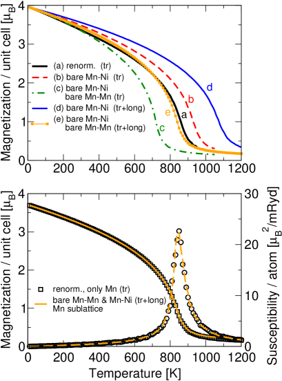
Figure 7: (color online) Top: Monte Carlo results on the magnetization of NiMnSb under various assumptions on the model and the interactions. (a-c): Only transverse fluctuations are taken. (a): Interactions as derived by force-theorem, spin-spiral calculations, including Mn-Mn and Mn-Ni. (b) Same as (a), but with bare Mn-Ni interactions $J^{b}_{{\rm Mn}-\rm Ni}$ (Eq. 17). (c) Same as (b), but additionally with bare Mn-Mn interactions $J^{b}_{{\rm Mn}-{\rm Mn}}$ (given by Eqs. (26,28)). (d-e): Also longitudinal fluctuations of the Ni-moment are allowed. (d) Bare Mn-Ni interactions. (e) Bare Mn-Ni and Mn-Mn interactions. Evidently, taking the Mn-Ni bare interaction alone leads to an overestimation of the excitation energies and $T_{\mathrm{C}}$, which is corrected when the bare Mn-Mn interaction is also taken. Bottom: Magnetization curve and susceptibility of the Mn sublattice in NiMnSb calculated within different models. Squares (magnetization) and circles (susceptibility): Only transverse fluctuations with renormalized Mn-Mn interactions, neglecting completely the Ni moments. Full line: Transverse and longitudinal fluctuations are allowed for the Ni atoms, only transverse for Mn, with bare Mn-Mn and Mn-Ni parameters; only the Mn sublattice magnetization and susceptibility is shown (i.e., corresponding to the Mn part of curve (e) in the top panel). Note on the susceptibility units that $1\mu_{\mathrm{B}}^{2}/{\rm mRyd}=4.254\times 10^{-3}\mu_{\mathrm{B}}/{\rm Tesla}$. The temperature dependence of the magnetization and susceptibility is identical in the two cases for reasons that are explained in the text.

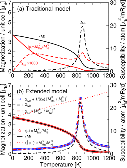
Figure 8: (color online) Magnetization curves and sublattice susceptibility in the traditional and extended model. The notation is as follows: $\langle M\rangle$ and $\langle\mu\rangle$ stand for the temperature-dependent magnetization of the Mn and Ni sublattices, respectively; $\langle|\mu|\rangle$ stands for the thermal average of the absolute value of the Ni local moment; $\chi_{\rm Mn,Ni}$ for the sublattice susceptibilities of Mn and Ni; and $M_{\rm Mn,Ni}^{0}$ for the ground-state local moments. (a) Traditional model (only transverse fluctuations of the moment) with the interactions derived by force-theorem from spin-spiral calculations. The Mn magnetization shows a typical ferromagnetic behavior with a susceptibility peak at $T_{\mathrm{C}}$. On the other hand the Ni magnetization drops rather fast, with an atypical susceptibility showing a plateau over a wide region. (b) Extended model (longitudinal fluctuations of the Ni moment are allowed) with bare Mn-Ni and Mn-Mn interactions. The Mn magnetization hardly changes compared to (a), and the $T_{\mathrm{C}}$ is very similar, but the behavior of the Ni magnetization and susceptibility are completely different, following the critical behavior of the Mn sublattice. At $T=0$, the Ni susceptibility does not vanish, behaving as it is expected for a system with non-rigid moments, reaching the value $\chi=1/(2a)=0.009~{}\mu_{\mathrm{B}}^{2}/{\rm mRyd}$ at $T=0$. The average of the magnitude of the local Ni moment increases with temperature. The Monte Carlo simulations included 2048 unit cells (4096 atoms). The Ni-related quantities have been scaled up by the annotated factors in order to demonstrate the agreement with Eqs. (38) and (42): $\langle\mu\rangle$ and $\langle|\mu|\rangle$ by a factor $M_{\rm Mn}^{0}/M_{\rm Ni}^{0}=14.2$ and $\chi_{\rm Ni}$ by $(M_{\rm Mn}^{0}/M_{\rm Ni}^{0})^{2}=201$. In particular the blue squares show the validity of Eq. (42), i.e., the derivation of the Ni from the Mn susceptibility. The latter coincides with the $\chi_{{\rm Mn}}$ of the traditional renormalized model, as is demonstrated in Fig. 7 (bottom panel).

Next we present a series of Monte-Carlo-simulation results, examining the effect and importance of the bare interactions. We performed simulations in the framework of the traditional model (only transverse fluctuations allowed) as well as the extended model (longitudinal fluctuations also allowed), with the renormalized and bare parameters. Putting it all together, we must substitute the above-found parameters $J_{{\rm Mn}-{\rm Mn}}^{b}$, $J_{{\rm Mn}-\rm Ni}^{b}$, and $a$, into the extended Hamiltonian (LABEL:eq:L3) which is to be treated with a Monte Carlo method where the (weak) Ni moments $\bm{\mu}_{l}$ should be allowed to vary in length and direction while the (strong) Mn moments should be allowed to vary in direction only. In this particular example, a distinction between bare and renormalized interactions was made only for the nearest-neighbour Mn-Mn and Mn-Ni coupling. The longer-range Mn-Ni coupling was assumed to vanish thus there can be no renormalization in the longer-range Mn-Mn coupling [as the distant Mn atoms have no common Ni neighbor, i.e., $J_{{\rm Mn}-\rm Ni-{\rm Mn}}=0$ for distant atoms in Eq. 26]. The Ni-Ni coupling was also assumed to vanish. The results are to be compared with calculations employing the traditional Hamiltonian

$$\mathcal{H}(\{\bm{M}_{i}\})=-\frac{1}{2}\sum_{ij\in{\rm Mn}}J_{ij}\bm{M}_{i}\cdot\bm{M}_{j}$$ (44)

containing only the Mn moments that vary in direction, where now $J_{ij}$ are the Mn-Mn renormalized parameters, i.e., obtained from the spin-spiral method presented in Sec. II and shown (multiplied by the moments) in Fig. 3b. In both cases the Mn-Mn interaction was included up to a distance of three lattice parameters. The first set of results is contained in Fig. 7, where magnetization curves are shown, calculated within different assumptions. Here we omit showing the susceptibiliy, but the Curie temperature can be recognized by the characteristic inflection point of the magnetization curve. The central results are included in curves (a) and (e) of the top panel, as well as in the bottom panel, while curves (b), (c) and (d) merely show that neglecting some of the degrees of freedom or some of the bare constants leads to almost arbitrary results. In the simulations including longitudinal moment fluctuations, more Monte Carlo steps were necessary, typically by an order of magnitude, in order to arrive at the same quality as in the simulations including only transverse fluctuations.

Curve (a) shows the result of the traditional model with spin-spiral-derived (i.e., renormalized) Mn-Mn exchange parameters, including spin-spiral-derived Mn-Ni interactions. This results in $T_{\mathrm{C}}=870~{}{\rm K}$. Curve (b) includes the bare Mn-Ni parameters, but stays within the traditional model. $T_{\mathrm{C}}$ increases by a modest amount of 60 K, since the bare Mn-Ni parameters are stronger than the spin-spiral-calculated ones. Curve (c) also stays within the traditional model, but includes the bare Mn-Mn interaction, which is weaker by a factor $1/3$ compared to the renormalized value; $T_{\mathrm{C}}$ drops significantly to 730 K. This coincides with the experimental value, but the coincidence is probably fortuitous: the longitudinal fluctuations at Ni, that are essential to the derivation of the bare parameters, are yet unaccounted for in the simulation (see, however, the discussion on the phase space measure in subsection V). Next comes curve (d), where the longitudinal fluctuations are allowed for in the simulation, but taking the bare Mn-Ni and the renormalized Mn-Mn exchange. The increase in $T_{\mathrm{C}}$ (1090 K) with respect to curve (b) (same parameters but rigid Ni moment) is striking. The difference stems from the fact that the Ni local moment becomes larger at high temperatures (see discussion on Fig. 8 below), thus the ferromagnetic contribution $J_{{\rm Mn}-\rm Ni}\bm{M}\cdot\bm{\mu}$ to the Hamiltonian is effectively strengthened. Finally, if we account also for the (weaker) bare Mn-Mn coupling in the extended model, we obtain curve (e), which is very close to the original curve (a), also with a very similar $T_{\mathrm{C}}=850$ K. This value, however, is the same that one obtains if the traditional model is used, but with the Ni moments completely neglected. In fact, the corresponding magnetization curve falls exactly on top of the Mn-contribution to curve (e), and the same is true for the Mn-sublattice susceptibility. This striking agreement is also demonstrated in the bottom panel of Fig. 7, and is expected on the basis of Eq. (37) and the discussion thereafter.

Let us consider now the contrast between the traditional model with spin-spiral calculated interactions and the extended model with bare interactions. Monte-Carlo results on these are shown in Fig. 8a and b, representing the traditional and extended model respectively. The main difference lies in the behavior of the Ni-sublattice magnetization $\langle\mu_{z}\rangle$ and susceptibility $\chi_{\rm Ni}$. For better comparison we have scaled up these quantities. In Fig. 8a we see that the traditional model results in a Ni magnetization that drops rather fast with temperature, much faster than the Mn magnetization. This is due to the relatively weak coupling between the Mn and Ni sublattices. Although the difference in energy scale is not directly obvious from Fig. 3, recall that a Mn atom is surrounded by 4 only Ni atoms but by 12 Mn atoms at distance $a_{\rm lat}/\sqrt{2}$ and 6 Mn atoms at distance $a_{\rm lat}$, where the exchange coupling is still appreciable. The Ni susceptibility, $\chi_{\rm Ni}$ shows a large plateau below $T_{\mathrm{C}}$ and follows the critical peak of Mn at $T_{\mathrm{C}}$ rather weakly. The behavior of the Mn magnetization and susceptibility, on the other hand, is characteristic of a ferromagnetic phase transition.

In Fig. 8b we see results within the extended model. Here, the Ni magnetization follows the behavior of Mn. The susceptibility $\chi_{\rm Ni}$ starts off at a finite value at $T=0$, which coincides with the value given by Eq. 15, in contrast to the vanishing susceptibility at $T=0$ for rigid-moment systems. At $T_{\mathrm{C}}$ the Ni susceptibility shows a peak following the critical behavior. The Ni magnetization and susceptibility have been scaled up by appropriate factors to show that Eqs.(38) and (42) are reproduced by the Monte Carlo simulation. A technical point to be mentioned for accuracy is that, in calculating $\langle\mu_{z}\rangle$ and $\langle\mu_{z}^{2}\rangle$ in the simulation one should take the projection of $\sum_{l}\bm{\mu}_{l}$ in the direction of the total moment at each Monte Carlo step, instead of making the approximation to calculate the average and variance of $|\sum_{l}\bm{\mu}_{l}|$.

It is also interesting to see that the average magnitude of the local Ni moment (dotted line) increases monotonically with temperature. This effect, pointed out by SandratskiiSandratskii08 in an analytical low-temperature approximation for NiMnSb, is connected to the fact that even above $T_{\mathrm{C}}$ there is some short-range order in the system, so that the equilibrium value of $\langle\bm{\mu}\rangle=\frac{\kappa}{2a}N_{c}\langle\bm{M}\rangle$ is non-vanishing. On top of this, the fluctuations of $\bm{\mu}$ shift the value of $\langle|\bm{\mu}|\rangle=\langle(\mu_{x}^{2}+\mu_{y}^{2}+\mu_{z}^{2})^{1/2}\rangle$ to higher values. The increase is expected to cease when $\mu$ reaches such high values that the approximation $b=0$ is no more valid (so that the fluctuations are moderated by the fourth-order term); this correction does not apply for NiMnSb, however, at least at temperatures as high as $T_{\mathrm{C}}$, since the constrained-DFT calculation shown in Fig. 6 (top panel) yields a quadratic energy dependence at values of $\mu$ comparable to the ones close to $T_{\mathrm{C}}$ in Fig. 8b.

Experimentally, the temperature dependent magnetization of NiMnSb follows Bloch’s $T^{3/2}$ law up to about 70-100 K,Hordequin96 ; Ritchie03 which cannot be reproduced within classical Heisenberg models. Element (or sublattice) specific experiments were done using neutron scatteringHordequin97 and X-ray magnetic circular dichroism (XMCD).Borca01 Neutron scattering Hordequin97 at 15 K and 260 K shows a thermally stable Ni moment $(0.18\ \mu_{B})$, but a decreasing Mn moment (dropping from $3.79\ \mu_{B}$ at 15 K to $3.55\ \mu_{B}$ at 260 K). Contrary to this, according to the XMCD results of Ref. [Borca01, ] both the Ni and Mn moments drop rapidly at 80 K to half their ground-state values, and then level off up to at least 250 K. Such behavior would be counter-intuitive; the authors in [Borca01, ] write that surface effects possibly complicate the interpretation of MCD data.

V Final remarks

V.1 Remarks on the treatment of the weak moments and on the concept of renormalization

Recently, Wysocki, Glasbrenner and BelashchenkoWysocki08 (WGB) presented a study of a classical spin-fluctuation model. Their model Hamiltonian is similar to the one that we use here, with the difference that in the WGB paper all atoms can change the magnitude of their moments, the 4th-order term is not neglected, and in practice only one atomic species is considered in their calculations. WGB point out that the magnetic moments are not canonical variables, therefore there is no obvious way how to choose the phase space measure, which should therefore be given as part of the model together with the Hamiltonian. In the present work we have chosen what they call uniform phase space measure, which basically amounts to dividing the $\bm{\mu}$-space in equal-volume infinitesimal cells with equal integration weight, and which is the most common choice in the literature.footnote2 It also amounts to taking a simple $d^{3}\mu$ integration with no further weight in Eqs. (32,36,43). Different choices of measure can lead to qualitatively different results, e.g. a fast drop of magnetization in the weakly-magnetic sublattice, as also shown by Sandratskii,Sandratskii08 or even a first-order transition, as WGB find.Wysocki08 The correct measure can only be certified by the best classical approximation to the full quantum-mechanical solution, which, however, remains an open problem. However, if it is assumed that the correct measure is not uniform but e.g. proportional to $\mu^{-2}$ (this was one alternative choise by WGB), then the weak-sublattice magnetization will drop fast at low temperatures, so that close to $T_{\mathrm{C}}$ only the bare parameters of the strong sublattice would be relevant.

Mryasov et al.Mryasov05 have discussed the idea of renormalized interactions in the case of FePt alloys. Related is also the work by Polesya et al.Polesya10 who adopt a model for FePd and CoPt alloys. In these works, the weak moments of Pd or Pt are determined from the strong moments of their neighbors via the susceptibility. However, even at higher temperatures the weak moments are not treated as independent variables that can fluctuate (either in direction or in length) but rather as enslaved quantities to their immediate neighbourhood i.e., their role in the thermodynamics is only to mediate an additional interaction between the strong moments. Our idea of renormalization has an analogous starting point but goes along a different path, since we consider the weak moments in the spin Hamiltonian as independent fluctuating variables.

In addition, the main novelty of the present study in this respect is the formal and numerical proof of the equivalence of two approaches: all thermodynamic quantities can be derived by using either the extended model with bare interactions or the traditional model with renormalized interactions. Furthermore it is shown in the present study that the renormalized intercations are actually the ones that are harvested by the spin-spiral approach within density-functional calculations with no further manipulations; however, manipulations are necessary if one wishes to extract the bare parameters. The present result holds under the assumption of a uniform phase space measure and of a quadratic on-site energy. The latter seems to hold true e.g. for NiMnSb and for FePt,Mryasov05 ; Mryasov05b ; Sandratskii08 but not, for example, in the case of FeRhMryasov05b ; Sandratskii11 where higher-order corrections are necessary. In case that either of these two requirements is not met, most probably a hypothesis of temperature-independent renormalized interactions cannot be justified on the grounds of fluctuating weak moments, but should instead be conjectured as an ad-hoc hypothesis within the model.

BrunoBruno03 also introduces a concept of renormalized exchange parameters. However, his approach encapsulates different physics than our present approach. Bruno’s renormalization corrects for a systematic error, mainly due to the difference of the constraining-field direction to the resulting moment direction when the force theorem is applied. Our renormalization on the other hand concerns the error due to the reduction of the weak-moment magnitude when the strong moments are tilted.

Yet another concept of renormalization is described by Lounis and Dederichs.Lounis10 Using a multiple-scattering approach, they consider the energy expansion as a function of the angles between moments. As they find, at high angles corrections are necessary to the phenomenological Hamiltonian (e.g., biquadratic or four-spin terms). However, at low angles these corrections can be partly included in the Heisenberg model via a renormalization of the exchange parameters, recovering correct energy scales and Curie temperatures.

V.2 Remarks on the prediction of the Curie temperature

The Curie temperatures calculated within the mainstream approach to the adiabatic spin-dynamics are in many cases in agreement with experiment to within 10-15%, but with no obvious systematics toward over- or underestimation. The main source of error is not clear. Considering the most serious approximations made, error can stem from

• (i) the use of local density functional theory (LDA or GGA) for total energy calculations without further corrections for electron exchange and correlation.

• (ii) the use of the adiabatic approximation,

• (iii) the assumption of a classical, rather than quantum, Heisenberg model,

• (iv) the assumption that the exchange constants do not change as a function of temperature,

• (v) the assumption of rigid spins of the strong moments in the Heisenberg model.

In general, these factors have possibly different weight for different materials. Concerning point (i), theories that provide a better treatment of correlations exist, e.g., the LSDA+$U$ or LSDA combined with dynamical mean field theory at zero or finite temperatures. Also within such theories exchange parameters can be derived (see, e.g., Ref. Katsnelson00, ). However, parameters are required (as is the Coulomb repulsion $U$), and it is usually not obvious how to determine these uniquely.

As for point (ii), there are promising developments in the calculation of magnon spectra (including magnon lifetime effects) within time-dependent density functional theory Buczek:09 ; Buczek:11 ; Rousseau:12 or many-body perturbation theory Sasioglu:10 . These can prove very useful in the future (they can also be extended to finite temperatures), however at this point they are computationally too demanding for systematic calculations of the Curie temperature.

Point (iii) (the classical assumption), can be improved upon by using the random phase approximation to solve the quantum Heisenberg model. However, for itinerant electron systems the local moment $M$ does not corespond to some integer or half-integer value of the spin $S$ either in the form $M=\sqrt{S(S+1)}\ \mu_{\mathrm{B}}$ or in the form $M_{z}=S\ \mu_{\mathrm{B}}$. In fact, calculations of Heusler compounds in Ref. [Sasioglu05, ] have shown that for a reasonable choice of $S$ the Curie temperature is strongly overestimated, while the classical limit of the random phase approximation, with a choice of large $S$ (with appropriate normalization of the exchange parameters so that the product $J_{ij}S_{i}S_{j}$ remains constant), results in reasonable values of $T_{\mathrm{C}}$. Therefore, a quantum Heisenberg model is perhaps a better for a correct description of the shape of the magnetization curve $M(T)$, but a poor choice for a correct $T_{\mathrm{C}}$, at least in itinerant electron systems, if the exchange constants are calculated within the adiabatic approximation. This conclusion is in accordance to the spirit of adiabatic spin dynamcics,Antropov96 where the effective interactions $J_{nn^{\prime}}$ correspond to the equation of motion of the expectation value of the local moments, i.e., to classical quantities, not operators.

Corrections to point (iv) can be treated within local density functional theory if the exchange constants are calculated starting from a disordered local moment state. This requires use of the coherent-potential approximation (CPA), and has been proposed for example in Ref. [Shallcross05, ]. The use of the CPA for the description of the disordered local moment state at $T_{\mathrm{C}}$ underestimates the existence of magnetic short range order (which is known to be present); however, it constitutes a promissing approach, since it can be systematically improved e.g. by the use of a non-local CPA.Rowlands03

Finally, point (v) becomes a serious approximation in systems of weak magnetic moments, such as ferromagnetic Ni, and has been widely discussed in the literature as we noted in Sec. IV. Corresponding corrections for multiple-scattering based methods have been recently proposed, e.g., by BrunoBruno03 and Shallcross and co-workers.Shallcross05 In a more recent work by Ruban et al.,Ruban07 based on an expansion of the energy within the disordered local moment state, promising results were obtained showing the fundamental importance of longitudinal corrections to the local moment for $T_{\mathrm{C}}$ in ferromagnetic Ni.

VI Summary and conclusions

In the first part of this work we have investigated the calculation of interatomic exchange constants that we implemented in the FLAPW method based on the concept of adiabatic spin dynamics. The exchange constants are harvested by an inverse Fourier transformation involving static spin-spiral energies. Halilov98 Symmetry relations obeyed by the spin spiral energies have been found to greatly reduce the numerical effort, in particular regarding confinement of the inverse Fourier transformation in the irreducible wedge of the Brillouin zone. Furthermore, the force-theorem approximation has been tested and found to be adequate for small cone angles of the spin spirals. However, we have shown that application of the force theorem requires special treatment of the intersitial region, namely setting there the magnetic part of the exchange-correlation field to zero.

In the second part of the present work we have proposed a way to explore multicomponent systems where a magnetically strong sublattice coexists with a magnetically weak sublattice, necessiating a consideration of longitudinal and transverse changes of the weak local magnetic moments while they are still treated as independent variables. We find the rigorous result that, under the frequently met condition of a parabolic dependence of the energy on the weak-moment magnitude, the weak moments and their interactions can be eliminated via an analytical integration of the partition function in favour of the strong moments with renormalized, temperature-independent exchange constants, with the renormalization accounting for the weak-moment fluctuations at non-zero temperatures. We also show that the renormalized constants are actually the ones probed by constrained spin-spiral calculations of the strong-moment subsystem, thus simplifying calculations. Finally we show that the thermodynamic correlation functions of the full system including the strong and weak moments can be derived as polynomials of the correlation functions of the system of strong moments only but with renormalized interactions. This renormalization will affect various quantities such as temperature-dependent magnetization, susceptibility, or spin-stiffness constant. The method can prove useful for systems comprising $3d$ atoms with strong moments together with $4d$ or $5d$ atoms with weak moments, such as transition-metal alloys, Heusler alloys or $3d$ overlayers deposited on $4d$ or $5d$ metal surfaces.

Appendix

We provide a derivation of a formula concerning the renormalization of interactions $J^{b}_{ij}$ of the strong-moment subsystem, $\{\bm{M}_{i}\},i\in\{1,\cdots,N_{\rm s}\}$ when it is in contact with a weak-moment subsystem, $\{\bm{\mu}_{l}\},l,l^{\prime}\in\{1,\cdots,N_{\rm w}\}$, in the presence of interactions $A_{ll^{\prime}}$ among the moments of the weak subsystem. The main complication in the presence of $A_{ll^{\prime}}\neq 0$ for $l\neq l^{\prime}$ is that the strong moments are interacting with a system of coupled harmonic terms, instead of independent harmonic terms which were treated in Sec. IV. In particular we adopt the following conventions. The Hamiltonian reads

$$\mathcal{H}=\mathcal{H}_{\rm s}+\mathcal{H}_{\rm w}+\mathcal{H}_{\rm int}$$ (45)

where the strong-system, weak-system and interacting parts are respectively:

$$\mathcal{H}_{\rm s} = -\frac{1}{2}\sum_{\begin{subarray}{c}ij\\ i\neq j\end{subarray}}J^{b}_{ij}\bm{M}_{i}\cdot\bm{M}_{j}$$ (46)

$$\mathcal{H}_{\rm w} = \sum_{ll^{\prime}}A_{ll^{\prime}}\bm{\mu}_{l}\cdot\bm{\mu}_{l^{\prime}}$$ (47)

$$\mathcal{H}_{\rm int} = -\sum_{l}\sum_{n\in n(l)}\frac{\kappa}{2a}\bm{M}_{n}\cdot\bm{\mu}_{l}$$ (48)

In Eq. (47), the diagonal part $A_{ll}=a>0$ is the quadratic on-site energy term while the off-diagonal terms $A_{ll^{\prime}}$ describe intersite interactions between the weak moments.footnote3 In case of ferromagnetic coupling it is expected that $A_{ll^{\prime}}<0$ for $l\neq l^{\prime}$ (but with the determinant $\mathrm{det}|A_{ll^{\prime}}|>0$).

The strategy is to eliminate the weak moments by integrating analytically the weak plus intercting part of the partition function, ending up with renormalized interactions of the strong moments. To this end we take advantage of the identity

$$\begin{split}\int dx_{1}\cdots dx_{N}\exp\left[-\sum_{\lambda\lambda^{\prime}}C_{\lambda\lambda^{\prime}}x_{\lambda}x_{\lambda^{\prime}}+\sum_{\lambda}b_{\lambda}x_{\lambda}\right]\\ =\frac{\pi^{N/2}}{\sqrt{\det C}}\exp\left[\sum_{\lambda\lambda^{\prime}}(C^{-1})_{\lambda\lambda^{\prime}}b_{\lambda}b_{\lambda^{\prime}}\right]\end{split}$$ (49)

where $\det C$ is the determinant of the positive-definite matrix $C$. It is convenient to use a combined index $\lambda=(l,\alpha)$ with $\alpha\in\{xyz\}$ and define $b_{\lambda}=\frac{1}{k_{B}T}\frac{\kappa}{2a}\sum_{n(l)}M_{l\alpha}$ and $C_{\lambda\lambda^{\prime}}=\frac{1}{k_{B}T}A_{ll^{\prime}}\delta_{\alpha\alpha^{\prime}}$. Then $(C^{-1})_{\lambda\lambda^{\prime}}=k_{B}T(A^{-1})_{ll^{\prime}}\delta_{\alpha\alpha^{\prime}}$. Applying this to the partition function $\mathcal{Z}$ yields

$$\mathcal{Z} = \int d\Omega_{1}\cdots d\Omega_{N_{\rm s}}e^{-\mathcal{H}_{\rm s}/k_{B}T}\int d^{3}\mu_{1}\cdots d^{3}\mu_{N_{\rm w}}e^{-(\mathcal{H}_{\rm w}+\mathcal{H}_{\rm int})/k_{B}T}$$ (50)

$$= \frac{(\pi k_{B}T)^{3N_{\rm w}/2}}{(\det A)^{3/2}}\int d\Omega_{1}\cdots d\Omega_{N_{\rm s}}\exp\left[-\frac{1}{k_{B}T}\mathcal{H}_{\rm s}\right]\exp\left[-\frac{1}{k_{B}T}\left(\frac{\kappa}{2a}\right)^{2}\sum_{ll^{\prime}}(A^{-1})_{ll^{\prime}}\sum_{n(l)}\sum_{n(l^{\prime})}\bm{M}_{n}\cdot\bm{M}_{n^{\prime}}\right]$$ (51)

$$= \frac{(\pi k_{B}T)^{3N_{\rm w}/2}}{(\det A)^{3/2}}\int d\Omega_{1}\cdots d\Omega_{N_{\rm s}}\exp\left[-\frac{1}{k_{B}T}\mathcal{H}_{r}\right]$$ (52)

where a renormalized Hamiltonian of the strong-moment sublattice has been introduced,

$$\mathcal{H}_{r}=-\frac{1}{2}\sum_{\begin{subarray}{c}ij\\ i\neq j\end{subarray}}J^{b}_{ij}\bm{M}_{i}\cdot\bm{M}_{j}+\left(\frac{\kappa}{2a}\right)^{2}\sum_{ll^{\prime}}(A^{-1})_{ll^{\prime}}\sum_{n(l)}\sum_{n^{\prime}(l^{\prime})}\bm{M}_{n}\cdot\bm{M}_{n^{\prime}}.$$ (53)

This reduces to $\mathcal{H}_{r}$ of Eq. (31) if $A_{ll^{\prime}}=a\delta_{ll^{\prime}}$. Expression (53) is obviously of the traditional Heisenberg type, but a further reduction to a form with renormalized parameters, $\mathcal{H}_{r}=-\frac{1}{2}\sum J^{r}_{ij}\bm{M}_{i}\cdot\bm{M}_{j}$ requires knowledge of the specific geometry of each problem taking into account the sums over neighbours of $l$ and $l^{\prime}$, $\sum_{n(l)}$ and $\sum_{n^{\prime}(l^{\prime})}$.

Thermal averages $\langle f(\{\bm{M}_{i}\})\rangle$ can be calculated by

$$\begin{split}\langle f(\{\bm{M}_{i}\})\rangle=\frac{1}{\mathcal{Z}}\frac{(\pi k_{B}T)^{3N_{\rm w}/2}}{(\det A)^{3/2}}\\ \times\int d\Omega_{1}\cdots d\Omega_{N_{\rm s}}f(\{\bm{M}_{i}\})\exp\left[-\frac{1}{k_{B}T}\mathcal{H}^{r}_{\rm s}\right]\end{split}$$ (54)

thus the factor $\frac{(\pi k_{B}T)^{3N_{\rm w}/2}}{(\det A)^{3/2}}$ cancels and the determinant $\det A$ need not be calculated. Thus one ends up with a usual Heisenberg-model treatment. To gain some more insight, one can recognize that in the presence of non-diagonal $A_{ll^{\prime}}$ we have, formally, a system of coupled harmonic oscillators interacting with the strong moments. The normal modes of the coupled oscillators are itinerant, and therefore the renormalized interactions are also long-ranged. Even if $A_{ll^{\prime}}$ are short ranged, making the matrix $A$ sparse, Eq. (53) shows that the renormalized interactions involve the matrix $A^{-1}$, which is normally not sparse.

To complete the circle, it has to be shown for practical applications that the renormalized interactions appearing in Eq. (53) are the quantities that are probed by a DFT calculation where the directions of the strong moments are constrained. In other words, in such a DFT calculation the weak moments are allowed to relax to their equilibrium values under the directional constraint on the strong moments. The question is, if then the energy dependence (53) is recovered, assuming that Eqs. (46-48) are a good approximation to the DFT energy landscape. The answer is straightforward if we calculate the total energy of the constrained Heisenberg Hamiltonian, i.e., without an integration over the $\bm{M}_{i}$. The constrained partition function is just the last term of Eq. (50), $\mathcal{Z}_{1}=\int d^{3}\mu_{1}\cdots d^{3}\mu_{N_{\rm w}}e^{-(\mathcal{H}_{\rm w}+\mathcal{H}_{\rm int})/k_{B}T}$. The total energy at $T\rightarrow 0$ is

$$E = \mathcal{H}_{\rm s}(\{\bm{M}_{i}\})+\left.\frac{kT^{2}}{\mathcal{Z}_{1}}\frac{\partial\mathcal{Z}_{1}}{\partial T}\right|_{T=0}$$ (56)

$$= \mathcal{H}_{\rm s}(\{\bm{M}_{i}\})$$

$$+\left(\frac{\kappa}{2a}\right)^{2}\sum_{ll^{\prime}}(A^{-1})_{ll^{\prime}}\sum_{n(l)}\sum_{n^{\prime}(l^{\prime})}\bm{M}_{n}\cdot\bm{M}_{n^{\prime}}$$

q.e.d. This means that constrained (spin spiral) DFT calculations on the strong sublattice are already corresponding to the renormalized Hamiltonian and are therefore by virtue of Eqs. (50,52) sufficient for the calculation of the strong-sublattice thermal averages, without the need to calculate the bare parameters or $A_{ll^{\prime}}$.

However, if the weak-sublattice thermal averages are to be calculated, one must additionally gain knowledge on the matrix $A_{ll^{\prime}}$ of Eq. (47) as well as of the bare parameters $J^{b}$ of Eq. (47) and of $\kappa$ in Eq. (48). The scheme presented in Sec. IV.1 shows how this can be done in the rather simple case of NiMnSb (where $A_{ll^{\prime}}=a\delta_{ll^{\prime}}$ is diagonal), but in general this problem must be solved according to the geometry and other factors in each case. In particular for the calculation of the off-diagonal $A_{ll^{\prime}}$, probably it is easiest to calculate directly the susceptibility matrix $(A^{-1})_{ll^{\prime}}$ by applying in the DFT calculation a longitudinal external field on one atom and probing the response in the moment of the neighboring atoms, or to make a transformation to the normal modes in Fourier space and calculate $A(\bm{q})$.

If all the ingredients are available, then one can calculate thermal averages and correlation functions of the weak moments either by a direct Monte-Carlo calculation, or by reducing these correlation functions to correlations of the strong moments in the presence of only the renormalized Hamiltonian, in an analogous way to the case of Eq. (43), where the parameters $A_{ll^{\prime}}$ and $\kappa$ must be inevitably contained in the expansion coefficients. We present an outline of how this is achieved in practice. The complication here compared to Eq. (43) is that the matrix $A_{ll^{\prime}}$ is not diagonal. It is, however, real and symmetric, therefore one proceeds by bringing it to a diagonal form $D$ with elements $D_{l}$. If $R$ is the diagonalization matrix, then $D=RDR^{T}$, and we define the transformation of the moment-coordinates $\tilde{\mu}_{q\alpha}=\sum_{l}R_{ql}\mu_{l\alpha}$ and $\tilde{M}_{q\alpha}=\sum_{n}R_{qn}M_{n\alpha}$. Also since $A_{ll^{\prime}}$ is real and symmetric the phase-space element is unchanged: $d^{3}\tilde{\mu}=d^{3}\mu$. (This transformation is analogous to one bringing a system of coupled harmonic oscillators in a normal-mode representation.) Then one has, for the arbitrary correlation function among the $xyz$-components of the $N_{\rm w}$ weak moments, $\langle(\mu_{1x})^{m_{1x}}\cdots(\mu_{N_{\rm w}z})^{m_{N_{\rm w}z}}\rangle$, the following integral:

$$\int d^{3}\mu_{1}\cdots d^{3}\mu_{N_{\rm w}}(\mu_{1x})^{m_{1x}}\cdots(\mu_{N_{\rm w}z})^{m_{N_{\rm w}z}}\exp\left\{\frac{1}{k_{B}T}\left[-\sum_{ll^{\prime}\alpha}A_{ll^{\prime}}\mu_{l\alpha}\mu_{l^{\prime}\alpha}+\frac{\kappa}{2a}\sum_{l\alpha}\sum_{n(l)}M_{n\alpha}\mu_{l\alpha}\right]\right\}$$ (57)

$$=\int d^{3}\tilde{\mu}_{1}\cdots d^{3}\tilde{\mu}_{N_{\rm w}}(\sum_{k}R^{T}_{1k}\tilde{\mu}_{kx})^{m_{1x}}\cdots(\sum_{k}R^{T}_{N_{\rm w}k}\tilde{\mu}_{k_{w}z})^{m_{N_{\rm w}z}}\exp\left\{\frac{1}{k_{B}T}\left[-\sum_{l\alpha}D_{l}\tilde{\mu}_{l\alpha}^{2}+\frac{\kappa}{2a}\sum_{l\alpha}\sum_{n(l)}\tilde{M}_{n\alpha}\tilde{\mu}_{l\alpha}\right]\right\}$$ (58)

$$=\prod_{l\alpha}\int d^{3}\tilde{\mu}_{l\alpha}(\sum_{k}R^{T}_{lk}\tilde{\mu}_{k\alpha})^{m_{l\alpha}}\exp\left\{\frac{1}{k_{B}T}\left[-D_{l}(\tilde{\mu}_{l\alpha}-\frac{1}{D_{l}}\frac{\kappa}{2a}\sum_{n(l)}\tilde{M}_{n\alpha})^{2}-\frac{1}{4D_{l}}(\frac{\kappa}{2a}\sum_{n(l)}\tilde{M}_{n\alpha})^{2}\right]\right\}.$$ (59)

The last expression can be handled by expanding the term $(\sum_{k}R^{T}_{lk}\tilde{\mu}_{k\alpha})^{m_{l\alpha}}$ and proceeding to an analytic integration of powers of $\tilde{\mu}$ times the exponential just as in Eq. (43). Mixed correlation functions between strong and weak moments can also be reduced to strong-moment correlation functions in the renormalized model via this prescribed route.

References

- (1) J. M. MacLaren, T. C. Schulthess, W. H. Butler, Roberta Sutton, and Michael McHenry J. Appl. Phys. 85, 4833 (1999).
- (2) M. Pajda, J. Kudrnovský, I. Turek, V. Drchal, and P. Bruno, Phys. Rev. B 64, 174402 (2001).
- (3) S. Shallcross, A.E. Kissavos, V. Meded, and A.V. Ruban, Phys. Rev. B 72, 104437 (2005).
- (4) M. Ležaić, P. Mavropoulos, and S. Blügel, Appl. Phys. Lett. 90, 082504 (2007).
- (5) I. Turek, J. Kudrnovsky, G. Bihlmayer and S. Blügel, J. Phys.: Condens. Matter 15 2771 (2003).
- (6) S. Khmelevskyi, T. Khmelevska, A.V. Ruban, and P. Mohn, J. Phys.: Condens. Matter 19, 326218 (2007).
- (7) E. Şaşıoğlu, L.M. Sandratskii, P. Bruno, and I. Galanakis, Phys. Rev. B 72, 184415 (2005).
- (8) K. Sato, W. Schweika, P. H. Dederichs, H. Katayama-Yoshida, Phys. Rev. B 70, 201202(R) (2004).
- (9) L. Bergqvist, O. Eriksson, J. Kudrnovský, V. Drchal, P. Korzhavyi, and I. Turek, Phys. Rev. Lett. 93, 137202 (2004).
- (10) P. H. Dederichs, S. Blügel, R. Zeller, and H. Akai, Phys. Rev. Lett. 53, 2512 (1984).
- (11) B. L. Gyorffy, A. J. Pindor, J. Staunton, G. M. Stocks, and H. Winter, J. Phys. F: Met. Phys. 15, 1337 (1985).
- (12) L. M. Small and V. Heine, J. Phys. F: Met. Phys. 14, 3041 (1984).
- (13) V. P. Antropov, M. I. Katsnelson, B. N. Harmon, M. van Schilfgaarde, and D. Kusnezov, Phys. Rev. B 54, 1019 (1996).
- (14) S. V. Halilov, H. Eschrig, A. Y. Perlov, and P. M. Oppeneer, Phys. Rev. B 58, 293 (1998).
- (15) Q. Niu, Xindong Wang, L. Kleinman, Wu-Ming Liu, D. M. Nicholson, and G. M. Stocks, Phys. Rev. Lett. 83, 207 (1999).
- (16) Ralph Gebauer and Stefano Baroni, Phys. Rev. B 61, R6459 (2000).
- (17) A.I. Liechtenstein, M.I. Katsnelson, V.P. Antropov, and V.A. Gubanov, J. Magn. Magn. Mater. 67, 65 (1987).
- (18) M. Katsnelson and A.I. Lichtenstein, Phys. Rev. B 61, 8906 (2000).
- (19) J. Rusz, L. Bergqvist, J. Kudrnovský, and I. Turek, Phys. Rev. B 73, 214412 (2006).
- (20) A. V. Ruban, S. Khmelevskyi, P. Mohn, and B, Johansson, Phys. Rev. B 75, 054402 (2007).
- (21) S. Polesya, S. Mankovsky, O. Sipr, W. Meindl, C. Strunk, and H. Ebert Phys. Rev. B 82, 214409 (2010).
- (22) S. Frota-Pessoa, R.B. Muniz, and J. Kudrnovský, Phys. Rev. B 62, 5293 (2000).
- (23) L. Szunyogh, L. Udvardi, J. Jackson, U. Nowak, and R. Chantrell, Phys. Rev. B 83, 024401 (2011)
- (24) M. dos Santos Dias, J. B. Staunton, A. Deak, and L. Szunyogh, Phys. Rev. B 83, 054435 (2011).
- (25) T. Oguchi, K. Terakura, and N. Hamada, J. Phys. F: Met. Phys. 13, 145 (1983).
- (26) T. Oguchi , K. Terakura, and A. R. Williams, Phys. Rev. B 28, 6443 (1983).
- (27) L. Udvardi, L. Szunyogh, K. Palotas, and P. Weinberger, Phys. Rev. B 68, 104436 (2003).
- (28) H. Ebert and S. Mankovsky, Phys. Rev. B 79, 045209 (2009).
- (29) J. W. D. Connolly and A. R. Williams, Phys. Rev. B 27, 5169 (1983).
- (30) S. S. Peng and H. J. F. Jansen, Phys. Rev. B 43, 3518 (1991).
- (31) R. Drautz and M. Fähnle, Phys. Rev. B 69, 104404 (2004).
- (32) R. Singer, F. Dietermann, and M. Fähnle, Phys. Rev. Lett. 107, 017204 (2011).
- (33) L.M. Sandratskii, Phys. Stat. Sol. (b) 136, 167 (1986).
- (34) A. K. Mackintosh and O. K. Andersen, in “Electrons at the Fermi Surface”, edited by M. Springford (Cambridge University Press, Cambridge, 1975).
- (35) A. Oswald, R. Zeller, P. J. Braspenning, and P. H. Dederichs, J. Phys. F: Met. Phys. 15, 193 (1985).
- (36) L.M. Sandratskii and P. Bruno, Phys. Rev. B 66, 134435 (2002).
- (37) J. Kübler, J. Phys.: Condens. Matter 18, 9795 (2006).
- (38) E. Wimmer, H. Krakauer, M. Weinert, and A. J. Freeman Phys. Rev. B 24, 864 (1981).
- (39) The implementation was done in the FLEUR code, see http://www.flapw.de.
- (40) W. Nolting, Phys. Stat. Sol. (b) 96, 11 (1979).
- (41) Ph. Kurz, F. Förster, L. Nordström, G. Bihlmayer, and S. Blügel Phys. Rev. B 69, 024415 (2004).
- (42) C. E. Shannon, Proc. Inst. Radio Engineers 37, 10 (1949).
- (43) D. M. Bylander and L. Kleinman, Phys. Rev. B 58, 9207 (1998).
- (44) We used the parametrization by J. P. Perdew, K. Burke, and M. Ernzerhof, Phys. Rev. Lett. 77, 3865 (1996).
- (45) We used the SPR-TB-KKR package, H. Ebert and R. Zeller, [http://olymp.cup.uni-muenchen.de/ak/ebert/SPR-TB-KKR], within the GGA. We took an angular momentum cutoff at for Co but for Co2MnSi for an accurate reproduction of the half-metallic gap.
- (46) Equations for the mean-field and random-phase approximations to the Curie temperature in multi-sublattice magnetic systems, including applications to Heusler alloys, are given, e.g., in Ref. Sasioglu05, .
- (47) As a random number generator we use the Mersene Twister, M. Matsumoto and T. Nishimura, ACM Trans. Model. Comput. Simul. 8, 3 (1998).
- (48) P. J. Webster and K. R. A. Ziebeck, in Alloys and Compounds of d-Elements with Main Group Elements. Part 2., edited by H. P. J. Wijn, Landolt-Börnstein, New Series, Group III, Vol. 19, Pt. C (Springer-Verlag, Berlin, 1988), pp. 75-184.
- (49) T. Moriya, J. Magn. Magn. Mater. 14, 1 (1979).
- (50) M. Uhl and J. Kübler, Phys. Rev. Lett. 77, 334 (1996).
- (51) N. M. Rosengaard and Börje Johansson, Phys. Rev. B 55, 14975 (1997).
- (52) P.-W. Ma and S.L. Dudarev, Phys. Rev. B 86, 054416 (2012).
- (53) P. M. Derlet, Phys. Rev. B 85, 174431 (2012).
- (54) O. N. Mryasov, U. Nowak, K. Y. Guslienko and R. W. Chantrell Europhys. Lett. 69, 805 (2005).
- (55) O. N. Mryasov, Pase Transitions 78, 197 (2005).
- (56) L. M. Sandratskii, R. Singer, and E. Şaşıoğlu, Phys. Rev. B 76, 184406 (2007).
- (57) M. E. Gruner, E. Hoffmann, and P. Entel, Phys. Rev. B 67, 064415 (2003).
- (58) L. Sandratskii and P. Mavropoulos, Phys. Rev. B 83, 174408 (2011).
- (59) Due to a misprint in Ref. Lezaic06, the last term of this equation has a spurious extra summation term. The correct form is Eq. (14) here.
- (60) SandratskiiSandratskii08 finds the same functional dependence of anergy and moment as in Eqs. (24,25), although the energy scale is smaller, perhaps due to the atomic sphere approximation.
- (61) L.M. Sandratskii, Phys. Rev. B 78, 094425 (2008).
- (62) It is known that in the thermodynamic limit and below the static longitudinal susceptibility of the classical Heisenberg ferromagnet at small applied fields behaves as , diverging at . In Monte Carlo simulations this divergence is masked by the finite size of the simulation supercell. See, e.g., Eq. 26 in H. Müller-Krumbhaar, Z. Physik 267, 261 (1974).
- (63) C. Hordequin, J. Pierre, and R. Currat, J. Magn. Magn. Mater. 162, 75 (1996).
- (64) L. Ritchie, G. Xiao, Y. Ji, T. Y. Chen, C. L. Chien, M. Zhang, J. Chen, Z. Liu, G. Wu, and X. X. Zhang, Phys. Rev. B 68, 104430 (2003).
- (65) Ch. Hordequin, E. Lelievre-Berna, and J. Pierre, Physica (Amsterdam) 234-236, 602 (1997).
- (66) C. N. Borca et al., T. Komesu, H.-K. Jeong, P. A. Dowben, D. Ristoiu, Ch. Hordequin, J. P. Nozieres, J. Pierre, S. Stadler, and Y. U. Idzerda, Phys. Rev. B 64, 052409 (2001).
- (67) A.L. Wysocki, J.K. Glasbrenner, and K.D. Belashchenko, Phys. Rev. B 78, 184419 (2008).
- (68) Unfortunately, this was not taken correctly in Ref. Lezaic06, , resulting in a strong drop of the calculated Ni moment and a peak of the Ni sublattice susceptibility at 50 K.
- (69) M. Lezaic, Ph. Mavropoulos, J. Enkovaara, G. Bihlmayer, and S. Blügel, Phys. Rev. Lett. 97, 026404 (2006).
- (70) P. Bruno, Phys. Rev. Lett. 90, 087205 (2003).
- (71) S. Lounis and P. H. Dederichs, Phys. Rev. B 82, 180404 (2010).
- (72) P. Buczek, A. Ernst, P. Bruno, and L. M. Sandratskii, Phys. Rev. Lett. 102, 247206 (2009).
- (73) P. Buczek, A. Ernst, and L. M. Sandratskii, Phys. Rev. Lett. 106, 157204 (2011).
- (74) B. Rousseau, A. Eiguren, and A. Bergara, Phys. Rev. B 85, 054305 (2012).
- (75) E. Şaşıoğlu, A. Schindlmayr, Ch. Friedrich, F. Freimuth, and S. Blügel , Phys. Rev. B 81, 054434 (2010).
- (76) D. A. Rowlands, J. B. Staunton, and B. L. Györffy, Phys. Rev. B 67, 115109 (2003).
- (77) Eq. (47) is a special case of the Hamiltonian used by WGBWysocki08 who additionally considered fourth-order terms for the study of longitudinal fluctuations. The WGB Hamiltonian is similar to the one used by Murata and Doniach,Murata72 but with the difference that Murata and Doniach consider a continuum model instead of a lattice model and a scalar instead of vector magnetization. Contrary to the continuum version of Murata and Doniach that shows ultraviolet divergencies,Schroter90 lattice Hamiltonians used by WGB and in Eq. (47) have a natural wavelength cutoff, thus the thermal sums contain no divergencies.
- (78) K. K. Murata and S. Doniach, Phys. Rev. Lett. 29, 285 (1972).
- (79) M. Schröter, P. Entel, and S.G. Mishra, J. Magn. Magn. Mater. 87, 163 (1990).