Strong-coupling expansion for the spin-1 Bose–Hubbard model

Abstract

In this study, we perform a strong-coupling expansion up to third order of the hopping parameter $t$ for the spin-1 Bose–Hubbard model with antiferromagnetic interaction. As expected from previous studies, the Mott insulator phase is considerably more stable against the superfluid phase when filling with an even number of bosons than when filling with an odd number of bosons. The phase-boundary curves are consistent with the perturbative mean-field theory in the limit of infinite dimensions. The critical value of the hopping parameter $t_{\rm C}$ at the peak of the Mott lobe depends on the antiferromagnetic interaction. This result indicates the reliability of the strong-coupling expansion when $U_{2}$ possesses large (intermediate) values for Mott lobe with an even (odd) number of bosons. Moreover, in order to improve our results, we apply a few extrapolation methods up to infinite order in $t$. The fitting results of the phase-boundary curves agree better with those of the perturbative mean-field approximation. In addition, the linear fit error of $t_{\rm C}$ is very small for the strong antiferromagnetic interaction.

I INTRODUCTION

Since the realization of the Bose–Einstein condensation, ultracold bosons have been extensively studied. In trapped-atom systems, the temperature can reach approximately zero, which is very difficult to realize in conventional experimental systems. In addition to conventional spinless bosons, spinor bosons have also been examined as a new bosonic system with multiple internal degrees of freedom Stamper-Kurn1 ; Stamper-Kurn2 . The development of optical lattice systems has further promoted the study of ultracold bosons. In particular, the transition from superfluid (SF) to Mott insulator (MI) has been obtained in an optical lattice system Greiner ; Bakr1 ; Bakr2 ; Endres ; Weitenberg .

In theory, an optical lattice system with low boson filling can generally be described by the Bose–Hubbard (BH) model Fisher ; Jaksch . In addition, both the MI phases and SF–MI transitions of spin-1 bosons have been intensively studied Demler ; Yip ; Imambekov ; Snoek ; Zhou ; Uesugi ; Tsuchiya ; Kimura1 ; Krutitsky1 ; Krutitsky2 ; Kimura2 ; Yamashita ; Rizzi ; Bergkvist ; Batrouni ; Apaja ; Toga ; Lacki ; Wagner . The ferromagnetically interacting system is essentially similar to spinless bosons, whereas the antiferromagnetically interacting system exhibits rich physical properties. Several spin phases such as the singlet, nematic, and dimerized phases in the insulating phase have also been analytically Demler ; Yip ; Imambekov ; Snoek ; Zhou and numerically Rizzi ; Bergkvist ; Batrouni ; Apaja examined. To study the SF–MI transition, Tsuchiya et al. Tsuchiya used perturbative mean-field approximation (PMFA) Oosten , which expands the free energy in the SF order parameter, to quantitatively show that the MI phase for filling with an even number of bosons (hereafter “even boson filling”) is considerably more stable against the SF phase than that for filling with an odd number of bosons (hereafter “odd boson filling”). This conjecture has been confirmed by the density matrix renormalization group (DMRG) Rizzi and quantum Monte Carlo simulation (QMC) Apaja ; Batrouni in one dimension (1D). However, mean-field (MF) studies beyond the perturbation theory Kimura1 ; Krutitsky1 ; Krutitsky2 have shown a possible first-order SF–MI transition of the BH model for a weak antiferromagnetic interaction, such as $U_{2}/U_{0}\simeq 0.04$, which corresponds to ²³Na. This first-order transition in 1D has also been revealed by a QMC study Batrouni . However, if the antiferromagnetic interaction is adequately strong, the first-order transition may be neglected because it occurs when kinetic energy is considerably greater than antiferromagnetic-interaction energy near the SF-MI phase boundary comment0 . For a second-order transition, strong-coupling expansion of kinetic energy Freericks , which is based on the Rayleigh–Schrödinger perturbation theory Cohen , is an excellent method for obtaining the phase boundary. The strong-coupling expansion has been applied to the analysis of the spinless Freericks ; Kuhner ; Buonsante ; Sengupta ; Freericks2 ; Varma , extended Iskin , hardcore Hen , and two-species models Iskin2 , and the results agree very well with QMC results Freericks2 ; Hen . To date, however, only MF calculations have been performed to analytically study the SF–MI transition of the spin-1 BH model.

In this study, we perform a strong-coupling expansion of the spin-1 BH model up to the third order of the hopping parameter $t$. The rest of this paper is organized as follows: Section II introduces the spin-1 BH model and strong-coupling expansion. Section III provides the results: the phase diagrams for two dimensions (2D) or three dimensions (3D); the critical values of $t$ at the peak of the Mott lobes and their dependence on antiferromagnetic interaction, which reflect the validity of the expansion; results obtained by several extrapolation techniques that go up to the infinite order of $t$; and the 1D phase diagram. A summary of the results and discussions are given in Sec. V.

II SPIN-1 BOSE–HUBBARD MODEL

The spin-1 BH model is given by $H=H_{0}+H_{1}$,

$$H_{0} = -t\sum_{\langle i,j\rangle,\alpha}(a_{i\alpha}^{\dagger}a_{j\alpha}+a_{j\alpha}^{\dagger}a_{i\alpha}),$$

$$H_{1} = -\mu\sum_{i,\alpha}a_{i\alpha}^{\dagger}a_{i\alpha}+\frac{1}{2}U_{0}\sum_{i,\alpha,\beta}a_{i\alpha}^{\dagger}a_{i\beta}^{\dagger}a_{i\beta}a_{i\alpha}$$ (1)

$$+\frac{1}{2}U_{2}\sum_{i,\alpha,\beta,\gamma,\delta}a_{i\alpha}^{\dagger}a_{i\gamma}^{\dagger}{\bf F}_{\alpha\beta}\cdot{\bf F}_{\gamma\delta}a_{i\delta}a_{i\beta}.$$

$$= \sum_{i}\Big{[}-\mu\hat{n}_{i}+\frac{1}{2}U_{0}\hat{n}_{i}(\hat{n}_{i}-1)+\frac{1}{2}U_{2}({\hat{\mathbf{S}}_{i}}^{2}-2\hat{n}_{i})\Big{]}.$$

Here, $\mu$ and $t(>0)$ are the chemical potential and the hopping matrix element, respectively. The quantity $U_{0}$ ($U_{2}$) is the spin-independent (dependent) interaction between bosons. We assume that $U_{0}$ and $U_{2}$ are positive, which correspond to repulsive and antiferromagnetic interaction, respectively. The operator $a_{i\alpha}$ ($a_{i\alpha}^{\dagger}$) annihilates (creates) a boson at site $i$ with spin-magnetic quantum number $\alpha=1,0,-1$. The number operator at site $i$ is given by $n_{i}\equiv\sum_{\alpha}n_{i\alpha}$ ($n_{i\alpha}\equiv a_{i\alpha}^{\dagger}a_{i\alpha}$). The spin operator at site $i$ is ${\hat{\bf S}_{i}}\equiv\sum_{\alpha,\beta}a_{i\alpha}^{\dagger}{\bf F}_{\alpha\beta}a_{i\beta}$ and ${\bf F}_{\alpha\beta}$ represents the spin-1 matrices. In this study, we assume a tight-binding model with only nearest-neighbor hopping. The summation over all sets of adjacent sites is expressed by $\langle i,j\rangle$. For simplicity, we assume a hypercubic lattice.

Under the limit $t\rightarrow 0$, the MI phase exists for arbitrary $\mu$; the MI phase also has an even number of bosons $n_{0}$ per site for $U_{0}(n_{0}-1)-2U_{2}<\mu<U_{0}n_{0}$ or an odd number of bosons $n_{0}$ for $U_{0}(n_{0}-1)<\mu<U_{0}n_{0}-2U_{2}$. To ensure that the phase diagram has MI phases with an odd number of bosons per site, we assume $U_{0}>2U_{2}>0$. The SF–MI phase boundary can be determined by calculating the energy of the MI phase and that of the defect state, which has exactly one extra particle or hole. Specifically, if $E_{\rm MI}(n_{0},\mu,t)>(<)\min\Big{(}E^{\rm part}(n_{0},\mu,t),E^{\rm hole}(n_{0},\mu,t)\Big{)}$, then the phase is SF (MI), where $E_{\rm MI}(n_{0},\mu,t)$ is the energy of the MI state and $E^{\rm part}(n_{0},\mu,t)$ [$E^{\rm hole}(n_{0},\mu,t)$] is the energy of the defect state with one extra particle (hole). The SF–MI phase boundary is determined by

$$E_{\rm MI}(n_{0},\mu,t) = E^{\rm part}(n_{0},\mu,t)$$ (2)

or

$$E_{\rm MI}(n_{0},\mu,t) = E^{\rm hole}(n_{0},\mu,t).$$ (3)

III STRONG-COUPLING EXPANSION

Following Ref. Freericks , we employ the Rayleigh-Schrödinger perturbation theory for calculations up to the third order of the hopping parameter $t$. We start from the unperturbed MI states, define the defect state by doping an extra particle or hole into the MI states, and compare the energy of the MI state with that of the defect state.

III.1 Mott-insulator states at the zeroth order of the hopping parameter

The unperturbed MI wave function with an even number of bosons per site is

$$\Psi_{\rm even}=\prod_{k}|n_{0},0,0\rangle_{k},$$ (4)

where $|n_{0},0,0\rangle_{k}$ implies the boson number $N=n_{0}$, the spin magnitude $S=0$, and the spin magnetic quantum number $S_{z}=0$ at site $k$. For simplicity, we neglect the nematic MI state that includes $S=2$ states. However, from analytical calculations Imambekov ; Snoek , the nematic MI phase for even boson filling may exist for a weak $U_{2}$.

For the unperturbed MI state with an odd number of bosons per site, we assume a nematic MI state

$$\Psi_{\rm odd}=\prod_{k}|n_{0},1,0\rangle_{k}.$$ (5)

Although $\Psi_{\rm ferro}=\prod_{k}|n_{0},1,\pm 1\rangle_{k}$ is degenerate with $\Psi_{\rm odd}$ at $t=0$, we can easily find that the degeneracy is lifted for finite $t$, and $\Psi_{\rm odd}$ has lower energy, at least up to the third-order perturbation of $t$, as expected. This is natural because we assume antiferromagnetic interaction. The dimerized state is also degenerate with $\Psi_{\rm odd}$ at $t=0$ and is considered to be the ground state for finite $t$ in 1D Yip ; Imambekov ; Zhou ; Rizzi ; Bergkvist ; Apaja ; Batrouni . Therefore, the validity of the results based on $\Psi_{\rm odd}$ for odd boson filling is basically limited to 2D or 3D systems, although the existence of the dimerized phase cannot be denied even there. We note that $\Psi_{\rm even}$ ($\Psi_{\rm odd}$) is also adopted as the ground state in PMFA Tsuchiya , which we compare with the results in the following section.

III.2 Defect states

We define the defect states by doping an extra particle or hole into $\Psi_{\rm even}$ and $\Psi_{\rm odd}$ as follows:

$$\Psi^{\rm part}_{\rm even} = \frac{1}{\sqrt{N}}\sum_{i}\Big{[}f_{i}|n_{0}+1,1,0\rangle_{i}\otimes\prod_{k\neq i}|n_{0},0,0\rangle_{k}\Big{]},$$ (6)

$$\Psi^{\rm hole}_{\rm even} = \frac{1}{\sqrt{N}}\sum_{i}\Big{[}f_{i}|n_{0}-1,1,0\rangle_{i}\otimes\prod_{k\neq i}|n_{0},0,0\rangle_{k}\Big{]},$$ (7)

$$\Psi^{\rm part}_{\rm odd} = \frac{1}{\sqrt{N}}\sum_{i}\Big{[}f_{i}|n_{0}+1,0,0\rangle_{i}\otimes\prod_{k\neq i}|n_{0},1,0\rangle_{k}\Big{]},$$ (8)

$$\Psi^{\rm hole}_{\rm odd} = \frac{1}{\sqrt{N}}\sum_{i}\Big{[}f_{i}|n_{0}-1,0,0\rangle_{i}\otimes\prod_{k\neq i}|n_{0},1,0\rangle_{k}\Big{]}.$$ (9)

Here $N$ is the number of lattice sites, and $f_{i}$ is the eigenvector of the hopping matrix $t_{ij}$ with the highest eigenvalue Freericks . In this study, because we assume hypercubic lattices with only nearest-neighbor hopping, $f_{i}=1$ and the eigenvalue $\lambda=zt$, where $z=2d$ is the number of nearest-neighbor sites in the $d$-dimensional hypercubic lattice. Although, $\Psi^{\rm part(hole)}_{\rm odd}$ has no other degenerate candidates, $\Psi^{\rm part(hole)}_{\rm even}$ is degenerate with $\Theta^{\rm part(hole)}_{\pm}=\frac{1}{\sqrt{N}}\sum_{i}\big{[}|n_{0}+(-)1,1,\pm 1\rangle_{i}\otimes\prod_{k\neq i}|n_{0},1,0\rangle_{k}\big{]}$. We find that $\Theta^{\rm part(hole)}_{\pm}$ has the exact same energy as $\Psi^{\rm part(hole)}_{\rm even}$ up to the third order of $t$ and that we can choose $\Psi^{\rm part(hole)}_{\rm even}$ as the defect state. We note that $\Psi^{\rm part(hole)}_{\rm even}$ is nonmagnetic like the SF phase is nonmagnetic.

III.3 Ground-state energies and phase diagrams

By using $\Psi_{\rm even(odd)}$ and $\Psi^{\rm part(hole)}_{\rm even(odd)}$ from Sec. III B, the energies of the MI state with an even or odd number of bosons per site and those of the defect states are obtained up to the third order of $t$, as shown by Eqs. (11)–(16) of Appendix A.

By equating the right-hand side of Eqs. (13)–(16) to zero (where the MI and the defect states are degenerate), we obtain the SF–MI phase-boundary $t$–$\mu$ curves $\mu^{\rm part}_{\rm even}(t)$, $\mu^{\rm hole}_{\rm even}(t)$, $\mu^{\rm part}_{\rm odd}(t)$, and $\mu^{\rm hole}_{\rm odd}(t)$, which show the upper branch (corresponding to particle doping) or lower branch (corresponding to hole doping) of the phase-boundary curve around the Mott phase with even boson filling and odd boson filling, respectively.

Figures 1–4 show the phase diagram obtained from the calculation. The MI phase for even boson filling is considerably more stable against the SF phase than that for odd boson filling, as expected from MF and QMC studies. The area of the MI for even (odd) boson filling increases more (decreases more) for $U_{2}/U_{0}=0.3$ than that for $U_{2}/U_{0}=0.15$. The critical value of $t$ on the phase-boundary curve is greater in 2D than that in 3D because the number of nearest-neighbor sites $z$ and the kinetic energy are smaller for a given value of $t$. These curves show the convergence of the strong-coupling expansion from the first to the third order of $t$, and we find that convergence is excellent except in Fig. 1, where $U_{2}=0.15U_{0}$ is weak in 2D.

In addition, we plot the results of PMFA; these results are exact in the limit of infinite dimensions, provided the SF–MI transition is of the second order. The area of the Mott lobes obtained by the strong-coupling expansion is greater than that obtained by PMFA. This difference may reflect the quantum fluctuations in the MI phases, which are incorporated (neglected) in the strong-coupling expansion (PMFA).

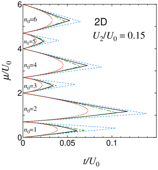
Figure 1: (Color online) Phase diagram obtained by the strong-coupling expansion [Eqs. (13)–(16)] for $U_{2}/U_{0}=0.15$ in 2D. The solid curves show the results up to the third order of $t$. Results up to the first order (second order) of $t$ are also shown by the blue dashed (green dot-dashed) curve. The red dotted curve shows the results obtained by PMFA.

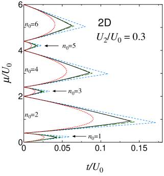
Figure 2: (Color online) Same plot as in Fig. 1 but for $U_{2}/U_{0}=0.3$ in 2D.

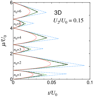
Figure 3: (Color online) Same plot as in Fig. 1 but for $U_{2}/U_{0}=0.15$ in 3D.

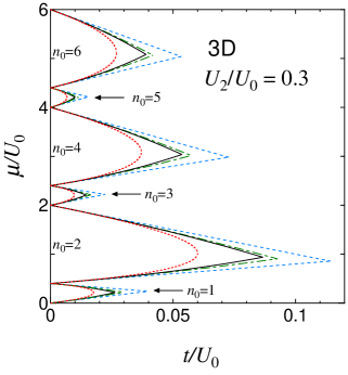
Figure 4: (Color online) Same plot as in Fig. 1 but for $U_{2}/U_{0}=0.3$ in 3D.

III.4 Consistency with PMFA

PMFA involves MF decoupling theory using a perturbative expansion of the SF order parameter. If the SF–MI transition is of the second order, the phase-boundary curve obtained by PMFA is exact in infinite dimensions. Thus, if we expand the equation for this phase-boundary curve, obtained by PMFA up to the third order of $zt$, it must agree with the proposed strong-coupling expansion in infinite dimensions. The results of the expansion of this phase-boundary curve obtained by PMFA [Eqs. (30) and (46) of Ref. Tsuchiya ] are given by Eqs. (17)–(20) of Appendix B. The results are consistent with the proposed strong-coupling expansion. Specifically, we find that the solutions of the equations $E_{\rm MI,even(odd)}(n_{0})=E^{\rm part(hole)}(n_{0})_{\rm def,even(odd)}$ are the same as Eqs. (17)–(20) under the limit $z\rightarrow\infty$ and $t\rightarrow 0$ with constant $zt$.

III.5 Critical value of $t$ at the peak of the Mott lobe

In this section, we examine the critical value $t_{\rm C}$ of the hopping parameter $t$ at the peak of the Mott lobe, where the upper branch of the $t$–$\mu$ curve for the phase-boundary converges with its lower branch. In addition, the dependence of $t_{\rm C}$ on $U_{2}$ indicates the range over which the proposed expansion up to the third order of $t$ may be applied.

Figure 5 shows the dependence of $t_{\rm C}$ on $U_{2}$ for a Mott lobe with an even number of bosons ($n_{0}=2$). The curves in infinite dimensions obtained by PMFA and those obtained by the strong-coupling expansion up to the third order of $t$ (see previous Sec. III D) are smoothly increasing functions of $U_{2}$. When $U_{2}/U_{0}$ is large, the results obtained by the strong-coupling expansion up to the third order of $t$ in 2D and 3D show a similar dependence of $t_{\rm C}$ on $U_{2}$. However, the results show a strange behavior for $U_{2}/U_{0}\sim 0.1$, and the curves stop at small $U_{2}/U_{0}$ because we cannot find $t_{\rm C}$ as the upper and lower branches of the $t$–$\mu$ curve no longer converge. Such a situation also occurs for greater $n$. Because $U_{2}$ stabilizes the MI phase with even boson filling against the SF phase, the results of PMFA and of the strong-coupling expansion in infinite dimensions agree with physical intuition. The small $U_{2}$ regime is hazardous for the strong-coupling expansion in finite dimensions because a few denominators of the expansion contain $3U_{2}$, which corresponds to the spin-excitation energy [$E(S=2)-E(S=0)$] of an intermediate state that appears in perturbative calculation. This problem can be solved only by expanding $\mu$ to infinite orders of $t$. However, the terms involving $3U_{2}$ disappear in the denominators of the strong-coupling expansion in infinite dimensions, so we obtain $t_{\rm C}$ even for small $U_{2}/U_{0}$. On the other hand, the possibility of a first-order transition should not be ignored for a small $U_{2}/U_{0}$ Kimura1 .

Figure 6 shows the same plot as Fig. 5 but for a Mott lobe with an odd number of bosons ($n_{0}=1$). The parameter $t_{\rm C}$ obtained by PMFA is a smoothly decreasing function of $U_{2}$ and goes to zero at $U_{2}/U_{0}=0.5$, where the Mott lobes for odd boson filling disappear. Moreover, the other curves also show that $t_{\rm C}$ is a decreasing function of $U_{2}$ when $U_{2}/U_{0}$ is large. However, $t_{\rm C}$ is a rapidly increasing function of $U_{2}$ for $U_{2}/U_{0}<0.1$ and $t_{\rm C}=0$ at $U_{2}/U_{0}=0$. This is also because, in the strong-coupling expansion up to the third order of $t$, a few denominators contain $3U_{2}$ (here, this is true not only in 2D or 3D but also in infinite dimensions). Therefore, $t_{\rm C}\rightarrow 0$ when $U_{2}/U_{0}\rightarrow 0$, so that the two branches of the $t$–$\mu$ curve converge. For greater $n_{0}$, $t_{\rm C}$ cannot be obtained for a small $U_{2}/U_{0}$ for the same reason as that given in the previous paragraph for the case of even $n_{0}$ (figure not shown). A similar problem can also occur for $U_{2}/U_{0}\approx 0.5$ in 1D because a few terms in the expansion include $U_{0}-2U_{2}$ in their denominator. This problem can also be solved only by expanding $\mu$ to infinite orders of $t$.

In summary, because the parameter $t_{\rm C}$ may be an increasing (decreasing) function of $U_{2}$ for a Mott lobe with even (odd) boson filling, the proposed strong-coupling expansion is reliable for large (intermediate) values of $U_{2}$.

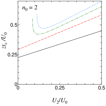
Figure 5: (Color online) Dependence of $t_{\rm C}$ on $U_{2}$ for Mott lobe with even boson filling ($n_{0}=2$). The blue short-dashed, green dot-dashed, and red long-dashed curves show the results obtained by the strong-coupling expansion up to the third order of $t$ in 2D, 3D, and infinite dimensions, respectively. The solid curves show the results obtained by PMFA.

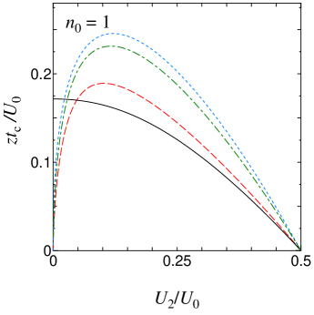
Figure 6: (Color online) Same plot as in Fig. 5 but for Mott lobe with odd boson filling ($n_{0}=1$).

III.6 Extrapolation methods

The expansion up to the third order of $t$ has a few problems. For example, the phase-boundary curve, including the value of $t_{\rm C}$, does not completely converge. From a qualitative point of view, the expansion does not provide an appropriate scaling form of the phase-boundary curve near $t_{\rm C}$. However, in order to improve the phase diagram, we attempt two extrapolation methods in working toward an infinite-order theory in this section.

III.6.1 Linear fit of $t_{\rm C}$

Critical-point extrapolation, which was proposed in Ref. Freericks , is a simple method that involves a least-squares fit to obtain a straight line that best fits the data.

Figure 7 shows the critical point $t_{\rm c}$ at the peak of the Mott lobe for each order $m$ of the strong-coupling expansion. The data for $t_{\rm C}$ lie approximately on a straight line. The data can be extrapolated to the infinite order ($1/m\rightarrow 0$) by least-squares fitting to obtain the straight line that best fits the data. Specifically, extrapolating the straight line to where it intersects the vertical axis gives the infinite-order $t_{\rm C}$.

Table 1 gives the infinite-order fitting data. The fitting error comment1 is very small when $U_{2}/U_{0}$ is large, where strong-coupling expansion can be more reliable compared to the small-$U_{2}/U_{0}$ regime (which is consistent with the dependence of $t_{\rm C}$ on $U_{2}$ discussed in Sec. III E).

Figure 7: Solid circles show $t_{\rm C}$ obtained by the proposed strong-coupling expansion up to the first, second, and third order of $t$ for $U_{2}/U_{0}=0.3$ in 2D and 3D. The data are labeled for $n_{0}=1$ Mott lobes and $n_{0}=2$ Mott lobes. The horizontal axis is the inverse of the order of expansion ($1/{\rm order}=1/3,1/2,1$ for third, second, and first orders, respectively). The dashed lines are least-square linear fits of the solid circles.

III.6.2 Extrapolation of phase-boundary curves

The proposed phase-boundary curve obtained by expansion up to the third order of $t$ has a cusp at the peak of the Mott lobe. However, it can be assumed that the chemical potential has the following power-law scaling near $t_{\rm C}$, similar to that of the spinless BH model in 2D or 3D:

$$\mu=A(t)\pm B(t)(t_{\rm C}-t)^{z\nu}.$$ (10)

The following fitting method is called chemical-potential fitting Freericks ; Iskin . Here $A(t)\approx a+bt+ct^{2}+dt^{3}$ and $B(t)\approx\alpha+\beta t+\gamma t^{2}+\delta t^{3}$ are the regular functions of $t$. The parameter $z\nu$ is the critical exponent in the model. By using expansion up to the third order of $t$, we immediately determine $a$, $b$, $c$, and $d$ by setting $A(t)=[\mu^{\rm part}(t)+\mu^{\rm hole}(t)]/2$. In addition, by assuming that the scaling is the same as that of the spinless BH model Fisher ; Freericks , we set $z\nu\simeq 2/3$ for $d=2$ and $z\nu=1/2$ for $d>2$ in the $d$-dimensional spin-1 BH model comment2 . By setting $\delta=0$, we obtain $\alpha$, $\beta$, $\gamma$, and $t_{\rm C}$ by comparing the Taylor expansion of $t$ in $B(t)(t_{\rm C}-t)^{z\nu}$ with $[\mu^{\rm part}(t)-\mu^{\rm hole}(t)]/2$. The results for $t_{\rm C}$ are given in Table 1, and the phase-boundary curves obtained by the above fitting are shown in Fig. 8 for 2D and in Fig. 9 for 3D.

By combining these two fitting methods, we obtain the phase-boundary curve. Specifically, we use the value of $t_{\rm C}$ obtained by the least-squares fit to compare $B(t)(t_{\rm C}-t)^{z\nu}$ with $[\mu^{\rm part}(t)-\mu^{\rm hole}(t)]/2$. Here we include the $\delta t^{3}$ term in $B(t)$. The obtained phase-boundary curves are also plotted in Figs. 8 and 9. The phase-boundary curves obtained by these two fitting methods are very similar, especially in 2D. The phase-boundary curves obtained by these two fitting methods are more similar to those obtained by PMFA in 3D than to those obtained in 2D, as expected.

Table 1: List of critical points $t_{c}/U_{0}$.

		Two dimensions			Three dimensions
$n_{0}$	$U_{2}/U_{0}$	$(t_{c}/U_{0})_{\rm 3rd}$	$t_{c}/U_{0}$	$t_{c}/U_{0}$	$(t_{c}/U_{0})_{\rm 3rd}{}^{\rm a}$	$t_{c}/U_{0}{}^{\rm b}$	$t_{c}/U_{0}{}^{\rm c}$
1	0.2	0.0568	0.0400 $\pm$ 0.0010	0.0482	0.0353	0.0224 $\pm$ 0.0020	0.0269
	0.3	0.0429	0.0349 $\pm$ 0.0021	0.0365	0.0263	0.0195 $\pm$ 0.0001	0.0202
	0.4	0.0234	0.0205 $\pm$ 0.0015	0.0201	0.0143	0.0115 $\pm$ 0.0004	0.0110
2	0.2	0.1221	0.1019 $\pm$ 0.0218	0.1084	0.0758	0.0615 $\pm$ 0.0078	0.0607
	0.3	0.1388	0.1205 $\pm$ 0.0068	0.1208	0.0866	0.0722 $\pm$ 0.0021	0.0683
	0.4	0.1567	0.1389 $\pm$ 0.0010	0.1356	0.0978	0.0827 $\pm$ 0.0009	0.0766
3	0.2	0.0313	0.0216 $\pm$ 0.0014	0.0266	0.0195	0.0121 $\pm$ 0.0016	0.0149
	0.3	0.0236	0.0190 $\pm$ 0.0009	0.0201	0.0145	0.0106 $\pm$ 0.0001	0.0111
	0.4	0.0129	0.0113 $\pm$ 0.0008	0.0111	0.0079	0.0063 $\pm$ 0.0002	0.0061
4	0.2	0.0754	0.0611 $\pm$ 0.0150	0.0669	0.0469	0.0368 $\pm$ 0.0057	0.0375
	0.3	0.0859	0.0726 $\pm$ 0.0057	0.0747	0.0536	0.0435 $\pm$ 0.0021	0.0422
	0.4	0.0971	0.0840 $\pm$ 0.0007	0.0839	0.0606	0.0498 $\pm$ 0.0003	0.0474

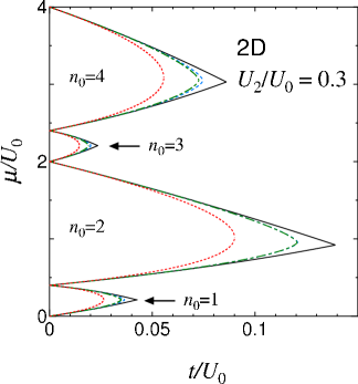
Figure 8: (Color on line) Phase diagram obtained by strong-coupling expansion up to the third order of $t$ (solid curve) for $U_{2}/U_{0}=0.3$ in 2D and its extrapolation to the infinite order of $t$. The blue dashed (green dot-dashed) curve shows the chemical-potential fitting without (with) the least-squares fit for $t_{\rm C}$. The blue dashed and green dot-dashed curves are similar to each other. In particular, the two curves for the $n_{0}=2$ Mott lobe are indistinguishable. The red dotted curve shows the PMFA results. The smallest area Mott lobe is obtained by PMFA.

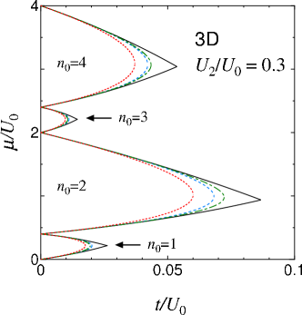
Figure 9: Same plot as that in Fig. 8 for 3D.

III.7 One dimension

In 1D, the MI phase exhibits a very rich spin structure; however, the strong-coupling expansion is based on the spin-singlet (spin-nematic) states for even (odd) boson filling. In particular, for odd boson filling, the ground state may be the spin-dimerized state over a wide parameter space. Thus, the results obtained by the proposed strong-coupling expansion cannot be directly applied to 1D especially for odd boson fillings. The range of $U_{2}/U_{0}$, in which we can obtain $t_{\rm C}$ at the peak of the Mott lobe, is more limited compared to that in 2D or 3D. For instance, $U_{2}/U_{0}\geq 0.255$ is required to obtain $t_{\rm C}$ for the $n_{0}=2$ Mott lobe.

Nevertheless, we briefly examine the phase diagram because, to date, most numerical simulations are for 1D. Figures 10 and 11 show the phase diagrams obtained by the proposed strong-coupling expansion up to the third order of $t$ for $U_{2}/U_{0}=0.3$ and $U_{2}/U_{0}=0.4$, respectively. In Fig. 11, the upper and lower branches of the $n_{0}=1$ Mott lobe do not converge, which precludes a closed phase-boundary curve. Figures 10 and 11 also show that the strong-coupling expansion converges when it goes from the first to third order of $t$, although the convergence is not excellent compared with that in 2D or 3D (Figs. 1–4).

For $U_{2}/U_{0}=0.3$, agreement with the phase diagram obtained with DMRG Rizzi is not excellent but satisfactory for the Mott lobe with even boson fillings. For example, with the strong-coupling expansion, $t_{\rm C}/U_{0}=0.327$, and with DMRG, $t_{\rm C}/U_{0}\simeq 0.47$ (as per our interpretation of Fig. 1 in Ref. Rizzi ). However, for $U_{2}/U_{0}=0.4$, the results do not agree with the QMC results shown in Fig. 1 of Ref. Apaja : $t_{\rm C}/U_{0}=0.422$ using the proposed strong-coupling expansion and $t_{\rm C}/U_{0}\simeq 0.7$ from the QMC results. In general, larger $t$ is required to obtain the SF phase for large $U_{0}$ and/or $U_{2}$, where the higher-order terms of $t$ become more prominent. Therefore, we may have to expand up to fourth or even higher order in order to reduce the discrepancy. Otherwise, we may have to assume another MI phase such as a nematic MI phase for even boson filling.

Figures 10 and 11 also show the results obtained by PMFA, which may be inaccurate in 1D. We find a very large difference between these results and those of the strong-coupling expansion.

As mentioned in Sec. III F, we also attempt to extrapolate the results to infinite order in $t$. In the least-squares fit in $t_{\rm C}$, we cannot improve the results as extensively; for instance, $t_{\rm C}/U_{0}=0.433\pm 0.030$ for $U_{2}/U_{0}=0.4$ for the $n_{0}=2$ Mott lobe. We attempt the fit with the chemical potential by assuming the Kosterlitz–Thouless form, as per Ref. Freericks , although the fit is not successful (figure not shown).

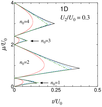
Figure 10: (Color online) 1D phase diagram at $U_{2}/U_{0}=0.3$. The solid curves show the results obtained by strong-coupling expansion up to the third order of $t$. Results up to the first order (second order) of $t$ are also shown by the blue dashed (green dot-dashed) curve. The red dotted curve shows the results obtained by PMFA.

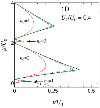
Figure 11: (Color online) Similar plot to Fig. 10 for $U_{2}/U_{0}=0.4$ in 1D, except for the dashed curves for the $n_{0}=1$ Mott lobe. For $n_{0}=1$, the upper and lower branches of the Mott lobe do not converge at third order in $t$, so a closed phase-boundary curve is not obtained.

III.8 Summary and Discussion

In this study, we used a strong-coupling expansion of the hopping parameter $t$ to obtain analytical results for the phase diagram. In the limit of infinite dimensions, the $t$–$\mu$ phase-boundary curves were consistent with the exact results obtained by PMFA.

Overall, the convergence of the phase-boundary curves from the first to the third order was excellent. The dependence of $t_{\rm C}$ on $U_{2}$ at the peak of the Mott lobe with even (odd) boson filling indicated a reliable strong-coupling expansion at large (intermediate) values of $U_{2}$.

We attempted to extrapolate the results to the infinite order in $t$ by a least-squares fit and a chemical-potential fit to $t_{\rm C}$. The linear fitting error of $t_{\rm C}$ was very small for large $U_{2}$. As expected, the fitting results of the phase-boundary curves agreed better with those of PMFA in 3D than with those in 2D. We also compared the 1D phase-boundary curves obtained by the strong-coupling expansion with those obtained by numerical simulations. For $U_{2}/U_{0}=0.3$, satisfactory (but not excellent) agreement was achieved between the 1D phase-boundary curves and those obtained by DMRG.

The proposed strong-coupling expansion depends on the $t=0$ ground state. However, the MI phase can be more complicated. We must consider the dimerized-spin phase for odd boson filling, which can be the ground state in 1D. In addition, we should consider the nematic spin phase for even boson filling, which can be the ground state for weak $U_{2}$. To analytically determine the complete phase diagram, these spin phases must be included in the strong-coupling expansion. The possible first-order transition should also be studied on an equal footing with the second-order transition. These remain problems for future work.

Appendix A Energies of Mott insulator and defect states determined by strong-coupling expansion

By using $\Psi_{\rm even}$ and $\Psi_{\rm odd}$ [Eqs. (4) and (5)], the energies of the MI state per site are

$$\frac{E_{\rm MI,even}(n_{0})}{N} = \frac{U_{0}}{2}n_{0}(n_{0}-1)-U_{2}n_{0}-n_{0}\mu-\frac{zt^{2}}{3}\frac{n_{0}(n_{0}+3)}{U_{0}+2U_{2}},$$ (11)

$$\frac{E_{\rm MI,odd}(n_{0})}{N} = \frac{U_{0}}{2}n_{0}(n_{0}-1)-U_{2}(n_{0}-1)-n_{0}\mu$$ (12)

$$-zt^{2}\Big{[}\frac{34}{225}\frac{(n_{0}+4)(n_{0}-1)}{U_{0}+4U_{2}}+\frac{4}{45}\frac{2n_{0}^{2}+6n_{0}+7}{U_{0}+U_{2}}+\frac{1}{9}\frac{(n_{0}+1)(n_{0}+2)}{U_{0}-2U_{2}}\Big{]}\ \$$

up to third order in $t$. On the other hand, by using $\Psi^{\rm part}_{\rm even}$, $\Psi^{\rm hole}_{\rm even}$, $\Psi^{\rm part}_{\rm odd}$, and $\Psi^{\rm hole}_{\rm odd}$ [Eqs. (6)–(9)], the energies of the defect states are

$$E^{\rm part}_{\rm def,even}(n_{0})-E_{\rm MI,even}(n_{0})$$ (13)

$$= U_{0}n-\mu-zt\frac{n_{0}+3}{3}$$

$$-\frac{z(z-7)t^{2}}{9}\frac{n_{0}(n_{0}+3)}{U_{0}+2U_{2}}-\frac{zt^{2}n_{0}}{9}\Big{[}2\Big{(}\frac{n_{0}+5}{2U_{0}+3U_{2}}+\frac{n_{0}+3}{3U_{2}}\Big{)}+\frac{n_{0}+2}{2U_{0}}\Big{]}$$

$$-\frac{zt^{3}}{27}n_{0}(n_{0}+3)\Big{\{}(z-1)\Big{[}\frac{(2n_{0}+3)z-3(3n_{0}+8)}{(U_{0}+2U_{2})^{2}}$$

$$+\frac{2}{U_{0}+2U_{2}}\Big{(}2\frac{n_{0}+5}{2U_{0}+3U_{2}}+\frac{n_{0}+2}{2U_{0}}\Big{)}+\frac{4(n_{0}+3)}{3U_{2}(U_{0}+2U_{2})}\Big{]}$$

$$-z\Big{[}2\Big{(}\frac{n_{0}+5}{(2U_{0}+3U_{2})^{2}}+\frac{n_{0}+3}{(3U_{2})^{2}}\Big{)}+\frac{n_{0}+2}{(2U_{0})^{2}}\Big{]}+\frac{4}{3U_{2}}\Big{(}\frac{1}{5}\frac{n_{0}+5}{2U_{0}+3U_{2}}+\frac{n_{0}+2}{2U_{0}}\Big{)}\Big{\}},$$

$$E^{\rm hole}_{\rm def,even}(n_{0})-E_{\rm MI,even}(n_{0})$$ (14)

$$= -U_{0}(n_{0}-1)+2U_{2}+\mu-zt\frac{n_{0}}{3}$$

$$-\frac{z(z-7)t^{2}}{9}\frac{n_{0}(n_{0}+3)}{U_{0}+2U_{2}}-\frac{zt^{2}(n_{0}+3)}{9}\Big{[}2\Big{(}\frac{n_{0}-2}{2U_{0}+3U_{2}}+\frac{n_{0}}{3U_{2}}\Big{)}+\frac{n_{0}+1}{2U_{0}}\Big{]}$$

$$-\frac{zt^{3}}{27}n_{0}(n_{0}+3)\Big{\{}(z-1)\Big{[}\frac{(2n_{0}+3)z-3(3n_{0}+1)}{(U_{0}+2U_{2})^{2}}$$

$$+\frac{2}{U_{0}+2U_{2}}\Big{(}2\frac{n_{0}-2}{2U_{0}+3U_{2}}+\frac{n_{0}+1}{2U_{0}}\Big{)}+\frac{4n_{0}}{3U_{2}(U_{0}+2U_{2})}\Big{]}$$

$$-z\Big{[}2\Big{(}\frac{n_{0}-2}{(2U_{0}+3U_{2})^{2}}+\frac{n_{0}}{(3U_{2})^{2}}\Big{)}+\frac{n_{0}+1}{(2U_{0})^{2}}\Big{]}+\frac{4}{3U_{2}}\Big{(}\frac{1}{5}\frac{n_{0}-2}{2U_{0}+3U_{2}}+\frac{n_{0}+1}{2U_{0}}\Big{)}\Big{\}},$$

$$E^{\rm part}_{\rm def,odd}(n_{0})-E_{\rm MI,odd}(n_{0})$$ (15)

$$= U_{0}n_{0}-2U_{2}-zt\frac{n_{0}+1}{3}-\mu$$

$$-\frac{z(z-3)t^{2}}{9}(n_{0}+1)\Big{[}\frac{n_{0}+2}{U_{0}-2U_{2}}+\frac{4}{5}\frac{n_{0}-1}{U_{0}+U_{2}}\Big{]}$$

$$-\frac{zt^{2}}{9}(n_{0}+4)\Big{[}2\frac{n_{0}-1}{2U_{0}+3U_{2}}+\frac{n_{0}+2}{2U_{0}}-\frac{68}{25}\frac{n_{0}-1}{U_{0}+4U_{2}}-\frac{8}{5}\frac{n_{0}+2}{U_{0}+U_{2}}\Big{]}$$

$$-\frac{2}{45}z(2z+3)t^{2}\frac{(n_{0}+1)(n_{0}+4)}{3U_{2}}$$

$$-\frac{z(z-1)t^{3}}{27}\frac{(n_{0}+1)(n_{0}+2)}{(U_{0}-2U_{2})^{2}}\big{[}(2n_{0}+3)z-(5n_{0}+6)\big{]}$$

$$-\frac{4}{675}z(z-1)t^{3}\frac{n_{0}+1}{(U_{0}+U_{2})^{2}}\big{[}(n_{0}-1)(9n_{0}+1)z-2(17n_{0}^{2}+26n_{0}+32)\big{]}$$

$$-\frac{z(z-1)^{2}t^{3}}{27}\frac{n_{0}+1}{U_{0}+U_{2}}\Big{[}\frac{32}{25}\frac{(n_{0}-1)(n_{0}+4)}{U_{0}+4U_{2}}+\frac{8}{5}\frac{(n_{0}+2)(2n_{0}+3)}{U_{0}-2U_{2}}\Big{]}$$

$$-\frac{2}{27}z(z-1)t^{3}(n_{0}+1)(n_{0}+4)\Big{\{}\frac{n_{0}-1}{2U_{0}+3U_{2}}\Big{[}\frac{34}{25}\frac{1}{U_{0}+4U_{2}}+\frac{4}{5}\frac{1}{U_{0}+U_{2}}\Big{]}$$

$$+\frac{n_{0}+2}{2U_{0}}\Big{[}\frac{1}{U_{0}-2U_{2}}+\frac{4}{5}\frac{1}{U_{0}+U_{2}}\Big{]}+\frac{1}{3U_{2}}\Big{[}\frac{2}{25}(8z+9)\frac{n_{0}-1}{U_{0}+4U_{2}}+\frac{4}{5}z\frac{n_{0}+2}{U_{0}+U_{2}}\Big{]}\Big{\}}$$

$$-\frac{4}{135}z(2z+3)t^{3}\frac{(n_{0}+1)(n_{0}+4)}{3U_{2}}\Big{[}\frac{1}{5}\frac{n_{0}-1}{2U_{0}+3U_{2}}+\frac{n_{0}+2}{2U_{0}}\Big{]}$$

$$+\frac{2}{675}zt^{3}\frac{(n_{0}+1)(n_{0}+4)}{(3U_{2})^{2}}\big{[}2(n_{0}-11)z^{2}+9(3n_{0}+7)z-9(n_{0}+4)\big{]}$$

$$+\frac{zt^{3}}{27}(n_{0}+1)(n_{0}+4)\Big{[}\frac{68}{25}(z-1)\frac{n_{0}-1}{(U_{0}+4U_{2})^{2}}+2z\frac{n_{0}-1}{(2U_{0}+3U_{2})^{2}}+z\frac{n_{0}+2}{(2U_{0})^{2}}\Big{]},$$

$$E^{\rm hole}_{\rm def,odd}(n_{0})-E_{\rm MI,odd}(n_{0})$$ (16)

$$= -U_{0}(n_{0}-1)-zt\frac{n_{0}+2}{3}+\mu$$

$$-\frac{z(z-3)t^{2}}{9}(n_{0}+2)\Big{[}\frac{n_{0}+1}{U_{0}-2U_{2}}+\frac{4}{5}\frac{n_{0}+4}{U_{0}+U_{2}}\Big{]}$$

$$-\frac{zt^{2}}{9}(n_{0}-1)\Big{[}2\frac{n_{0}+4}{2U_{0}+3U_{2}}+\frac{n_{0}+1}{2U_{0}}-\frac{68}{25}\frac{n_{0}+4}{U_{0}+4U_{2}}-\frac{8}{5}\frac{n_{0}+1}{U_{0}+U_{2}}\Big{]}$$

$$-\frac{2}{45}z(2z+3)t^{2}\frac{(n_{0}-1)(n_{0}+2)}{3U_{2}}$$

$$-\frac{z(z-1)t^{3}}{27}\frac{(n_{0}+1)(n_{0}+2)}{(U_{0}-2U_{2})^{2}}\big{[}(2n_{0}+3)z-(5n_{0}+9)\big{]}$$

$$-\frac{4}{675}z(z-1)t^{3}\frac{n_{0}+2}{(U_{0}+U_{2})^{2}}\big{[}(n_{0}+4)(9n_{0}+26)z-2(17n_{0}^{2}+76n_{0}+107)\big{]}$$

$$-\frac{z(z-1)^{2}t^{3}}{27}\frac{n_{0}+2}{U_{0}+U_{2}}\Big{[}\frac{32}{25}\frac{(n_{0}-1)(n_{0}+4)}{U_{0}+4U_{2}}+\frac{8}{5}\frac{(n_{0}+1)(2n_{0}+3)}{U_{0}-2U_{2}}\Big{]}$$

$$-\frac{2}{27}z(z-1)t^{3}(n_{0}-1)(n_{0}+2)\Big{\{}\frac{n_{0}+4}{2U_{0}+3U_{2}}\Big{[}\frac{34}{25}\frac{1}{U_{0}+4U_{2}}+\frac{4}{5}\frac{1}{U_{0}+U_{2}}\Big{]}$$

$$+\frac{n_{0}+1}{2U_{0}}\Big{[}\frac{1}{U_{0}-2U_{2}}+\frac{4}{5}\frac{1}{U_{0}+U_{2}}\Big{]}+\frac{1}{3U_{2}}\Big{[}\frac{2}{25}(8z+9)\frac{n_{0}+4}{U_{0}+4U_{2}}+\frac{4}{5}z\frac{n_{0}+1}{U_{0}+U_{2}}\Big{]}\Big{\}}$$

$$-\frac{4}{135}z(2z+3)t^{3}\frac{(n_{0}-1)(n_{0}+2)}{3U_{2}}\Big{[}\frac{1}{5}\frac{n_{0}+4}{2U_{0}+3U_{2}}+\frac{n_{0}+1}{2U_{0}}\Big{]}$$

$$+\frac{2}{675}zt^{3}\frac{(n_{0}-1)(n_{0}+2)}{(3U_{2})^{2}}\big{[}2(n_{0}+14)z^{2}+9(3n_{0}+2)z-9(n_{0}-1)\big{]}$$

$$+\frac{zt^{3}}{27}(n_{0}-1)(n_{0}+2)\Big{[}\frac{68}{25}(z-1)\frac{n_{0}+4}{(U_{0}+4U_{2})^{2}}+2z\frac{n_{0}+4}{(2U_{0}+3U_{2})^{2}}+z\frac{n_{0}+1}{(2U_{0})^{2}}\Big{]}$$

up to third order in $t$. By equating the right-hand side of Eqs. (13)–(16) with zero, we obtain the SF–MI phase-boundary curve.

Appendix B Expansion of phase-boundary curve obtained by PMFA

The phase-boundary curves obtained by PMFA are given by Eqs. (30) and (46) of Ref. Tsuchiya for even and odd MI lobes, respectively. We can straightforwardly expand the results up to third order in $zt$ for even MI lobes:

$$\mu^{\rm part}_{\rm even} = U_{0}n_{0}-\frac{n_{0}+3}{3}zt-\frac{n_{0}(n_{0}+3)}{9}\frac{(zt)^{2}}{U_{0}+2U_{2}}$$ (17)

$$-\frac{n_{0}(n_{0}+3)(2n_{0}+3)}{27}\frac{(zt)^{3}}{(U_{0}+2U_{2})^{2}}$$

$$\mu^{\rm hole}_{\rm even} = U_{0}(n_{0}-1)-2U_{2}+\frac{n_{0}}{3}zt+\frac{n_{0}(n_{0}+3)}{9}\frac{(zt)^{2}}{U_{0}+2U_{2}}$$ (18)

$$+\frac{n_{0}(n_{0}+3)(2n_{0}+3)}{27}\frac{(zt)^{3}}{(U_{0}+2U_{2})^{2}}$$

and for odd MI lobes,

$$\mu^{\rm part}_{\rm odd} = U_{0}n_{0}-2U_{2}-\frac{n_{0}+3}{3}zt-\frac{n_{0}+1}{9}\Big{[}\frac{n_{0}+2}{U_{0}-2U_{2}}+\frac{4}{5}\Big{(}\frac{n_{0}-1}{U_{0}+U_{2}}+\frac{n_{0}+4}{3U_{2}}\Big{)}\Big{]}(zt)^{2}$$ (19)

$$-\frac{n_{0}+1}{27}\Big{\{}\frac{(n_{0}+2)(2n_{0}+3)}{(U_{0}-2U_{2})^{2}}+\frac{4}{25}\frac{(n_{0}-1)(9n_{0}+1)}{(U_{0}+U_{2})^{2}}-\frac{4}{25}\frac{(n_{0}+4)(n_{0}-11)}{(3U_{2})^{2}}$$

$$+\frac{24}{25}\frac{(n_{0}+4)(3n_{0}+2)}{3U_{2}(U_{0}+U_{2})}+\frac{8}{5}\frac{(n_{0}+2)(2n_{0}+3)}{(U_{0}+U_{2})(U_{0}-2U_{2})}\Big{\}}(zt)^{3}$$

$$\mu^{\rm hole}_{\rm odd} = U_{0}(n_{0}-1)+\frac{n_{0}+2}{3}zt+\frac{n_{0}+2}{9}\Big{[}\frac{n_{0}+1}{U_{0}-2U_{2}}+\frac{4}{5}\Big{(}\frac{n_{0}-1}{3U_{2}}+\frac{n_{0}+4}{U_{0}+U_{2}}\Big{)}\Big{]}(zt)^{2}$$ (20)

$$+\frac{n_{0}+2}{27}\Big{\{}\frac{(n_{0}+1)(2n_{0}+3)}{(U_{0}-2U_{2})^{2}}+\frac{4}{25}\frac{(n_{0}+4)(9n_{0}+26)}{(U_{0}+U_{2})^{2}}-\frac{4}{25}\frac{(n_{0}-1)(n_{0}+14)}{(3U_{2})^{2}}$$

$$+\frac{24}{25}\frac{(n_{0}-1)(3n_{0}+7)}{3U_{2}(U_{0}+U_{2})}+\frac{8}{5}\frac{(n_{0}+1)(2n_{0}+3)}{(U_{0}+U_{2})(U_{0}-2U_{2})}\Big{\}}(zt)^{3}.$$

References

- (1) D. M. Stamper-Kurn, M. R. Andrews, A. P. Chikkatur, S. Inouye, H.-J. Miesner, J. Stenger, and W. Ketterle, Phys. Rev. Lett. 80, 2027 (1998).
- (2) For reviews, see D. M. Stamper-Kurn and M. Ueda, arXiv:1205.1888.
- (3) M. Greiner, O. Mandel, T. Esslinger, T. W. Hänsch, and I. Bloch, Nature (London) 415, 39 (2002).
- (4) W. S. Bakr, A. Peng, M. E. Tai, R. Ma, J. Simon, J. Gillen, S. Foelling, L. Pollet, and M. Greiner, Science 329, 547 (2010).
- (5) W. S. Bakr, J. I. Gillen, A. Peng, S. Foelling, and M. Greiner, Nature (London) 462, 74 (2009).
- (6) M. M. Endres, M. Cheneau, T. Fukuhara, C. Weitenberg, P. Schauß, C. Gross, L. Mazza, M.C. Banuls, L. Pollet, I. Bloch, and S. Kuhr, Science 334, 200 (2011).
- (7) C. Weitenberg, M. Endres, J. F. Sherson, M. Cheneau, P. Schauß, T. Fukuhara, I. Bloch, and S. Kuhr, Nature (London) 471, 319 (2011).
- (8) D. Jaksch, C. Bruder, J. I. Cirac, C. W. Gardiner, and P. Zoller, Phys. Rev. Lett. 81, 3108 (1998).
- (9) M.P.A. Fisher, P.B. Weichman, G. Grinstein, and D.S. Fisher, Phys. Rev. B 40, 546 (1989).
- (10) E. Demler and F. Zhou, Phys. Rev. Lett. 88, 163001 (2002).
- (11) S.K. Yip, Phys. Rev. Lett. 90, 250402 (2003).
- (12) A. Imambekov, M. Lukin, and E. Demler, Phys. Rev. A 68, 063602 (2003).
- (13) M. Snoek and F. Zhou, Phys. Rev. B 69, 094410 (2004).
- (14) F. Zhou and M. Snoek, Ann. Phys. (NY) 308, 692 (2003); F. Zhou, Europhys. Lett. 63, 505 (2003).
- (15) N. Uesugi and M. Wadati, J. Phys. Soc. Jpn. 72, 1041 (2003).
- (16) S. Tsuchiya, S. Kurihara, and T. Kimura, Phys. Rev. A 70, 043628 (2004).
- (17) T. Kimura, S. Tsuchiya, and S. Kurihara, Phys. Rev. Lett. 94, 110403 (2005).
- (18) K. V. Krutitsky and R. Graham, Phys. Rev. A 70, 063610 (2004).
- (19) K.V. Krutitsky, M. Timmer, and R. Graham, Phys. Rev. A 71, 033623 (2005).
- (20) T. Kimura, S. Tsuchiya, M. Yamashita, and S. Kurihara, J. Phys. Soc. Jpn. 75, 074601 (2006).
- (21) M. Yamashita and M. W. Jack, Phys. Rev. A 76, 023606 (2007).
- (22) M. Rizzi, D. Rossini, G. De Chiara, S. Montangero, and R. Fazio, Phys. Rev. Lett. 95, 240404 (2005).
- (23) S. Bergkvist, I. P. McCulloch, and A. Rosengren, Phys. Rev. A 74, 053419 (2006).
- (24) G. G. Batrouni, V. G. Rousseau, and R. T. Scalettar, Phys. Rev. Lett. 102, 140402 (2009).
- (25) V. Apaja and O. F. Syljuåsen, Phys. Rev. A 74, 035601 (2006).
- (26) Y. Toga, H. Tsuchiura, M. Yamashita, K. Inaba, and H. Yokoyama, J. Phys. Soc. Jpn. 81, 063001 (2012).
- (27) M. Łącki, S. Paganelli, V. Ahufinger, A. Sanpera, and J. Zakrzewski, Phys. Rev. A 83, 013605 (2011).
- (28) A. Wagner, A. Nunnenkamp, and C. Bruder, Phys. Rev. A 86, 023624 (2012).
- (29) D. van Oosten, P. van der Straten, and H.T.C. Stoof, Phys. Rev. A 63, 053601 (2001).
- (30) For instance, by a similar calculation to that of Ref. Kimura1 , we obtain that the first-order SF–MI transition from the Mott lobe with two bosons per site disappears when in the Gutzwiller MF study.
- (31) J. K. Freericks and H. Monien, Phys. Rev. B 53, 2691 (1996); J. K. Freericks and H. Monien, Europhys. Lett. 26, 545 (1994).
- (32) See, e.g., C. Cohen-Tannoudji, B. Diu, and F. Laloe, Quantum Mechanics (Wiley-Interscience, New York, 1992).
- (33) T. D. Kühner and H. Monien, Phys. Rev. B 58, 14741(R) (1998).
- (34) P. Buonsante,V. Penna, and A.Vezzani,Phys. Rev. B 70, 184520 (2004).
- (35) K. Sengupta and N. Dupuis, Phys. Rev. A 71, 033629 (2005).
- (36) J. K. Freericks, H. R. Krishnamurthy, Y. Kato, N. Kawashima, and N. Trivedi, Phys. Rev. A 79, 053631 (2009).
- (37) V. K. Varma and H. Monien, Phys. Rev. B 84, 195131 (2011).
- (38) M. Iskin and J. K. Freericks, Phys. Rev. A 79, 053634 (2009).
- (39) I. Hen, M. Iskin, and M. Rigol, Phys. Rev. B 81, 064503 (2010).
- (40) M. Iskin, Phys. Rev. A 82, 033630 (2010).
- (41) Here, we adopt a standard deviation twice as large as the error bar because we can use only three data points to form a straight line; thus, the accuracy of the standard deviation is almost the same as the standard deviation. See, e.g., Sec. 2.5 of N. C. Barford, Experimental Measurements: Precision, Error, and Truth, 2nd ed. (Wiley, New York, 1985).
- (42) The critical exponent is determined by phase fluctuation on the fixed-density contour, so we consider that the only relevant degree of freedom is the SF phase, as for the spinless BH model. In addition, at , the critical exponent must be the same as that of the spinless BH model because the spin magnetic quantum number of all bosons must be the same ( are degenerate) in order to maximize the absolute value of kinetic energy, and the spin degree of freedom does not influence the critical behavior. Even if becomes finite (but sufficiently small) and the degeneracy is lifted, the polar state consisting of only bosons (without ) remains the ground state. The critical behavior usually does not depend on the value of microscopic parameters, so the critical behavior for large is probably the same as that for .