The influence of noise sources on cross-correlation amplitudes

We use analytical examples and asymptotic forms to examine the mathematical structure and physical meaning of the seismic cross correlation measurement. We show that in general, cross correlations are not Green’s functions of medium, and may be very different depending on the source distribution. The modeling of noise sources using spatial distributions as opposed to discrete collections of sources is emphasized. When stations are illuminated by spatially complex source distributions, cross correlations show arrivals at a variety of time lags, from zero to the maximum surface-wave arrival time. Here, we demonstrate the possibility of inverting for the source distribution using the energy of the full cross-correlation waveform. The interplay between the source distribution and wave attenuation in determining the functional dependence of cross correlation energies on station-pair distance is quantified. Without question, energies contain information about wave attenuation. However, the accurate interpretation of such measurements is tightly connected to the knowledge of the source distribution.

1 Introduction

Terrestrial seismic noise is generated at a range of temporal frequencies, by human activity, storms, oceanic wave microseisms (e.g., Longuet-Higgins, 1950; Kedar & Webb, 2005; Stehly et al., 2006) and the ocean-excited low-frequency hum of Earth (e.g., Nawa et al., 1998; Rhie & Romanowicz, 2004). Seismic noise is as used as a compelling alternative to earthquake tomography to image the crust. Most importantly, it enables the study of temporal variations of the crust (e.g., Wegler & Sens-Schonfelder, 2007; Brenguier et al., 2008; Zaccarelli et al., 2011; Rivet et al., 2011) and volcanoes (e.g., Brenguier et al., 2007). The cross correlation measurement has a physical flavor that is intrinsically different from the classical tomographic analog, i.e., wavefield displacement. In particular, the time variable in classical tomography is the propagation delay between the source and the station whereas the time lag in cross correlation tomography is connected to the path difference between the source and the two stations.

Under controlled circumstances, such as a when the source distribution is uniform, representation theorems (e.g., Fleury et al., 2010) allow for the cross correlation to be written as a modulation of Green’s function between the stations. In other words, such theorems state that an equally weighted sum over Green’s functions between every source (over all space; constant amplitude) and the stations is equivalent to Green’s function between the stations. However, Earth noise is typically anisotropic and in such a scenario, Green’s functions along some source-station paths are weighted more strongly than others and the elegant correspondence may be lost. Further, the climate is in continuous flux, and the manner of excitation of seismic noise by, e.g., ocean waves, changes through the year (e.g., Stehly et al., 2006). Seismology is a precision science and consequently, modeling the source distribution and its effect on the cross correlation is critical.

The study of terrestrial seismic noise has strong connections with the seismic wavefields of stars, and in particular, the Sun. The use of cross correlations of the wavefield of the Sun to probe interior solar structure was pioneered by Duvall et al. (1993) in a landmark paper. The formal interpretation of these measurements had to wait till the advance by Woodard (1997), who laid the theory of cross correlation on a formal statistical foundation. A number of years later, Gizon & Birch (2002), based on this work, were able to compute kernels for cross correlations of helioseismic noise arising from a distribution of sources. However, Gizon & Birch (2002) did not account for 3-D heterogeneous backgrounds and the rewriting of their formalism in the language of adjoint methods was led by Tromp et al. (2010) for the terrestrial case and by Hanasoge et al. (2011) for the helioseismic scenario. One useful concept that emerged from these articles is that of dealing with source distributions as opposed to a discrete number of them (e.g., Larose et al., 2006; Tsai, 2009). More importantly, the results of Tromp et al. (2010) enabled the computational prediction (in a forward sense) of cross correlations based on a given Earth model and source distribution (this problem has received considerable attention: e.g., Pedersen et al., 2007; Chevrot et al., 2007; Yang & Ritzwoller, 2008; Weaver et al., 2009; Cupillard & Capdeville, 2010; Tsai, 2010; Froment et al., 2010).

In this article, we discuss some of the concepts underlying the cross correlation measurement using a simple 2-D example. Section 2 deals with the cross correlation and its connection to the source distribution. Storms, which excite seismic waves, but sometimes physically move substantial distances over a span of days (i.e., over the measurement window), can be modeled as well, albeit through a more complex ansatz for the distribution. We also introduce the basic partial differential equation governing the wavefield and Green’s function for the simple case studied here. The analysis of the variations of the cross correlation due to the changes in the source distribution, thereby leading to the sensitivity kernel are discussed in Section 3. In particular, its asymptotic form reveals the structure of the source-amplitude kernel. The cross-correlation energy misfit and its kernel are discussed and computed semi-analytically in Section 3.1. Based on this formalism, the impact of non-uniform source distributions on cross correlations is examined and we make a case for imaging of the source distribution and briefly discuss the limitations in Section 3.2.

The operator formulation of the adjoint method discussed by, e.g., Fichtner et al. (2006), which works elegantly for classical tomography, unfortunately does not naturally apply to higher order measurements. In classical tomography, we vary the wavefield, which is directly the solution to the wave operator. To create an equivalent operator formalism for cross-correlation tomography, one needs to write a differential equation for the cross correlation itself, which is impractical. Consequently, we must carry out the Born expansion by brute force and analyze the resultant terms (e.g., Tromp et al., 2010; Hanasoge et al., 2011), as discussed in Section 4 of this article. Three Green’s functions appear in this expansion (as opposed to two in the classical tomography case) and their role in modeling scattering is elucidated. The source distribution plays a critical role in determining cross-correlation energies. In order to accurately interpret cross-correlation energies in the context of wave attenuation or scattering, the source distribution must be well known, as discussed in Section 5. Indeed, once the effect of sources has been accounted for, cross-correlation energies contain information about attenuation. In a dense network, the sensitivity to attenuation and scattering is primarily restricted to the region within the network because the hyperbolic features that appear in cross-correlation kernels for attenuation (e.g., see Figure 6 of Tromp et al., 2010) cancel. We conclude in Section 6.

2 Formal interpretation

Cross correlations of seismic noise fluctuations $\phi({\bf x},t)$, denoted by ${\mathcal{C}}_{\alpha\beta}(t)$, are defined as

$${\mathcal{C}}_{\alpha\beta}(t;T)=\int_{0}^{T}\,dt^{\prime}\,\phi({\bf x}_{\alpha},t^{\prime})\,\phi({\bf x}_{\beta},t^{\prime}+t),$$ (1)

where $T$ is the temporal length of averaging, $t$ is time and ${\bf x}_{\alpha},{\bf x}_{\beta}$ are spatial locations at which measurements are made. In order to obtain cross correlations of a reasonable signal-to-noise ratio, $T$ must be on the order of several source correlation times and wave travel times between source-station pairs. As the temporal window of averaging $T$ grows, the cross correlation approaches a limiting value (provided the source distribution and the medium do not change substantially over this time scale), i.e., what we term the expectation value. This was labelled the ensemble cross correlation by Tromp et al. (2010) in order to describe ensemble averaging over many source times (and realizations; see also, e.g., Larose et al., 2008; Cupillard & Capdeville, 2010, for convergence studies). Moments of stochastic processes for which expectation values exist are termed ergodic. Terrestrial seismic noise is ergodic because wave excitation of oceanic origin appears to have well behaved statistics (e.g., when the sources are described by a Gaussian random process).

The relation (45) when applied to equation (1) allow us to describe the cross correlation in temporal Fourier domain

$${\mathcal{C}}_{\alpha\beta}(\omega)=\phi^{*}({\bf x}_{\alpha},\omega)\,\phi({\bf x}_{\beta},\omega).$$ (2)

Denoting the limit (or expected) cross correlation by $\langle{\mathcal{C}}_{\alpha\beta}(\omega)\rangle$, we have

$$\langle{\mathcal{C}}_{\alpha\beta}\rangle=\langle\phi^{*}({\bf x}_{\alpha},\omega)\,\phi({\bf x}_{\beta},\omega)\rangle.$$ (3)

The wave equation we consider here is

$$\rho\partial_{t}^{2}\phi-{\boldsymbol{\nabla}}\cdot(c^{2}{\boldsymbol{\nabla}}\phi)=S({\bf x},t),$$ (4)

where $\rho$ is density, ${\bf x}=(x,y)$ is a 2-D flat space, $t$ time, $\phi$ the wave displacement, ${\boldsymbol{\nabla}}=(\partial_{x},\partial_{y})$ the covariant spatial derivative, $S({\bf x},t)$ the source and $c$ wavespeed. For the simple case considered here, we assume constant wavespeed $c$. Green’s function $G({\bf x},{\bf x}^{\prime};t)$ for the displacement at $({\bf x},t)$ due to a spatio-temporal delta source at $({\bf x}^{\prime},0)$ is the solution to

$$(\rho\partial^{2}_{t}-c^{2}\nabla^{2})G({\bf x},{\bf x}^{\prime};t)=\delta({\bf x}-{\bf x}^{\prime})\delta(t).$$ (5)

This equation is explicitly solvable; Green’s function in temporal Fourier-transform (according to the convention defined in appendix A) is given by (e.g., Aki & Richards, 1980)

$$G({\bf x},{\bf x}^{\prime},\omega)=H_{0}^{(1)}\left(\frac{\omega}{c}|{\bf x}-{\bf x}^{\prime}|\right),$$ (6)

where $\omega$ is temporal frequency and $H_{0}^{(1)}$ is the Hankel function of the first kind. This is also approximately the surface wave portion of Green’s function for a laterally homogeneous Earth. To lighten notational burden, we cease to explicitly state frequency $\omega$ unless required. The wavefield $\phi({\bf x})$ excited by sources $S({\bf x}^{\prime})$ is described by

$$\phi({\bf x})=\int d{\bf x}^{\prime}\,G({\bf x},{\bf x}^{\prime})\,S({\bf x}^{\prime}).$$ (7)

The correlation in Fourier domain (2) may be rewritten in terms of Green’s functions and sources

$${\mathcal{C}}_{\alpha\beta}(\omega)=\int d{\bf x}^{\prime}\int d{\bf x}\,G^{*}({\bf x}_{\alpha},{\bf x})\,G({\bf x}_{\beta},{\bf x}^{\prime})\,S^{*}({\bf x})\,S({\bf x}^{\prime}),$$ (8)

and the expected cross correlation (3) becomes

$$\langle{\mathcal{C}}_{\alpha\beta}\rangle=\int d{\bf x}^{\prime}\int d{\bf x}\,G^{*}({\bf x}_{\alpha},{\bf x})\,G({\bf x}_{\beta},{\bf x}^{\prime})\,\langle S^{*}({\bf x})\,S({\bf x}^{\prime})\rangle,$$ (9)

where the ensemble averaging has been brought into the integral and placed around the source terms. This is the point at which we have moved from treating dynamically evolving sources to studying their statistics. Thus we have taken a system whose source distribution is unknown and posed it in terms of a (potentially) computable statistical theory. Equation (8) states that a wave excited at ${\bf x}$ propagates, through a medium described by Green’s function, to point ${\bf x}_{\alpha}$ and similarly form ${\bf x}^{\prime}$ to ${\bf x}_{\beta}$, pictorially depicted in Figure 1. Contributions from wave sources over all space are summed to produce the wavefield at points ${\bf x}_{\alpha},{\bf x}_{\beta}$, which explains the spatial integrals. For a complete theory, we need to include the statistical spatial covariance of the source distribution, i.e., $\Lambda({\bf x},{\bf x}^{\prime},\omega)=\langle S^{*}({\bf x},\omega)\,S({\bf x}^{\prime},\omega)\rangle$, but such a problem is very hard to study. Consequently, we model spatially uncorrelated sources, i.e., $\Lambda({\bf x},{\bf x}^{\prime},\omega)={\mathcal{P}}(\omega)\,\sigma({\bf x})\,\delta({\bf x}-{\bf x}^{\prime})$, where ${\mathcal{P}}$ is the power spectrum and $\sigma({\bf x})$ is the source distribution in space. This choice greatly reduces the number of degrees of freedom in any eventual inverse problem (see Figure 2). Note that the source distribution typically varies as a function of frequency, and this can be modeled by studying narrowly filtered cross correlations such that we may invert for a different spatial distribution in each frequency window. Different parametrizations of $\Lambda$ may be chosen depending on the problem at hand. Using this assumption, we have

$$\langle{\mathcal{C}}_{\alpha\beta}\rangle=\int d{\bf x}\,G^{*}({\bf x}_{\alpha},{\bf x})\,G({\bf x}_{\beta},{\bf x})\,{\mathcal{P}}(\omega)\,\sigma({\bf x}),$$ (10)

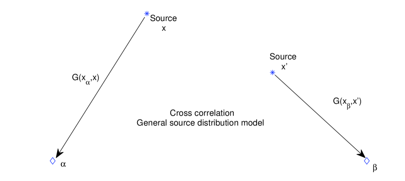
Figure 1: Cross correlations from a general model of sources as stated in equation (9). The source at ${\bf x}$ excites waves that propagate to $\alpha$ and the source at ${{\bf x}}^{\prime}$ generates waves that propagate to $\beta$. Because the sources themselves are statistically correlated, the expectation value of the wavefield cross correlation measured at points ${\bf x}_{\alpha},{\bf x}_{\beta}$ is non-trivial. Note that if the sources at two spatial points were statistically independent, the expectation value of the cross correlation would be zero when ${\bf x}\neq{\bf x}^{\prime}$, as shown in Figure 2. This form of source distribution is useful in modeling, e.g., storms, which can move substantial distances over relatively short times.

which allows us to construct forward models of cross correlation, a first step towards inversions.

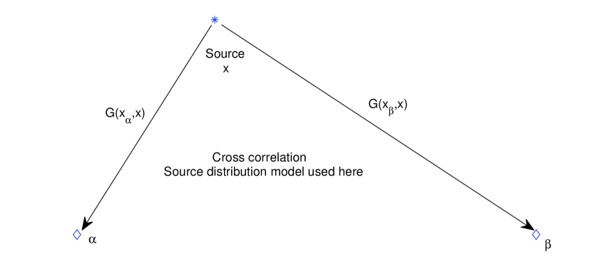
Figure 2: Cross correlations due to the distribution with $\langle S^{*}({\bf x},\omega)\,S({\bf x}^{\prime},\omega)\rangle={\mathcal{P}}(\omega)\,\sigma({\bf x})\,\delta({\bf x}-{\bf x}^{\prime})$, as described in equation (10). This model renders feasible the prediction or forward computation of the cross correlations because of the reduction in the number of integration variables. The inverse problem is also more easily dealt with since the number of degrees of freedom is much smaller.

Substituting Green’s function (6) into (10), we obtain

$$\langle{\mathcal{C}}_{\alpha\beta}\rangle=\int d{\bf x}\,H_{0}^{(2)}\left(\frac{\omega}{c}|{\bf x}_{\alpha}-{\bf x}|\right)\,H_{0}^{(1)}\left(\frac{\omega}{c}|{\bf x}_{\beta}-{\bf x}|\right)\,{\mathcal{P}}\,\sigma({\bf x}),$$ (11)

where the Hankel function of the second kind is defined thus $H_{0}^{(2)}=H_{0}^{(1)*}$. For convenience, we also define $\Delta_{\alpha}=|{\bf x}_{\alpha}-{\bf x}|$.

3 Structure of Source Kernels

Sensitivity kernels for noise distributions were introduced by Tromp et al. (2010), who termed them ensemble kernels. Consider the inverse problem where we are interested solely in the source distribution, i.e., variations of the correlation are rooted only in variations of the source distribution (as opposed to a more complete inverse problem which would contain variations to structure as well)

$$\delta\langle{\mathcal{C}}_{\alpha\beta}\rangle=\langle\delta{\mathcal{C}}_{\alpha\beta}\rangle=\int d{\bf x}\,H_{0}^{(2)}\left(\frac{\omega}{c}\Delta_{\alpha}\right)\,H_{0}^{(1)}\left(\frac{\omega}{c}\Delta_{\beta}\right)\,{\mathcal{P}}\,\delta\sigma({\bf x}).$$ (12)

Suppose the measurable $\delta{\mathcal{F}}$, such as a travel time or energy, is locally a linear functional of the variation of the cross correlation, i.e.,

$$\delta{\mathcal{F}}=\int d\omega\,W^{*}_{\alpha\beta}\,\langle\delta{\mathcal{C}}_{\alpha\beta}\rangle,$$ (13)

where $W_{\alpha\beta}(\omega)$ is some weight function. Then we have

$$\delta{\mathcal{F}}=\int d{\bf x}\left[\int d\omega\,W^{*}_{\alpha\beta}\,H_{0}^{(2)}\left(\frac{\omega}{c}\Delta_{\alpha}\right)\,H_{0}^{(1)}\left(\frac{\omega}{c}\Delta_{\beta}\right)\right]{\mathcal{P}}\,\delta\sigma({\bf x}),$$ (14)

where it may be seen that the term within the square brackets is the source kernel $K_{\alpha\beta}({\bf x})$

$$K_{\alpha\beta}({\bf x})=\int d\omega\,W^{*}_{\alpha\beta}\,H_{0}^{(2)}\left(\frac{\omega}{c}\Delta_{\alpha}\right)\,H_{0}^{(1)}\left(\frac{\omega}{c}\Delta_{\beta}\right)\,{\mathcal{P}},$$ (15)

which is the sensitivity to variations in the amplitude of the source distribution. With a little help from asymptotics, we can immediately perceive the structure of this kernel. The far-field approximation to Hankel functions, i.e., for large values of the argument, is

$$H_{0}^{(1)}(z)\sim\frac{2}{\sqrt{\pi z}}\exp\left(iz-i\frac{\pi}{4}\right),\,\,\,\,|z|\rightarrow\infty.$$ (16)

Thus, were there to be no source activity at very low temporal frequency, at a distance of several wavelengths away from the measurement locations ${\bf x}_{\alpha,\beta}$, we may write

$$H_{0}^{(1)}\left(\frac{\omega}{c}\Delta_{\beta}\right) \sim \sqrt{\frac{2c}{\pi\omega\Delta_{\beta}}}\exp\left(\frac{i\omega}{c}\Delta_{\beta}-i\frac{\pi}{4}\right),$$ (17)

$$H_{0}^{(2)}\left(\frac{\omega}{c}\Delta_{\alpha}\right) \sim \sqrt{\frac{2c}{\pi\omega\Delta_{\alpha}}}\exp\left(-\frac{i\omega}{c}\Delta_{\alpha}+i\frac{\pi}{4}\right).$$ (18)

Substituting these asymptotic relations into the expression for the kernel in equation (15), we obtain the far-field limit

$$K_{\alpha\beta}({\bf x})\sim\frac{1}{\sqrt{\Delta_{\alpha}\Delta_{\beta}}}\,\frac{1}{2\pi}\int d\omega\,{\hat{f}}(\omega)\,\exp\left[-i\omega\frac{\Delta_{\alpha}-\Delta_{\beta}}{c}\right],$$ (19)

where ${\hat{f}}(\omega)=4\,c\,W^{*}_{\alpha\beta}\,{\mathcal{P}}\,/\omega$. Comparing this to the definition of the inverse Fourier transform (42), we conclude that

$$K_{\alpha\beta}({\bf x})\sim{f\left(\frac{\Delta_{\alpha}-\Delta_{\beta}}{c}\right)}\frac{1}{\sqrt{\Delta_{\alpha}\Delta_{\beta}}},$$ (20)

and the source-distribution kernel is also a function of the path difference between a given point and the two stations, shown in Figure 3. This relationship suggests the existence of hyperbolic features in the kernels, i.e., contours along which $(\Delta_{\alpha}-\Delta_{\beta})/c=(|{\bf x}-{\bf x}_{\alpha}|-|{\bf x}-{\bf x}_{\beta}|)/c=C$ is constant (also see, e.g., Snieder, 2004; Roux et al., 2005; Cupillard et al., 2011). The presence of the term $1/\sqrt{\Delta_{\alpha}\Delta_{\beta}}$ results in a much greater sensitivity to regions close to the station and the path joining the stations. In comparison, the source kernel possesses relatively weak sensitivity to areas away from this line. Since we have assumed that the source distribution is spatially uncorrelated, contributions that constructively add to the expected value of the cross correlation can only be from the same point in the source distribution. In other words, a source excites a waves at ${\bf x}$, which propagate to ${\bf x}_{\alpha,\beta}$ as described by Green’s functions between the two stations and the source location. The cross correlation thus registers the travel-time difference between a source point and the two stations, which remains constant along hyperbolae whose foci are the two stations. Source kernels are relatively easy to compute since there are no scattering terms. When including scattering, variations of Green’s function come in to play, and a Born expansion is required to determine the variation of Green’s functions.

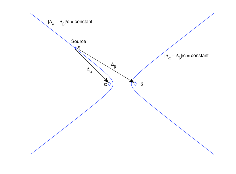
Figure 3: Contours of constant path difference are hyperbolae whose foci are the two stations ${\bf x}_{\alpha},{\bf x}_{\beta}$. For a given time-lag measurement of the cross correlation (i.e., choice of measurement time window), sources along the hyperbola constructively contribute to it.

An interesting analogy to note is that between scattering in the classical tomographic case (banana-doughnut kernels) and the source-amplitude kernel in the cross-correlation scenario. We will not go into mathematical detail but in both of these cases, two Green’s functions participate in the construction of the kernels. The sole difference between these two scenarios is that the source-amplitude kernel consists of a correlation between two Green’s functions and the scattering kernel is composed of a convolution between Green’s functions (e.g., Marquering et al., 1999). The source-amplitude kernel in the cross correlation case is thus analogous to anti-causal scattering in the classical case since one of the two Green’s functions has a complex conjugate in the cross-correlation case. The correlation/convolution difference changes the character of the kernel: elliptical features are observed in classical banana-doughnut kernels (e.g., Marquering et al., 1999) whereas hyperbolic features are seen in the cross-correlation source-amplitude kernels (also see, Gizon & Birch, 2002). Equation (15) for the classical scattering analog would then be

$$K^{\mathrm{C}S}_{\alpha\beta}({\bf x})=\int d\omega\,W^{*}_{\alpha\beta}\,H_{0}^{(1)}\left(\frac{\omega}{c}\Delta_{\alpha}\right)\,H_{0}^{(1)}\left(\frac{\omega}{c}\Delta_{\beta}\right),$$ (21)

where now this represents a convolution (note that both are Hankel functions of the first kind) and where $K^{\mathrm{C}S}_{\alpha\beta}({\bf x})$ is a classical scattering kernel. Applying the same asymptotic analysis, we obtain

$$K^{\mathrm{C}S}_{\alpha\beta}({\bf x})\sim{f\left(\frac{\Delta_{\alpha}+\Delta_{\beta}}{c}\right)}\frac{1}{\sqrt{\Delta_{\alpha}\Delta_{\beta}}},$$ (22)

which will produce elliptical features since these are contours of constant path length, i.e., where $(\Delta_{\alpha}+\Delta_{\beta})/c=(|{\bf x}-{\bf x}_{\alpha}|+|{\bf x}-{\bf x}_{\beta}|)/c=C$.

3.1 Computing Kernels

In this section, we discuss the structure of source-amplitude kernels through the exact computation of equations (11) and (15). The formulation used in this section follows from that of Dahlen & Baig (2002). We begin the process of computing kernels by defining a misfit functional $\chi$ in terms of the measured energy anomaly,

$$\chi=\frac{1}{2}\sum_{\alpha,\beta}\left(\ln\frac{A^{\rm obs}_{\alpha\beta}}{A^{\rm syn}_{\alpha\beta}}\right)^{2},$$ (23)

where the energy is defined as

$$A^{\rm syn}_{\alpha\beta}=\sqrt{\frac{\int dt\,\,w(t)\,\langle{\mathcal{C}_{\alpha\beta}(t)}\rangle^{2}}{\int dt\,w(t)}}=\sqrt{\frac{1}{2\pi T}\int d\omega\,\langle{\mathcal{C}}^{*}_{\alpha\beta}\rangle\,\langle{\mathcal{C}}_{\alpha\beta}\rangle},$$ (24)

where $w(t)$ is the windowing function, ${\mathcal{C}}_{\alpha\beta}$ is the windowed cross correlation and $T=\int dt\,w(t)$. Note that we use the term energy interchangeably with amplitude. To preserve simplicity, we do not apply frequency filters, although they may be easily included. In general, although we may compute sensitivity kernels for other measurements such as travel times, we restrict ourselves here to the cross correlation energy. With a little manipulation, not shown here, the variation in misfit is given by

$$\delta\chi=-\sum_{\alpha,\beta}\left(\ln\frac{A^{\rm obs}_{\alpha\beta}}{A^{\rm syn}_{\alpha\beta}}\right)\frac{\delta A^{\rm syn}_{\alpha\beta}}{A^{\rm syn}_{\alpha\beta}}=-\sum_{\alpha,\beta}\left(\frac{1}{A^{\rm syn}_{\alpha\beta}}\right)^{2}\left(\ln\frac{A^{\rm obs}_{\alpha\beta}}{A^{\rm syn}_{\alpha\beta}}\right)\frac{1}{2\pi T}\int d\omega\,\langle{\mathcal{C}}_{\alpha\beta}^{*}\rangle\,\langle\delta{\mathcal{C}}_{\alpha\beta}\rangle.$$ (25)

If one were to, as before, assume that the variations in the cross correlation only arose from changes to the source distribution,

$$\langle\delta{\mathcal{C}}_{\alpha\beta}\rangle=\int d{\bf x}\,G^{*}(\Delta_{\alpha})\,G(\Delta_{\beta})\,{\mathcal{P}}(\omega)\,\delta\sigma({\bf x}).$$ (26)

Thus defining the weight function as

$$W_{\alpha\beta}=\frac{1}{T}\,\left(\frac{1}{A^{\rm syn}_{\alpha\beta}}\right)^{2}\langle{{\mathcal{C}}}_{\alpha\beta}\rangle,$$ (27)

variations to the misfit functional are then described by

$$\delta\chi=-\sum_{\alpha,\beta}\left(\ln\frac{A^{\rm obs}_{\alpha\beta}}{A^{\rm syn}_{\alpha\beta}}\right)\int d{\bf x}\,K_{\alpha\beta}({\bf x})\,\delta\sigma({\bf x}).$$ (28)

The kernel normalization is tested by confirming that the following integral is satisfied

$$\int d{\bf x}\,K_{\alpha\beta}({\bf x})\,\sigma({\bf x})=\left(\frac{1}{A^{\rm syn}_{\alpha\beta}}\right)^{2}\,\frac{1}{2\pi T}\int d\omega\,{\langle{\mathcal{C}}}^{*}_{\alpha\beta}\rangle\int d{\bf x}\,G^{*}(\Delta_{\alpha})\,G(\Delta_{\beta})\,{\mathcal{P}}(\omega)\,\sigma({\bf x})=1$$ (29)

(obtained upon applying definition (24) for the energy and equation (10) for the expected cross correlation).

We compute source-amplitude kernels (around a uniform distribution $\sigma=1$) in the temporal Fourier domain, using the exact functional form of Green’s function (6). The wavespeed is set to $c=1$ km/s. The expected (limit) cross correlation contains symmetric positive and negative branches. The power spectrum and its temporal representation are shown in Figure 4. We use a temporal grid of 401 points and the frequency spacing of 0.05 Hz, and hence a time window of 20 seconds, as in Figure 4. The spacing in the temporal grid is 0.05 seconds, implying a Nyquist frequency of 10 Hz. In order to compute the integral over frequency in equation (15), we precompute Hankel functions on a grid of $681\times 681$ points resolving a square of size $[-40,40]\times[-40,40]$ km². These function values are then utilized to compute the expected cross correlation and kernels. For the examples in Figure 5, we choose $\sigma({\bf x})=1$, i.e., a uniform distribution. In Figure 5, we show examples of how the choice of the measurement affects the sensitivity kernel. On the upper panels, the expected cross correlation for a point pair separated by a distance of 10.6 km. The dashed box indicates the choice of measurement, a 4 second window on the left panel and a 0.5 second window on the right. Kernels corresponding to these choices are shown immediately below. A thicker hyperbola, indicative of a broader range of path differences, is seen on the kernel to the left (compared with the thinner hyperbolae on the right). Because we choose only the positive branch, the kernel shows sensitivity only to waves that first arrive at the station on the left and subsequently to the one on the right. Consequently, the hyperbolae point to the left.

In general, the source-amplitude kernel depends indirectly on the choice of the initial spatial distribution of sources. Firstly, the cross correlation is obtained by evaluating an integral involving the spatial source distribution over space (Eq. [11]). This predicted cross correlation is then used in the computation of the kernel (Eqs. [15] and [27]). The function $W_{\alpha\beta}$, from equation (27), assigns a frequency-dependent weight to the two Green’s functions in the integral (15). But since Green’s functions are an inseparable mix of frequency and space (see Eq. [6]), the kernel resulting from the evaluation of (15) will possess a spatial dependence that reflects the source distribution.

Source-amplitude kernels as a function of interstation distance are graphed in Figure 6. It is seen that at small distances, the lateral size of the kernel is comparable to the interstation distance whereas at very large distances, the sensitivity is restricted to a small range of azimuths around the interstation path. There are disadvantages to using measurements at stations separated by small distances since they are only able to image the source distribution in their vicinity, leading possibly to errors in the inversion. Further, if the distance between the stations is less than a wavelength, the cross correlation does not provide very much additional information and should be removed from the analysis.

In Figure 7, we show kernels as a function of interstation distance and the temporal frequency of the measurement. Higher-frequency waves lead to kernels with greater complexity and spatially sharper features. Much as in classical tomography, finer-scale images of the source distribution may be obtained by using higher-frequency measurements. It is unclear how useful this will be when attempting to invert for oceanic microseisms since they occur at narrow frequency bands. In other words, if one were to incorporate higher or lower frequency measurements, away from the central microseism excitation frequency, would be of very limited utility in imaging. A more thorough study is needed in this regard.

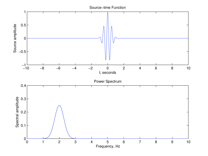
Figure 4: Source-time function (upper panel) and the power spectrum ${\mathcal{P}}(\omega)$.

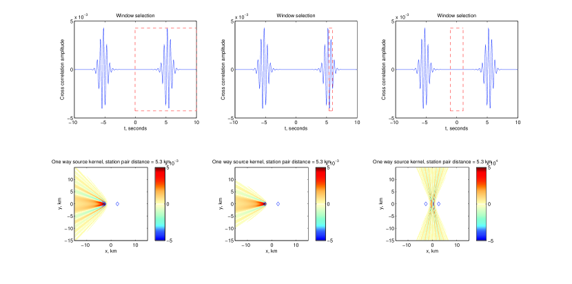
Figure 5: Expected cross correlation (upper panels) and the attendant kernels (bottom panels). Stations are marked by the diamond symbols. A wider measurement window implies that the the hyperbolae are thicker, as can be seen upon comparing lower left and middle panels. Note that when the window straddles the zero time lag part of the cross correlation, the kernel will show sensitivity to sources along the bisecting line perpendicular to the path between the stations (bottom right). The part of the kernel along the line joining the two stations (i.e., $y=0$) is sensitive to parts of the cross correlation corresponding to late times whereas the hyperbolae closest to the bisector (i.e., $x=0$) are due to the zero-time-lag part of the cross correlation. The color scale has been saturated so as to enhance the visibility of the relatively weak hyperbolae.

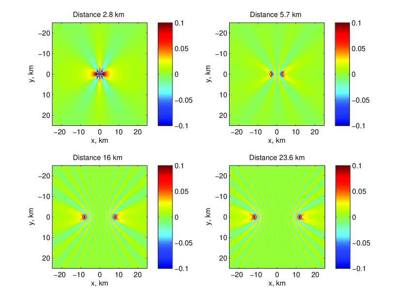
Figure 6: Source kernels as a function of interstation distance for a uniform source distribution. The measurement is the energy of the entire waveform. At small distances, the lateral size of the kernel is comparable to the interstation distance whereas at very large distances, the sensitivity is restricted to a small range of azimuths around the interstation path.

Figure 7: Source kernels as a function of frequency of the measurement. The source-time functions used in computing the two sets of kernels are plotted on the bottom two panels. The measurement is the energy of the entire waveform. When we use a more rapidly varying source-time function (right column), the kernel shows greater complexity and spatially sharper features. Much as in classical tomography, finer-scale images of the source distribution may be obtained by using higher-frequency measurements.

3.2 Non-uniform source distribution and the event kernel

The presence of strong non-uniformities can render inaccurate results pertaining to the correspondence between the cross correlation measurement and Green’s functions along the station pair. The integral in (11) is over all space and provided the weight function $\sigma({\bf x})$ is also uniform, the expectation value of the cross correlation is well behaved, displaying features similar to classical tomographic arrivals, an instance of which is shown on the upper panels of Figure 8. In fact, for the case considered here, the expected cross correlation can be shown to be a frequency modulation of Green’s functions along the path (without wave attenuation; see Tromp et al., 2010). However, when the source distribution $\sigma$ becomes more non-uniform, the expectation value of the cross correlation shifts away from the elegant Green’s function analog and adopts more complicated forms. A particularly stark example is when the sources lie along the bisector line perpendicular to the path between the station-pair: the cross correlation in such a case will be centered around zero time, since the path difference from the source to the stations is zero. We also consider a situation that has been studied extensively in past literature (e.g., Derode et al., 2003; Larose et al., 2006; Fleury et al., 2010), namely that of a ring of sources surrounding a station pair. Indeed, we find in Figure 9 that the cross correlation owing to a uniform distribution of sources is almost identical to that in the ring of sources scenario. As opposed to a discrete number of sources placed at a certain radius around the station pair, we use a continuous annulus to represent the ring. The amplitude of the uniform distribution is substantially smaller in order that the cross correlations from these two situations have the same energy.

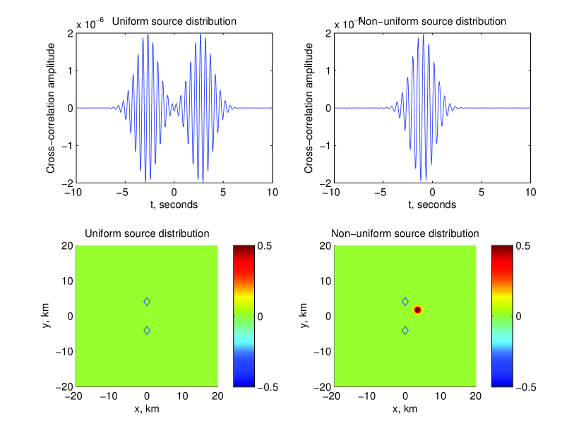
Figure 8: Expected cross correlation (upper panels) and the source distributions (bottom panels). Stations are marked by the diamond symbols. Pathological distributions (such as the lower right) of sources can cause large shifts in the expectation value of the cross correlation because of the non-uniform manner in which waves illuminate the stations. In this case, the only source being the spot, is very close to the bisector line perpendicular to the path between the stations (i.e., $y=0$), implying that the path difference between the spot and the stations is nearly zero. The cross correlation is thus almost (but not quite) centered around zero time.

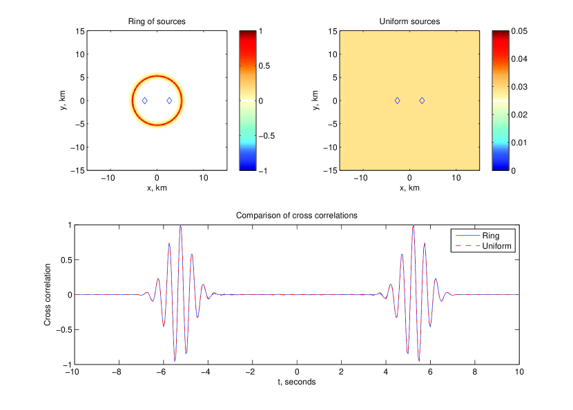
Figure 9: The celebrated “ring of sources surrounding a station pair” scenario (left panel) and uniform distribution of weaker amplitude (right panel). Cross correlations at the stations (symbols) due to these distributions are over plotted (bottom panel). They are practically indistinguishable, and is part of the reason why the ring configuration of sources has been studied so extensively.

In Figure 10, we make the case for the imaging of anisotropic source distributions. The “true” distribution is shown on the left panel. The starting “synthetic” model consists of a uniform distribution of sources whose amplitude is the same as that of the “true” distribution away from the local spot of increased amplitude on the south-east quadrant. We use the energy of the full envelope of the cross correlation, from zero to the classical surface-wave arrival time. We compute the misfit according to equation (23). The event kernel associated with a particular station $\alpha$ is a sum of the point-to-point kernels between that station and all other stations, i.e.,

$$K_{\alpha}({\bf x})=\sum_{\beta}\ln\frac{A^{\rm obs}_{\alpha\beta}}{A^{\rm syn}_{\alpha\beta}}\,K_{\alpha\beta}({\bf x}),$$ (30)

where $A^{\rm obs}$ signifies the “true” energies. The sum of all the event kernels associated with a network of stations provides a way to update the model, and is $\sum_{\alpha}K_{\alpha}({\bf x})$. As discussed in Tromp et al. (2010), the cost of the inversion scales with the number of “master” pixels $\alpha$ and is independent of the number of “slaves” $\beta$. However because we use a translationally invariant background model, the computation of kernels is cheap and so we may include as many master pixels as we desire. In this case, we stop at 20 stations, i.e., 20 master and 19 slave pixels.

In Figure 10, we show the sum of event kernels corresponding to this set of “data” and “synthetics”. The kernels neatly focus onto the area where the source amplitude is locally large (by 500% in comparison to the value away from this spot). In order to image this localized spot better, we would require a greater coverage by the array, i.e., an array that surrounds the spot, as shown in Figure 11. Note that the farther away the anomalous source activity is from the array, thus diminishes the ability to discern their location. An example of such a situation is shown in Figure 12. One may interpret it as the sources being far enough away that when the waves arrive at the stations, their curvature ($\propto\Delta_{S}^{-1}$, $\Delta_{S}$ being the distance from the source) is so small that they appear as plane waves, and information about the source location is thus lost. In order to perceive such small curvature, a network of stations placed far apart ($\propto\Delta_{S}$) becomes necessary. An additional reason for the spatially localized sensitivity is that the source kernel is of greatest amplitude along the interstation paths and in the vicinities of the stations. Conceptually, imaging of the noise source distribution is not very different from that of inverting for an earthquake source; both require appropriate choices for measurements and a good network of stations. Subsequently, by studying the inverted source distribution, we may arrive at the conclusion that the distribution is too far away to image. In this case the procedure is essentially no different from beamforming (e.g., Stehly et al., 2006). However, if there were to be more information in the wavefield (by using different time windows and some intrinsic curvature properties of the waves), then this method will be able to utilize it to produce better quality images of the noise source distribution than beamforming.

Rapid temporal variations in the source distribution may also be lost when the cross correlations are averaged over long times. However, this is independent of the technique used, i.e., beamforming or an adjoint method (used here). Therefore it is useful to apply the sorts of methods described here since it maximally utilizes wavefield information.

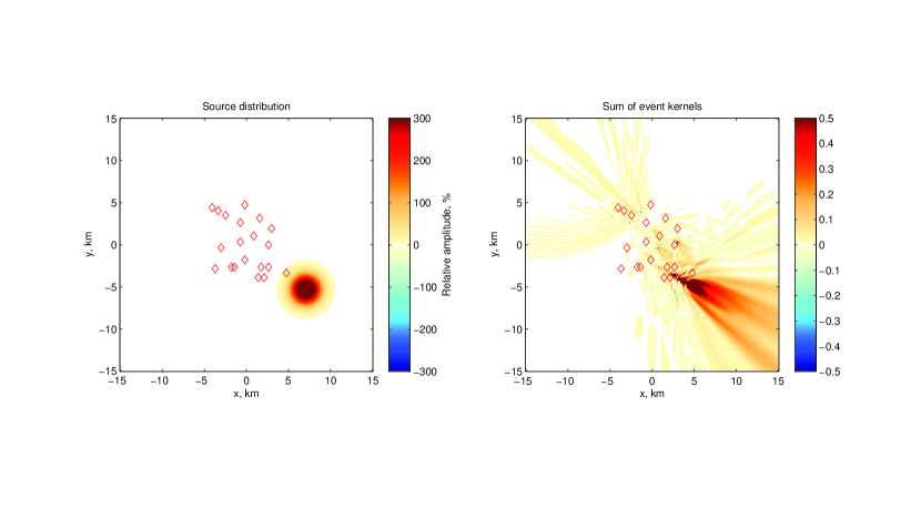
Figure 10: Sum of event kernels. The left panel shows the “true” source distribution, with respect to a nominal (uniform) value. Stations are marked by symbols. It contains a local spot of relatively large amplitude (500% increase over the uniform value) on the south-east quadrant. Because of the relative proximity of the station array to the sources, the event kernel is able to roughly localize over the spot. Since there is no coda (and complex structure) in this simple test case, the window encompasses the entire waveform. Thus the energy of the entire cross correlation contributes to the construction of the image of the noise source distribution.

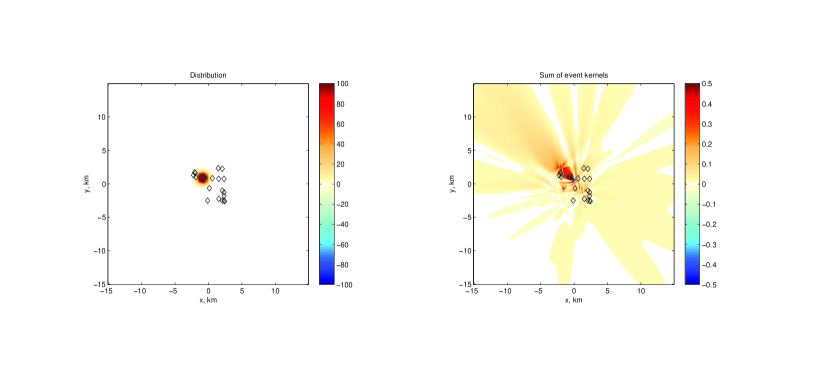
Figure 11: Sum of event kernels. The left panel shows the “true” source distribution, with respect to a nominal (uniform) value. Stations are marked by symbols. We include a local spot of relatively large amplitude (200% increase over the uniform value) amid the station array. Because stations surround the anomaly, they are able to accurately locate the distribution. Since there is no coda (and complex structure) in this simple test case, the window encompasses the entire waveform. Thus the energy of the entire cross correlation contributes to the construction of the image of the noise source distribution.

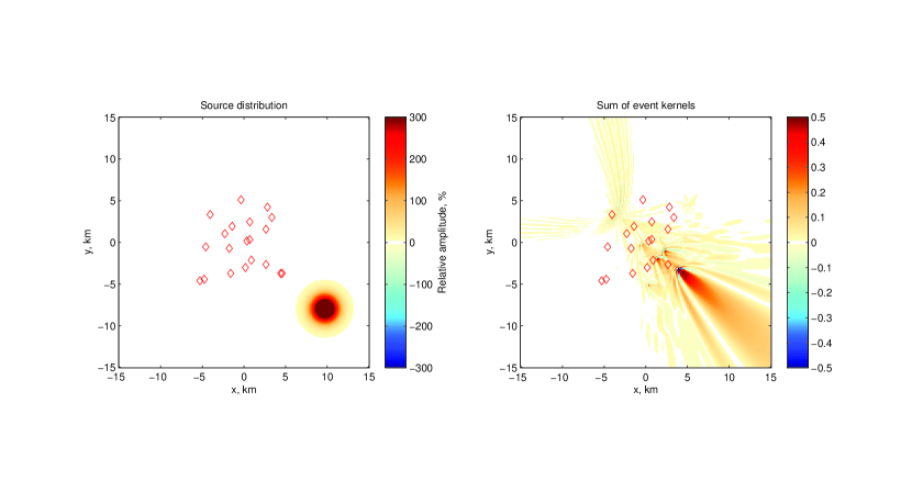
Figure 12: Sum of event kernels. The left panel shows the “true” source distribution, with respect to a nominal (uniform) value. Stations are marked by symbols. We include a local spot of relatively large amplitude (500% increase over the uniform value) moved farther away from the station array than in Figure 10. Evidently, the stations are too far away from the sources to accurately locate the distribution. Since there is no coda (and complex structure) in this simple test case, the window encompasses the entire waveform. Thus the energy of the entire cross correlation contributes to the construction of the image of the noise source distribution.

4 Scattering

In the framework of correlation tomography, scattering kernels can be substantially more complicated. They are also intrinsically different in flavor from classical banana-doughnut kernels, containing additional hyperbolic features which represent sensitivity to sources at disparate spatial locations. Much as in Figures 1 and 2, we attempt here to graphically explain the physics of scattering kernels for noise measurements.

Variations to the limit cross correlation (3) are given by

$$\langle\delta{\mathcal{C}}_{\alpha\beta}\rangle=\langle\phi^{*}({\bf x}_{\alpha})\,\delta\phi({\bf x}_{\beta})\rangle+\langle\delta\phi^{*}({\bf x}_{\alpha})\,\phi({\bf x}_{\beta})\rangle+O(\delta\phi^{2}),$$ (31)

in which, keeping with convention, we do not explicitly state the dependence on frequency $\omega$. Hitherto, we have ignored scattering terms but in this section, we describe their mathematical structure. For a given wave operator ${\mathcal{L}}$ and the corresponding wavefield $\phi$ satisfying

$${\mathcal{L}}\phi=S,$$ (32)

the first Born approximation (e.g., Hudson, 1977; Wu & Aki, 1985) describing the singly scattered wavefield $\delta\phi$ owing to perturbations to the operator, $\delta{\mathcal{L}}$, is

$$\delta({\mathcal{L}}\phi)={\mathcal{L}}\delta\phi+\delta{\mathcal{L}}\phi=0,$$ (33)

where we assume that the source distribution is known exactly. We have

$${\mathcal{L}}\delta\phi=-\delta{\mathcal{L}}\phi,$$ (34)

which upon using Green’s theorem (Eq. [7]) for the wavefield, we obtain

$$\delta\phi({\bf x})=-\int d{\bf x}{{}^{\prime\prime}}G({\bf x},{\bf x}{{}^{\prime\prime}})[\delta{\mathcal{L}}\phi],$$ (35)

where $\phi=\phi({\bf x}{{}^{\prime\prime}})$ and which may be rewritten in terms of the source distribution $S({\bf x}^{\prime})$ as

$$\delta\phi({\bf x})=-\int d{\bf x}{{}^{\prime\prime}}G({\bf x},{\bf x}{{}^{\prime\prime}})\,\delta{\mathcal{L}}\left(\int d{\bf x}^{\prime}\,G({\bf x}{{}^{\prime\prime}},{\bf x}^{\prime})\,S({\bf x}^{\prime})\right).$$ (36)

This equation states that a source creates a wave at ${\bf x}^{\prime}$, which propagates to a point ${\bf x}{{}^{\prime\prime}}$ as described by Green’s function along that path, is singly scattered according to $\delta{\mathcal{L}}$ and subsequently acts as a source, eventually propagating to measurement point ${\bf x}$. This is the framework in which classical tomographic scattering is studied (shown in Figure 13). Substituting this into equation (31),

$$\langle\delta{\mathcal{C}}_{\alpha\beta}\rangle=-\langle\left[\int d{\bf x}\,G^{*}({\bf x}_{\alpha},{\bf x})\,S^{*}({\bf x})\right]\left\{\int d{\bf x}{{}^{\prime\prime}}G({\bf x}_{\beta},{\bf x}{{}^{\prime\prime}})\,\delta{\mathcal{L}}\left(\int d{\bf x}^{\prime}\,G({\bf x}{{}^{\prime\prime}},{\bf x}^{\prime})\,S({\bf x}^{\prime})\right)\right\}\rangle$$ (37)

$$\mbox{}-\langle\left\{\int d{\bf x}{{}^{\prime\prime}}G^{*}({\bf x}_{\alpha},{\bf x}{{}^{\prime\prime}})\,\delta{\mathcal{L}}^{*}\left(\int d{\bf x}^{\prime}\,G^{*}({\bf x}{{}^{\prime\prime}},{\bf x}^{\prime})\,S^{*}({\bf x}^{\prime})\right)\right\}\left[\int d{\bf x}\,G({\bf x}_{\beta},{\bf x})\,S({\bf x})\right]\rangle.$$

The terms in the flower brackets denote the scattering contributions and the terms within the square brackets show the direct wave arrival from the source to the observation points. Because we truncate the Born approximation to one term, i.e., considering only contributions from single scattering processes, the variation of the cross correlation consists of a direct wave propagating from a source to one of the stations, correlated with a singly scattered wave that propagates to the other measurement point. Akin to Gizon & Birch (2002), we diagrammatically show the formal interpretation of the measurement in Figure 14. In contrast to single-scattering theory applied to classical tomographic wavefield measurements (shown in Figure 13), in which two Green’s functions appear, the higher-order correlation measurement (regardless of whether these are “noise” or earthquake sources) requires the evaluation of three Green’s functions.

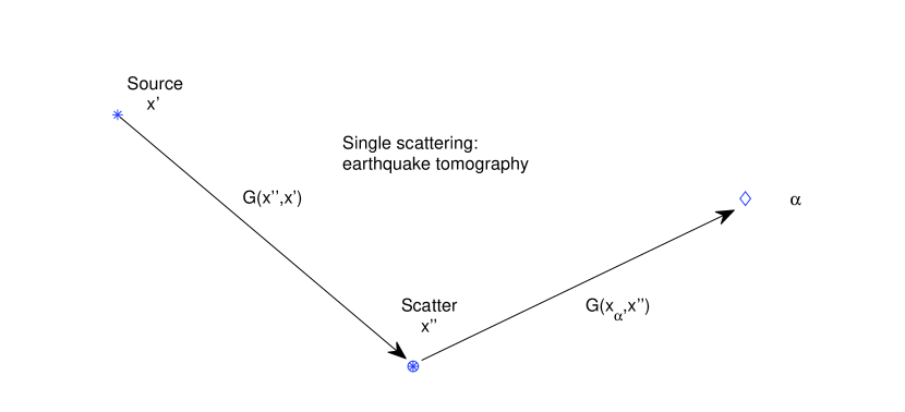
Figure 13: Single scattering in the classical earthquake tomography case. A source at ${{\bf x}^{\prime}}$ excites a wave that propagates to ${\bf x}{{}^{\prime\prime}}$ where it scatters, acts as a source, propagating finally to station $\alpha$. It is substantially simpler than the cross correlation measurement, which is depicted in Figures 14 and 15. Only two Green’s functions are required to model single scattering in this scenario.

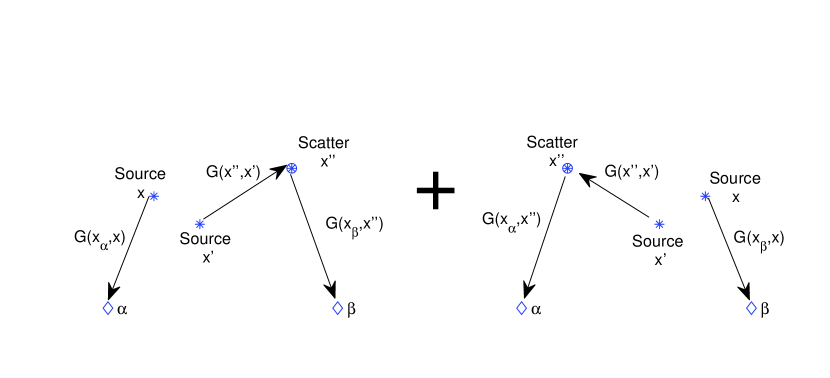
Figure 14: Scattering as captured by cross correlations for a general source distribution (similar to Figure 1) with non-zero spatial covariance. The first contribution (first line of Eq. [37]) consists of a correlation between a wave generated at point ${\bf x}$, propagated to $\alpha$ and a wave generated at ${\bf x}^{\prime}$, scattered according to perturbation $\delta{\mathcal{L}}$ at point ${\bf x}{{}^{\prime\prime}}$, propagated to measurement point $\beta$. The second contribution (second line of Eq. [37]) is essentially the same except with points $\alpha,\beta$ reversed. This is the reason why three Green’s functions are needed to formally interpret the measurement in terms of single-scattering theory.

Upon invoking the assumption of spatially uncorrelated sources, i.e., $\langle S({\bf x})\,S^{*}({\bf x}^{\prime})\rangle=\delta({\bf x}-{\bf x}^{\prime})\,\sigma({\bf x})\,{\mathcal{P}}(\omega)$, we obtain

$$\langle\delta{\mathcal{C}}_{\alpha\beta}\rangle=-\int d{\bf x}{{}^{\prime\prime}}G({\bf x}_{\beta},{\bf x}{{}^{\prime\prime}})\,\delta{\mathcal{L}}\left(\int d{\bf x}^{\prime}\,G({\bf x}{{}^{\prime\prime}},{\bf x})\,G^{*}({\bf x}_{\alpha},{\bf x})\,\sigma({\bf x})\,{\mathcal{P}}\right)$$ (38)

$$\mbox{}-\int d{\bf x}{{}^{\prime\prime}}G^{*}({\bf x}_{\alpha},{\bf x}{{}^{\prime\prime}})\,\delta{\mathcal{L}}^{*}\left(\int d{\bf x}\,G^{*}({\bf x}{{}^{\prime\prime}},{\bf x})\,G({\bf x}_{\beta},{\bf x})\,\sigma({\bf x})\,{\mathcal{P}}\right),$$

which produces a scattering diagram similar to Figure 14, except with coinciding points ${\bf x},{\bf x}^{\prime}$, as shown in Figure 15. These kernels are indeed more difficult to compute than in the classical tomography case, and evidently require the evaluation of three Green’s functions. The physics of these kernels is also conceptually different from the classical case.

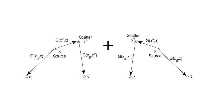
Figure 15: Scattering as captured by cross correlations for a source distribution with zero spatial covariance (similar to Figure 2) . The first contribution (first line of Eq. [38]) consists of a correlation between a wave generated at point ${\bf x}$ propagated to points $\alpha$ and ${\bf x}{{}^{\prime\prime}}$, with the latter scattered according to perturbation $\delta{\mathcal{L}}$ at point ${\bf x}{{}^{\prime\prime}}$ and eventually propagated to measurement point $\beta$. The second contribution (second line of Eq. [38]) is essentially the same except with points $\alpha,\beta$ reversed. This is the reason why three Green’s functions are needed to formally interpret the measurement in terms of single-scattering theory. The only difference between this figure and Figure 14 is that the contributions to the cross correlation are from the same source point (i.e., when ${\bf x}={\bf x}^{\prime}$).

5 The sensitivity of cross-correlation energies to attenuation

The topic of imaging wave attenuation using cross-correlation energies is a topic of interest (e.g., Cupillard & Capdeville, 2010; Weaver et al., 2011; Prieto et al., 2011; Tsai, 2011). The challenge is to accurately interpret enhanced decrements in cross-correlation energies amid effects of geometrical spreading with distance and wave-speed heterogeneities. Evidently, the distribution of sources significantly influences the conclusion of any inverse problem, and the problem of the determination of wave attenuation is no different. This suggests that the strategy typically followed in earthquake tomography, which is to first invert for the source and subsequently for structure (perhaps iteratively), may be applied equally to noise measurements. The standard trade-off between source and structure affects the interpretation of noise measurements as well.

In Figure 16, we show the variation in energy (defined as the energy of the cross-correlation branch (24), positive or negative) of the cross correlation as a function of distance between the station pair for three source distributions. The variation in energy is entirely due to geometrical spreading and source distribution anisotropies. Note that the background model has no attenuation in this case. The scatter in cross correlation energies for the anisotropic case may possibly be reduced by choosing an azimuthally varying normalization (Prieto et al., 2009).

The ring of sources case is seen to be different from the uniform distribution. This is because the in an attenuating medium, sources from farther away contribute less to the cross correlation. Therefore, the cross correlation energies in the ring and uniform cases converge to different expectation values, whose difference increases with the extent of attenuation.

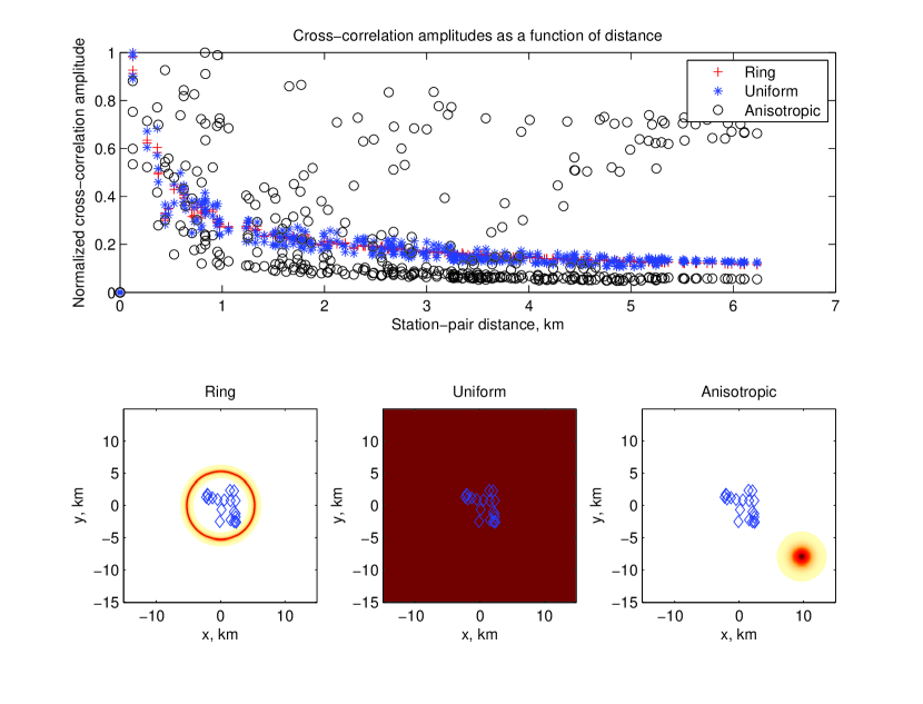
Figure 16: Cross-correlation energy (or amplitude; Eq. [24]) as a function of distance between station pairs (the network shown in the lower panels). Stations, marked by diamonds, are illuminated by a ring of sources (left), uniform sources (middle) and by a highly anisotropic distribution (right). The scatter in energies is entirely due to geometric spreading and source distribution anisotropy (for the anisotropic case). Amplitudes of every branch of every cross correlation are plotted (independent of orientation) in the upper panel for the three cases. They are normalized in all three cases such that the greatest value is 1. Determining the source distribution prior to interpretation is strongly tied to the accurate interpretation of these measurements. However, it may be noted that in the anisotropic case, the normalization could be chosen to be azimuthally dependent, resulting in energy shifts better suited to fitting (Prieto et al., 2009).

We also characterize the significance of a finite quality factor on energies when the network is illuminated by the source distributions of Figure 16. We use a damping rate of 0.01 Hz, or a quality factor of roughly 150. Wave attenuation is modeled via solutions of the damped simple harmonic oscillator, i.e., operator (4) with a damping term

$$\partial_{t}^{2}\phi+\Gamma\,\partial_{t}\phi-c^{2}\nabla^{2}\phi=0,$$ (39)

where attenuation $\Gamma$ has units of Hertz. Green’s function for this operator is then

$$G({\bf x},{\bf x}^{\prime})=\frac{i}{4}H^{(1)}\left(\frac{p\,\omega}{c}|{\bf x}-{\bf x}^{\prime}|\right),$$ (40)

where the factor $p=\sqrt{1+i\Gamma/\omega}$. Amplitudes evidently change but in entirely different ways, depending on the source distribution, as displayed in Figure 17. We show the percentage change in cross correlation energies due to the introduction of a spatially constant wave attenuation of 0.01 Hz. Figure 17 demonstrates that wave energies are indeed sensitive to attenuation, but extracting this information is subject to accurate knowledge of the source distribution.

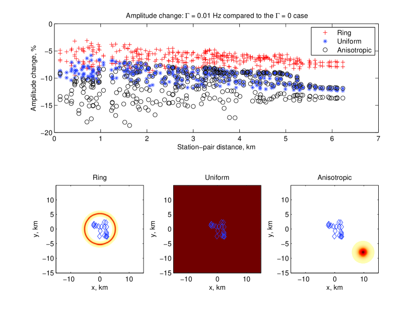
Figure 17: Change in energies (amplitudes) due to the introduction of wave attenuation of cross correlations for the network and source distributions of Figure 16. We use a damping rate of $\Gamma=0.01$ Hz. We plot the relative energy change of every branch of every cross correlation as a function of station-pair distance. The anisotropic distribution shows the largest changes in energies - and this is because upon introducing attenuation, waves which travel from the patch of sources arrive with diminished energies by the time they reach the network. The effect is less severe in the ring of sources case, where the ring is close to the network. In any case, the knowledge of the source distribution is critical to inferring properties of the underlying medium. In the scenario of a uniform distribution of sources (plus symbols), it certainly appears that the energy reduction due to attenuation is a robust effect and may be used in a straightforward manner to infer wave attenuation.

6 Conclusions

Cross correlations are intrinsically more complex than classically used wavefield displacements. There are fundamental and meaningful differences between these measurements, which have consequences for the eventual solution of inverse problems. Because seismology is a precision science, it is important to formally interpret these measurements and capture their essence as fully as possible. Using a simple 2-D example, we have endeavored to delve into the physics of the cross correlation measurement. A goal of this article was to demonstrate the utility and ease of studying distributions of sources and posing the problem in terms of the expectation value of the relevant measurable. We make a case for the imaging of source distributions using measurements of cross-correlation energies. The dependence of these energies on station-pair distance and on wave attenuation is also touched upon. The influence of the source distribution on the energy measurement is demonstrated; cross-correlation energies unquestionably contain information about wave attenuation (primarily within the network) but it is hard to interpret them accurately without knowledge of the sources.

Appendix A Fourier Convention

The following Fourier transform convention is utilized

$$\int_{-\infty}^{\infty}dt~{}e^{i\omega t}~{}g(t) = {\hat{g}}(\omega),$$ (41)

$$\int_{-\infty}^{\infty}dt~{}e^{i\omega t} = 2\pi~{}\delta(\omega),$$ (42)

$$\frac{1}{2\pi}\int_{-\infty}^{\infty}d\omega~{}e^{-i\omega t}~{}{\hat{g}}(\omega) = g(t),$$ (43)

$$\int_{-\infty}^{\infty}d\omega~{}e^{-i\omega t} = 2\pi~{}\delta(t),$$ (44)

where $g(t),{\hat{g}}(\omega)$ are a Fourier-transform pair. The equivalence between cross-correlations and convolutions in the Fourier and temporal domain are written so

$$h(t)=\int_{-\infty}^{\infty}dt^{\prime}~{}f(t^{\prime})~{}g(t+t^{\prime})\Longleftrightarrow{\hat{h}}(\omega)={\hat{f}}^{*}(\omega)~{}{\hat{g}}(\omega),\\$$ (45)

$$h(t)=\int_{-\infty}^{\infty}dt^{\prime}~{}f(t^{\prime})~{}g(t-t^{\prime})\Longleftrightarrow{\hat{h}}(\omega)={\hat{f}}(\omega)~{}{\hat{g}}(\omega).$$ (46)

The following relationship also holds (for real functions $f(t),g(t)$)

$$\int_{-\infty}^{\infty}dt~{}f(t)~{}g(t)=\frac{1}{2\pi}\int_{-\infty}^{\infty}d\omega~{}{\hat{f}}^{*}(\omega)~{}{\hat{g}}(\omega)=\frac{1}{2\pi}\int_{-\infty}^{\infty}d\omega~{}{\hat{f}}(\omega)~{}{\hat{g}}^{*}(\omega).$$ (47)

References

- Aki & Richards (1980) Aki, K. & Richards, P. G., 1980. Quantitative Seismology, Theory and Methods, W. H. Freeman, San Francisco, California, USA.
- Brenguier et al. (2007) Brenguier, F., Shapiro, N. M., Campillo, M., Nercessian, A., & Ferrazzini, V., 2007. 3-D surface wave tomography of the Piton de la Fournaise volcano using seismic noise correlations, Geophys. Res. Lett., 34, 2305.
- Brenguier et al. (2008) Brenguier, F., Campillo, M., Hadziioannou, C., Shapiro, N., Nadeau, R., & Larose, E., 2008. Postseismic relaxation along the san andreas fault at parkfield from continuous seismological observations, Science, 321(5895), 1478–1481.
- Chevrot et al. (2007) Chevrot, S., Sylvander, M., Benhamed, S., Ponsolles, C., Lefèvre, J., & Paradis, D., 2007. Source locations of secondary microseisms in western europe: Evidence for both coastal and pelagic sources, J. Geophys. Res., 112, B11301.
- Cupillard & Capdeville (2010) Cupillard, P. & Capdeville, Y., 2010. On the amplitude of surface waves obtained by noise correlation and the capability to recover the attenuation: a numerical approach, Geophysical Journal International, 181, 1687–1700.
- Cupillard et al. (2011) Cupillard, P., Stehly, L., & Romanowicz, B., 2011. The one-bit noise correlation: a theory based on the concepts of coherent and incoherent noise, Geophysical Journal International, 184, 1397–1414.
- Dahlen & Baig (2002) Dahlen, F. A. & Baig, A. M., 2002. Fréchet kernels for body-wave amplitudes, Geophysical Journal International, 150, 440–466.
- Derode et al. (2003) Derode, A., Larose, E., Tanter, M., de Rosny, J., Tourin, A., Campillo, M., & Fink, M., 2003. Recovering the Green’s function from field-field correlations in an open scattering medium (L), Acoustical Society of America Journal, 113, 2973–2976.
- Duvall et al. (1993) Duvall, Jr., T. L., Jefferies, S. M., Harvey, J. W., & Pomerantz, M. A., 1993. Time-distance helioseismology, Nature, 362, 430–432.
- Fichtner et al. (2006) Fichtner, A., Bunge, H.-P., & Igel, H., 2006. The adjoint method in seismology, Physics of the Earth and Planetary Interiors, 157, 86–104.
- Fleury et al. (2010) Fleury, C., Snieder, R., & Larner, K., 2010. General representation theorem for perturbed media and application to Green’s function retrieval for scattering problems, Geophysical Journal International, 183, 1648–1662.
- Froment et al. (2010) Froment, B., Campillo, M., Roux, P., Gouédard, P., Verdel, A., & Weaver, R., 2010. Estimation of the effect of nonisotropically distributed energy on the apparent arrival time in correlations, Geophysics, 75, SA85.
- Gizon & Birch (2002) Gizon, L. & Birch, A. C., 2002. Time-Distance Helioseismology: The Forward Problem for Random Distributed Sources, ApJ, 571, 966–986.
- Hanasoge et al. (2011) Hanasoge, S. M., Birch, A., Gizon, L., & Tromp, J., 2011. The Adjoint Method Applied to Time-distance Helioseismology, ApJ, 738, 100.
- Hudson (1977) Hudson, J. A., 1977. On the equations of elastodynamics, Geophysical Journal International, 48, 521–524.
- Kedar & Webb (2005) Kedar, S. & Webb, F. H., 2005. The ocean’s seismic hum, Science, 307, 682–683.
- Larose et al. (2006) Larose, E., Montaldo, G., Derode, A., & Campillo, M., 2006. Passive imaging of localized reflectors and interfaces in open media, Applied Physics Letters, 88(10), 104103.
- Larose et al. (2008) Larose, E., Derode, A., Roux, P., & Campillo, M., 2008. Convergence of correlations in multiply scattering media, Acoustical Society of America Journal, 123, 3931.
- Longuet-Higgins (1950) Longuet-Higgins, M. S., 1950. A Theory of the Origin of Microseisms, Royal Society of London Philosophical Transactions Series A, 243, 1–35.
- Marquering et al. (1999) Marquering, H., Dahlen, F. A., & Nolet, G., 1999. Three-dimensional sensitivity kernels for finite-frequency traveltimes: the banana-doughnut paradox, Geophysical Journal International, 137, 805–815.
- Nawa et al. (1998) Nawa, K., Suda, N., Fukao, Y., Sato, T., Aoyama, Y., & Shibuya, K., 1998. Incessant excitation of the Earth’s free oscillations, Earth, Planets, and Space, 50, 3–8.
- Pedersen et al. (2007) Pedersen, H., Krüger, F., & the SVEKALAPKO Seismic Tomography Working Group, 2007. Influence of the seismic noise characteristics on noise correlations in the Baltic Shield, Geophysical Journal International, 168, 197–210.
- Prieto et al. (2009) Prieto, G. A., Lawrence, J. F., & Beroza, G. C., 2009. Anelastic Earth structure from the coherency of the ambient seismic field, Journal of Geophysical Research (Solid Earth), 114, 7303.
- Prieto et al. (2011) Prieto, G. A., Denolle, M., Lawrence, J. F., & Beroza, G. C., 2011. On amplitude information carried by the ambient seismic field, Comptes Rendus Geoscience, 343, 600–614.
- Rhie & Romanowicz (2004) Rhie, J. & Romanowicz, B., 2004. Excitation of Earth’s continuous free oscillations by atmosphere-ocean-seafloor coupling, Nature, 431, 552–556.
- Rivet et al. (2011) Rivet, D., Campillo, M., Shapiro, N. M., Cruz-Atienza, V., Radiguet, M., Cotte, N., & Kostoglodov, V., 2011. Seismic evidence of nonlinear crustal deformation during a large slow slip event in Mexico, Geophys. Res. Lett., 38, 8308.
- Roux et al. (2005) Roux, P., Sabra, K. G., Kuperman, W. A., & Roux, A., 2005. Ambient noise cross correlation in free space: Theoretical approach, Acoustical Society of America Journal, 117, 79–84.
- Snieder (2004) Snieder, R., 2004. Extracting the Green’s function from the correlation of coda waves: A derivation based on stationary phase, Phys. Rev. E, 69(4), 046610.
- Stehly et al. (2006) Stehly, L., Campillo, M., & Shapiro, N. M., 2006. A study of the seismic noise from its long-range correlation properties, Journal of Geophysical Research, 111(B10306).
- Tromp et al. (2010) Tromp, J., Luo, Y., Hanasoge, S., & Peter, D., 2010. Noise cross-correlation sensitivity kernels, Geophysical Journal International, 183, 791–819.
- Tsai (2009) Tsai, V. C., 2009. On establishing the accuracy of noise tomography travel-time measurements in a realistic medium, Geophysical Journal International, 178, 1555–1564.
- Tsai (2010) Tsai, V. C., 2010. The relationship between noise correlation and the Green’s function in the presence of degeneracy and the absence of equipartition, Geophysical Journal International, 182, 1509–1514.
- Tsai (2011) Tsai, V. C., 2011. Understanding the amplitudes of noise correlation measurements, Journal of Geophysical Research (Solid Earth), 116, 9311.
- Weaver et al. (2009) Weaver, R., Froment, B., & Campillo, M., 2009. On the correlation of non-isotropically distributed ballistic scalar diffuse waves, J. Acoust. Soc. America, 126, 1817–1826.
- Weaver et al. (2011) Weaver, R. L., Hadziioannou, C., Larose, E., & Campillo, M., 2011. On the precision of noise correlation interferometry, Geophysical Journal International, 185, 1384–1392.
- Wegler & Sens-Schonfelder (2007) Wegler, U. & Sens-Schonfelder, C., 2007. Fault zone monitoring with passive image interferometry, Geophysical Journal International, 168(3), 1029–1033.
- Woodard (1997) Woodard, M. F., 1997. Implications of Localized, Acoustic Absorption for Heliotomographic Analysis of Sunspots, ApJ, 485, 890.
- Wu & Aki (1985) Wu, R. S. & Aki, K., 1985. Elastic wave scattering by a random medium and the small-scale inhomogeneities in the lithosphere, J. Geophys. Res., 90, 10261–10274.
- Yang & Ritzwoller (2008) Yang, Y. & Ritzwoller, M., 2008. The characteristics of ambient seismic noise as as source for surface wave tomography, Geochemistry, Geophysics, Geosystems, 9.
- Zaccarelli et al. (2011) Zaccarelli, L., Shapiro, N. M., Faenza, L., Soldati, G., & Michelini, A., 2011. Variations of crustal elastic properties during the 2009 L’Aquila earthquake inferred from cross-correlations of ambient seismic noise, Geophys. Res. Lett., 38, 24304.