Rotating Wilson loops and open strings in ${AdS}_{3}$

Abstract

The AdS/CFT correspondence relates ${\cal N}=4$ super Yang-Mills on $S^{3}$ to type IIB string theory on $AdS_{5}\times{S}^{5}$. In this context, a quark/anti-quark pair moving on an $S^{1}\subset S^{3}$ following prescribed trajectories is dual to an open string ending on the boundary of ${AdS}_{3}$. In this paper we study the corresponding classical string solutions. The Pohlmeyer reduction reduces the equations of motion to a generalized sinh-Gordon equation. This equation includes, as particular cases, the Liouville equation as well as the sinh/cosh-Gordon equations. We study generic solutions of the Liouville equation and finite gap solutions of the sinh/cosh-Gordon ones. The latter ones are written in terms of Riemann theta functions. The corresponding string solutions are reconstructed giving new solutions and a broad understanding of open strings moving in ${AdS}_{3}$. As a further example, the simple case of a rigidly rotating string is shown to exhibit these three behaviors depending on a simple relation between its angular velocity and the angular separation between its endpoints.

1 Introduction

The AdS/CFT correspondence establishes a duality between certain gauge theories and string theory [1]. The most well-known, and the one we consider here, is between ${\cal N}=4$ super Yang-Mills on $S^{3}$ and type IIB string theory on $AdS_{5}\times{S}^{5}$. This duality has motivated the study of strings moving in AdS backgrounds. Two kinds of strings play an important role. One are closed strings moving inside ${AdS}_{5}$, which are dual to single trace operators in the gauge theory. They have played a most important role in unraveling the AdS/CFT correspondence. For a review see [2]. The other are open strings ending in the boundary, which are dual to Wilson loops in the gauge theory [3]. The case we consider here is time-like Wilson loops that can be understood physically as an (infinitely) heavy quark/anti-quark pair moving along prescribed trajectories. In this paper, we study the case where the motion is on a circle which corresponds to an open string moving in ${AdS}_{3}$. To solve the equations of motion for the string, we first use the Pohlmeyer reduction [4] to obtain a generalized sinh-Gordon equation for the world-sheet metric. This equation can be reduced, under certain conditions, to the Liouville, the sinh-Gordon or cosh-Gordon equations. In the case of the Liouville equation, we discuss its most generic solution explicitly which turns out to be equivalent to the solutions obtained by Mikhailov in [5]. In the case of the cosh- and sinh-Gordon, we discuss finite gap solution that can be written in terms of theta functions. This gives a rather generic picture of the type of solutions that appear. The solutions in terms of theta functions are closely related to the solutions for closed strings described by Jevicki and Jin [6] (see also [7, 8]) and, more in particular, by Dorey and Vicedo in [9], Sakai and Satoh in [10]. Moreover, for the case of Wilson loops, theta functions were recently used to find surfaces dual to an infinite parameter family of closed Wilson loops [11]. It should be noted that the study of strings moving in AdS space predates the AdS/CFT correspondence for example in the work of de Vega and Sanchez [12] (see also [13]) where the relation with the sinh/cosh-Gordon equation is discussed. The present paper applies those techniques to the case of open strings.

In a broader context, the study of Wilson loops has provided deep insight into the AdS/CFT correspondence, for example in the case of the circular Wilson loop [14, 15, 16, 17], the light-like cusp as applied to computation of anomalous dimensions of twist two operators [18], or more recently to scattering amplitudes [19, 20, 21]. The Pohlmeyer reduction as used here is well-known [4] but further applications of the method are still being developed, [22] is a recent example. It is part of the use of integrability techniques to understand the AdS/CFT correspondence [23]. Finally, the possibility of solving the equations of motion using algebro-geometric methods is also known [24, 25, 26, 27] in the mathematical literature related to minimal areas surfaces and the theory of solitons.

2 A simple example

In this section, the simple case of a rigidly rotating string from reference [28] is revisited; namely, the situation depicted in fig.1. The conformal factor in the world-sheet metric is seen to obey a cosh-Gordon, Liouville or sinh-Gordon equation depending on the relation between the angular velocity $\omega$ and the separation $\Delta\theta$ between the end points. Defining $\hat{\omega}=1-\frac{\Delta\theta}{\pi}$, the equation is cosh-Gordon if $\omega<\hat{\omega}$, Liouville if $\omega=\hat{\omega}$, or sinh-Gordon if $\omega>\hat{\omega}$. Interestingly, the Liouville case where $\omega=\hat{\omega}=1-\frac{\Delta\theta}{\pi}$ is particularly simple and the shape of the string can be written in terms of trigonometric functions.

Let us proceed now to describe the solution. The manifold ${AdS}_{3}$ can be defined as a subspace of $R^{2,2}$ given by the constraint

$$X_{\mu}X^{\mu}=X_{1}^{2}+X_{2}^{2}-X_{3}^{2}-X_{4}^{2}=1,$$ (1)

written in terms of the coordinates $X^{\mu}$ ($\mu=1,2,3,4$). The action for a Lorentzian world-sheet in conformal gauge is given by

$$S=-\frac{1}{2}\,T\int d\tau\,d\sigma\,(\partial_{\sigma}{X}^{\mu}\partial_{\sigma}{X}_{\mu}-\partial_{\tau}{X}^{\mu}\partial_{\tau}{X}_{\mu}+\Lambda(X^{\mu}X_{\mu}+1))$$ (2)

where the Lagrange multiplier $\Lambda$ enforces the embedding constraint. The equations of motion are

$$\partial_{\sigma}^{2}{X}^{\mu}-\partial_{\tau}^{2}{X}^{\mu}=\Lambda X^{\mu},$$ (3)

and, due to the gauge choice, the solution must additionally satisfy the conformal constraints,

$$0=\partial_{\tau}{X}^{\mu}\partial_{\sigma}{X}_{\mu} 0=\partial_{\tau}{X}^{\mu}\partial_{\tau}{X}_{\mu}+\partial_{\sigma}{X}^{\mu}\partial_{\sigma}{X}_{\mu}.$$ (4)

The same equations can be written using complex coordinates

$$X=X_{1}+iX_{2},\ \ \ Y=X_{3}+iX_{4},$$ (5)

or global coordinates defined through

$$X=\cosh\!\rho\,e^{it},\ \ Y=\sinh\!\rho\,e^{i\theta}\,,$$ (6)

in which case, the ${AdS}_{3}$ metric takes the well-known form:

$$ds^{2}=-\cosh^{2}\!\rho\ dt^{2}+d\rho^{2}+\sinh^{2}\!\rho\ d\theta^{2}.$$ (7)

In the coordinates $(t,\rho,\theta)$ the rotating string depicted in fig.1 is found by using the following ansatz:

$$\rho=\rho(\xi),\ t=\mu_{0}(\xi)+\omega_{0}\tau,\ \theta=\mu_{1}(\xi)+\omega_{1}\tau.$$ (8)

Here, $\xi=\alpha\sigma+\beta\tau$ and $(\sigma,\tau)$ are conformal coordinates on the world-sheet. Notice that these are open strings and, therefore, there is no periodicity condition. The ansatz is justified by writing the equations of motion, which are all solved if

$$\mu^{\prime}_{0}=\frac{C_{0}}{\cosh^{2}\rho}+\frac{\beta\omega_{0}}{\alpha^{2}-\beta^{2}},\ \ \ \ \mu^{\prime}_{1}=\frac{C_{1}}{\sinh^{2}\rho}+\frac{\beta\omega_{1}}{\alpha^{2}-\beta^{2}},$$ (9)

and $\rho(\xi)$ obeys a differential equation better written in terms of $u=\sinh^{2}\rho$; namely,

$$u^{\prime}{}^{2}=\frac{4\alpha^{2}(\omega_{0}^{2}-\omega_{1}^{2})}{(\alpha^{2}-\beta^{2})^{2}}\ (u-u_{1})(u-u_{2})(u-u_{3}).$$ (10)

Above, $C_{0,1}$ are constants such that $\omega_{0}C_{0}=\omega_{1}C_{1}$ and

$$u_{1}=-\frac{\omega_{0}^{2}}{\omega_{0}^{2}-\omega_{1}^{2}},\ \ u_{2,3}=\frac{1}{2}\left(-1\pm\sqrt{1+\frac{4(\alpha^{2}-\beta^{2})^{2}C_{0}^{2}}{\alpha^{2}\omega_{1}^{2}}}\right)\,.$$ (11)

The solution is actually determined by only two constants: the angular velocity $\omega=\frac{\omega_{1}}{\omega_{0}}$ and the minimal value of $\rho$ denoted as $\rho_{m}\leq\rho$ and given by $u_{3}=\sinh^{2}\rho_{m}$.

The world-sheet metric is

$$ds^{2}=e^{2\phi}(d\tau^{2}-d\sigma^{2})=e^{2\phi}d\tau_{+}d\tau_{-}\,,$$ (12)

with $\tau_{\pm}=\tau\pm\sigma$ and

$$e^{2\phi}=\frac{\alpha^{2}}{\alpha^{2}-\beta^{2}}(\omega_{0}^{2}+u(\omega_{0}^{2}-\omega_{1}^{2})).$$ (13)

The equations of motion then imply an equation for $\phi$:

$$(\partial_{\tau}^{2}-\partial_{\sigma}^{2})\phi=\frac{1}{\omega_{0}^{2}-\omega_{1}^{2}}\,e^{2\phi}+\frac{\alpha^{4}(\omega_{0}^{2}-\omega_{1}^{2})}{(\alpha^{2}-\beta^{2})^{2}}\frac{(u_{1}-u_{2})(u_{3}-u_{1})}{e^{2\phi}}\ .$$ (14)

Up to a simple rescaling, this is the cosh-Gordon if $u_{1}>u_{2}$, Liouville if $u_{1}=u_{2}$ and sinh-Gordon equation if $u_{1}<u_{2}$. The reason being that all other factors are positive since $u_{3}>u_{1}$ and $\omega=\frac{\omega_{1}}{\omega_{0}}<1$.

A more physical picture is obtained by computing the angular separation between the end points of the string (at fixed time $t$). Introducing the constants $\eta_{1,2}=-1-u_{1,2}$, we find

$$\Delta\theta=\int_{1}^{\infty}\sqrt{\frac{(1+\eta_{2})(1+\eta_{2}u+\eta_{1})}{(1+\eta_{1})(1+\eta_{2}u+\eta_{2})}}\frac{du}{u(1+u\eta_{2})\sqrt{u-1}}.$$ (15)

A simple analysis of the integrand reveals that $\Delta\theta$ decreases with increasing $\eta_{1}$ and $\eta_{2}$. When $\eta_{1}=\eta_{2}$, the separation simplifies to

$$\Delta\theta=\pi(1-\omega)\,.$$ (16)

Therefore, defining

$$\hat{\omega}=1-\frac{\Delta\theta}{\pi},$$ (17)

the equation for $\phi$ reduces to Liouville if $\omega=\hat{\omega}$ . After noting that $\eta_{2}=u_{3}=\sinh^{2}\rho_{m}$ and $\eta_{1}=\frac{\omega^{2}}{1-\omega^{2}}$, the situation can be summarized by fig.2.

The particular case leading to the Liouville equation (i.e. $u_{1}=u_{2}$) is quite simple since two roots coincide and the shape of the string can be determined in terms of trigonometric functions:

$$\theta=\arccos\left(\frac{\sinh\rho_{m}}{\sinh\rho}\right)-\tanh\rho_{m}\arccos\left(\frac{\cosh\rho_{m}}{\cosh\rho}\right)\,.$$ (18)

It is also convenient to write the solution in the coordinates $(X,Y)$ defined in eq.(6):

$$X = \frac{1}{\sqrt{\cos 2\gamma}}\left(\frac{1+i\sigma_{-}}{\sqrt{1+\sigma_{-}^{2}}}\right)^{2\cos\gamma}\left(\cos\gamma+\frac{i(\sigma_{-}-\sigma_{+})}{1+\sigma_{+}\sigma_{-}}\right),$$ (19)

$$Y = \frac{1}{\sqrt{\cos 2\gamma}}\left(\frac{1+i\sigma_{-}}{\sqrt{1+\sigma_{-}^{2}}}\right)^{2\sin\gamma}\left(\sin\gamma+\frac{i(\sigma_{-}-\sigma_{+})}{1+\sigma_{+}\sigma_{-}}\right).$$ (20)

Here we used world-sheet coordinates:

$$\sigma_{\pm}=\tan\left(\frac{1}{2}A(\alpha\pm\beta)(\sigma\pm\tau)\right),\ \ \ \ A=\frac{\alpha}{\alpha^{2}-\beta^{2}}\sqrt{\omega_{0}^{2}+\omega_{1}^{2}}.$$ (21)

Finally, in the original coordinates $(\sigma,\tau)$, the conformal factor is

$$e^{2\phi}=\frac{A(\alpha^{2}-\beta^{2})}{\cos^{2}A\xi}.$$ (22)

Recalling that $\xi=\alpha\sigma+\beta\tau$, it is easy to check that $\phi$ obeys the Liouville equation:

$$(\partial_{\sigma}^{2}-\partial_{\tau}^{2})\phi=Ae^{2\phi}.$$ (23)

Here, $A$ is the one defined in eq.(21).

As discussed later in this paper, the rigidly rotating string for $\omega=\hat{\omega}$ is a particular case of the solutions found by Mikhailov in [5].

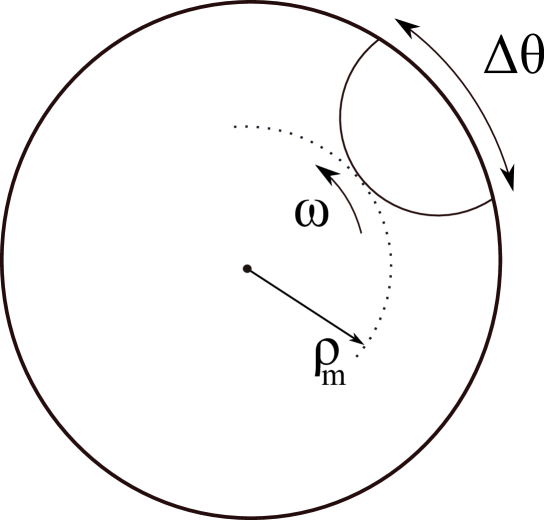
Figure 1: String ending on the boundary and rotating rigidly. The parameters that determine the solution are the angular velocity $\omega$ and the angular separation between the end points $\Delta\theta$. Alternatively one can use the angular velocity $\omega$ and the position $\rho_{m}$ of the point closest to the center.

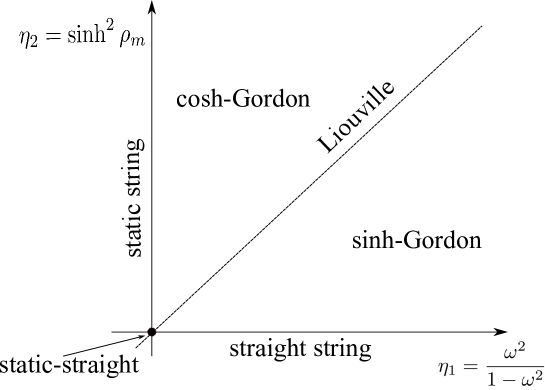
Figure 2: Depending on the relation between the angular velocity $\omega$ and the position of the lowest point of the string $\rho_{m}$, the equation obeyed by the world-sheet conformal factor is cosh-Gordon, Liouville or sinh-Gordon. The horizontal axis corresponds to a straight string ($\rho_{m}=0$) and the vertical one to a static string ($\omega=0$).

3 The general case

In the previous section, a rigidly rotating string demonstrated that the conformal factor can obey the cosh-Gordon, Liouville, or sinh-Gordon equations. Now, we consider the general, non-rigid, case. It is convenient to use embedding coordinates,

$$X_{1}^{2}+X_{2}^{2}-X_{3}^{2}-X_{4}^{2}=1,$$ (24)

and arrange them in a $2\times 2$ real matrix

$$\mathbb{X}=\left(\begin{array}[]{cc}X_{1}+X_{3}&X_{4}+X_{2}\\ X_{4}-X_{2}&X_{1}-X_{3}\end{array}\right)\,.$$ (25)

This matrix obeys $\det\mathbb{X}=1$, i.e. $\mathbb{X}\in SL(2,\mathbb{R})$. Consider the decomposition

$$\mathbb{X}=A_{1}A_{2}^{-1}\,,$$ (26)

with $\det A_{a}=1$, $a=1,2$. There is now a redundancy in the description and, as a result, a gauge symmetry

$$A_{a}\rightarrow A_{a}\,\mathcal{U}(\tau_{+},\tau_{-})\,,$$ (27)

leaves $\mathbb{X}$ invariant. Define now two one-forms:

$$J_{a}=A_{a}^{-1}dA_{a},\ \ \ a=1,2\,.$$ (28)

It follows, with no summation on $a$ implied, that

$$\mbox{Tr}J_{a}=0,\ \ \ dJ_{a}+J_{a}\wedge J_{a}=0.$$ (29)

To be precise, the conventions used for differential forms in coordinates $\tau_{\pm}=\tau\pm\sigma$ are:

$$a = a_{+}d\tau_{+}+a_{-}d\tau_{-},$$ (30)

$$da = (\partial_{-}a_{+}-\partial_{+}a_{-})\,d\tau_{-}\wedge d\tau_{+},$$ (31)

$$a\wedge b = (a_{-}b_{+}-a_{+}b_{-})d\tau_{-}\wedge d\tau_{+},$$ (32)

$$(*a)_{+}=a_{+},\ (*a)_{-}=-a_{-},\ \ *a\wedge b=-a\wedge*b,\ \ \ **a=a.$$ (33)

The equations of motion (3) become

$$*d\!*\!d\mathbb{X}=2\Lambda\,\mathbb{X}.$$ (34)

Expanding the derivatives in terms of the currents yields:

$$J_{1}\wedge*J_{1}+*J_{1}\wedge J_{2}-J_{1}\wedge*J_{2}-*J_{2}\wedge J_{2}+d*J_{1}-d*J_{2}=2\Lambda.$$ (35)

Since the currents are two by two traceless matrices the traceless part can be extracted by using commutators; namely,

$$A\wedge B\xrightarrow{\mbox{traceless part}}\frac{1}{2}(A\wedge B+B\wedge A).$$ (36)

Here, the right-hand side is the traceless part of the left-hand side. Thus, we get a simple equation

$$d*(J_{1}-J_{2})+*J_{1}\wedge J_{2}+J_{2}\wedge*J_{1}=0.$$ (37)

Also, the equations of motion can be written in terms of the currents:

$$dJ_{1}+J_{1}\wedge J_{1} = 0,$$ (38)

$$dJ_{2}+J_{2}\wedge J_{2} = 0,$$ (39)

$$d*(J_{1}-J_{2})+*J_{1}\wedge J_{2}+J_{2}\wedge*J_{1} = 0.$$ (40)

These equations need to be supplemented with the constraints $\det(\partial_{+}\mathbb{X})=0=\det(\partial_{-}\mathbb{X})$; equivalently,

$$\det(J_{1+}-J_{2+})=0=\det(J_{1-}-J_{2-}).$$ (41)

At this point, it is convenient to define two new currents,

$${\cal A}=\frac{1}{2}(J_{1}-J_{2}),\ \ \ {\cal B}=\frac{1}{2}(J_{1}+J_{2})\ ,$$ (42)

in terms of which the equations of motion can be rewritten:

$$d{\cal A}+{\cal A}\wedge{\cal B}+{\cal B}\wedge{\cal A} = 0,$$ (43)

$$d(*{\cal A})+(*{\cal A})\wedge{\cal B}+{\cal B}\wedge(*{\cal A}) = 0,$$ (44)

$$d{\cal B}+{\cal B}\wedge{\cal B}+{\cal A}\wedge{\cal A} = 0,$$ (45)

$$\det({\cal A}_{+})=\det({\cal A}_{-}) = 0,$$ (46)

$$\mbox{Tr}{\cal A}=\mbox{Tr}{\cal B} = 0.$$ (47)

A flat current can be found as a linear combination:

$$a = \alpha{\cal A}+\beta*\!{\cal A}+\gamma{\cal B},$$ (48)

$$da+a\wedge a = 0,$$ (49)

which in addition satisfies

$$\mbox{Tr}(a)=0.$$ (50)

There is a one parameter family of non-trivial solutions given by $(\alpha+\beta)(\alpha-\beta)=1$, $\gamma=1$. It can be conveniently parameterized in terms of the spectral parameter $\lambda$ as $\alpha+\beta=\lambda$, $\alpha-\beta=\frac{1}{\lambda}$. Thus:

$$a_{+} = \lambda{\cal A}_{+}+{\cal B}_{+},$$ (51)

$$a_{-} = \frac{1}{\lambda}{\cal A}_{-}+{\cal B}_{-}.$$ (52)

Since ${\cal A}$ and ${\cal B}$ are real but $\lambda$ is generically complex, the flat current $a$ satisfies the reality condition

$$\overline{a(\lambda)}=a(\bar{\lambda}).$$ (53)

It is also useful to note that $J_{1}=a(1)$, $J_{2}=a(-1)$. Returning to the current ${\cal A}$, and expanding it in terms of the Pauli matrices $\sigma_{a=1,2,3}$:

$${\cal A}_{+} = n_{1}\sigma_{1}+n_{2}i\sigma_{2}+n_{3}\sigma_{3},$$ (54)

$${\cal A}_{-} = \tilde{n}_{1}\sigma_{1}+\tilde{n}_{2}i\sigma_{2}+\tilde{n}_{3}\sigma_{3},$$ (55)

the condition $\det{\cal A}_{\pm}=0$ implies that $n$, $\tilde{n}$ are light-like vectors, i.e.

$$n_{2}^{2}-n_{1}^{2}-n_{3}^{2}=0,$$ (56)

and the same for $\tilde{n}$. The gauge symmetry $A_{a}\rightarrow A_{a}\,\mathcal{U}(\tau_{+},\tau_{-})$, in terms of ${\cal A}$, gives ${\cal A}_{a}\rightarrow\mathcal{U}(\tau_{+},\tau_{-})^{-1}{\cal A}_{a}\,\mathcal{U}(\tau_{+},\tau_{-})$ which is an $SL(2,\mathbb{R})=SO(2,1)$ rotation of the vectors $n$, $\tilde{n}$. Assuming that $n\neq\tilde{n}$, they can always be put in the form:

$$n=e^{\alpha}(1,1,0),\ \ \tilde{n}=e^{\alpha}(-1,1,0),$$ (57)

where $\alpha(\tau_{+},\tau_{-})$ is a real function. In this way, the current is

$${\cal A}=e^{\alpha}(d\tau_{+}\sigma_{+}+d\tau_{-}\sigma_{-}),$$ (58)

where $\sigma_{+}=\left(\begin{array}[]{cc}0&1\\ 0&0\end{array}\right)$, $\sigma_{-}=\left(\begin{array}[]{cc}0&0\\ 1&0\end{array}\right)$. The equation for ${\cal B}$ determines that

$${\cal B}_{+} = \frac{1}{2}\partial_{+}\,\alpha\,\sigma_{3}+u(\tau_{+})e^{-\alpha}\,\sigma_{-},$$ (59)

$${\cal B}_{-} = -\frac{1}{2}\partial_{-}\,\alpha\,\sigma_{3}+v(\tau_{-})e^{-\alpha}\,\sigma_{-},$$ (60)

where $u(\tau_{+})$ and $v(\tau_{-})$ are arbitrary functions and, in addition, $\alpha$ satisfies

$$\frac{1}{2}\partial_{+-}\alpha=e^{2\alpha}-e^{-2\alpha}u(\tau_{+})v(\tau_{-}).$$ (61)

By an appropriate change of coordinates $\tau_{\pm}$ and a redefinition of $\alpha$, one can set $u$ and $v$ to a constant except at those points where they vanish. In the rest of the paper we consider only the case where $uv$ is constant everywhere and can therefore be set equal to either, $-1$, $0$ or $+1$. The case where $uv$ vanishes at a finite set of points will not be considered since we do not know how to write the general solution in those cases.

The flat connection can be written as

$$a_{+}=\left(\begin{array}[]{cc}\frac{1}{2}\partial_{+}\alpha&\lambda e^{\alpha}\\ ue^{-\alpha}&-\frac{1}{2}\partial_{+}\alpha\end{array}\right),\ \ \ a_{-}=\left(\begin{array}[]{cc}-\frac{1}{2}\partial_{-}\alpha&ve^{-\alpha}\\ \frac{1}{\lambda}e^{\alpha}&\frac{1}{2}\partial_{-}\alpha\end{array}\right),$$ (62)

which is valid in general even if only the case of constant $u,v$ is considered here. Since $a$ is flat, we can solve the linear problem

$$d\Psi(\lambda;\tau_{+},\tau_{-})=\Psi(\lambda;\tau_{+},\tau_{-})a.$$ (63)

Moreover, since $J_{1}=a(1)$, $J_{2}=a(-1)$, we have $A_{1}=\Psi(1)$, $A_{2}=\Psi(-1)$; namely,

$$\mathbb{X}=\Psi(1)\Psi(-1)^{-1}.$$ (64)

Therefore, the strategy is to solve the equation for $\alpha$, replace it in the flat current, solve the linear problem, and reconstruct the solution $\mathbb{X}$. In fact, a family of solutions satisfying the equations of motion and the constraints can be introduced:

$$\mathbb{X}(\lambda)=\Psi(\lambda)\Psi(-\lambda)^{-1}.$$ (65)

Furthermore, the reality condition is satisfied if $\lambda\in\mathbb{R}$.

4 Liouville case ($uv=0$)

When $uv=0$, equation (61) reduces to the Liouville equation:

$$\frac{1}{2}\partial_{+-}\alpha=e^{2\alpha}.$$ (66)

The general solution to this equation is

$$\alpha=\frac{1}{2}\ln\left(\frac{2\partial_{+}f(\tau_{+})\partial_{-}\tilde{f}(\tau_{-})}{(1-f(\tau_{+})\tilde{f}(\tau_{-}))^{2}}\right).$$ (67)

In this case, to reconstruct the solution $X_{\mu}(\tau_{+},\tau_{-})$, we can side-step the procedure described in the previous section and directly solve the linear problem

$$\partial_{+-}X^{\mu}=e^{2\alpha}X^{\mu}.$$ (68)

Using separation of variables (and taking as coordinates $f,\tilde{f}$) or by any other technique, the general solution is found to be

$$X^{\mu}=\left[\frac{1+f\tilde{f}}{1-f\tilde{f}}h^{\mu}_{+}(\tau_{+})+\frac{f}{\partial_{+}f}\partial_{+}h_{+}^{\mu}(\tau_{+})\right]+\left[\frac{1+f\tilde{f}}{1-f\tilde{f}}h^{\mu}_{-}(\tau_{-})+\frac{\tilde{f}}{\partial_{-}\tilde{f}}\partial_{-}h_{-}^{\mu}(\tau_{-})\right].$$ (69)

where $h^{\mu}_{+}(\tau_{+})$ and $h^{\mu}_{-}(\tau_{-})$ are arbitrary functions. Although this satisfies the equations of motion, it also needs to satisfy the constraints

$$(\partial_{+}X^{\mu})^{2}=0=(\partial_{-}X^{\mu})^{2},\ \ \ X^{2}=1.$$ (70)

Although particular solutions exist, it appears that generic solutions cannot be found in the case where both $h_{+}$ and $h_{-}$ are different from zero. In this paper, only the case where $h^{\mu}_{-}=0$ is considered and the solution is

$$X^{\mu}=\left[\frac{1+f\tilde{f}}{1-f\tilde{f}}h^{\mu}_{+}(\tau_{+})+\frac{f}{\partial_{+}f}\partial_{+}h_{+}^{\mu}(\tau_{+})\right].$$ (71)

The constraints then reduce to

$$h^{2} = 0,$$ (72)

$$(\partial_{+}h)^{2} = (\partial_{+}\ln f)^{2},$$ (73)

$$(\partial_{++}h)^{2} = (\partial_{++}\ln f)^{2}-(\partial_{+}\ln f)^{4}.$$ (74)

These are relatively easy to study by noting that different choices of the functions $f(\tau_{+})$, $\tilde{f}(\tau_{-})$ are related by reparameterizations of the world-sheet and, therefore, equivalent. In this way, we can choose for example

$$f=e^{i\tau_{+}},\ \ \tilde{f}=-e^{i\tau_{-}},$$ (75)

without loosing generality. Now, the solution can be written as

$$X^{\mu}=\tan\sigma\ h_{+}^{\mu}(\tau_{+})+\partial_{+}h_{+}^{\mu},$$ (76)

with

$$h_{+}^{2}=0,\ \ (\partial_{+}h_{+})^{2}=1,\ \ \ (\partial_{++}h_{+})^{2}=1.$$ (77)

The string ends at the boundary on two curves determined by $\sigma=\pm\frac{\pi}{2}$. The curves are given by

$$X^{\mu}=\pm h^{\mu}_{+}(\tau\pm\frac{\pi}{2}).$$ (78)

Notice that $X^{2}=0$ which is a parameterization of the boundary of ${AdS}$ space. Furthermore, these solutions are valid for any ${AdS}$ and not only ${AdS}_{3}$. In fact they are already known since they were found by Mikhailov in [5]. In particular, they contain the solution corresponding to the rotating string described in the first section. To show that, start by parameterizing the boundary curves as

$$h_{+}^{\mu}=\left(\begin{array}[]{c}\cos t\\ \sin t\\ \sin\theta\\ \cos\theta\end{array}\right).$$ (79)

Next, observe that, according to eq.(78), the two boundary curves are the same up to a shift by $\pi$ in the parameter $\tau$ and a change in sign of $h_{+}^{\mu}$, which is equivalent to a shift $t\rightarrow t+\pi,$ , $\theta\rightarrow\pi+\theta$. Since the shift in parameter $\tau$ does not change the shape of the curve, one curve is obtained from the other by rotating $\theta$ by $\pi$ and shifting $t$ also by $\pi$. Therefore, the shape of one boundary curve can be chosen arbitrarily, which determines the functions $h^{\mu}_{+}(\tau_{+})$ and also the shape of the other boundary curve.

For the rigidly rotating string, we have that one curve is determined by

$$\theta_{1}=\omega t.$$ (80)

Consequently, the other is

$$\theta_{2}+\pi=\omega(t+\pi),$$ (81)

This implies that

$$\Delta\theta=\theta_{1}-\theta_{2}=\pi(1-\omega),$$ (82)

which is precisely the result in eq.(16). Physically, this means that a ray of light emitted from the quark reaches the anti-quark exactly after a time $t=\pi$. If it reaches earlier or later we then have the cosh or sinh Gordon equation. In Poincare coordinates, the two end points of the string describe arbitrary trajectories that are asymptotically null. In this case, it should be noted that both trajectories are arbitrary since they come from different portions of the trajectory in global ${AdS}_{.}$ The only condition is that one asymptotes to a null direction that is equal to the incoming direction of the other one. See fig.3.

Figure 3: In Poincare coordinates, the Liouville case generically corresponds to a string ending on two arbitrary paths which are asymptotically light-like. The only condition is that the outgoing direction of one of them is equal to the incoming direction of the other one.

5 Sinh/cosh Gordon case ($uv=\pm 1$)

The other case to consider is when the world-sheet conformal factor obeys the sinh or cosh-Gordon equation, i.e. eq.(61) with $uv=\pm 1$. The solution can be written in terms of theta functions associated with a hyperelliptic Riemann surface. The reality condition implies that the Riemann surface can be thought as two planes connected by a set of cuts symmetric under the interchange $\lambda\leftrightarrow\bar{\lambda}$. In the examples considered here, the cuts are on the real axis although other situations are possible.

To be concrete, the hyperelliptic Riemann surface of genus $g$ is defined by the equation

$$\mu^{2}=\prod_{i=1}^{2g+1}(\lambda-\lambda_{i}),$$ (83)

where $(\mu,\lambda)$ parameterize $\mathbb{C}^{2}$. A basis of 1-cycles $(a_{i},b_{i})$ is chosen together with a basis of normalized holomorphic differentials $\omega$. Points on the Riemann surface are denoted as $p_{i}$ whereas their projection on the complex plane is denoted as $\lambda_{p_{i}}$. Obviously, each $\lambda_{p_{i}}$ corresponds to two points on the Riemann surface (upper and lower sheets) except for the branch points $\lambda_{i}$. Two of the branch points are going to be singled out and denoted as $p_{1}$ and $p_{3}$. Take a path from $p_{1}$ to $p_{3}$ on the upper sheet and close it by tracing the same path backwards on the lower sheet. When written in the basis $(a_{i},b_{i})$, the closed path $\mathcal{C}_{13}$ defines two integer vectors $\Delta_{1}$ and $\Delta_{2}$ such that

$$\mathcal{C}_{13}=\Delta_{2i}a_{i}+\Delta_{1i}b_{i}\,.$$ (84)

These vectors, together with the periodicity matrix of the Riemann surface, define a theta function with characteristics:

$$\hat{\theta}(\zeta)=\theta\left[\begin{array}[]{c}\Delta_{1}\\ \Delta_{2}\end{array}\right](\zeta),\ \ \ \ \zeta\in\mathbb{C}^{g}$$ (85)

This function and the usual theta function $\theta(\zeta)$ without characteristics determine a function $\alpha(\tau_{+},\tau_{-})$

$$e^{\alpha}=C_{\alpha}\frac{\theta(\zeta)}{\hat{\theta}(\zeta)},\ \ \ \ \ \zeta=C_{-}\,\hat{\omega}_{1}\,\tau_{-}+C_{+}\,\hat{\omega}_{3}\,\tau_{+}$$ (86)

which solves the sinh/cosh-Gordon equation. The constant $C_{\alpha}$ is such that $C_{\alpha}^{4}=1$ and should be chosen such that the right hand side is real and positive. This is always possible since the reality conditions ensure that $\theta(\zeta)$ is real and $\hat{\theta}(\zeta)$ is either real or purely imaginary. Moreover, as discussed later, this is the only reality condition needed. As explained below, once $\alpha$ is real, a real solution for $X^{\mu}(\sigma,\tau)$ can always be obtained. More details on the notation and derivations can be found in the appendix including the definition of the vectors $\hat{\omega}_{1,3}$. Finally, the constants $C_{\pm}$ are such that $C_{\pm}^{2}=1$ and should be chosen such that

$$C_{+}C_{-}=e^{i\pi\Delta_{2}^{t}\Delta_{1}}\,C_{\alpha}^{2}.$$ (87)

With these definitions, it is just a matter of algebra to check that $\alpha$ satisfies the equation

$$\partial_{+-}\alpha=e^{2\alpha}-e^{i\pi\Delta_{2}^{t}\Delta_{1}}e^{-2\alpha},$$ (88)

as shown in the appendix. Consequently, we have to identify

$$uv=e^{i\pi\Delta_{1}^{t}\Delta_{2}}.$$ (89)

In what follows, it is convenient to choose

$$u=1,v=e^{i\pi\Delta_{1}^{t}\Delta_{2}}=\pm 1$$ (90)

Summarizing, if we choose $\lambda_{p_{1}}$, $\lambda_{p_{3}}$ such that $\Delta_{2}^{t}\Delta_{1}$ is even, we have the sinh-Gordon equation. If we choose them such that $\Delta_{2}^{t}\Delta_{1}$ is odd we obtain the cosh-Gordon one.

It should be noted that there is a different solution

$$e^{\alpha}=C_{\alpha}\frac{\theta(i\zeta)}{\hat{\theta}(i\zeta)},$$ (91)

which is interesting but simply related by $\zeta\rightarrow i\zeta$ to the previous one. For that reason it is not considered further.

The next step is to write the flat current $a(\lambda)$ and find the matrix $\Psi$ that satisfies

$$d\Psi(\lambda)=a(\lambda)\Psi(\lambda).$$ (92)

The matrix $\Psi$ is a two by two matrix that we write as

$$\Psi=\left(\begin{array}[]{cc}\psi_{1}&\psi_{2}\\ \tilde{\psi}_{1}&\tilde{\psi}_{2}\end{array}\right),$$ (93)

where $(\psi_{1},\psi_{2})$ and $(\tilde{\psi}_{1},\tilde{\psi}_{2})$ are two linearly independent solutions of the equation

$$d\psi(\lambda)=a(\lambda)\psi(\lambda),$$ (94)

where $\psi$ is now a two dimensional row vector. Using expression (62) for $a(\lambda)$, the equations can be rewritten:

$$\partial_{+}\psi_{1} = \frac{1}{2}\partial_{+}\alpha\psi_{1}+ue^{-\alpha}\psi_{2},$$ (95)

$$\partial_{+}\psi_{2} = \lambda e^{\alpha}\psi_{1}-\frac{1}{2}\partial_{+}\alpha\psi_{2},$$ (96)

$$\partial_{-}\psi_{1} = -\frac{1}{2}\partial_{-}\alpha\psi_{1}+\frac{1}{\lambda}e^{\alpha}\psi_{2},$$ (97)

$$\partial_{-}\psi_{2} = ve^{-\alpha}\psi_{1}+\frac{1}{2}\partial_{-}\alpha\psi_{2}.$$ (98)

Here $u$ and $v$ are as in eq.(90). It is important to note that once $\alpha$ is real and the spectral parameter $\lambda$ is taken real, $\psi_{1,2}$ obey real equations and, therefore, can always be taken to be real. For example, given a solution, its real and imaginary part are real and also solve the equations.

Now we can proceed to solve the equations. One way to do it is to convert them into an equation for the ratio $\psi_{1}/\psi_{2}$ which can then be solved using the identities (158). Afterwards, one can solve for $\psi_{1,2}$ individually, again using eqns.(158). The result is

$$\psi_{1} = C_{1}e^{\frac{1}{2}\alpha}\frac{\theta(\zeta+\int_{1}^{4})}{\theta(\zeta)}\ e^{\mu_{+}\sigma_{+}+\mu_{-}\sigma_{-}},$$ (99)

$$\psi_{2} = C_{2}e^{\frac{1}{2}\alpha}\frac{\theta(a+\int_{4}^{1})}{\hat{\theta}(a+\int_{4}^{1})}\frac{\hat{\theta}(\zeta+\int_{1}^{4})}{\theta(\zeta)}\ e^{\mu_{+}\sigma_{+}+\mu_{-}\sigma_{-}},$$ (100)

where the constants $C_{1,2}$, $\mu_{\pm}$ and $\lambda$ need to be determined. By comparing with the theta function identities found in the appendix, eq.(158), one finds that the spectral parameter is given by

$$\lambda(\lambda_{p_{4}})=C_{\lambda}\,\frac{\theta^{2}(a+\int_{4}^{1})}{\hat{\theta}^{2}(a+\int_{4}^{1})}=A_{0}\frac{\lambda_{p_{4}}-\lambda_{p_{1}}}{\lambda_{p_{4}}-\lambda_{p_{3}}}\ .$$ (101)

That the ratio of theta functions simplifies as in the last equation is explained in the appendix. Here $A_{0}$ is a constant independent of $\lambda_{p_{4}}$ but dependent on the other parameters of the solution; namely, the Riemann surface and the points $\lambda_{p_{1}}$, $\lambda_{p_{3}}$. The other constants are such that

$$C_{\lambda}=v,\ \ \ C_{2}=C_{\alpha}C_{+}C_{1}.$$ (102)

The constants $\mu_{\pm}$ turn out to be

$$\mu_{+} = -C_{+}\frac{\hat{\theta}(a)}{D_{3}\theta(a)}D_{3}\ln\frac{\hat{\theta}(a)}{\hat{\theta}(a+\int_{4}^{1})},$$ (103)

$$\mu_{-} = -C_{-}\frac{\hat{\theta}(a)}{D_{1}\theta(a)}D_{1}\ln\frac{\hat{\theta}(a)}{{\theta}(a+\int_{4}^{1})}.$$ (104)

As discussed in the appendix, there are three possible cases:

• $v=+1$, $\theta,\hat{\theta}$ are real. The equation is sinh-Gordon and we can take $C_{+}=C_{-}=C_{\lambda}=1$ and $C_{\alpha}=\pm 1$ such that $e^{\alpha}>0$. Finally $C_{2}=C_{\alpha}C_{1}$.

• $v=-1$, $\theta,\hat{\theta}$ are real. The equation is cosh-Gordon and we can take $C_{+}=1$, $C_{-}=C_{\lambda}=-1$ and $C_{\alpha}=\pm 1$ such that $e^{\alpha}>0$. Finally $C_{2}=C_{\alpha}C_{1}$.

• $v=-1$, $\theta$ real,$\hat{\theta}$ purely imaginary. The equation is cosh-Gordon and we can take $C_{+}=C_{-}=1$, $C_{\lambda}=-1$ and $C_{\alpha}=\pm i$ such that $e^{\alpha}>0$. Finally $C_{2}=C_{\alpha}C_{1}$.

As discussed above, $\psi_{1,2}$ obey real equations; therefore, if the previous solutions are complex, in fact, two solutions are obtained and are given by its real and imaginary part. If those are independent we are done. Otherwise, we have to find another linearly independent solution which can be easily done:

$$\tilde{\psi}_{1} = Ae^{\frac{1}{2}\alpha}\frac{\theta(\zeta+\int_{1}^{\bar{4}})}{\theta(\zeta)}\ e^{\tilde{\mu}_{+}\sigma_{+}+\tilde{\mu}_{-}\sigma_{-}},$$ (105)

$$\tilde{\psi}_{2} = Ae^{\frac{1}{2}\alpha}\frac{\theta(a+\int_{\bar{4}}^{1})}{\hat{\theta}(a+\int_{\bar{4}}^{1})}\frac{\hat{\theta}(\zeta+\int_{1}^{\bar{4}})}{\theta(\zeta)}\ e^{\tilde{\mu}_{+}\sigma_{+}+\tilde{\mu}_{-}\sigma_{-}}.$$ (106)

The notation $\bar{4}$ denotes the point $\bar{p}_{4}$ which is different from $p_{4}$ but has the same projection $\lambda_{p_{4}}$. That is, one is in the lower sheet and the other in the upper sheet. Notice that in eq.(101), the value of $\lambda$ depends only on $\lambda_{p_{4}}$ meaning that it does not matter if $p_{4}$ is in the upper or lower sheet; therefore, $(\psi_{1},\psi_{2})$ and $(\tilde{\psi}_{1},\tilde{\psi}_{2})$ satisfy the same differential equation. Furthermore, define the constants $\tilde{\mu}_{\pm}$ by replacing $4\rightarrow\bar{4}$.

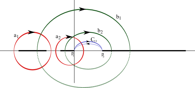
Figure 4: A simple example of Riemann surface with three cuts ($g=2$) and a choice of basis $(a_{i},b_{i})$ for the cycles. The cuts are on the real axis implying symmetry under $\lambda\leftrightarrow\bar{\lambda}$. Furthermore, under conjugation, $\bar{a}_{i}=-a_{i}$, $\bar{b}_{i}=b_{i}$. Two of the branch points are chosen as $p_{1}$ and $p_{3}$. They define the path $C_{13}$ which in this case is just $C_{13}=b_{2}$. Therefore, in this example, $\Delta_{1}=[0,1]$ and $\Delta_{2}=[0,0]$.

In this way, we have found $\Psi(\lambda)$. However, we know that the solution is given by $\mathbb{X}=\Psi(\lambda)\Psi(-\lambda)^{-1}$ so we still need to find $\Psi(-\lambda)$. Since $\Psi(-\lambda)$ satisfies the same equation, the solution is similar, we only need to find a point $\lambda_{p_{4^{\prime}}}$ such that

$$\lambda^{\prime}=C_{\lambda}\,\frac{\theta^{2}(a+\int_{4}^{1})}{\hat{\theta}^{2}(a+\int_{4}^{1})}=-\lambda.$$ (107)

Given the formula

$$C_{\lambda}\,\frac{\theta^{2}(a+\int_{4}^{1})}{\hat{\theta}^{2}(a+\int_{4}^{1})}=A_{0}\frac{\lambda_{p_{4}}-\lambda_{p_{1}}}{\lambda_{p_{4}}-\lambda_{p_{3}}},$$ (108)

such point is simply given by

$$\lambda_{p_{4^{\prime}}}=\frac{\lambda_{p_{4}}(\lambda_{p_{1}}+\lambda_{p_{3}})-2\lambda_{p_{1}}\lambda_{p_{3}}}{2\lambda_{p_{4}}-\lambda_{p_{1}}-\lambda_{p_{3}}}.$$ (109)

Replacing $\lambda_{p_{4}}$ by $\lambda_{p_{4^{\prime}}}$ everywhere, we find $\Psi(-\lambda)$ and with that the solution $\mathbb{X}(\tau_{+},\tau_{-})$. In fact, a family of solutions parameterized by a real parameter $\lambda$ (or equivalently the point $p_{4}$). Having taken care of choosing real solutions for $\Psi(\pm\lambda)$, the solution $\mathbb{X}$ is real. The constraints are also automatically satisfied by construction. The best way of understanding what type of solutions these represent is, perhaps, to work out an example as we do in the next section.

6 Examples

To get an idea of the shape of the solutions, we give here two examples, one corresponds to the sinh-Gordon and the other to the cosh-Gordon case. We give (approximate) numerical values for all the quantities appearing in the solution so that the interested reader can reproduce the results if he/she so desires. For simplicity, the auxiliary Riemann surface is taken to be of genus $g=2$. The cuts are taken on the real axis as $[-2,-1]$, $[-\frac{1}{2},0]$ and $[1,\infty]$. The point $p_{1}$ is taken as $p_{1}=0$ and the point $p_{3}$ is $p_{3}=1$ for the sinh-Gordon case and $p_{3}=-1$ for the cosh-Gordon case. The cycles $a_{1,2}$ and $b_{1,2}$ are taken as in fig.4 which determines (see the appendix for details on the procedure)

$$C_{ij} = \oint_{a_{i}}\frac{\lambda^{i-1}}{\mu(\lambda)}\ d\lambda=\left(\begin{array}[]{cc}3.691&-5.042\\ -5.042&1.351\end{array}\right)_{ij}\ \ ,$$ (112)

$$\tilde{C}_{ij} = \oint_{b_{i}}\frac{\lambda^{i-1}}{\mu(\lambda)}\ d\lambda=\left(\begin{array}[]{cc}1.351i&-5.042i\\ -3.691i&-1.351i\end{array}\right)_{ij}\ \ \ .$$ (115)

where

$$\mu^{2}(\lambda)=(\lambda+2)(\lambda+1)(\lambda+\frac{1}{2})\lambda(\lambda-1)$$ (116)

The periodicity matrix is given by

$$\Pi=\tilde{C}\,C^{-1}=\left(\begin{array}[]{cc}1.155i&0.577i\\ 0.577i&1.155i\end{array}\right).$$ (117)

The zero of the theta function $a$ is taken as the odd half period:

$$a=\frac{1}{2}\left[\begin{array}[]{c}0\\ 1\end{array}\right]+\frac{1}{2}\Pi\left[\begin{array}[]{c}0\\ 1\end{array}\right]=\left[\begin{array}[]{c}0.289i\\ \frac{1}{2}+0.577i\end{array}\right].$$ (118)

The normalized holomorphic differentials are

$$\omega_{i}=\frac{\lambda^{j-1}}{\mu(\lambda)}\,C^{-1}_{ji}\ \ \ \Rightarrow\ \ \ \oint_{a_{j}}\omega_{i}=\delta_{ij}.$$ (119)

Now we consider two separate examples: one for sinh and the other for cosh-Gordon.

6.1 Sinh-Gordon

For the sinh-Gordon case, we choose $p_{1}=0$, $p_{3}=1$ that determines the characteristic of $\hat{\theta}$ as:

$$\int_{p_{1}}^{p_{3}}\,\omega=\frac{1}{2}\Delta_{2}+\frac{1}{2}\Pi\Delta_{1}\ \ \ \Rightarrow\ \ \ \Delta_{1}=\left[\begin{array}[]{c}0\\ 1\end{array}\right],\ \ \ \Delta_{2}=\left[\begin{array}[]{c}0\\ 0\end{array}\right]$$ (120)

which is even and therefore leads to the sinh-Gordon equation. The constants are simply taken to be

$$C_{\alpha}=C_{1}=C_{2}=C_{+}=C_{-}=1.$$ (121)

The point $p_{4}$ is taken on the upper sheet such that $\lambda_{p_{4}}=0.23$ giving

$$\int_{1}^{4}\omega=\left[\begin{array}[]{c}0.0744i\\ 0.230i\end{array}\right],$$ (122)

and

$$\lambda=\lambda(\lambda_{p_{4}})=C_{\lambda}\,\frac{\theta^{2}(a+\int_{4}^{1})}{\hat{\theta}^{2}(a+\int_{4}^{1})}=-0.597$$ (123)

We can now write the vector $\zeta(\tau_{+},\tau_{-})$ that appears in the argument of the theta functions as (see eq.(86))

$$\zeta(\tau_{+},\tau_{-})=\left[\begin{array}[]{c}-0.295\\ -0.403\end{array}\right]\tau_{+}-\left[\begin{array}[]{c}0.0935\\ 0.349\end{array}\right]\tau_{-}$$ (124)

Finally, we need the constants

$$\mu_{+}=-\tilde{\mu}_{+}=0.307\,i,\ \ \ \ \mu_{-}=-\tilde{\mu}_{-}=-1.765\,i$$ (125)

This allows us to use eqn.(93) and write $\Psi(\lambda)$ as

$$\Psi(\lambda=-0.597)=\left(\begin{array}[]{cc}{\mathcal{R}e}\,\psi_{1}&{\mathcal{R}e}\,\psi_{2}\\ {\mathcal{I}m}\,\psi_{1}&{\mathcal{I}m}\,\psi_{2}\end{array}\right)$$ (126)

In this case, the solutions $(\psi_{1},\psi_{2})$ and $(\tilde{\psi}_{1},\tilde{\psi}_{2})$ are complex and conjugate to each other. Therefore, we only need the real and imaginary part of one of them to have two independent solutions. The overall normalization $\det\Psi=1$ can be easily fixed later since $\det\Psi$ is a constant independent of $\tau_{+},\tau_{-}$.

Finally, to construct $\mathbb{X}$, according to eq.(65), we also need to find $\Psi(-\lambda)$. For that purpose, choose a new point $p^{\prime}_{4}$ determined from equation eq.(170):

$$\lambda_{p_{4^{\prime}}}=-0.426\ .$$ (127)

We are going to denote with a prime all quantities associated to this new choice of $p_{4}$. We find

$$\int_{1}^{4^{\prime}}\omega=\left[\begin{array}[]{c}-0.0372\\ -0.383\end{array}\right]\ ,$$ (128)

and

$$\lambda^{\prime}=\lambda(\lambda_{p_{4^{\prime}}})=C_{\lambda}\,\frac{\theta^{2}(a+\int_{4^{\prime}}^{1})}{\hat{\theta}^{2}(a+\int_{4^{\prime}}^{1})}=.597\ ;$$ (129)

namely, indeed $\lambda^{\prime}=-\lambda$. Finally, we have the new constants

$$\mu^{\prime}_{+}=-\tilde{\mu}^{\prime}_{+}=-0.0868,\ \ \ \ \ \ \ \mu^{\prime}_{-}=-\tilde{\mu}^{\prime}_{-}=-0.425\ .$$ (130)

This allows us to put together $\Psi(\lambda^{\prime}=-\lambda)$ using eqns.(100) with the new values of the constants:

$$\Psi(\lambda^{\prime}=0.597)=\left(\begin{array}[]{cc}\psi^{\prime}_{1}&\psi^{\prime}_{2}\\ \tilde{\psi}^{\prime}_{1}&\tilde{\psi}^{\prime}_{2}\end{array}\right).$$ (131)

In this case, the solutions $(\psi^{\prime}_{1},\psi^{\prime}_{2})$ and $(\tilde{\psi}^{\prime}_{1},\tilde{\psi}^{\prime}_{2})$ are real and linearly independent; we use them in constructing $\Psi(\lambda^{\prime}=-\lambda)$. We now simply compute

$$\mathbb{X}=\Psi(\lambda)\Psi(-\lambda)^{-1},$$ (132)

up to a normalization to ensure that $\det\mathbb{X}=1$. Notice that from the equations, $\det\mathbb{X}$ is independent of $(\tau_{+},\tau_{-})$ so this is just an overall normalization. The solutions are plotted in fig.5. The coordinates used are global coordinates $(t,\theta,\rho)$:

$$t = \arctan\frac{\mathbb{X}_{11}+\mathbb{X}_{22}}{\mathbb{X}_{12}-\mathbb{X}_{21}},$$ (133)

$$\theta = \arctan\frac{\mathbb{X}_{11}-\mathbb{X}_{22}}{\mathbb{X}_{12}+\mathbb{X}_{21}},$$ (134)

$$\tanh^{2}\rho = \frac{\mbox{Tr}(\mathbb{X}\mathbb{X}^{t})-2\det\mathbb{X}}{\mbox{Tr}(\mathbb{X}\mathbb{X}^{t})-2\det\mathbb{X}}.$$ (135)

In the plots, for a better visualization, the coordinate $0<\tanh^{2}\rho<1$ was used instead of $\rho$. The horizontal plane $\tanh^{2}\rho=1$ is the boundary. It is interesting to note that, near the boundary, the world-sheet is almost light-like and one can wonder if the near speed of light expansion discussed in [29] may apply here. Although from the boundary point of view this is not clear, from the bulk point of view, the solutions discussed here and the solutions discussed in [6, 9] are essentially the same up to the reality conditions. In that sense an open string is somehow the analytic continuation of a closed string as already noted in [30]. We leave this as an interesting topic for further analysis and we discuss now an example for the cosh-Gordon case.

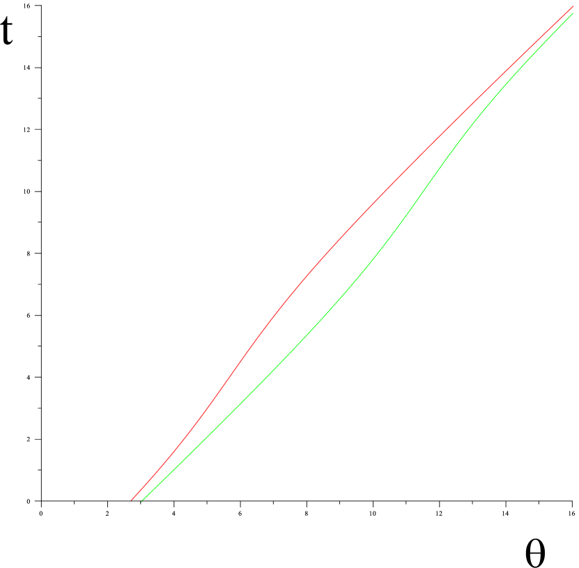
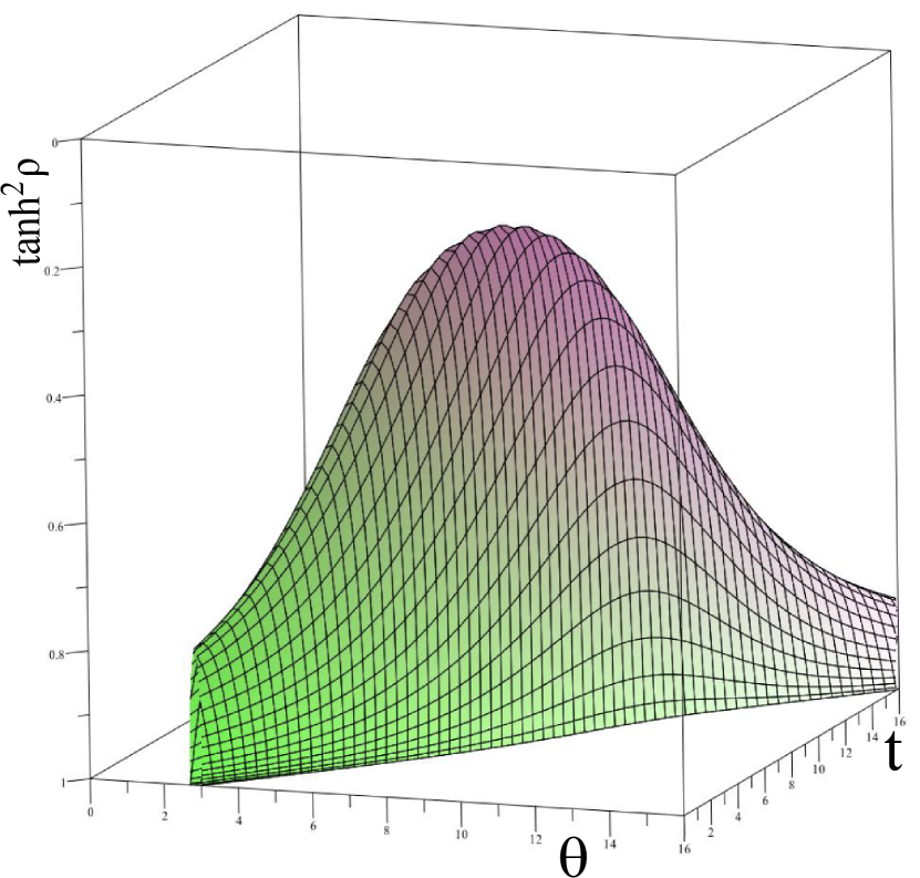
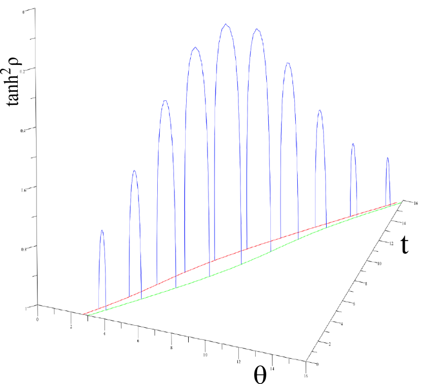
Figure 5: String ending on the boundary in global coordinates for the case of sinh-Gordon equation. The first picture displays the trajectories of the end points of the string in the boundary. The second and third one depicts the world-sheet in two different ways for clarity. The vertical axis is $\tanh^{2}\rho$. The bottom plane corresponds to $\rho=\infty$, i.e. $\tanh^{2}\rho=1$.

6.2 cosh-Gordon

A similar example can be used to illustrate the cosh-Gordon case. The calculations are completely similar so we just go briefly over them. In fact, we can take the same Riemann surface but choose $p_{1}=0$, $p_{3}=-1$ which determines the characteristic of $\hat{\theta}$ to be

$$\Delta_{1}=\left[\begin{array}[]{c}1\\ 1\end{array}\right],\ \ \ \Delta_{2}=\left[\begin{array}[]{c}0\\ 1\end{array}\right],$$ (136)

which is now odd and leads to the cosh-Gordon equation. The constants are

$$C_{\alpha}=-i,\ \ C_{+}=1,\ \ C_{-}=1,\ \ C_{1}=1,\ \ C_{2}=-i\ .$$ (137)

We choose again $\lambda_{p_{4}}=0.23$ although this time we obtain $p^{\prime}_{4}=-0.158$. This determines

$$\int_{1}^{4}\omega=\left[\begin{array}[]{c}0.0744i\\ 0.230i\end{array}\right],\ \ \ \ \int_{1}^{4^{\prime}}\omega=\left[\begin{array}[]{c}-0.0449\\ -0.203\end{array}\right],$$ (138)

and

$$\lambda=-\lambda^{\prime}=\lambda(\lambda_{p_{4}})=C_{\lambda}\,\frac{\theta^{2}(a+\int_{4}^{1})}{\hat{\theta}^{2}(a+\int_{4}^{1})}=-0.374\ .$$ (139)

The argument of the theta function is

$$\zeta(\tau_{+},\tau_{-})=\left[\begin{array}[]{c}-0.511i\\ 0.187i\end{array}\right]\tau_{+}-\left[\begin{array}[]{c}0.0935i\\ 0.349i\end{array}\right]\tau_{-}\ .$$ (140)

Finally, we compute the constants

$$\mu_{+}=-\tilde{\mu}_{+}=-0.246,\ \ \ \ \mu_{-}=-\tilde{\mu}_{-}=-1.765,$$ (141)

$$\mu^{\prime}_{+}=-\tilde{\mu}^{\prime}_{+}=-0.190\,i,\ \ \ \ \mu^{\prime}_{-}=-\tilde{\mu}^{\prime}_{-}=1.484\,i\ .$$ (142)

We reconstruct the solution

$$\Psi(\lambda=-0.374)=\left(\begin{array}[]{cc}\psi_{1}&\psi_{2}\\ \tilde{\psi}_{1}&\tilde{\psi}_{2}\end{array}\right),$$ (143)

$$\Psi(\lambda=0.374)=\left(\begin{array}[]{cc}{\mathcal{R}e}\,\psi^{\prime}_{1}&{\mathcal{R}e}\,\psi^{\prime}_{2}\\ {\mathcal{I}m}\,\tilde{\psi}^{\prime}_{1}&{\mathcal{I}m}\,\tilde{\psi}^{\prime}_{2}\end{array}\right).$$ (144)

The resulting $\mathbb{X}=\Psi(\lambda)\Psi^{-1}(-\lambda)$ is plotted in fig.6.

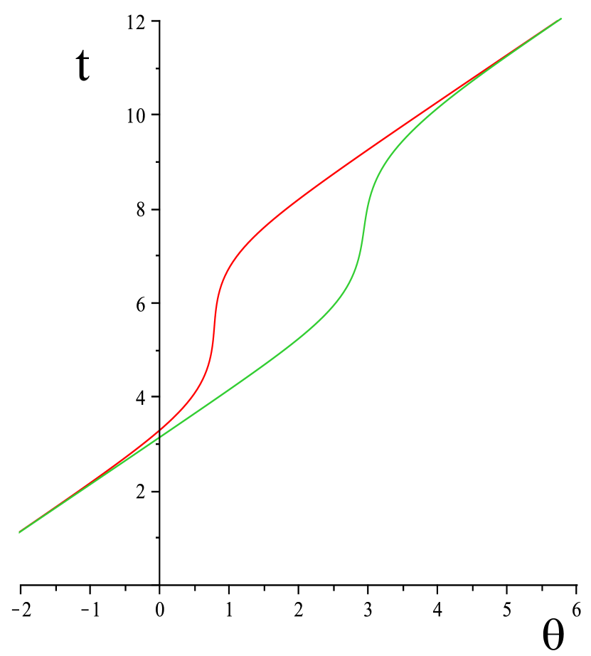
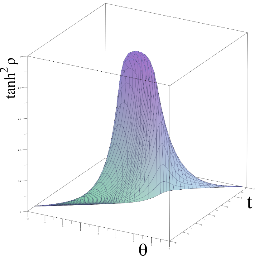
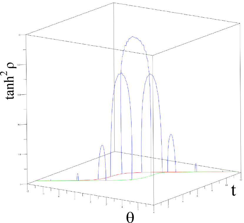
Figure 6: String ending on the boundary in global coordinates for the case of cosh-Gordon equation. The first picture displays the trajectories of the end points of the string in the boundary. The second and third one depicts the world-sheet in two different ways for clarity. The vertical axis is $\tanh^{2}\rho$. The bottom plane corresponds to $\rho=\infty$, i.e. $\tanh^{2}\rho=1$.

7 Acknowledgments

We are grateful to Peter Ouyang for discussions and to A. Tseytlin for a discussion that lead to this paper and also comments on the final version. This work was supported in part by NSF through grants PHY-0805948, a CAREER Award PHY-0952630, by DOE through grant DE-FG02-91ER40681 and by the SLOAN Foundation. In addition, M.K. is grateful to Perimeter Institute and M.K. and A.I. to the Simons Center for Geometry and Physics for hospitality while part of this work was being done.

Appendix A Theta function identities

Given a symmetric matrix $\Pi\in\mathbb{C}^{g\times g}$ with positive definite imaginary part, the theta function is defined as

$$\theta(\zeta)=\sum_{n\in\mathbb{Z}^{g}}e^{i\pi n^{t}\Pi n+2\pi in^{t}\zeta},\ \ \ \ \ \zeta\in\mathbb{C}^{g}\ ,$$ (145)

We also need another theta function defined as

$$\hat{\theta}(\zeta) = \theta\left[\begin{array}[]{c}\Delta_{1}\\ \Delta_{2}\end{array}\right]$$

$$= \exp\left\{2\pi i\left[\frac{1}{8}\Delta_{1}^{t}\Pi\Delta_{1}+\frac{1}{2}\Delta_{1}^{t}\zeta+\frac{1}{4}\Delta_{1}^{t}\Delta_{2}\right]\right\}\theta\left(\zeta+\frac{1}{2}\Delta_{2}+\frac{1}{2}\Pi\Delta_{1}\right)\ ,$$

where $\Delta_{1,2}$ are vectors whose components are either zero or one. It is important to notice if $\Delta_{1}^{t}\Delta_{2}$ is even or odd since that determines the parity of $\hat{\theta}$:

$$\hat{\theta}(-\zeta)=e^{i\pi\Delta_{1}^{t}\Delta_{2}}\hat{\theta}(\zeta).$$ (149)

Although the matrix $\Pi$ is an arbitrary complex matrix (up to the above mentioned conditions), when it is taken to be the period matrix of a hyperelliptic Riemann surface, the corresponding theta function has special properties. To be precise, consider the Riemann surface defined as a subspace of $\mathbb{C}^{2}$ (parameterized by $(\mu,\lambda)$ ) by the equation

$$\mu^{2}=\prod_{i=1}^{2g+1}(\lambda-\lambda_{i}).$$ (150)

As discussed in section 5 below eq.(83), points on the Riemann surface are denoted as $p_{i}$ whereas their projection is $\lambda_{p_{i}}$. Define a basis of cycles $(a_{i},b_{i})$ and consider the differentials

$$\nu_{i}=\frac{\lambda^{i-1}}{\mu}d\lambda,\ \ \ \ i=1\cdots g\ .$$ (151)

The index is restricted to $i=1\cdots g$ so that the differential is regular at zero and infinity. We compute the $g\times g$ complex matrices

$$C_{ij}=\oint_{a_{i}}\nu_{j},\ \ \ \ \tilde{C}_{ij}=\oint_{b_{i}}\nu_{j},$$ (152)

which allows to choose a basis of normalized holomorphic differentials $\omega_{i}$ as

$$\omega_{i}=\nu_{j}\,C^{-1}_{ji},$$ (153)

and compute the period matrix

$$\Pi_{ij}=\oint_{b_{i}}\omega_{j}=\tilde{C}_{ik}C^{-1}_{kj}.$$ (154)

When $\Pi$ is the period matrix of a Riemann surface, as defined above, the theta functions obey the trisecant identity:

$$\theta(\zeta)\;\theta\left(\zeta+\int_{p_{2}}^{p_{1}}\!\!\!\!\omega+\int_{p_{3}}^{p_{4}}\!\!\!\!\omega\right)=$$

$$= \gamma_{1234}\,\theta\Big{(}\zeta+\int_{p_{2}}^{p_{1}}\!\!\!\!\omega\Big{)}\,\theta\Big{(}\zeta+\int_{p_{3}}^{p_{4}}\!\!\!\!\omega\Big{)}+\gamma_{1324}\,\theta\Big{(}\zeta+\int_{p_{3}}^{p_{1}}\!\!\!\!\omega\Big{)}\,\theta\Big{(}\zeta+\int_{p_{2}}^{p_{4}}\!\!\!\!\omega\Big{)}\ ,$$

where $p_{i}$ denote points on the Riemann surface and $\gamma_{ijkl}$ is defined as

$$\gamma_{ijkl}=\frac{\theta(a+\int_{p_{k}}^{p_{i}}\!\!\omega)\,\theta(a+\int_{p_{l}}^{p_{j}}\!\!\omega)}{\theta(a+\int_{p_{l}}^{p_{i}}\!\!\omega)\,\theta(a+\int_{p_{k}}^{p_{j}}\!\!\omega)}.$$ (156)

Notice that $\int_{p_{j}}^{p_{i}}\!\!\omega$ denotes a complex vector in $\mathbb{C}^{g}$ since $\omega$ denotes the vector: $\omega=(\omega_{1},\cdots,\omega_{g})$. Taking derivatives with respect to the position of the different points, we obtain a table of derivatives for the theta functions of interest. The most important ones are

$$D_{13}\ln\left(\frac{\theta(\zeta)}{\hat{\theta}(\zeta)}\right)^{2}=2\frac{D_{1}\theta(a)D_{3}\theta(a)}{\hat{\theta}^{2}(a)}e^{i\pi\Delta_{1}^{t}\Delta_{2}}\left\{\left(\frac{\theta(\zeta)}{\hat{\theta}(\zeta)}\right)^{2}-e^{i\pi\Delta_{1}^{t}\Delta_{2}}\left(\frac{\hat{\theta}(\zeta)}{\theta(\zeta)}\right)^{2}\right\},$$ (157)

which relates to the sinh/cosh-Gordon equations and

$$D_{3}\ln\frac{\theta(\zeta)}{\theta(\zeta+\int_{1}^{4})} = -D_{3}\ln\frac{\hat{\theta}(a)}{\hat{\theta}(a+\int_{4}^{1})}-\frac{D_{3}\theta(a)\theta(a+\int_{4}^{1})}{\hat{\theta}(a)\hat{\theta}(a+\int_{4}^{1})}\frac{\hat{\theta}(\zeta)\hat{\theta}(\zeta+\int_{1}^{4})}{\theta(\zeta)\theta(\zeta+\int_{1}^{4})},$$

$$D_{3}\ln\frac{\hat{\theta}(\zeta)}{\hat{\theta}(\zeta+\int_{1}^{4})} = -D_{3}\ln\frac{\hat{\theta}(a)}{\hat{\theta}(a+\int_{4}^{1})}-e^{i\pi\Delta_{1}^{t}\Delta_{2}}\frac{D_{3}\theta(a)\theta(a+\int_{4}^{1})}{\hat{\theta}(a)\hat{\theta}(a+\int_{4}^{1})}\frac{\theta(\zeta)\theta(\zeta+\int_{1}^{4})}{\hat{\theta}(\zeta)\hat{\theta}(\zeta+\int_{1}^{4})},$$

$$D_{1}\ln\frac{\theta(\zeta)}{\hat{\theta}(\zeta+\int_{1}^{4})} = -D_{1}\ln\frac{\hat{\theta}(a)}{\theta(a+\int_{4}^{1})}-\frac{D_{1}\theta(a)\hat{\theta}(a+\int_{4}^{1})}{\hat{\theta}(a)\theta(a+\int_{4}^{1})}\frac{\hat{\theta}(\zeta)\theta(\zeta+\int_{1}^{4})}{\theta(\zeta)\hat{\theta}(\zeta+\int_{1}^{4})},$$

$$D_{1}\ln\frac{\hat{\theta}(\zeta)}{\theta(\zeta+\int_{1}^{4})} = -D_{1}\ln\frac{\hat{\theta}(a)}{\theta(a+\int_{4}^{1})}-\frac{D_{1}\theta(a)\hat{\theta}(a+\int_{4}^{1})}{\hat{\theta}(a)\theta(a+\int_{4}^{1})}\frac{\theta(\zeta)\hat{\theta}(\zeta+\int_{1}^{4})}{\hat{\theta}(\zeta)\theta(\zeta+\int_{1}^{4})},$$ (158)

which are used to solve for $\psi_{1,2}$. The directional derivatives $D_{1,3}$ denote

$$D_{1,3}f(\zeta)=\lambda_{p_{1,3}}^{j-1}C^{-1}_{ji}\frac{\partial f(\zeta)}{\partial\zeta_{i}}.$$ (159)

Notice that in all formulas, $D_{1,3}$ appear in such a way that they are defined up to a constant. The reason for defining this directional derivatives is that

$$\frac{\partial}{\partial p_{1}}\int_{p}^{p_{1}}\omega=\omega_{p_{1}}.$$ (160)

Since

$$\omega_{i}=\frac{\lambda^{j-1}}{\mu(\lambda)}C_{ji}^{-1},$$ (161)

the directional derivative $D_{1}$ appears as a result of deriving with respect to the position of $p_{1}$. The factor $\frac{1}{\mu(\lambda)}$ can be omitted since it is an overall factor. Moreover, it is convenient to define the rescaled vectors

$$\hat{\omega}_{1}=\frac{\hat{\theta}(a)}{D_{1}\theta(a)}\,\omega_{1},\ \ \ \ \hat{\omega}_{3}=\frac{\hat{\theta}(a)}{D_{3}\theta(a)}\,\omega_{3}.$$ (162)

In this way, defining

$$\zeta=C_{-}\hat{\omega}_{1}\tau_{-}+C_{+}\hat{\omega}_{3}\tau_{+}\,,$$ (163)

given any function of $\zeta$ we can identify

$$\partial_{-}=C_{-}\frac{\hat{\theta}(a)}{D_{1}\theta(a)}\,D_{1},\ \ \ \ \ \partial_{+}=C_{+}\frac{\hat{\theta}(a)}{D_{3}\theta(a)}\,D_{3}.$$ (164)

Now it is straight-forward to check that eq.(157) reduces to the sinh/cosh-Gordon equation as stated in the main text.

A.1 The spectral parameter

In the main text, we found the following expression for the spectral parameter

$$\lambda(\lambda_{p_{4}})=C_{\lambda}\frac{\theta^{2}(a+\int_{4}^{1})}{\hat{\theta}^{2}(a+\int_{4}^{1})}$$ (165)

where $a$ is an odd half-period and, therefore, a zero of the theta function. The purpose of this section is to simplify this expression. Although the procedure is well-known [27, 26], we reproduce the main steps since the result is of importance to us. The first step is to study precisely where the function $\lambda(\lambda_{p_{4}})$ is defined. In the right hand side, a point $p_{4}$ on the Riemann surface and a path connecting a fixed point $p_{1}$ to $p_{4}$ should be chosen. Different paths can only differ by a closed cycle $\mathcal{C}$ which in the basis $(a_{i},b_{i})$ can be written as

$$\mathcal{C}=\epsilon_{1i}b_{i}+\epsilon_{2i}a_{i}$$ (166)

for some integer vectors $\epsilon_{1,2}$. Using the periodicity properties of the theta functions, it is straight forward to check that

$$\frac{\theta^{2}(a+\int_{4}^{1}+\epsilon_{2}+\Pi\epsilon_{1})}{\hat{\theta}^{2}(a+\int_{4}^{1}+\epsilon_{2}+\Pi\epsilon_{1})}=\frac{\theta^{2}(a+\int_{4}^{1})}{\hat{\theta}^{2}(a+\int_{4}^{1})},$$ (167)

and, therefore, the function $\lambda(\lambda_{p_{4}})$ is independent of the choice of path. Now we can wonder what happens is we choose $p_{4}$ in the upper or lower sheet but with the same projection of the complex plane. This simply replaces $\int_{1}^{4}\rightarrow-\int_{1}^{4}$. Using the property that $\theta^{2}(\zeta)$ and $\hat{\theta}^{2}(\zeta)$ are even functions, we find

$$\frac{\theta^{2}(a-\int_{4}^{1})}{\hat{\theta}^{2}(a-\int_{4}^{1})}=\frac{\theta^{2}(-a+\int_{4}^{1})}{\hat{\theta}^{2}(-a+\int_{4}^{1})}=\frac{\theta^{2}(a+\int_{4}^{1}-2a)}{\hat{\theta}^{2}(a+\int_{4}^{1}-2a)}=\frac{\theta^{2}(a+\int_{4}^{1})}{\hat{\theta}^{2}(a+\int_{4}^{1})},$$ (168)

where in the last identity we used that $a$ is a half period and therefore $2a$ is a period which does not change the functions as already shown. Thus, $\lambda(\lambda_{p_{4}})$ is a function defined in the complex plane, that is, it has no cuts. Since $\theta$ has no essential singularities or poles, $\lambda(\lambda_{p_{4}})$ is a ratio of polynomials with zeros at the zeros of $\theta^{2}(a+\int_{4}^{1})$ and poles at the zeros of $\hat{\theta}^{2}(a+\int_{4}^{1})$. By Riemann’s theorem, the function $\theta(a+\int_{4}^{1})$ (also $\hat{\theta}(a+\int_{4}^{1})$ ) has $g$ zeros on the Riemann surface (as a function of $p_{4}$). For example, since $\theta(a)=0$, $\lambda_{p_{4}}=\lambda_{p_{1}}$ is a zero. On the other hand, since the characteristic $\left[\begin{array}[]{c}\Delta_{1}\\ \Delta_{2}\end{array}\right]$ of $\hat{\theta}$ is such that $\frac{1}{2}\Delta_{2}+\frac{1}{2}\Pi\Delta_{1}=\int_{1}^{3}\omega$ we have that $\lambda_{p_{4}}=\lambda_{p_{3}}$ is a pole. The other possible zeros or poles are actually the other branch points. By considering each of them one can see that the other possible zeros and poles coincide and cancel each other, so the only actual zeros and poles are the ones we discussed. We find that

$$\lambda(\lambda_{p_{4}})=\frac{\theta^{2}(a+\int_{4}^{1})}{\hat{\theta}^{2}(a+\int_{4}^{1})}=A_{0}\frac{\lambda_{p_{4}}-\lambda_{p_{1}}}{\lambda_{p_{4}}-\lambda_{p_{3}}}.$$ (169)

As an aside, notice that since $\lambda_{p_{1,3}}$ are branch cuts, $\lambda_{p_{1}}$ is a double zero and $\lambda_{p_{3}}$ is a double pole if considered on the Riemann surface. The constant $A_{0}$ can be easily evaluated by specializing $\lambda_{p_{4}}$ to a branch point other than $\lambda_{p_{1,3}}$, or by taking the limit of both sides when $\lambda_{p_{4}}\rightarrow\lambda_{p_{1,3}}$. The last possibility is more useful but we refrain from doing it in generality since a value for $A_{0}$ is not needed. The result we really need is, given $p_{4}$, how to find a point $p^{\prime}_{4}$ such that $\lambda(p^{\prime}_{4})=-\lambda(p_{4})$. The reason being that the solution is written in terms of $\mathbb{X}=\Psi(\lambda)\Psi(-\lambda)^{-1}$. This problem is easily solved given the expression on the right hand side of eq.(169). The answer is

$$\lambda_{p_{4^{\prime}}}=\frac{\lambda_{p_{4}}(\lambda_{p_{1}}+\lambda_{p_{3}})-2\lambda_{p_{1}}\lambda_{p_{3}}}{2\lambda_{p_{4}}-\lambda_{p_{1}}-\lambda_{p_{3}}},$$ (170)

and then $\lambda(\lambda_{p_{\bar{4}}})=-\lambda(\lambda_{p_{4}})$.

A.2 Reality conditions

In order to find proper solutions to the string equations of motion we need to ensure that the theta functions involved are real or in some cases, purely imaginary. From the definition, we find

$$\overline{\theta}(\zeta)=\sum_{n\in\mathbb{Z}^{g}}e^{-i\pi n^{t}\bar{\Pi}n-2\pi in^{t}\bar{\zeta}}$$ (171)

which is unrelated to $\theta(\zeta)$ unless the matrix $\Pi$ satisfies some reality condition. If we impose the symmetry of the Riemann surface under the involution $\lambda\leftrightarrow\bar{\lambda}$ then we have

$$\overline{\mu^{2}(\lambda)}=\mu^{2}(\bar{\lambda})=\prod_{i=1}^{2g+1}(\bar{\lambda}-\lambda_{i}).$$ (172)

If the cycles $a_{i}$ and $b_{i}$ are chosen such that

$$\bar{a}_{i}=T_{ij}a_{j},\ \ \ \bar{b}_{i}=-T_{ij}b_{j},$$ (173)

with $T$ a symmetric matrix such that $T^{2}=1$ then

$$\bar{\Pi}=-T\Pi T,$$ (174)

and

$$\overline{\theta(\zeta)}=\theta(-T\bar{\zeta}).$$ (175)

Since $\theta$ is an even function, it will be real for those values of $\zeta$ such that

$$-T\bar{\zeta}=\pm\zeta,\ \ \ \Longrightarrow\ \ \ \theta(\zeta)\in\mathbb{R}.$$ (176)

In the simplest case, the cuts are chosen on the real axis and, with the canonical choice of ($a_{i}$, $b_{i}$), $T$ is just the identity matrix. To understand what happens with $\hat{\theta}$ consider a generic theta function with characteristics. It is easy to see that

$$\overline{\theta\left[\begin{array}[]{c}\Delta_{1}\\ \Delta_{2}\end{array}\right](\zeta)}=\theta\left[\begin{array}[]{c}T\Delta_{1}\\ -T\Delta_{2}\end{array}\right](-T\bar{\zeta}).$$ (177)

Assume now that $\Delta_{1,2}$ are chosen such that

$$T\Delta_{1}=(-)^{\epsilon_{1}}\Delta_{1},\ \ \ T\Delta_{2}=-(-)^{\epsilon_{2}}\Delta_{2},$$ (178)

and that

$$-T\bar{\zeta}=(-)^{\epsilon_{\zeta}}\zeta.$$ (179)

If we take into account that $\hat{\theta}=\theta\left[\begin{array}[]{c}\Delta_{1}\\ \Delta_{2}\end{array}\right](\zeta)$ is even or odd according to $\Delta^{t}_{1}\Delta_{2}$ is even or odd then we find

$$\begin{array}[]{lcl}\Delta_{1}^{t}\Delta_{2}\ \mbox{is even}:&&\theta,\hat{\theta}\ \ \mbox{are real}\\ \Delta_{1}^{t}\Delta_{2}\ \mbox{is odd}:&&\theta\ \mbox{is real},(-)^{\epsilon_{2}+\epsilon_{\zeta}}=\left\{\begin{array}[]{rcl}1,&\hat{\theta}&\mbox{is real}\\ -1,&\hat{\theta}&\mbox{is purely imaginary}\end{array}\right.\end{array}$$ (180)

In other words, when $\Delta_{1}^{t}\Delta_{2}$ is odd then $\hat{\theta}$ is real or imaginary depending if $\zeta^{t}\Delta_{2}$ is real or imaginary. If $\Delta_{1}^{t}\Delta_{2}$ is even then $\hat{\theta}$ is real. Also, $\theta$ is always real. This, of course is valid when all the assumptions (172),(173), (174), (176), (178) are true.

References

-
[1]
J. Maldacena,
“The large limit of superconformal field theories and supergravity,”
Adv. Theor. Math. Phys. 2, 231 (1998)
[Int. J. Theor. Phys. 38, 1113 (1998)],
hep-th/9711200,
S. S. Gubser, I. R. Klebanov and A. M. Polyakov, “Gauge theory correlators from non-critical string theory,” Phys. Lett. B 428, 105 (1998) [arXiv:hep-th/9802109],
E. Witten, “Anti-de Sitter space and holography,” Adv. Theor. Math. Phys. 2, 253 (1998) [arXiv:hep-th/9802150]. - [2] A. A. Tseytlin, “Review of AdS/CFT Integrability, Chapter II.1: Classical AdS5xS5 string solutions,” Lett. Math. Phys. 99, 103 (2012) [arXiv:1012.3986 [hep-th]].
-
[3]
J. M. Maldacena,
“Wilson loops in large N field theories,”
Phys. Rev. Lett. 80, 4859 (1998)
[arXiv:hep-th/9803002],
S. J. Rey and J. T. Yee, “Macroscopic strings as heavy quarks in large N gauge theory and anti-de Sitter supergravity,” Eur. Phys. J. C 22, 379 (2001) [arXiv:hep-th/9803001]. - [4] K. Pohlmeyer, “Integrable Hamiltonian Systems and Interactions Through Quadratic Constraints,” Commun. Math. Phys. 46, 207 (1976).
- [5] A. Mikhailov, “Nonlinear waves in AdS / CFT correspondence,” hep-th/0305196.
- [6] A. Jevicki and K. Jin, “Moduli Dynamics of AdS(3) Strings,” JHEP 0906, 064 (2009) [arXiv:0903.3389 [hep-th]].
- [7] A. Jevicki, K. Jin, C. Kalousios and A. Volovich, “Generating AdS String Solutions,” JHEP 0803, 032 (2008) [arXiv:0712.1193 [hep-th]].
- [8] M. Kruczenski, “Spiky strings and single trace operators in gauge theories,” JHEP 0508, 014 (2005) [arXiv:hep-th/0410226].
- [9] N. Dorey and B. Vicedo, “On the dynamics of finite-gap solutions in classical string theory,” JHEP 0607, 014 (2006) [arXiv:hep-th/0601194].
- [10] K. Sakai and Y. Satoh, “Constant mean curvature surfaces in ,” JHEP 1003, 077 (2010) [arXiv:1001.1553 [hep-th]].
- [11] R. Ishizeki, M. Kruczenski and S. Ziama, Phys. Rev. D 85, 106004 (2012) [arXiv:1104.3567 [hep-th]].
- [12] H. J. De Vega and N. G. Sanchez, “Exact integrability of strings in D-Dimensional De Sitter space-time,” Phys. Rev. D 47, 3394 (1993).
- [13] A. L. Larsen and N. G. Sanchez, “Sinh-Gordon, cosh-Gordon and Liouville equations for strings and multistrings in constant curvature space-times,” Phys. Rev. D 54, 2801 (1996) [hep-th/9603049].
-
[14]
D. E. Berenstein, R. Corrado, W. Fischler and J. M. Maldacena,
“The Operator product expansion for Wilson loops and surfaces in the large N
limit,”
Phys. Rev. D 59, 105023 (1999)
[arXiv:hep-th/9809188],
D. J. Gross and H. Ooguri, “Aspects of large N gauge theory dynamics as seen by string theory,” Phys. Rev. D 58, 106002 (1998) [arXiv:hep-th/9805129],
J. K. Erickson, G. W. Semenoff and K. Zarembo, “Wilson loops in N = 4 supersymmetric Yang-Mills theory,” Nucl. Phys. B 582, 155 (2000) [arXiv:hep-th/0003055],
N. Drukker and D. J. Gross, “An exact prediction of N = 4 SUSYM theory for string theory,” J. Math. Phys. 42, 2896 (2001) [arXiv:hep-th/0010274],
V. Pestun, “Localization of gauge theory on a four-sphere and supersymmetric Wilson loops,” arXiv:0712.2824 [hep-th]. - [15] N. Drukker, S. Giombi, R. Ricci and D. Trancanelli, “Supersymmetric Wilson loops on S**3,” JHEP 0805, 017 (2008) [arXiv:0711.3226 [hep-th]].
- [16] N. Drukker, D. J. Gross and H. Ooguri, “Wilson loops and minimal surfaces,” Phys. Rev. D 60, 125006 (1999) [arXiv:hep-th/9904191].
- [17] N. Drukker and B. Fiol, “On the integrability of Wilson loops in AdS(5) x S**5: Some periodic ansatze,” JHEP 0601, 056 (2006) [arXiv:hep-th/0506058].
- [18] M. Kruczenski, “A note on twist two operators in N = 4 SYM and Wilson loops in Minkowski signature,” JHEP 0212, 024 (2002) [arXiv:hep-th/0210115].
- [19] L. F. Alday and J. M. Maldacena, “Gluon scattering amplitudes at strong coupling,” JHEP 0706, 064 (2007) [arXiv:0705.0303 [hep-th]].
- [20] L. F. Alday and J. Maldacena, “Null polygonal Wilson loops and minimal surfaces in Anti-de-Sitter space,” JHEP 0911, 082 (2009) [arXiv:0904.0663 [hep-th]].
-
[21]
See e.g.
J. Maldacena and A. Zhiboedov, “Form factors at strong coupling via a Y-system,” JHEP 1011, 104 (2010) [arXiv:1009.1139 [hep-th]],
L. F. Alday, B. Eden, G. P. Korchemsky, J. Maldacena and E. Sokatchev, “From correlation functions to Wilson loops,” arXiv:1007.3243 [hep-th],
L. F. Alday, D. Gaiotto, J. Maldacena, A. Sever and P. Vieira, “An Operator Product Expansion for Polygonal null Wilson Loops,” arXiv:1006.2788 [hep-th],
L. F. Alday, J. Maldacena, A. Sever and P. Vieira, “Y-system for Scattering Amplitudes,” J. Phys. A 43, 485401 (2010) [arXiv:1002.2459 [hep-th]]. - [22] B. Hoare and A. A. Tseytlin, “Pohlmeyer reduction for superstrings in AdS space,” arXiv:1209.2892 [hep-th].
- [23] N. Beisert, C. Ahn, L. F. Alday, Z. Bajnok, J. M. Drummond, L. Freyhult, N. Gromov and R. A. Janik et al., “Review of AdS/CFT Integrability: An Overview,” Lett. Math. Phys. 99, 3 (2012) [arXiv:1012.3982 [hep-th]].
- [24] M. Babich and A. Bobenko, “Willmore Tori with umbilic lines and minimal surfaces in hyperbolic space”, Duke Mathematical Journal 72, No. 1, 151 (1993).
- [25] E. D. Belokolos, A. I. Bobenko,V. Z. Enol’skii, A. R. Its, V. B. Matveev, “Algebro-Geometric Approach to Nonlinear Integrable Equations,” Springer-Verlag series in Non-linear Dynamics, Springer-Verlag Berlin Heidelberg NewYork (1994).
-
[26]
D. Mumford, (with the collaboration of C. Musili, M. Nort,E. Previato and M. Stillman),
“Tata Lectures in Theta I & II”,
Modern Birkhäuser Classics, Birkhäuser, Boston (2007),
John D. Fay, “Theta Functions on Riemann Surfaces”, Lectures Notes in Mathematics 352,Springer-Verlag, Berlin Heidelberg, New York (1973),
H. F. Baker, “Abel’s Theorem and the Allied Theory, Including the Theory of the Theta Functions”, Cambridge University Press (1897). - [27] H. M. Farkas and I. Kra, “Riemann Surfaces”, Graduate Texts in Mathematics, Second Edition, Springer-Verlag, New, Berlin, Heidelberg (1991).
- [28] A. Irrgang and M. Kruczenski, “Double-helix Wilson loops: Case of two angular momenta,” JHEP 0912, 014 (2009) [arXiv:0908.3020 [hep-th]].
- [29] M. Kruczenski, “Spin chains and string theory,” Phys. Rev. Lett. 93, 161602 (2004) [arXiv:hep-th/0311203].
-
[30]
M. Kruczenski, R. Roiban, A. Tirziu and A. A. Tseytlin,
“Strong-coupling expansion of cusp anomaly and gluon amplitudes from quantum open strings in AdS(5) x S**5,”
Nucl. Phys. B 791, 93 (2008)
[arXiv:0707.4254 [hep-th]],
N. Gromov and A. Sever, “Analytic Solution of Bremsstrahlung TBA,” arXiv:1207.5489 [hep-th],
R. A. Janik and P. Laskos-Grabowski, “Surprises in the AdS algebraic curve constructions: Wilson loops and correlation functions,” Nucl. Phys. B 861, 361 (2012) [arXiv:1203.4246 [hep-th]]. - [31] O. Lechtenfeld, “Superconformal Ghost Correlations On Riemann Surfaces,” Phys. Lett. B 232, 193 (1989).