The choice of basic variables in current-density functional theory

Abstract

The selection of basic variables in current-density functional theory and formal properties of the resulting formulations are critically examined. Focus is placed on the extent to which the Hohenberg–Kohn theorem, constrained-search approach and Lieb’s formulation (in terms of convex and concave conjugation) of standard density-functional theory can be generalized to provide foundations for current-density functional theory. For the well-known case with the gauge-dependent paramagnetic current density as a basic variable, we find that the resulting total energy functional is not concave. It is shown that a simple redefinition of the scalar potential restores concavity and enables the application of convex analysis and convex/concave conjugation. As a result, the solution sets arising in potential-optimization problems can be given a simple characterization. We also review attempts to establish theories with the physical current density as a basic variable. Despite the appealing physical motivation behind this choice of basic variables, we find that the mathematical foundations of the theories proposed to date are unsatisfactory. Moreover, the analogy to standard density-functional theory is substantially weaker as neither the constrained-search approach nor the convex analysis framework carry over to a theory making use of the physical current density.

I Introduction

Density-functional theory (DFT) constitutes one of the most popular methods in quantum chemistry. The foundations of DFT rest in particular on three contributions: First, the Hohenberg–Kohn (HK) theorems established a one-to-one mapping between a set of scalar potentials and a set of ground-state densities as well as a variation principle based on the density Hohenberg and Kohn (1964). Here, the density is the charge density (strictly, the negative of the charge density in units of the elementary electron charge). Second, the Levy–Lieb constrained-search expression provided a formal but explicit expression for the intrinsic energy (the universal density functional) and clarified significant fundamental points Levy (1979). Third, Lieb further generalized the universal functional to a convex functional represented in terms of a Legendre–Fenchel transform Lieb (1983). From a mathematical point of view, Lieb’s formulation is particularly attractive as it allows application of convex analysis to establish several properties of the intrinsic energy functional Eschrig (2003); Kutzelnigg (2006); Ayers (2006). Additionally, Lieb’s framework has made feasible practical calculations of approximations to the exact intrinsic energy functional and adiabatic connection curves Harris and Jones (1974); Langreth and Perdew (1975); Gunnarsson and Lundqvist (1976, 1977); Langreth and Perdew (1977), enabling detailed comparisons of the properties of approximate and near-exact density functionals to be made Colonna and Savin (1999); Wu and Yang (2003); Teale et al. (2009, 2010a, 2010b); Strømsheim et al. (2011).

Standard DFT, involving universal energy functionals of only the charge density, is limited to the treatment of physical systems that may be represented as eigenstates of Hamiltonians that differ only in their scalar potentials. To treat systems subject to an external magnetic field, it is necessary to introduce an additional dependence on the magnetic field or its associated vector potential into the Hamiltonian. Consequently, a dependence on a corresponding variable apart from charge density is needed in the universal energy functional. In magnetic-field density functional theory (B-DFT) this is resolved by constructing a family of density functionals—one for each external magnetic fieldGrayce and Harris (1994); Salsbury and Harris (1997).

In the present work, we consider the alternative current density-functional theory (CDFT), where the additional variable is either the paramagnetic current density or the physical current density. We restrict our attention to non-relativistic formulations and most of the discussion will for simplicity not be concerned with densities or density-contributions arising from spin-degrees of freedom. We term the variables on which the energy functionals explicitly depend the basic variables and make a distinction between basic densities and basic potentials. Many choices of basic densities are conceivable Higuchi and Higuchi (2004); Ayers and Fuentealba (2009); we require only that the choices result in useful density-functional theories. Our perspective thus differs from that in recent works on CDFT by Pan and Sahni Pan and Sahni (2010, 2012a); Sahni and Pan (2012); Pan and Sahni (2012b), who restrict the term basic variable to variables that admit an HK theorem. Although it appears naturally in the generic framework introduced by Ayers and Fuentealba Ayers and Fuentealba (2009), the possibility of choosing basic potentials other than the standard electromagnetic potentials and fields has not previously been explored in detail.

By far the most developed form of CDFT is that due to Vignale and Rasolt Vignale and Rasolt (1987, 1988), who use the charge and paramagnetic current densities as basic variables. For these variables, a Kohn–Sham approach has been formulated Vignale and Rasolt (1987) with an associated adiabatic-connection Liu (1996), virial and scaling relations Erhard and Gross (1996); Liu (1996); Higuchi and Higuchi (2002, 2007) analogous to standard Kohn–Sham DFT. In addition, optimized-effective-potential (OEP) approaches based on this formulation of CDFT have been presented to treat non-collinear magnetism Lee and Handy (1999); Pittalis et al. (2006); Helbig et al. (2008); Heaton-Burgess et al. (2007) and extensions to time-dependent CDFT have been considered Xu and Rajagopal (1985); Dhara and Ghosh (1987); Ghosh and Dhara (1988); Vignale and Kohn (1996); Telnov and Chu (1998); Ullrich and Vignale (2002); van Faasen et al. (2002).

However, in CDFT based on the charge and paramagnetic current densities as basic variables, no HK-type theorem exists and the consequences of this have been extensively discussed in the literature Capelle and Vignale (2002). In the present work, we examine this question for CDFT in some detail, demonstrating how convex analysis of the underlying universal density functional can be a significant aid in clarifying the relationship between basic variables of CDFT and the potentials. A CDFT featuring the gauge-invariant physical current density (rather than the paramagnetic current density) as a basic variable is appealing from a physical perspective and is therefore also considered here. Specifically, we examine the formulations due to Diener Diener (1991) and Pan and Sahni Pan and Sahni (2010).

We begin in Sec. II by introducing notation related to sets of basic potentials, basic densities, and mappings between them. In Sec. III, we consider CDFTs that use the charge and paramagnetic current densities as basic variables—in particular, Sec. III.5 establishes the concavity of a universal density functional based on these variables and Sec. III.8 outlines the opportunities that this formulation affords for numerical studies of this functional. Next, in Sec. IV, the use of the charge and physical current densities as basic variables is considered and two previous formulations Pan and Sahni (2010); Diener (1991) are examined. Our concluding remarks are presented in Sec. V.

II A review of DFT

Before discussing CDFT, we briefly review standard DFT, with emphasis on Lieb’s treatment based on convex conjugation Lieb (1983). The concepts and techniques of convex analysis introduced here are well suited to the study of DFT and will later be used in our discussion of CDFT. Some background is also given in the Appendix.

We consider a system of $N$ electrons with an electronic Hamiltonian of the form (in atomic units)

$$H[v]=\frac{1}{2}\sum_{k}p_{k}^{2}+\sum_{k}v(\mathbf{r}_{k})+W,$$ (1)

where $\mathbf{p}_{k}=-\mathrm{i}\nabla_{k}$ is the canonical momentum operator of electron $k$, $v(\mathbf{r})$ is the external potential at position $\mathbf{r}$, and $W=\sum_{k<l}r_{kl}^{-1}$ is the two-electron Coulomb repulsion operator. The state of the system is described by a density matrix $\Gamma$, which is a convex combination of normalized $N$-electron pure-state density matrices

$$\Gamma=\sum_{i}\lambda_{i}|{\psi_{i}}\rangle\langle{\psi_{i}}|,\quad\lambda_{i}\geq 0,\quad\sum_{i}\lambda_{i}=1,$$ (2)

where the wave functions $\psi_{i}$ are antisymmetric in the space and spin coordinates $\mathbf{x}_{k}=(\mathbf{r}_{k},\sigma_{k})$ of the $N$ electrons. The electron density associated with such density matrices is given by

$$\rho(\mathbf{r})=\sum_{i}\lambda_{i}\rho_{i}(\mathbf{r}),\;\rho_{i}(\mathbf{r}_{1})=N\!\int\!\!\psi_{i}^{\ast}\psi_{i}\mathrm{d}\tau_{-1},$$ (3)

where the volume element is $\mathrm{d}\tau_{-1}=\mathrm{d}\sigma_{1}\mathrm{d}\mathbf{x}_{2}\cdots\mathrm{d}\mathbf{x}_{N}$, i.e., the integration is over all $N$ spin and spatial coordinates except $\mathbf{r}_{1}$. The ground-state energy is obtained from the Rayleigh–Ritz variation principle,

$$E[v]=\inf_{\Gamma}\mathrm{Tr}({\Gamma H[v]}),$$ (4)

where the minimization is over all $N$-electron density matrices.

An infimum rather than a minimum is taken in Eq. (4) since $v$ may or may not support an $N$-electron ground state. The set of potentials that support one or more $N$-electron ground states (and for which therefore the infimum is attained) is denoted by $\mathcal{V}_{N}$; the potentials in $\mathcal{V}_{N}$ are sometimes said to be $\rho$-representable. Conversely, a density that is an ensemble ground-state density for some potential $v\in\mathcal{V}_{N}$ is said to be (ensemble) $v$-representable; the set of $v$-representable densities is denoted by $\mathcal{B}_{N}$. For convenience, we shall also refer to $\rho$-representable potentials and $v$-representable densities as ground-state potentials and densities, respectively.

In the constrained-search formalism of DFT, we write the Rayleigh–Ritz variation principle as an HK variation principle,

$$E[v]=\inf_{\rho\in\mathcal{I}_{N}}\left(F[\rho]+(\rho|v)\right),$$ (5)

where $\mathcal{I}_{N}$ is the set of $N$-representable densities—that is, the set of the nonnegative densities $\rho$ with $\int\!\rho(\mathbf{r})\mathrm{d}\mathbf{r}=N$ and with a finite von Weizsäcker kinetic energy. The Lieb constrained-search functional $F$ is given by

$$F[\rho]=\inf_{\Gamma\mapsto\rho}\mathrm{Tr}({\Gamma H[0]}),$$ (6)

where the notation $\Gamma\mapsto\rho$ indicates that the minimization is restricted to density matrices $\Gamma$ that reproduce the density $\rho$. If $\rho$ is not $N$-representable, no such $\Gamma$ exists, and $F[\rho]=+\infty$ by definition. The HK variation principle in Eq. (5) is well defined for all potentials $v$ that have a finite pairing with every $\rho\in\mathcal{I}_{N}$,

$$(\rho|v)=\int\!\!\rho(\mathbf{r})\,v(\mathbf{r})\mathrm{d}\mathbf{r}.$$ (7)

An especially attractive formulation of DFT is Lieb’s formulation in terms of Legendre–Fenchel transformations or convex conjugation. This formulation is not only elegant, but also fits naturally in the well-developed mathematical field of convex analysis, allowing application of deep results of convex analysis to DFT, of which we will give some examples.

Lieb’s formulation of DFT begins with the observation that the ground-state energy $E[v]$ is upper semi-continuous and concave in $v$ and therefore may be represented by its conjugate function: Lieb’s universal density functional $F[\rho]$. The ground-state energy and density functionals are then related as

$$E[v] =\inf_{\rho\in X}\left[F[\rho]+(\rho|v)\right],$$ (8a)

$$F[\rho] =\sup_{v\in X^{*}}\left[E[v]-(\rho|v)\right].$$ (8b)

Here, $X$ is a Banach space (a complete normed vector space) that contains $\mathcal{I}_{N}$, and $X^{*}$ is its dual—that is, the set of all bounded linear functionals on $X$ (also a Banach space), thereby ensuring that $|(\rho|v)|<+\infty$. Lieb identified $X=L^{1}\cap L^{3}\subset\mathcal{I}_{N}$ and $X^{*}=L^{3/2}+L^{\infty}$, which contains, among others, all Coulomb potentials. The observations that $E[v]$ and $F[\rho]$ are upper and lower semicontinuous concave and convex functions, respectively, together with the identification of the Banach spaces $X$ and $X^{*}$ are the key elements that place DFT within the setting of convex analysis.

The duality of $E$ and $F$ apparent in Eq. (8) means that the same information is contained in either functional but encoded in different ways; this duality is emphasized by referring to $E$ and $F$ as the extrinsic and intrinsic energies, respectively, of the electronic system. The infimum and supremum expressions on the right-hand sides of Eqs. (8a) and (8b) feature linear pairings of densities and potentials and are therefore by construction concave and convex, respectively. Indeed, a necessary and sufficient condition for $E[v]$ ($F[\rho]$) to be upper (lower) semicontinuous and concave (convex) is the existence of such expressions van Tiel (1984).

Unlike the Lieb density-matrix constrained-search functional, the Levy–Lieb constrained-search functional, defined in terms of pure states rather than density matrices, is not convex and hence not identical to the Lieb functional.

In the present paper, we generalize Lieb’s formulation of DFT to CDFT. In particular, we discuss the Vignale–Rasolt constrained-search functional as a generalization of the Lieb functional to systems in the presence of a vector potential. We shall see that such a generalization is possible after a redefinition of the scalar potential. However, we here leave aside technical questions such as lower semicontinuity and infimum and supremum domains (i.e., Banach spaces), which is the subject of future work; for a discussion of such mathematical issues within standard DFT, see Lieb Lieb (1983) and Eschrig Eschrig (2003). By contrast, the concavity of $E$ and the convexity of $F$ are essential properties for our discussion of CDFT. If $E[v]$ happens to be non-concave, it cannot be represented by an expression like that in Eq. (8a), even by allowing $F$ to be non-convex. Therefore, no universal functional with a linear potential pairing can exist for non-concave energies (such as those of excited states of the same symmetry as the ground state).

III The paramagnetic current density as a basic variable

A CDFT with the paramagnetic current as a basic density was considered in the seminal work of Vignale and Rasolt Vignale and Rasolt (1987, 1988). In their formulation of CDFT, the basic potentials are the standard electromagnetic potentials $(v,\mathbf{A})$ and the basic densities are the charge density and paramagnetic current density $(\rho,\mathbf{j}_{\text{p}})$. We shall here first review their theory and then discuss an alternative formalism, based on a redefinition of the basic scalar potential.

III.1 Preliminaries

We consider electrons subject to time-independent external electromagnetic fields $\mathbf{E}(\mathbf{r})=-\boldsymbol{\nabla}v(\mathbf{r})$ and $\mathbf{B}(\mathbf{r})=\boldsymbol{\nabla}\times\mathbf{A}(\mathbf{r})$, represented by the scalar potential $v(\mathbf{r})$ and the vector potential $\mathbf{A}(\mathbf{r})$, respectively. For potentials $(v,\mathbf{A})$, we introduce the equivalence relation

$$(v^{\prime},\mathbf{A}^{\prime})\sim(v,\mathbf{A})\iff(\nabla v^{\prime},\boldsymbol{\nabla}\times\mathbf{A}^{\prime})=(\nabla v,\boldsymbol{\nabla}\times\mathbf{A}),$$ (9)

which defines equivalence classes of potentials that differ only by a static gauge transformation, thereby representing the same external fields.

We note that a general gauge transformation of $v$ and $\mathbf{A}$ is given by $v^{\prime}=v-\partial f/\partial t$ and $\mathbf{A}^{\prime}=\mathbf{A}+\nabla f$, for some arbitrary gauge function $f(\mathbf{r},t)$. If $\mathbf{A}$ is to remain static after the transformation, we must require that $f(\mathbf{r},t)=\chi(\mathbf{r})-ct$, where $c$ is constant. It follows that a general time-independent gauge transformation is given by $v^{\prime}=v+c$ and $\mathbf{A}^{\prime}=\mathbf{A}+\boldsymbol{\nabla}\chi$, where the constant $c$ and the function $\chi(\mathbf{r})$ are independent. Therefore, the equivalence relation in Eq. (9) holds if and only if there exists a constant $c$ and a sufficiently well-behaved gauge function $\chi(\mathbf{r})$ such that $v^{\prime}=v+c$ and $\mathbf{A}^{\prime}=\mathbf{A}+\boldsymbol{\nabla}\chi$.

In the presence of a vector potential, the electronic Hamiltonian in Eq. (1) is modified by replacing the canonical momentum operator $\mathbf{p}_{k}=-\mathrm{i}\nabla_{k}$ by the mechanical (kinetic) momentum operator $\boldsymbol{\pi}_{k}=-\mathrm{i}\nabla_{k}+\mathbf{A}(\mathbf{r}_{k})$, yielding

$$H[v,\mathbf{A}]=\frac{1}{2}\sum_{k}\pi_{k}^{2}+\sum_{k}v(\mathbf{r}_{k})+W.$$ (10)

We have here omitted the spin-dependent term, $\sum_{k}\mathbf{B}(\mathbf{r}_{k})\cdot\mathbf{S}$, from the Hamiltonian. By analogy with Eq. (4), the Rayleigh–Ritz variation principle in the presence of a vector potential is given by

$$E[v,\mathbf{A}]=\inf_{\Gamma}\mathrm{Tr}({\Gamma H[v,\mathbf{A}]}),$$ (11)

where the minimization is over density matrices $\Gamma$ containing $N$ electrons, see Eq. (2). An infimum rather than a minimum is taken to ensure that the energy is well defined also when $(v,\mathbf{A})$ does not support a ground state. We denote the set of all potentials $(v,\mathbf{A})$ that support a ground state with this Hamiltonian by

$$\mathcal{V}_{N}=\{(v,\mathbf{A})|H[v,\mathbf{A}]\text{\ has a g.s.}\}$$ (12)

and also introduce the related set

$$\mathcal{U}_{N}=\{(v+\tfrac{1}{2}A^{2},\mathbf{A})|H[v,\mathbf{A}]\text{\ has a g.s.}\}$$ (13)

in preparation of a reparameterization of the scalar potential that will be introduced later.

In the presence of a vector potential, the ensemble ground-state charge densities $\rho$ are as before given by Eq. (3). Regarding the induced currents, we distinguish between the paramagnetic current density and the physical current density. The former is defined as

$$\mathbf{j}_{\text{p}}(\mathbf{r}_{1})=\mathrm{Re}\sum_{ik}\lambda_{i}\int\!\psi_{i}^{\ast}\mathbf{p}_{k}\psi_{i}\,\mathrm{d}\tau_{-1}.$$ (14)

The paramagnetic current density is gauge-dependent and unobservable. The physical current density is given by

$$\mathbf{j}(\mathbf{r}_{1})=\mathrm{Re}\sum_{ik}\lambda_{i}\int\!\psi_{i}^{*}\boldsymbol{\pi}_{k}\psi_{i}\mathrm{d}\tau_{-1},$$ (15)

and satisfies the relation $\mathbf{j}=\mathbf{j}_{\text{p}}+\rho\mathbf{A}$. Unlike the paramagnetic current, the physical current is gauge-invariant.

Finally, the sets of paramagnetic and physical $v$-representable ground-state densities are denoted by

$$\mathcal{B}^{\text{p}}_{N} =\{(\rho,\mathbf{j}_{\text{p}})|(\rho,\mathbf{j}_{\text{p}})\text{\ is g.s. den.\ of some\ }H[v,\mathbf{A}]\},$$ (16)

$$\mathcal{B}_{N} =\{(\rho,\mathbf{j})|(\rho,\mathbf{j})\text{\ is g.s. den.\ of some\ }H[v,\mathbf{A}]\},$$ (17)

where both mixed and pure states are allowed.

III.2 Do paramagnetic densities determine potentials?

The HK theorem of standard DFT states that the ground-state density $\rho$ determines the scalar potential $v$ up to a constant shift. Hence, two potentials that differ by more than a constant shift cannot give rise to the same ground-state density. This fact establishes a mapping from ground-state densities to potentials.

Vignale and Rasolt established that two different potentials $(v_{1},\mathbf{A}_{1})\neq(v_{2},\mathbf{A}_{2})$ with different ground-state wave functions $\psi_{1}\neq\psi_{2}$ cannot give rise to the same paramagnetic ground-state density $(\rho,\mathbf{j}_{\text{p}})$. However, this does not establish an analogue of the HK theorem for CDFT Capelle and Vignale (2002) since different potentials $(v_{1},\mathbf{A}_{1})\neq(v_{2},\mathbf{A}_{2})$ can map to the same density in $\mathcal{B}^{\text{p}}_{N}$ via the same wave function, $\Psi[v_{1},\mathbf{A}_{1}]=\Psi[v_{2},\mathbf{A}_{2}]$. Vignale and Rasolt’s result can be extended to a form that applies also when the ground states are degenerate: Let $\psi_{1}$ be a ground state of $H[v_{1},\mathbf{A}_{1}]$ and let $\psi_{2}$ be a ground state of $H[v_{2},\mathbf{A}_{2}]$. If $\psi_{1}$ and $\psi_{2}$ give rise to the same paramagnetic density, $(\rho_{\psi_{1}},\mathbf{j}_{\text{p};\psi_{1}})=(\rho_{\psi_{2}},\mathbf{j}_{\text{p};\psi_{2}})$, then $\psi_{2}$ is also a ground state of $H[v_{1},\mathbf{A}_{1}]$ and $\psi_{1}$ is also a ground state of $H[v_{2},\mathbf{A}_{2}]$.

The above statement appears to be as close as one can get to a HK-like result for paramagnetic densities $(\rho,\mathbf{j}_{\text{p}})$. A CDFT formulated in terms of the paramagnetic current density thus cannot be based on a formal mapping from ground-state densities to potentials. On the other hand, rigorous formulations of standard DFT do not rely on the HK mapping from densities to potentials. These rigorous formulations can be extended to the paramagnetic current density as a basic variable. The absence of an HK-type theorem in CDFT is therefore not a serious impediment.

III.3 The standard electromagnetic potentials as basic potentials

An important property of $E[v]$ in Eq. (8a) is its concavity in $v$, which established duality with the universal density functional $F[\rho]$. However, unlike $E[v]$, the energy functional $E[v,\mathbf{A}]$ in Eq. (11) is not concave. The non-concavity of $E[v,\mathbf{A}]$ is apparent in, for example, any diamagnetic ground state at vanishing external magnetic field. Such a ground state has a negative definite magnetizability tensor $\boldsymbol{\chi}$ and, when restricted to weak uniform magnetic fields $\mathbf{B}\approx\mathbf{0}$, the energy is a convex function $E_{0}-\frac{1}{2}\mathbf{B}^{T}\boldsymbol{\chi}\mathbf{B}$ in $\mathbf{B}$ and therefore in $\mathbf{A}$.

In more detail, consider a one-electron system confined to the (two-dimensional) $xy$-plane, subject both to a uniform magnetic field along the $z$-axis and to a harmonic-oscillator potential. Parameterizing the scalar and vector potentials under consideration as

$$v_{\text{HO}}(\mathbf{r};k)=\frac{1}{2}k(x^{2}+y^{2}),\quad\mathbf{A}_{\perp}(\mathbf{r};B)=\frac{1}{2}B\mathbf{e}_{z}\times\mathbf{r},$$ (18)

we obtain the following Hamiltonian

$$\begin{split}H[v_{\text{HO}},\mathbf{A}_{\perp}]&=\frac{1}{2}p^{2}+\frac{1}{2}BL_{z}+v_{\text{HO}}(\mathbf{r};k)+\frac{1}{2}A_{\perp}(\mathbf{r};B)^{2}\\ &=\frac{1}{2}p^{2}+\frac{1}{2}BL_{z}+\frac{1}{8}\left(4k+B^{2}\right)(x^{2}+y^{2}),\end{split}$$ (19)

where $L_{z}$ is a good quantum number. For $k\geq k_{\text{min}}>0$ and some finite interval $|B|<B_{\text{max}}$, the ground state has $L_{z}=0$ and application of a magnetic field has exactly the same effect as the introduction of a harmonic-oscillator potential. For these potentials, the ground-state energy is

$$E[v_{\text{HO}},\mathbf{A}_{\perp}]=E[v_{\text{HO}}+\tfrac{1}{2}A_{\perp}^{2},\mathbf{0}]=\sqrt{k+\tfrac{1}{4}B^{2}}.$$ (20)

Note that the right-hand side is concave in $k\geq 0$ and convex in $B$. Hence, on the restricted set of potentials spanned by $k\geq k_{\text{min}}$ and $|B|<B_{\text{max}}$, the functional $E[v_{\text{HO}},\mathbf{A}_{\perp}]$ is not only non-concave but convex in its second argument. On a larger domain, the functional is neither concave nor convex. We conclude that $E[v,\mathbf{A}]$ cannot be represented by a conjugate functional in the manner of Eq. (8). However, this does not preclude a constrained-search formulation of CDFT, as discussed in the next subsection.

III.4 CDFT by constrained search

Rewriting the Rayleigh–Ritz variation principle in Eq. (11) by analogy with the constrained-search approach of standard DFT in Eq. (6), we obtain an HK-type variation principle for a system in the presence of a scalar and vector potential,

$$E[v,\mathbf{A}]=\inf_{\rho,\mathbf{j}_{\text{p}}}\left[F_{\text{VR}}[\rho,\mathbf{j}_{\text{p}}]+(\rho|v+\tfrac{1}{2}A^{2})+(\mathbf{j}_{\text{p}}|\mathbf{A})\right],$$ (21)

where the Vignale–Rasolt constrained-search functional is given by

$$F_{\text{VR}}[\rho,\mathbf{j}_{\text{p}}]=\inf_{\Gamma\mapsto(\rho,\mathbf{j}_{\text{p}})}\mathrm{Tr}({\Gamma(\tfrac{1}{2}p^{2}+W)})$$ (22)

and we have introduced the following notation for the pairing between a current density and a vector potential:

$$(\mathbf{j}_{\text{p}}|\mathbf{A}) =\int\mathbf{j}_{\text{p}}(\mathbf{r})\cdot\mathbf{A}(\mathbf{r})\,\mathrm{d}\mathbf{r}.$$ (23)

Like the Lieb constrained-search functional given in Eq. (22), the Vignale–Rasolt constrained-search functional in Eq. (22) is universal in the sense that it does not depend on the potential $(v,\mathbf{A})$, only on the density $(\rho,\mathbf{j}_{\text{p}})$. Another important characterization of the Lieb functional is its convexity. To examine the convexity of $F_{\text{VR}}$, let $(\rho_{1},\mathbf{j}_{\text{p}1})$ and $(\rho_{2},\mathbf{j}_{\text{p}2})$ be arbitrary (Lebesque integrable) functions and let $0<\lambda<1$, $\mu=1-\lambda$. We then obtain

$$\begin{split}F_{\text{VR}}&[\lambda\rho_{1}+\mu\rho_{2},\lambda\mathbf{j}_{\text{p}1}+\mu\mathbf{j}_{\text{p}2}]\\ &\leq\inf_{\begin{subarray}{c}\Gamma_{1}\mapsto(\rho_{1},\mathbf{j}_{\text{p}1})\\ \Gamma_{2}\mapsto(\rho_{2},\mathbf{j}_{\text{p}2})\end{subarray}}\mathrm{Tr}({(\lambda\Gamma_{1}+\mu\Gamma_{2})(\tfrac{1}{2}p^{2}+W)})\\ &=\lambda F_{\text{VR}}[\rho_{1},\mathbf{j}_{\text{p}1}]+\mu F_{\text{VR}}[\rho_{2},\mathbf{j}_{\text{p}2}],\end{split}$$ (24)

demonstrating that $F_{\text{VR}}$ is convex in $(\rho,\mathbf{j}_{\text{p}})$. The key point in establishing the inequality above is to restrict the infimum over all density matrices $\Gamma\mapsto(\rho,\mathbf{j}_{\text{p}})$ to an infimum over all matrices of the form $\Gamma=\lambda\Gamma_{1}+\mu\Gamma_{2}$ where $\Gamma_{1}\mapsto(\rho_{1},\mathbf{j}_{\text{p}1})$ and $\Gamma_{2}\mapsto(\rho_{2},\mathbf{j}_{\text{p}2})$, thereby overestimating the infimum.

Given that the Vignale–Rasolt functional is convex, it is uniquely represented by a convex conjugate functional. For the Lieb functional $F[\rho]$, the conjugate is the concave ground-state energy $E[v]$. However, since $E[v,\mathbf{A}]$ is not concave, it cannot be the conjugate to $F_{\text{VR}}[\rho,\mathbf{j}_{\text{p}}]$. In the following, we identify the energy conjugate to $F_{\text{VR}}[\rho,\mathbf{j}_{\text{p}}]$, thereby arriving at a Legendre–Fenchel formulation of CDFT.

III.5 CDFT by convex conjugation

Inspection of the general expression in Eq. (21) and the harmonic-oscillator example suggest the introduction of a new basic scalar potential,

$$u=v+\tfrac{1}{2}A^{2}.$$ (25)

The choice of $(u,\mathbf{A})$ as basic potentials and $(\rho,\mathbf{j}_{\text{p}})$ as basic densities results in a theory where the HK variation principle takes the form of a Legendre–Fenchel transformation with a linear pairing $(\rho|u)+(\mathbf{j}_{\text{p}}|\mathbf{A})$ of the densities and potentials:

$$\begin{split}\bar{E}[u,\mathbf{A}]&=\inf_{\Gamma}\mathrm{Tr}({\Gamma\bar{H}[u,\mathbf{A}]})\\ &=\inf_{\rho,\mathbf{j}_{\text{p}}}\left[F_{\text{VR}}[\rho,\mathbf{j}_{\text{p}}]+(\rho|u)+(\mathbf{j}_{\text{p}}|\mathbf{A})\right].\end{split}$$ (26)

Here we have introduced the notation

$$\bar{H}[u,\mathbf{A}] =H[u-\tfrac{1}{2}A^{2},\mathbf{A}],$$ (27)

$$\bar{E}[u,\mathbf{A}] =E[u-\tfrac{1}{2}A^{2},\mathbf{A}].$$ (28)

The energy $\bar{E}[u,\mathbf{A}]$ is now by construction concave, allowing it to be generated from the convex intrinsic energy $F_{\text{VR}}[\rho,\mathbf{j}_{\text{p}}]$ by a reverse Legendre–Fenchel transformation:

$$F_{\text{VR}}[\rho,\mathbf{j}_{\text{p}}]=\sup_{u,\mathbf{A}}\left[\bar{E}[u,\mathbf{A}]-(\rho|u)-(\mathbf{j}_{\text{p}}|\mathbf{A})\right].$$ (29)

Thus, by a change of variables from $v$ to $u=v+\tfrac{1}{2}A^{2}$, we have restored the conjugate relation between the extrinsic and intrinsic energies characteristic of standard DFT.

Strictly speaking, for $F_{\text{VR}}[\rho,\mathbf{j}_{\text{p}}]$ and $\bar{E}[u,\mathbf{A}]$ to form a conjugate pair, we must specify their domains in the form of a Banach space $X_{\text{p}}$ and its dual $X_{\text{p}}^{*}$, respectively. Furthermore, we must demonstrate lower and upper semi-continuity of the intrinsic and extrinsic energies, respectively. However, regarding the domains, we note here that, in Lieb’s formulation of standard DFT, the vector space $X^{*}=L^{3/2}+L^{\infty}$ of potentials does not contain every potential with a square integrable ground state (e.g., it does not contain harmonic potentials), but $X^{\ast}$ does contain all Coulomb potentials, thus covering most systems of interest. A similar compromise is expected for CDFT: we cannot expect to identify a vector space $X_{\text{p}}$ of densities such that its dual $X_{\text{p}}^{*}$ includes all ground-state potentials $\mathcal{V}_{N}$. In particular, since gauge transformations may produce potentials $\mathbf{A}+\boldsymbol{\nabla}\chi$ that are arbitrarily ill-behaved at infinity, we expect some gauge restriction to be necessary.

III.6 Subdifferentiability in CDFT

In general, the functionals $\bar{E}$ and $F_{\text{VR}}$ are not differentiable. Consequently, we cannot characterize the ground-state densities in the CDFT HK variation principle of Eq. (26) in terms of functional derivatives. On the other hand, in convex analysis, the proper tool for characterizing minimizers and maximizers are sub- and supergradients, respectively. We here introduce sub- and supergradients in the context of CDFT.

We begin by noting that an immediate consequence of the CDFT variation principles in Eqs. (26) and (29) is Fenchel’s inequality,

$$\bar{E}[u,\mathbf{A}]\leq F_{\text{VR}}[\rho,\mathbf{j}_{\text{p}}]+(\rho|u)+(\mathbf{j}_{\text{p}}|\mathbf{A}),$$ (30)

valid for any choice of potential $(v,\mathbf{A})\in X_{\text{p}}^{*}$ and density $(\rho,\mathbf{j}_{\text{p}})\in X_{\text{p}}$. Moreover, equality holds if and only if $(\rho,\mathbf{j}_{\text{p}})\in\mathcal{B}_{N}^{\text{p}}$ is a ground-state density belonging to $(u,\mathbf{A})$. To characterize ground-state densities and their potentials mathematically, we use the concepts of subgradients and subdifferentials. A subgradient of $F_{\text{VR}}$ at $(\rho_{0},\mathbf{j}_{\text{p}0})\in X_{\text{p}}$ is an external potential $-(u_{0},\mathbf{A}_{0})\in X_{\text{p}}^{*}$ for which the inequality

$$F_{\text{VR}}[\rho,\mathbf{j}_{\text{p}}]\geq F_{\text{VR}}[\rho_{0},\mathbf{j}_{\text{p}0}]-(\rho-\rho_{0}|u_{0})-(\mathbf{j}_{\text{p}}-\mathbf{j}_{\text{p}0}|\mathbf{A}_{0})$$ (31)

holds for all $(\rho,\mathbf{j}_{\text{p}})\in X_{\text{p}}$; see Fig. 1. Clearly, all potentials $-(u_{0},\mathbf{A}_{0})$ for which the density $(\rho_{0},\mathbf{j}_{\text{p}0})$ is a minimizer in Eq. (26) are subgradients of $F_{\text{VR}}$ at $(\rho_{0},\mathbf{j}_{\text{p}0})$. The set of all subgradients at $(\rho_{0},\mathbf{j}_{\text{p}0})$ is known as the subdifferential of $F_{\text{VR}}$ at $(\rho_{0},\mathbf{j}_{\text{p}0})$ and is denoted by $\underline{\partial}{F}_{\text{VR}}[\rho_{0},\mathbf{j}_{\text{p}0}]\subset X_{\text{p}}^{*}$. Hence, to within a minus sign, the subdifferential at $(\rho_{0},\mathbf{j}_{\text{p}0})$ is the collection of all external potentials that have the same ground-state density $(\rho_{0},\mathbf{j}_{\text{p}0})$.

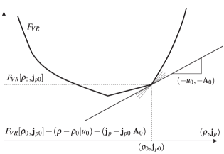
Figure 1: Schematic illustration of the subdifferential $\underline{\partial}{F}_{\text{VR}}[\rho_{0},\mathbf{j}_{\text{p}0}]$: The set of all slopes (potentials $-(u,\mathbf{A})$) of just-touching tangent planes entirely below the graph at $(\rho_{0},\mathbf{j}_{\text{p}0})$. One particular tangent, with slope $-(u_{0},\mathbf{A}_{0})$, is shown, while others are indicated by dashed lines. A similar illustration can be made of the superdifferential $\bar{\partial}\bar{E}[u,\mathbf{A}]$.

Analogously, we consider the concave energy functional $\bar{E}[u,\mathbf{A}]$ and its supergradients. In general, $(\rho_{0},\mathbf{j}_{\text{p}0})\in X_{\text{p}}$ is a supergradient of $\bar{E}$ at $(u_{0},\mathbf{A}_{0})\subset X_{\text{p}}^{\ast}$ if and only if $-(\rho_{0},\mathbf{j}_{\text{p}0})$ is a subgradient of the convex functional $-\bar{E}$ at $(u_{0},\mathbf{A}_{0})$. Hence, $(\rho_{0},\mathbf{j}_{\text{p}0})$ is a supergradient of $\bar{E}$ at $(u_{0},\mathbf{A}_{0})$ if the inequality

$$\bar{E}[u,\mathbf{A}]\leq\bar{E}[u_{0},\mathbf{A}_{0}]+(\rho_{0}|u-u_{0})+(\mathbf{j}_{\text{p}0}|\mathbf{A}-\mathbf{A}_{0})$$ (32)

holds for all $(u,\mathbf{A})\in X_{\text{p}}^{*}$. This condition is satisfied precisely when $(\rho_{0},\mathbf{j}_{\text{p}0})$ is the density arising from a (possibly degenerate) ground state of $\bar{H}[u_{0},\mathbf{A}_{0}]$. The superdifferential $\bar{\partial}\bar{E}[u_{0},\mathbf{A}_{0}]$ is the collection of all supergradients of $\bar{E}$ at $(u_{0},\mathbf{A}_{0})$.

For all ground-state densities $(\rho_{0},\mathbf{j}_{\text{p}0})$ and associated potentials $(u_{0},\mathbf{A}_{0})$, we now have the following stationary conditions of the HK and Lieb variation principles in Eqs. (26) and (29), respectively:

$$-(u_{0},\mathbf{A}_{0}) \in\underline{\partial}{F}_{\text{VR}}[\rho_{0},\mathbf{j}_{\text{p}0}],\quad (\rho_{0},\mathbf{j}_{\text{p}0}) \in\mathcal{B}_{N}^{\text{p}}\cap X,$$ (33)

$$(\rho_{0},\mathbf{j}_{\text{p}0}) \in\bar{\partial}\bar{E}[u_{0},\mathbf{A}_{0}],\quad (u_{0},\mathbf{A}_{0}) \in\mathcal{U}_{N}\cap X^{\ast}.$$ (34)

Importantly, these conditions are equivalent: $-(u_{0},\mathbf{A}_{0})$ is a subgradient of $F_{\text{VR}}$ at $(\rho_{0},\mathbf{j}_{\text{p}0})$ if and only if $(\rho_{0},\mathbf{j}_{\text{p}0})$ is a supergradient of $\bar{E}$ at $(u_{0},\mathbf{A}_{0})$. Hence, instead of a one-to-one mapping between individual potentials and individual ground-state densities, the convexity and concavity of the intrinsic and extrinsic energies, respectively, establish a mapping between the convex sets $\{(\rho,\mathbf{j}_{\text{p}})\}\subset X_{\text{p}}$ of degenerate ground-state densities and convex sets $\{(u,\mathbf{A})\}\subset X_{\text{p}}^{*}$ of potentials that give rise to identical ground-state densities; see Fig. 2.

The sub- and superdifferentials are empty when no minimizer and maximizer exist in the corresponding optimization problems in Eqs. (26) and (29). However, it is a general result of convex analysis that the subgradients (supergradients) of a convex (concave) function (under certain semicontinuity conditions) exist at a dense subset of the domain of the function. In CDFT, this result implies that the set of ground-state densities $(\rho_{0},\mathbf{j}_{\text{p},0})$ is dense in the set of all densities and that the set of potentials $(u_{0},\mathbf{A}_{0})$ that support a ground state is dense in the set of potentials.

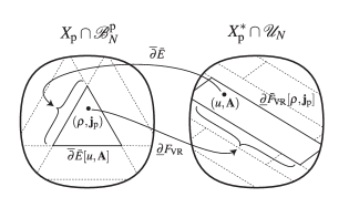
Figure 2: Illustration of considerations in Sec. III.6. Instead of a one-to-one mapping of individual potential pairs and corresponding ground-state density pairs, the sub- and superdifferentials of $F_{\text{VR}}$ and $\bar{E}$, respectively, maps (ground-state) densities into convex sets of (ground-state) potentials and potentials into convex sets of densities.

III.7 Degeneracies in CDFT

Consider now the case of degenerate ground-state densities in Eq. (26). For a finite degeneracy $G_{\text{d}}$, the superdifferential of the ground-state energy in the external potential $(u_{0},\mathbf{A}_{0})$ is then a $({G_{\text{d}}}-1)$-dimensional simplex with $G_{\text{d}}$ pure-state densities $(\rho_{0}^{i},\mathbf{j}_{\text{p}0}^{i})$ at the vertices:

$$\bar{\partial}{\bar{E}}[u_{0},\mathbf{A}_{0}]=\operatorname{co}\{(\rho_{0}^{i},\mathbf{j}_{\text{p},0}^{i}),\,|\,i=1,G_{\text{d}}\},$$ (35)

see Fig. 3 for an illustration. Consequently, each ground-state density $(\rho_{0},\mathbf{j}_{\text{p}0})$ may be written as convex combination of the $G_{\text{d}}$ pure-state densities,

$$(\rho_{0},\mathbf{j}_{\text{p}0})=\sum_{i=1}^{G_{\text{d}}}\lambda_{i}(\rho_{0}^{i},\mathbf{j}_{\text{p}0}^{i}),\;\sum_{i=1}^{G_{\text{d}}}\lambda_{i}=1,\;\lambda_{i}\geq 0.$$ (36)

As is well known, such degeneracies are either accidental or caused by symmetries of the Hamiltonian.

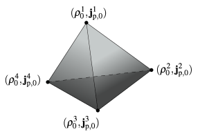
Figure 3: Illustration of the set $\bar{\partial}\bar{E}[u,\mathbf{A}]$ of ground state densities for potentials $(u,\mathbf{A})$ with degeneracy $G_{\text{d}}=4$. This is a convex set, a three-dimensional simplex, with vertices at $(\rho_{0}^{i},\mathbf{j}_{\text{p},0}^{i})$, i.e., $\bar{\partial}\bar{E}[u,\mathbf{A}]=\operatorname{co}\{(\rho_{0}^{i},\mathbf{j}_{\text{p},0}^{i})\}.$ In this example, we embed the simplex in $\mathbb{R}^{3}$, but in reality it is a three-dimensional subset of the density space $X_{\text{p}}$. The corresponding set of potentials is also a convex set, but usually with a more complicated structure. See also Fig. 2.

Consider next a ground-state density $(\rho_{0},\mathbf{j}_{\text{p}0})$ with several maximizing potentials in the Lieb variation principle in Eq. (29). Like the superdifferential of the ground-state energy, the subdifferential of the Vignale–Rasolt density functional is a convex set. Let now $(u_{0},\mathbf{A}_{0})$ be a potential with ground-state density $(\rho_{0},\mathbf{j}_{\text{p}0})$ and consider the family of external potentials

$$(u_{0}(\lambda),\mathbf{A}_{0}(\lambda))=(u_{0},\mathbf{A}_{0})+\lambda(\Delta u_{0},\Delta\mathbf{A}_{0}),$$ (37)

for some potential $(\Delta u_{0},\Delta\mathbf{A}_{0})$ and $\lambda\in\mathbb{R}$. The associated Hamiltonians are given by

$$\bar{H}[u_{0}(\lambda),\mathbf{A}_{0}(\lambda)] =\bar{H}[u_{0},\mathbf{A}_{0}]+\lambda K,$$ (38)

$$K =\sum\nolimits_{i}[\Delta u_{0}(\mathbf{r}_{i})+\frac{1}{2}\{\mathbf{p}_{i},\Delta\mathbf{A}_{0}(\mathbf{r}_{i})\}].$$ (39)

where $\{\Lambda,\Omega\}$ denotes the anti-commutator. Clearly, if $\bar{H}[u_{0},\mathbf{A}_{0}]$ and $K$ commute,

$$\left[\bar{H}[u_{0},\mathbf{A}_{0}],K\right]=0,$$ (40)

then $\bar{H}[u_{0}(\lambda),\mathbf{A}_{0}(\lambda)]$ has the same eigenstates for all $\lambda$. In particular, as $\lambda$ changes continuously from $0$, the external potentials in Eq. (37) will have the same ground-state density $(\rho_{0},\mathbf{j}_{\text{p}0})$ until a level crossing with the ground state occurs for $\bar{H}[u_{0}(\lambda),\mathbf{A}_{0}(\lambda)]$, see Capelle and Vignale Capelle and Vignale (2002). We note that the commutation condition in Eq. (40) is sufficient but not necessary for the existence of degenerate maximizing potentials.

There may be several, independent perturbing potentials that commute with the reference Hamiltonian $\bar{H}[u_{0},\mathbf{A}_{0}]$. Assuming a finite degeneracy $G_{\text{p}}$ of these potentials, we may write the subdifferential of the Vignale–Rasolt density functional as a $(G_{\text{p}}-1)$-dimensional simplex

$$\underline{\partial}{F}_{\text{VR}}[\rho_{0},\mathbf{j}_{\text{p}0}]=-\operatorname{co}\{(u_{0}^{i},\mathbf{A}_{0}^{i}),\,|\,i=1,G_{\text{p}}\}.$$ (41)

All potentials with the ground-state density $(\rho_{0},\mathbf{j}_{\text{p}0})$ may then be written as a convex combination,

$$(u_{0},\mathbf{A}_{0})=\sum_{i=1}^{G_{\text{p}}}\lambda_{i}(u_{0}^{i},\mathbf{A}_{\text{p}0}^{i}),\;\sum_{i=1}^{G_{\text{p}}}\lambda_{i}=1,\;\lambda_{i}\geq 0,$$ (42)

of the $G_{\text{p}}$ vertex potentials $(u_{0}^{i},\mathbf{A}_{0}^{i})$.

Consider now the special case of DFT, for which the HK and Lieb variation principles are given by Eqs. (8a) and (8b), where $E[v]$ and $F[\rho]$ depend only on the scalar potential and the electron density, respectively. Let $v_{0}$ be a potential with ground-state density $\rho_{0}$. Clearly, the only scalar potentials $v(\mathbf{r})$ that commute with the Hamiltonian $H[v_{0}]$ are the constant potentials $c$. It follows that the subdifferential of $F$ at $\rho_{0}$ is the convex set

$$\underline{\partial}{F}[\rho_{0}]=-\{v_{0}(\mathbf{r})+c\,|\,c\in\mathbb{R}\},$$ (43)

which may be regarded as a one-dimensional simplex with vertices $-v_{0}(\mathbf{r})\pm\infty$. In DFT, therefore, the ground-state density $\rho_{0}$ determines the external potential $v_{0}(\mathbf{r})$ uniquely up to an additive constant $c$, in accordance with the HK theorem.

Returning to CDFT, consider next two potentials $(u_{1},\mathbf{A}_{1})$ and $(u_{2},\mathbf{A}_{2})$ with the same ground-state density $(\rho_{0},\mathbf{j}_{\text{p}0})$. By the convexity of the subgradient of $F_{\text{VR}}$, all convex combinations

$$(u,\mathbf{A})=\lambda(u_{1},\mathbf{A}_{1})+(1-\lambda)(u_{2},\mathbf{A}_{2}),\quad 0\leq\lambda\leq 1$$ (44)

then have the same ground-state density. Recalling that $u_{1}=v_{1}+\tfrac{1}{2}A_{1}^{2}$, $u_{2}=v_{2}+\tfrac{1}{2}A_{2}^{2}$, and $u=v+\tfrac{1}{2}A^{2}$, the characterization of the non-uniqueness given in Eq. (44) can be expressed in terms of the ordinary scalar potential $v$. If $(v_{1},\mathbf{A}_{1})$ and $(v_{2},\mathbf{A}_{2})$ give rise to the same density, then so do all potentials of the form

$$\begin{pmatrix}v\\ \mathbf{A}\end{pmatrix}=\begin{pmatrix}\lambda v_{1}+(1-\lambda)v_{2}+\tfrac{1}{2}\lambda(1-\lambda)|\mathbf{A}_{1}-\mathbf{A}_{2}|^{2}\\ \lambda\mathbf{A}_{1}+(1-\lambda)\mathbf{A}_{2}\end{pmatrix}$$ (45)

with $0<\lambda<1$. However, this set is not a convex set and not a subdifferential, due to the use of the $(v,\mathbf{A})$ rather than $(u,\mathbf{A})$ variables.

An advantage of the formulation of stationary conditions in CDFT in terms of sub- and superdifferentials is that differentiability is not required. In general, a sufficient condition for differentiability of a function at a point is that the function is continuous at this point and has a single sub- or supergradient there; in the absence of continuity, differentiability is not guaranteed. The ground-state energy is differentiable at all potentials $(u,\mathbf{A})$ that have a nondegenerate ground-state density, whereas the Vignale–Rasolt functional is in principle nowhere differentiable since we may always add a constant term $c$ to the potential without affecting the ground-state densities. However, assuming that this is the only cause of nondifferentiability of the potentials, we may in the absence of other degeneracies write

$$\frac{\delta F_{\text{VR}}[\rho,\mathbf{j}_{p}]}{\delta\rho(\mathbf{r})}=-u(\mathbf{r})-c,\quad\frac{\delta F_{\text{VR}}[\rho,\mathbf{j}_{\text{p}}]}{\delta\mathbf{j}_{\text{p}}(\mathbf{r})}=-\mathbf{A}(\mathbf{r}),$$ (46)

and

$$\frac{\delta\bar{E}[u,\mathbf{A}]}{\delta u(\mathbf{r})}=\rho(\mathbf{r}),\quad\frac{\delta\bar{E}[u,\mathbf{A}]}{\delta\mathbf{A}(\mathbf{r})}=\mathbf{j}_{\text{p}}(\mathbf{r}),$$ (47)

where $(\rho,\mathbf{j}_{\text{p}})$ is the (non-degenerate) ground-state density of the potential $(u,\mathbf{A})$.

III.8 Numerical calculation of $F_{\text{VR}}[\rho,\mathbf{j}_{\text{p}}]$

Besides allowing formal application of theorems in convex analysis to CDFT, the convex formulation given above has practical value. After linear programming and optimization of quadratic functions, optimization of convex and concave functions is the mathematically most well-characterized type of optimization problem. The fact that convex and concave optimization problems have a unique global optimum (either in the form a single point or a convex set of optimal points) and no additional local optima is of great value when devising practical optimization methods.

In standard DFT, Lieb’s formulation Lieb (1983) of $F[\rho]$ in terms of the Legendre–Fenchel transform of the concave energy functional $E[v]$ has proven useful in the study of functionals of interest in Kohn–Sham theory Colonna and Savin (1999); Wu and Yang (2003); Teale et al. (2009, 2010a, 2010b); Strømsheim et al. (2011). In particular, the modulation of the two-electron interaction operator $W$ by a parameter $\lambda$ such that,

$$W_{\lambda}=\sum_{i<j}w_{\lambda}(r_{ij}),\;w_{0}(r_{ij})=0,\;w_{1}(r_{ij})=1/r_{ij},$$ (48)

allows us to represent the ground-state energy $E_{\lambda}[v]$ at interaction strength $\lambda$ in terms of its conjugate functional $F_{\lambda}[\rho]$. The standard choice is $w_{\lambda}(r_{ij})=\lambda/r_{ij}$, but other choices are possible. If the density supplied to $F_{\lambda}[\rho]$ is held fixed at a physical density generated by an appropriate (high-level, systematically improvable) ab-initio quantum-chemical methodology and if the value of the interaction-strength parameter is varied from $0$ to $1$, then the adiabatic connection Harris and Jones (1974); Langreth and Perdew (1975); Gunnarsson and Lundqvist (1976, 1977); Langreth and Perdew (1977) between the Kohn–Sham ($\lambda=0$) and physical ($\lambda=1$) systems can be studied numerically. Such studies for atomic and molecular species Colonna and Savin (1999); Teale et al. (2009, 2010a, 2010b); Strømsheim et al. (2011) can provide useful insight into the failings of standard density-functional approximations and provide data for the construction and evaluation of new forms, based on the modeling of the adiabatic connection Becke (1998); Seidl et al. (1999, 2000); Gori-Giorgi et al. (2009); Cohen et al. (2007); Teale et al. (2010a).

Having established a convex formulation of CDFT in Sec. III.5, it is possible to calculate the adiabatic connection in CDFT in a manner similar to that of standard DFT. Details of the adiabatic connection for CDFT have been presented previously by Liu Liu (1996). The ground-state energy functionals at interaction strength $\lambda$ are given by

$$E_{\lambda}[v,\mathbf{A}] =\inf_{\Gamma}\mathrm{Tr}({\Gamma H_{\lambda}[v,\mathbf{A}]}),$$ (49)

$$\bar{E}_{\lambda}[u,\mathbf{A}] =E_{\lambda}[u-\tfrac{1}{2}A^{2},\mathbf{A}],$$ (50)

where we have introduced the Hamiltonian

$$H_{\lambda}[v,\mathbf{A}]=\frac{1}{2}\sum_{k}\pi_{k}^{2}+\sum_{k}v(\mathbf{r}_{k})+W_{\lambda}.$$ (51)

From the exact functional $\bar{E}_{\lambda}[u,\mathbf{A}]$ or an accurate approximation to it, the adiabatic connection may be studied in terms the corresponding Vignale–Rasolt functional

$$F_{\mathrm{VR},\lambda}[\rho,\mathbf{j}_{\text{p}}]=\sup_{u,\mathbf{A}}\left[\bar{E}_{\lambda}[u,\mathbf{A}]-(\rho|u)-(\mathbf{j}_{\text{p}}|\mathbf{A})\right],$$ (52)

which needs to be evaluated for a fixed density $(\rho,\mathbf{j}_{\text{p}})$ and different values of $\lambda$ in the interval $0\leq\lambda\leq 1$. Typically, the density is the ground-state density for some external potential $(v_{\text{ext}},\mathbf{A}_{\text{ext}})$ at $\lambda=1$. The optimization in Eq. (52) is trivial for $\lambda=1$ since the optimal potential is then $(v_{\mathrm{ext}}+\tfrac{1}{2}A_{\text{ext}}^{2},\mathbf{A}_{\mathrm{ext}})$; for $0\leq\lambda<1$, the optimization is non-trivial. In particular, for $\lambda=0$, the optimal potential is the Kohn–Sham potential $(u_{\text{s}},\mathbf{A}_{\text{s}})$ given by

$$u_{\text{s}} =v_{\text{ext}}+v_{\text{J}}+v_{\mathrm{xc}}+\tfrac{1}{2}A_{\text{s}}^{2}=v_{\text{s}}+\tfrac{1}{2}A_{\text{s}}^{2},$$ (53)

$$\mathbf{A}_{\text{s}} =\mathbf{A}_{\text{ext}}+\mathbf{A}_{\text{xc}},$$ (54)

where the classical Coulomb or Hartree potential $v_{\text{J}}$ and the exchange–correlation potential $v_{\text{xc}}$ are the functional derivatives of the corresponding energy components as in standard Kohn–Sham DFT. The exchange–correlation contribution to the vector potential is defined as

$$\mathbf{A}_{\mathrm{xc}}=\frac{\delta E_{\mathrm{xc}}[\rho,\mathbf{j}_{\text{p}}]}{\delta\mathbf{j}_{\text{p}}},$$ (55)

where differentiability in relevant directions is assumed. These scalar and vector potentials then enter the CDFT Kohn–Sham equations Vignale and Rasolt (1987), which may be re-written in terms of $(u_{\text{s}},\mathbf{A}_{\text{s}})$ as

$$\left[\tfrac{1}{2}p^{2}+\tfrac{1}{2}\{\mathbf{p},\mathbf{A}_{\text{s}}\}+u_{\text{s}}\right]\varphi_{p}=\varepsilon_{p}\varphi_{p}.$$ (56)

If the spin dependent $\mathbf{B}(\mathbf{r}_{k})\cdot\mathbf{S}$ term is included in the Hamiltonian of Eq. (10) with the modified interactions of Eq. (48), then similar arguments apply. Two-component spinors rather than one-particle orbitals then occur in the Kohn–Sham equations, allowing for a treatment of non-collinear magnetism.

Even in the absence of external magnetic fields, violations of non-interacting $v$-representability—that is, the existence of a ground-state density of the fully interacting Hamiltonian $H_{1}[v,\mathbf{A}]$ that cannot be reproduced by Slater-determinantal ground-states of the non-interacting Hamiltonian $H_{0}[v_{\text{s}},\mathbf{A}_{\text{s}}]$—have been shown to be common in two-electron systems Taut et al. (2009). In general, an extended Kohn–Sham formalism, allowing for an ensemble description and fractional occupation numbers, is therefore required in CDFT as well as in standard DFT.

To facilitate the optimization of $F_{\mathrm{VR},\lambda}[\rho,\mathbf{j}_{\text{p}}]$ at a general interaction strength $\lambda$, we restrict our attention to classes of potentials that can be parameterized in a simple way—for example, as linear combinations of basis functions. The most direct way to benefit from the concavity of $\bar{E}[u,\mathbf{A}]$ is to parameterize $u$ rather than $v$ in the affine form

$$u(\mathbf{r}) =u_{\text{ref}}(\mathbf{r})+\sum_{t}b_{t}f_{t}(\mathbf{r}),$$ (57)

$$\mathbf{A}(\mathbf{r}) =\mathbf{A}_{\text{ref}}(\mathbf{r})+\sum_{t}\mathbf{c}_{t}g_{t}(\mathbf{r}).$$ (58)

The use of $u$ rather than $v$ eliminates the $A^{2}$ term and the associated quadratic dependence on $\mathbf{c}_{t}$, thereby simplifying the equations obtained upon substitution in Eq. (52). Importantly, it also ensures that all stationary points are true global maxima. To perform optimizations similar to those in Refs. Wu and Yang (2003); Teale et al. (2009, 2010a, 2010b); Strømsheim et al. (2011), all that remains is to be able to calculate the ground-state energy $\bar{E}_{\lambda}[u,\mathbf{A}]$ with sufficient accuracy and to choose appropriate basis functions $\{f_{t}\}$ and $\{g_{t}\}$. Derivatives with respect to the expansion coefficients $b_{t}$ and $\mathbf{c}_{t}$ may then be used in a quasi-Newton procedure analogous to that in Ref. Wu and Yang (2003). The choice of basis functions and reference potentials raises the issue of a balanced descriptions of $u$ and $\mathbf{A}$, as well as the asymptotic limits and reduction of gauge freedom inherent in the finite basis set. Although important for practical implementation, these issues are beyond the scope of this article.

III.9 A note on spin densities

The formulation of CDFT with $(u,\mathbf{A})$ as the basic potential and with the intrinsic and extrinsic energies expressed as mutual Legendre–Fenchel transforms makes the introduction of spin straightforward. The addition of the spin-Zeeman operator to the Hamiltonian introduces an energy term containing the spin density $\mathbf{m}(\mathbf{r})$ paired with the magnetic field, $(\mathbf{m}|\mathbf{B})=(\mathbf{m}|\nabla\times\mathbf{A})$. A partial integration transfers the curl operator to the spin density and gives a surface term if the integration domain is finite. Neglect of the surface term leads to the energy term

$$(\mathbf{m}|\nabla\times\mathbf{A})=(\boldsymbol{\nabla}\times\mathbf{m}|\mathbf{A})$$ (59)

and a theory with $(\rho,\mathbf{j}_{\text{m}})$ as the basic density. Here,

$$\mathbf{j}_{\text{m}}=\mathbf{j}_{\text{p}}+\nabla\times\mathbf{m},$$ (60)

is the sum of the paramagnetic current and the spin current $\nabla\times\mathbf{m}$. All results above remain valid with $\mathbf{j}_{\text{p}}$ replaced by $\mathbf{j}_{\text{m}}$ and with suitable modifications of the Hamiltonian and definitions of $\mathcal{V}_{N}$ and $\mathcal{B}_{N}^{\text{p}}$.

The use of $\mathbf{j}_{\text{m}}$ as a basic density has been discussed by Capelle and Gross Capelle and Gross (1997) as a way to translate functionals between spin-density functional theory (SDFT) and CDFT. The alternative formulation of current-spin DFT (CSDFT) in terms of the charge density $\rho$, the spin density $\mathbf{m}$, and the paramagnetic current density $\mathbf{j}_{\text{p}}$ as separate basic variables is a less attractive formal theory since two independent potentials such as $(u,\mathbf{A})$ cannot be conjugate to three independent densities $(\rho,\mathbf{m},\mathbf{j}_{\text{p}})$. On the other hand, construction of practical approximate exchange–correlation functionals may be substantially more difficult with the basic variables $\rho$ and $\mathbf{j}_{\text{m}}$.

IV The physical current as a basic variable

Mathematically, it is not surprising that a theory formulated in terms of magnetic vector potentials and wave functions—both gauge-dependent objects—makes use of gauge-dependent basic variables. Indeed, with gauge-dependent notions being so deeply entrenched in the theory, it is not trivial to construct a useful reformulation that features only gauge-invariant basic variables. On the other hand, from a physical point of view, it is somewhat unappealing that the paramagnetic current, rather than the physical current, arises as a basic density. Therefore, some authors have attempted the construction of an alternative CDFT, with the physical current as a basic variable. In particular, Pan and Sahni have gone far in arguing that the paramagnetic current density, in some sense, cannot correctly be regarded as a basic CDFT variable Pan and Sahni (2010, 2012a); Sahni and Pan (2012); Pan and Sahni (2012b).

IV.1 Do physical densities determine potentials up to a gauge?

An important question that arises in CDFT is to what extent an HK theorem is possible when the physical densities $(\rho,\mathbf{j})$ are chosen as the basic densities—that is, whether $(v_{1},\mathbf{A}_{1})\nsim(v_{2},\mathbf{A}_{2})$ always implies that $(\rho_{1},\mathbf{j}_{1})\neq(\rho_{2},\mathbf{j}_{2})$.

Two simple observations lend plausibility to this claim. First, for one-electron systems, $(v,\mathbf{A})$ can be found explicitly given $(\rho,\mathbf{j})$. Writing the one-electron wave function as

$$\psi(\mathbf{r})=R(\mathbf{r})\text{e}^{\text{i}S(\mathbf{r})},$$ (61)

where $R$ and $S$ are real valued, we obtain the density $\rho=R^{2}$ and physical current density $\mathbf{j}=\rho(\boldsymbol{\nabla}S+\mathbf{A})$. Because of the identity $\boldsymbol{\nabla}\times\boldsymbol{\nabla}S=\mathbf{0}$, the physical densities $\rho$ and $\mathbf{j}$ determine the external magnetic field,

$$\mathbf{B}(\mathbf{r})=\boldsymbol{\nabla}\times\mathbf{A}(\mathbf{r})=\boldsymbol{\nabla}\times\frac{\mathbf{j(\mathbf{r})}}{\rho(\mathbf{r})}.$$ (62)

The scalar potential $v$ may be determined up to a constant from the eigenvalue equation $(\tfrac{1}{2}\pi^{2}+v-E)\psi=0$ and the observation that $\boldsymbol{\pi}=-\text{i}\boldsymbol{\nabla}+\mathbf{A}=-\text{i}\boldsymbol{\nabla}+\mathbf{j}/\rho-\boldsymbol{\nabla}S$, yielding

$$\left[\frac{1}{2}\left(-\mathrm{i}\boldsymbol{\nabla}+\frac{\mathbf{j}(\mathbf{r})}{\rho(\mathbf{r})}\right)^{2}+v(\mathbf{r})-E\right]\rho^{1/2}(\mathbf{r})=0,$$ (63)

from which $v(\mathbf{r})-E$ is uniquely determined. Hence, for a one-electron system, $\mathbf{B}$ and $v$ are both determined by $\rho$ and $\mathbf{j}$. For an $N$-electron system, we obtain more generally

$$\boldsymbol{\nabla}\times\frac{\mathbf{j(\mathbf{r})}}{\rho(\mathbf{r})}=\boldsymbol{\nu}(\mathbf{r})+\mathbf{B}(\mathbf{r}),$$ (64)

where $\boldsymbol{\nu}=\boldsymbol{\nabla}\times\rho^{-1}\mathbf{j}_{\text{p}}$ is the vorticity introduced by Vignale and Rasolt Vignale and Rasolt (1987). Vorticity is a gauge-invariant quantity, but it is not clear whether it can be uniquely reconstructed from $(\rho,\mathbf{j})$, without a priori knowledge of the external magnetic field $\mathbf{B}$.

Following Pan and Sahni Pan and Sahni (2010), the second observation is that, while there is no HK theorem for CDFT in terms of paramagnetic densities, the counterexamples to the existence of an HK theorem for paramagnetic densities (such as the harmonic-oscillator system in Sec. III.3) do not preclude an HK theorem for physical densities.

To see this, note that these counterexamples all exhibit different potentials $(v_{1},\mathbf{A}_{1})\nsim(v_{2},\mathbf{A}_{2})$ with the same ground state $\psi_{1}=\psi_{2}$ and therefore the same paramagnetic density $(\rho_{1},\mathbf{j}_{\text{p}1})=(\rho_{2},\mathbf{j}_{\text{p}2})$. However, according to the original HK theorem, this situation is impossible when $\mathbf{A}_{1}=\mathbf{A}_{2}$ since this would imply $v_{2}\neq v_{1}+c$ and therefore $\rho_{1}\neq\rho_{2}$. We must therefore assume that $\mathbf{A}_{1}\neq\mathbf{A}_{2}$ in the counterexamples. However, from the assumption $\mathbf{j}_{\text{p}1}=\mathbf{j}_{\text{p}2}$, it then follows that $\mathbf{j}_{1}-\mathbf{j}_{2}=\rho_{1}(\mathbf{A}_{1}-\mathbf{A}_{2})\neq\mathbf{0}$. In short, if $(v_{1},\mathbf{A}_{1})\nsim(v_{2},\mathbf{A}_{2})$ share the same ground-state wave function, then the physical densities are not the same. It remains to explore whether it is possible to have different ground states $\psi_{1}\neq\psi_{2}$ but the same physical densities $(\rho_{1},\mathbf{j}_{1})=(\rho_{2},\mathbf{j}_{2})$; if possible, then no HK theorem exists for the physical current densities.

General arguments for an HK theorem for physical current densities have been put forth by Pan and Sahni Pan and Sahni (2010, 2012a) and by Diener Diener (1991). However, as discussed below, neither of these arguments amounts to a rigorous proof. To our knowledge, the existence of an HK theorem for physical current densities therefore remains open.

IV.2 Pan and Sahni’s argument

The standard HK theorem of DFT states that $v\neq v^{\prime}+c$ implies $\rho^{\prime}\neq\rho^{\prime}$. The proof has two parts: first, it is shown that scalar potentials that differ by more than a constant must have different wave functions $\psi$ and $\psi^{\prime}$; second, this result is combined with the Rayleigh–Ritz variation principle to show that the assumptions $\rho=\rho^{\prime}$ and $v\neq v^{\prime}+c$ lead to a contradiction. It follows that $v\neq v^{\prime}+c$ implies $\rho\neq\rho^{\prime}$.

For CDFT with physical densities, a proof along the same lines has been attempted by Pan and Sahni Pan and Sahni (2010). The first part of their argument establishes that different potentials $(v,\mathbf{A})\nsim(v^{\prime},\mathbf{A}^{\prime})$ cannot yield the same physical density $(\rho_{0},\mathbf{j}_{0})=(\rho^{\prime}_{0},\mathbf{j}^{\prime}_{0})$ if the ground-state wave functions are the same. That is, without loss of generality, it may be assumed in an HK-type argument that the wave functions are different. The second part of their argument seeks to establish, by the Rayleigh–Ritz variation principle, that gauge-inequivalent potentials cannot have both different ground-state wave functions and the same physical ground-state density. To this end, two potentials $(v,\mathbf{A}),(v^{\prime},\mathbf{A}^{\prime})\in\mathcal{V}_{N}$, $(v,\mathbf{A})\neq(v^{\prime},\mathbf{A}^{\prime})$, are considered and it is argued that a contradiction arises from the following assumptions:

• The potentials have the same physical density $(\rho_{0},\mathbf{j}_{0})$.

• The potentials differ by more than a gauge transformation, $(v^{\prime},\mathbf{A}^{\prime})\nsim\ (v,\mathbf{A})$.

No contradiction can result from (a) alone, so the assumption (b) is crucial for any reductio ad absurdum argument to succeed. For example, because of gauge freedom, (a) and the negation of (b) are certainly not contradictory since this corresponds to the perfectly consistent situation where two potentials that differ by a gauge transformation give rise to the same physical density. A correct proof must therefore contain at least one step that makes use of (b). However, while stated as an assumption, (b) is in fact never used in Pan and Sahni’s argument. The argument must consequently be invalid.

In more detail, we here identify an erroneous step in the reasoning in Ref. Pan and Sahni (2010), in particular Eqs. (35)–(40). With $\psi$ and $\psi^{\prime}$ denoting the ground states of the two potentials, we obtain Eq. (35) from Ref. Pan and Sahni (2010):

$$E=\langle{\psi}|H[v,\mathbf{A}]|{\psi}\rangle<\langle{\psi^{\prime}}|H[v,\mathbf{A}]|{\psi^{\prime}}\rangle.$$ (65)

The identity $H[v,\mathbf{A}]=H[v^{\prime},\mathbf{A}^{\prime}]+(H[v,\mathbf{A}]-H[v^{\prime},\mathbf{A}^{\prime}])$ yields for the expectation value on the right-hand side

$$\begin{split}\langle{\psi^{\prime}}|H[v,\mathbf{A}]|{\psi^{\prime}}\rangle&=E^{\prime}+\langle{\psi^{\prime}}|\tfrac{1}{2}\pi^{2}+v-\tfrac{1}{2}\pi^{\prime 2}-v^{\prime}|{\psi^{\prime}}\rangle\\ &=E^{\prime}+\langle{\psi^{\prime}}|\tfrac{1}{2}\{\boldsymbol{\pi},\mathbf{A}\}+v-\tfrac{1}{2}A^{2}-\tfrac{1}{2}\{\boldsymbol{\pi}^{\prime},\mathbf{A}^{\prime}\}-v^{\prime}+\tfrac{1}{2}A^{\prime 2}|{\psi^{\prime}}\rangle.\end{split}$$ (66)

It is here important to distinguish between $\boldsymbol{\pi}=\mathbf{p}+\mathbf{A}$ and $\boldsymbol{\pi}^{\prime}=\mathbf{p}+\mathbf{A}^{\prime}$ since the representation of the mechanical momentum operator is gauge and vector-potential dependent. To proceed, we explicitly write out the corresponding physical current density operators, which for the two potentials are given by

$$\hat{\mathbf{j}}(\mathbf{r}) =\frac{1}{2}\sum_{k}(\boldsymbol{\pi}_{k}\delta(\mathbf{r}_{k}-\mathbf{r})+\delta(\mathbf{r}_{k}-\mathbf{r})\boldsymbol{\pi}_{k}),$$ (67)

$$\hat{\mathbf{j}}^{\prime}(\mathbf{r}) =\frac{1}{2}\sum_{k}(\boldsymbol{\pi}^{\prime}_{k}\delta(\mathbf{r}_{k}-\mathbf{r})+\delta(\mathbf{r}_{k}-\mathbf{r})\boldsymbol{\pi}^{\prime}_{k}).$$ (68)

From these, we may calculate the physical current (assumed to be the same in the two cases) and its interaction with some vector potential $\mathbf{a}(\mathbf{r})$ as

$$\mathbf{j}_{0}(\mathbf{r}) =\langle{\psi}|\hat{\mathbf{j}}(\mathbf{r})|{\psi}\rangle=\langle{\psi^{\prime}}|\hat{\mathbf{j}}^{\prime}(\mathbf{r})|{\psi^{\prime}}\rangle$$ (69)

$$(\mathbf{j}_{0}|\mathbf{a}) =\langle{\psi}|\tfrac{1}{2}\{\boldsymbol{\pi},\mathbf{a}\}|{\psi}\rangle=\langle{\psi^{\prime}}|\tfrac{1}{2}\{\boldsymbol{\pi}^{\prime},\mathbf{a}\}|{\psi^{\prime}}\rangle,$$ (70)

where it is important to use primed or unprimed quantities consistently. To ensure that we are using the correct current-density operator for $\psi^{\prime}$ in Eq. (66), we insert the identity $\{\boldsymbol{\pi},\mathbf{A}\}=\{\boldsymbol{\pi}^{\prime}+\mathbf{A}-\mathbf{A}^{\prime},\mathbf{A}\}$ yielding,

$$\begin{split}E<E^{\prime}+(\rho_{0}|\Delta v)+(\mathbf{j}_{0}|\Delta\mathbf{A})+\tfrac{1}{2}(\rho_{0}|\Delta A^{2}).\end{split}$$ (71)

where we have introduced $\Delta v=v-v^{\prime}$ and $\Delta\mathbf{A}=A-A^{\prime}$ and also used the inequality in Eq. (65).

Carrying out the above argument with primed and unprimed variables interchanged, we obtain the strict inequality

$$E+E^{\prime}<E^{\prime}+E+(\rho_{0}|\Delta A^{2}),$$ (72)

where the last term does not vanish since $\Delta A^{2}$ is symmetric in the primed and unprimed variables. In agreement with the HK theorem, a contradiction arises if (and only if) $\mathbf{A}=\mathbf{A}^{\prime}$. When $\mathbf{A}(\mathbf{r})$ and $\mathbf{A}^{\prime}(\mathbf{r})$ differ where $\rho(\mathbf{r})\neq 0$ (as a result of different physical fields or by a gauge transformation), no contradiction arises.

In the argument given in Ref. Pan and Sahni (2010), the authors incorrectly identify $\langle{\psi^{\prime}}|\hat{\mathbf{j}}(\mathbf{r})|{\psi^{\prime}}\rangle$ and $\langle{\psi^{\prime}}|\hat{\mathbf{j}}^{\prime}(\mathbf{r})|{\psi^{\prime}}\rangle$, leading to their Eq. (38), which differs from Eq. (71) above by the replacement of $\tfrac{1}{2}(\rho_{0}|\Delta A^{2})$ with $\tfrac{1}{2}(\rho_{0}|A^{\prime 2}-A^{2})$. Since their term is antisymmetric rather than symmetric in the primed and unprimed variables, the authors obtain a contradiction $E+E^{\prime}<E+E^{\prime}$ irrespective of $\mathbf{A}$ and $\mathbf{A}^{\prime}$, leading to the unjustified conclusion that ($\rho_{0},\mathbf{j}_{0})$ determines $(v,\mathbf{A})$.

IV.3 Diener’s argument

An earlier attempt to prove an HK-type theorem for physical currents by Diener Diener (1991) invokes an intriguing strategy for eliminating the term $(\rho_{0}|\Delta A^{2})$ from Eq. (72). The key idea is to replace the external vector potential $\mathbf{A}$ by an effective vector potential $\mathbf{a}_{\text{eff}}[\mathbf{j},\psi]$ defined to reproduce a given physical current density $\mathbf{j}$ from a given wave function $\psi$ so that

$$\mathbf{j}=\mathbf{j}_{\text{p};\psi}+\rho_{\psi}\mathbf{a}_{\text{eff}}[\mathbf{j},\psi].$$ (73)

Consider now the following rearrangement of the kinetic energy term

$$\pi^{2} =p^{2}+\{\mathbf{p},\mathbf{A}\}+A^{2}$$

$$=p^{2}-a_{\text{eff}}^{2}+\{\mathbf{p}+\mathbf{a}_{\text{eff}},\mathbf{A}\}+(\mathbf{a}_{\text{eff}}-\mathbf{A})^{2}.$$ (74)

By definition, $\frac{1}{2}\langle{\psi}|\{\mathbf{p}+\mathbf{a}_{\text{eff}}[\mathbf{j},\psi],\mathbf{A}\}|{\psi}\rangle=(\mathbf{j}|\mathbf{A})$. For a prescribed physical current density $\mathbf{j}_{0}$, the expectation value of an arbitrary wave function is then

$$\langle{\psi}|H[v,\mathbf{A}]|{\psi}\rangle =\langle{\psi}|\tfrac{1}{2}(p^{2}-a_{\text{eff}}^{2})+W|{\psi}\rangle$$

$$+(\mathbf{j}_{0}|\mathbf{A})+(\rho|v)+\tfrac{1}{2}(\rho|(\mathbf{a}_{\text{eff}}-\mathbf{A})^{2}).$$ (75)

The total current evaluated using the effective momentum operator $\mathbf{p}+\mathbf{a}_{\text{eff}}$ instead of the true mechanical momentum operator $\mathbf{p}+\mathbf{A}$ always evaluates to the prescribed current $\mathbf{j}_{0}$. Diener then defines a universal density functional of the form

$$F_{\text{D}}[\rho,\mathbf{j}] =\inf_{\psi\mapsto\rho}\langle{\psi}|H_{\text{eff}}[\mathbf{j},\psi]|{\psi}\rangle,$$ (76)

$$H_{\text{eff}}[\mathbf{j},\psi] =\tfrac{1}{2}p^{2}-\tfrac{1}{2}a_{\text{eff}}[\mathbf{j},\psi]^{2}+W.$$ (77)

By exploiting this functional, Diener derives the inequality

$$\langle{\psi_{0}}|H[v,\mathbf{A}]|{\psi_{0}}\rangle\leq\langle{\psi^{\prime}_{0}}|H[v,\mathbf{A}]|{\psi^{\prime}_{0}}\rangle-\frac{1}{2}(\rho_{0}|\Delta A^{2}),$$ (78)

in lieu of the usual strict Rayleigh–Ritz inequality underlying the HK proof as given in Eq. (65). When $\psi^{\prime}_{0}$ is the ground state of potentials that differ by more than a gauge, $(v^{\prime},\mathbf{A}^{\prime})\nsim(v,\mathbf{A})$, the above non-strict inequality is (without further ado) taken to be strict in Diener’s presentation. If a strict inequality is accepted, a standard reductio ad absurdum proof is possible because the last term of Eq. (72) cancels to yield the contradiction $E+E^{\prime}<E^{\prime}+E$.

We now consider two technical problems not addressed by Diener. The first is that the expectation value being minimized in $F_{\text{D}}$ is not bounded from below for densities that vanish at some point. Although unusual, such ground-state densities can arise for small molecules in strong magnetic fields. Consider a wave function $\Phi_{0}$ giving rise to a density $\rho_{0}$ that vanishes at some point in space $\mathbf{O}$. Let us also introduce spherical coordinates $(r,\theta,\phi)$ about $\mathbf{O}$. Then, for the wave functions

$$\Phi_{m}(\mathbf{x}_{1},\ldots,\mathbf{x}_{N})=\text{e}^{2\pi\text{i}m\sum_{k=1}^{N}\phi_{k}}\Phi_{0}(\mathbf{x}_{1},\ldots,\mathbf{x}_{N})$$ (79)

with integer $m$, we see that $\Phi_{m}$ and $\Phi_{0}$ give rise to the same density $\rho_{0}$ but to different paramagnetic current densities related by

$$\mathbf{j}_{\text{p};m}=\frac{m\hat{\boldsymbol{\phi}}}{r\sin(\theta)}\rho_{0}+\mathbf{j}_{\text{p};0},$$ (80)

where $\hat{\boldsymbol{\phi}}$ is the unit vector in the direction specified by $\phi$. As a result,

$$\mathbf{a}_{m}=\mathbf{a}_{\text{eff}}[\mathbf{j},\Phi_{m}]=\mathbf{a}_{\text{eff}}[\mathbf{j},\Phi_{0}]-\frac{m\hat{\boldsymbol{\phi}}}{r\sin(\theta)}=\mathbf{a}_{0}-\frac{m\hat{\boldsymbol{\phi}}}{r\sin(\theta)}.$$ (81)

Calculating the expectation value of the effective Hamiltonian in Eq. (77), some terms arising from $\tfrac{1}{2}p^{2}$ cancel terms arising from $\tfrac{1}{2}a_{m}^{2}$, leaving

$$\langle{\Phi_{m}}|\tfrac{1}{2}(p^{2}-a_{m}^{2})+W|{\Phi_{m}}\rangle =\langle{\Phi_{0}}|\tfrac{1}{2}(p^{2}-a_{0}^{2})+W|{\Phi_{0}}\rangle$$

$$\ \ +m\int\frac{\hat{\boldsymbol{\phi}}\cdot\mathbf{j}}{r\sin(\theta)}\,\mathrm{d}\mathbf{r}.$$ (82)

For physical currents $\mathbf{j}$ with a nonzero last integral, for example a circular current, the expectation value can be decreased without bound, demonstrating that $F_{\text{D}}[\rho,\mathbf{j}]$ is not well defined on the full domain $\mathcal{B}_{N}$.

The second technical problem in the derivation of the inequality in Eq. (78) concerns the strategy of choosing a prescribed $\mathbf{j}_{0}$ such that the effective vector potential equals the external vector potential. This amounts to a self-consistency condition [Eq. (11) of Ref. Diener, 1991],

$$\mathbf{j}_{0}=\mathbf{j}_{\text{p};\Phi_{\text{D}}}+\rho_{0}\mathbf{a}_{\text{eff}}[\mathbf{j}_{0},\Phi_{\text{D}}]=\mathbf{j}_{\text{p};\Psi[v,\mathbf{A}]}+\rho_{0}\mathbf{A},$$ (83)

where $\Phi_{\text{D}}$ minimizes $\langle{\Phi_{\text{D}}}|H_{\text{eff}}[\mathbf{j}_{0},\Phi_{\text{D}}]|{\Phi_{\text{D}}}\rangle$ and $\Psi[v,\mathbf{A}]$ is the ground state of the external potentials giving rise to $(\rho_{0},\mathbf{j}_{0})$. Diener’s derivation of the inequality in Eq. (78) hinges on the ability to reproduce the paramagnetic current density from a ground state $\Psi[v,\mathbf{A}]$ of $H[v,\mathbf{A}]$ by a minimizing wave function in $F_{\text{D}}[\rho_{0},\mathbf{j}_{0}]$. However, it is unclear whether this is always possible.

IV.4 Constrained search with physical currents

In lieu of a rigorous proof for an HK-type theorem for physical currents, it is possible to proceed by conjecturing such a result and exploring its consequences. Additionally, an important point is that a mapping from ground state densities to potentials may not be required for a formulation of CDFT, provided that the theory can be constructed by some other means such as a constrained search or Legendre–Fenchel transformation formalism. We shall here explore such issues in the framework introduced by Pan and Sahni Pan and Sahni (2010, 2012a); Sahni and Pan (2012); Pan and Sahni (2012b) in more detail.

A complication due to the choice of the physical current as a basic variable is that constraints of the type “$\psi\to\rho,\mathbf{j}$” require explicit reference to a vector potential, because the physical current is not determined by the wave function alone. Care must therefore be exercised when developing a constrained-search formalism for physical currents.

For each magnetic field under consideration, we fix a gauge. Hence, we choose a mapping

$$\mathbf{B}(\mathbf{r})\mapsto\mathbf{a}[\mathbf{B}](\mathbf{r})$$ (84)

from magnetic fields to magnetic vector potentials, and also fix the constant shift of scalar potentials in some way. From the conjecture that a ground state density $(\rho,\mathbf{j})$ uniquely determines a gauge class of potentials $\overline{(v,\mathbf{A})}$, we may now write mappings

$$(\rho,\mathbf{j})\leftrightarrow(\nabla v,\mathbf{B})\leftrightarrow(v,\mathbf{a}[\mathbf{B}])$$ (85)

Hence, we may write the scalar potential, the external magnetic field and its vector potential as functionals $v=w[\rho,\mathbf{j}]$, $\mathbf{B}=\mathbf{b}[\rho,\mathbf{j}]$, and $\mathbf{A}=\mathbf{a}[\mathbf{b}[\rho,\mathbf{j}]]$ of the physical densities; these are representatives of the equivalence class $\overline{(v,\mathbf{A})}$.

Given potentials $(v,\mathbf{A})$, we may determine the corresponding ground state $\psi_{0}$ and physical ground-state densities $(\rho,\mathbf{j})\in\mathcal{B}_{N}$, and express the energy as

$$\begin{split}E[v,\mathbf{A}]=\langle{\psi_{0}}|\tfrac{1}{2}p^{2}+W|{\psi_{0}}\rangle+(\rho|v-\tfrac{1}{2}A^{2})+(\mathbf{j}|\mathbf{A}).\end{split}$$ (86)

Using the mapping from densities to potentials, a universal density functional could in principle internally reconstruct the ground state potentials, and obtain the intrinsic energy via

$$\begin{split}F_{\text{PS}}[\rho,\mathbf{j}]&=E\left[w[\rho,\mathbf{j}],\mathbf{a}[\mathbf{b}[\rho,\mathbf{j}]]\right]-(\rho\,|\,w[\rho,\mathbf{j}]-\tfrac{1}{2}a[\mathbf{b}[\rho,\mathbf{j}]]^{2})\\ &\ \ -(\mathbf{j}\,|\,\mathbf{a}[\mathbf{b}[\rho,\mathbf{j}]]).\end{split}$$ (87)

Furthermore, we may define a non-universal constrained-search functional that depends explicitly on the external vector potential,

$$\begin{split}F^{\text{cs1}}_{\text{PS}}[\rho,\mathbf{j},\mathbf{A}]&=\inf_{\Gamma\mapsto(\rho,\mathbf{j}-\rho\mathbf{A})}\mathrm{Tr}({\Gamma(\tfrac{1}{2}p^{2}+W)})\\ &=F_{\text{VR}}[\rho,\mathbf{j}-\rho\mathbf{A}],\end{split}$$ (88)

where we note that $\mathbf{j}-\rho\mathbf{A}=\mathbf{j}_{\text{p}}$. In principle, given the conjectured one-to-one mapping between potentials and physical densities, a functional of physical densities may internally reconstruct the corresponding potentials. This observation is relied on in the definition of $F_{\text{PS}}$ and it is tempting to consider also a universal constrained-search functional that exploits this idea,

$$\begin{split}F^{\text{cs2}}_{\text{PS}}[\rho,\mathbf{j}]&=\inf_{\Gamma\mapsto(\rho,\mathbf{j}-\rho\mathbf{a}[\mathbf{b}[\rho,\mathbf{j}]])}\mathrm{Tr}({\Gamma(\tfrac{1}{2}p^{2}+W)})\\ &=F_{\text{VR}}[\rho,\mathbf{j}-\rho\mathbf{a}[\mathbf{b}[\rho,\mathbf{j}]]].\end{split}$$ (89)

Consider now the reformulation of the minimization in Eq. (11) as a nested minimization over physical densities and wave functions.

$$\begin{split}E[v,\mathbf{A}]&=\inf_{\rho^{\prime},\mathbf{j}^{\prime}}\Big{[}\overbrace{\inf_{\Gamma\mapsto\rho^{\prime},\mathbf{j}^{\prime}-\rho^{\prime}\mathbf{A}}\mathrm{Tr}({\Gamma(\tfrac{1}{2}p^{2}+W)})}^{F^{\text{cs1}}_{\text{PS}}[\rho^{\prime},\mathbf{j}^{\prime},\mathbf{A}]}\\ &\ \ +(\rho^{\prime}|v-\tfrac{1}{2}A^{2})+(\mathbf{j}^{\prime}|\mathbf{A})\Big{]}\end{split}$$ (90)

A constrained-search-like expression is thus possible, but the functional that arises from the nested minimization is the non-universal functional $F^{\text{cs1}}_{\text{PS}}$. A minimization over the universal functional $F^{\text{cs2}}_{\text{PS}}$ is here not equivalent,

$$\begin{split}E[v,\mathbf{A}]&\neq\inf_{\rho^{\prime},\mathbf{j}^{\prime}}\Big{[}\overbrace{\inf_{\Gamma\mapsto\rho^{\prime},\mathbf{j}^{\prime}-\rho^{\prime}\mathbf{a}[\mathbf{b}[\rho^{\prime},\mathbf{j}^{\prime}]]}\mathrm{Tr}({\Gamma(\tfrac{1}{2}p^{2}+W)})}^{F^{\text{cs2}}_{\text{PS}}[\rho^{\prime},\mathbf{j}^{\prime}]}\\ &\ \ +(\rho^{\prime}|v-\tfrac{1}{2}A^{2})+(\mathbf{j}^{\prime}|\mathbf{A})\Big{]}.\end{split}$$ (91)

To establish the non-equality, consider the introduction of a new scalar potential $u_{-}=v-\frac{1}{2}A^{2}$. Written in terms of $u_{-}$, the right-hand side of Eq. (91) has the form of a Legendre–Fenchel transformation and consequently a functional of $(u_{-},\mathbf{A})$ that is concave by construction. However, writing the harmonic oscillator energy of Sec. III.5 in terms of this scalar potential, we see that the resulting energy functional is not concave in $(u_{-},\mathbf{A})$ (it is in fact only concave in scalar potentials $u_{\lambda}=v+\lambda A^{2}$ for $\lambda\geq\frac{1}{2}$). Hence this non-concave energy functional cannot equal the concave functional defined in terms of $F^{\text{cs2}}_{\text{PS}}$. In previous work (see, e.g., Eqs. (24)–(28) of Ref. Pan and Sahni (2012a)), these two non-equivalent functionals were conflated.

The constrained-search approach to CDFT with the physical current as a basic variable is substantially complicated by the fact that a wave function does not determine the physical current. It does not appear possible to construct a functional that is both universal and admits a straightforward variation principle. Moreover, unlike the situation when $\mathbf{j}_{\text{p}}$ is a basic variable, a simple redefinition of the scalar potential does not simultaneously yield a concave energy functional and linear pairing between potentials and physical densities. An avenue for further study could be to consider the properties of a universal intrinsic energy functional of the physical densities. Such a functional cannot be convex in the pair $(\rho,\mathbf{j})$ as a whole, but could possibly be convex in $\rho$ (for a fixed $\mathbf{j}$) and concave in $\mathbf{j}$ (for a fixed $\rho$), which would enable at least partial Legendre–Fenchel transformations.

V Conclusions

In this work we have compared formulations of CDFT based on different choices of basic variables. While the usual formulation in terms of $(\rho,\mathbf{j}_{\text{p}})$ and $(v,\mathbf{A})$ does not lead to a one-to-one mapping between potentials and densities, it allows for the construction of a useful density functional theory via a constrained search approach. A drawback with this choice of basic variables is that $E[v,\mathbf{A}]$ is not concave, making a full Legendre–Fenchel transform treatment infeasible. However, as shown here, concavity can be restored by considering the conjugate variables $(\rho,\mathbf{j}_{\text{p}})$ and $(u,\mathbf{A})$, where $u=v+\frac{1}{2}A^{2}$. This allows the application of convex analysis in analogy with Lieb’s formulation of standard DFT Lieb (1983). Such a formulation is particularly natural in the context of the study of adiabatic connections for CDFT functional construction, which can be done in a manner similar to that undertaken for standard DFT Colonna and Savin (1999); Teale et al. (2009, 2010a, 2010b); Strømsheim et al. (2011). The information garnered from such analysis would be suitable for comparison with Kohn–Sham implementations of CDFT based on functionals of $(\rho,\mathbf{j}_{\text{p}})$.

Alternative CDFT formulations based on the physical densities $(\rho,\mathbf{j})$ have also been critically examined. Pan and Sahni’s Pan and Sahni (2010, 2012a); Sahni and Pan (2012); Pan and Sahni (2012b) recent attempt to formulate such a theory is found to be unsatisfactory. Both their attempt to prove the existence of a one-to-one mapping between potentials and densities and their constrained-search formulation were found to be flawed. An earlier attempt to formulate a CDFT in terms of the physical current by Diener Diener (1991) has also been examined, and technical difficulties with this approach have been highlighted. Despite the appealing physical motivation behind this choice of basic variables, we thus find that a formal justification for such a framework is currently lacking. Furthermore, while it remains open whether or not an analogue of the Hohenberg–Kohn theorem holds for the physical current, other aspects of standard DFT such as the variation principle, the constrained-search formalism, and formulations in terms of Legendre–Fenchel transformations do not straightforwardly carry over to this type of CDFT. We conclude that the most common formulation in terms of $(\rho,\mathbf{j}_{\text{p}})$ is presently the most convenient and viable formulation of CDFT.

Appendix

Let $X$ be a normed vector space and $X^{\ast}$ its dual—that is, the the linear space of all continuous linear functionals on $X$. A function $f:X\to\mathbb{R}\cup\{+\infty\}$ is said to be convex if it satisfies the relation

$$f(\lambda x_{1}+(1-\lambda)x_{1})\leq\lambda f(x_{1})+(1-\lambda)f(x_{2})$$ (92)

for all $0\leq\lambda\leq 1$. The effective domain, $\operatorname{dom}(f)$, is the set of $x\in X$ for which $f(x)<+\infty$. A function $f$ is lower semi-continuous at $x_{0}$ if, for any $\epsilon>0$, there exists $\delta>0$ such that $f(x)\geq f(x_{0})-\epsilon$ whenever $|x-x_{0}|<\delta$; $f$ is lower semi-continuous if it is lower semi-continuous at all $x\in X$.

A lower semi-continuous convex function $f:X\to\mathbb{R}\cup\{+\infty\}$ may be represented by its conjugate $f^{\ast}:X^{\ast}\to\mathbb{R}\cup\{+\infty\}$ in the manner

$$f^{\ast}(y) =\sup_{x\in X}[(x|y)-f(x)],$$ (93)

$$f(x) =\sup_{y\in X^{\ast}}[(x|y)-f^{\ast}(y)],$$ (94)

where $f^{\ast}$ is also lower semi-continuous and convex. The dual function $y_{0}\in X^{\ast}$ is said to be a subgradient of $f$ at $x_{0}\in X$ if it satisfies the inequality

$$f(x)\geq f(x_{0})+(x-x_{0}|y_{0}),\quad\forall x\in X.$$ (95)

The set of all subgradients of $f$ at $x_{0}$ is called the subdifferential $\underline{\partial}f(x_{0})$ and is a (possibly empty) convex subset of $X^{\ast}$. Subgradients and subdifferentials of $f^{\ast}$ are defined in an analogous manner. The function $f$ and its conjugate satisfy Fenchel’s inequality $f(x)+f^{\ast}(y)\geq(x|y)$, which is sharpened into the equality $f(x)+f^{\ast}(y)=(x|y)$ whenever the equivalent reciprocal relations

$$y\in\underline{\partial}f(x)\iff x\in\underline{\partial}f^{\ast}(y)$$ (96)

are satisfied.

A function $f:X\to\mathbb{R}\cup\{-\infty\}$ is said to be concave if $-f$ is convex. Its conjugate is defined in the same manner as for convex functions but with $\sup$ replaced by $\inf$; likewise, subgradients and subdifferentials are defined as for a convex function but with the inequality sign reversed in Eq. (95).