Engineering arbitrary pure and mixed quantum states

Abstract

This work addresses a fundamental problem of controllability of open quantum systems, meaning the ability to steer arbitrary initial system density matrix into any final density matrix. We show that under certain general conditions open quantum systems are completely controllable and propose the first, to the best of our knowledge, deterministic method for a laboratory realization of such controllability which allows for a practical engineering of arbitrary pure and mixed quantum states. The method exploits manipulation by the system with a laser field and a tailored nonequilibrium and time-dependent state of the surrounding environment. As a physical example of the environment we consider incoherent light, where control is its spectral density. The method has two specifically important properties: it realizes the strongest possible degree of quantum state control — complete density matrix controllability which is the ability to steer arbitrary pure and mixed initial states into any desired pure or mixed final state, and is “all-to-one”, i.e. such that each particular control can transfer simultaneously all initial system states into one target state.

Controlled manipulation by atoms and molecules using external controls is an active field of modern research with applications ranging from selective creation of atomic or molecular excitations out to control of chemical reactions or design of nanoscale systems with desired properties. The external control may be either coherent (e.g., a tailored laser pulse Ra88-90 ) or incoherent (e.g., a specially adjusted or engineered environment PeRa06 ; ICE or quantum measurements commonly used with and sometimes without feedback QMC ).

A challenging topic in quantum control is to provide practical methods for engineering arbitrary quantum states Eberly . The interest to this topic is driven by fundamental connections to quantum physics as well as by potential applications to quantum state measurement Eberly and quantum computing with mixed states and non-unitary quantum gates Tarasov2002 . Various recipes for engineering arbitrary quantum states of light were proposed Vogel1993 ; Bimbard2010 . For matter, engineering arbitrary open system’s quantum dynamics with coherent control, quantum measurements and feedback was shown to be achievable Lloyd2001 . However, the problem of deterministic engineering of arbitrary quantum states of matter has generally been remained unsolved.

This works proposes the first, to the best of the author’s knowledge, deterministic method for engineering arbitrary pure and mixed density matrices for a wide class of quantum systems. The method uses a combination of incoherent control by engineering the state of the environment (for which we consider appropriately filtered incoherent radiation) on the time scale of several orders of magnitude of the characteristic system relaxation time $\tau_{\rm rel}$ followed by fast (e.g., femto-second) coherent laser control to produce arbitrary pure and mixed states for a wide class of quantum systems. The method is deterministic in the sense that it does not use real-time feedback and can be applied to an ensemble of systems without the need for an individual addressing of each system. Important is that the suggested scheme requires the ability to manipulate by both Hamiltonian and non-Hamiltonian aspects of the dynamics; a fundamental result of Altafini shows that varying only the Hamiltonian is not sufficient to produce arbitrary states of a quantum system Altafini .

Engineered environments were suggested for improving quantum computation and quantum state engineering Cirac2009 , making robust quantum memories Cirac2011 , preparing many-body states and non-equilibrium quantum phases Zoller2008 , inducing multiparticle entanglement dynamics Blatt2010 . This work exploits incoherent control by engineered environment PeRa06 in a combination with coherent control for producing arbitrary pure and mixed density matrices. While incoherent processes were used in various circumstances, as for example in cold molecule research, to prepare a pure state needed for a full control over the system’s pure states Lasercooling , their use in the proposed method serves for a more general goal of engineering arbitrary pure and mixed quantum states.

The method has two special properties. First, it implements complete density matrix controllability — the strongest possible degree of state control for quantum systems meaning the ability to prepare in a controllable way any density matrix starting from any initial state. Second, the produced controls are all-to-one — any such control $c_{*}$ transfers all pure and mixed initial states into the same final state and thus can be optimal simultaneously for all initial states Wu07 . This property has no analog for purely coherent control of closed quantum systems with unitary evolution, where different initial states in general require different optimal controls. While an abstract theoretical construction of all-to-one controls was provided Wu07 , the problem of their physical realization has remained open. The suggested method provides a solution for such a physical realization.

I Coherent and incoherent controls

The dynamics of a controlled $n$-level quantum system isolated from the environment is described by density matrix $\rho_{t}$ satisfying the equation

$$\dot{\rho}_{t}=-i\left[H_{0}+u(t)V,\rho_{t}\right],\qquad\rho_{t=0}=\rho_{\rm i}\,.$$ (1)

Here $H_{0}=\sum\varepsilon_{i}|i\rangle\langle i|$ is the free system Hamiltonian (with eigenvalues $\varepsilon_{1}<\varepsilon_{2}<\dots<\varepsilon_{n}$ and eigenvectors $|i\rangle$) and $V$ is the interaction Hamiltonian describing coupling of the system to the control field $u(t)$ (e.g., a shaped laser pulse)l; commonly $V=-\mu$, where $\mu$ is the dipole moment of the system. The evolution is unitary, $\rho_{t}=U_{t}\rho_{0}U^{\dagger}_{t}$, where the unitary evolution operator $U_{t}$ satisfies the Schrödinger equation $\dot{U}_{t}=-i\left[H_{0}+u(t)V\right]U_{t}$. The unitary nature of the evolution induced by the field $u(t)$ implies preservation of coherence in the system such that for example pure states will always remain pure; the corresponding control is called coherent.

If the system interacts with the environment, then its evolution in the absence of coherent control ($u(t)=0$) is described by the master equation for the reduced density matrix $\rho_{t}$ BreuerBook ; TarasovBook

$$\dot{\rho}_{t}=-i\left[H_{0}+H_{\rm eff},\rho_{t}\right]+{\cal L}(\rho_{t}),\qquad\rho_{t=0}=\rho_{\rm i}$$ (2)

where the superoperator $\cal L$ and the effective Hamiltonian $H_{\rm eff}$ describe the influence of the environment. The effective Hamiltonian $H_{\rm eff}$ represents spectral broadening of the system energy levels and typically commutes with $H_{0}$. For a Markovian environment the superoperator $\cal L$ has the form ${\cal L}(\rho)=\sum\limits_{i}(2L_{i}\rho L^{\dagger}_{i}-L^{\dagger}_{i}L_{i}\rho-\rho L^{\dagger}_{i}L_{i})$ with some matrices $L_{i}$ BreuerBook ; Lindblad . The explicit form of these matrices is determined by the state of the environment and by the details of the microscopic interaction between the system and the environment.

The matrices $L_{i}$ are usually considered as fixed and having deleterious effect on the ability to control the system — open quantum systems subject to the Markovian evolution (2) with constant $\cal L$ are uncontrollable Altafini . However, the assumption of constant $\cal L$ is too restrictive, since $\cal L$ can be manipulated by adjusting the state of the environment through its temperature, pressure, or more generally through its distribution function (spectral density). Control through adjusting the state of the environment in general does not preserve quantum coherence in the controlled system and for this reason is called incoherent ICE .

This work considers incoherent radiation as an example of a Markovian control environment and the scheme is analyzed below for this case. Other environments, either Markovian or non-Markovian, can also be used as incoherent controls; however, the ability to use a particular environment for engineering arbitrary quantum states using the proposed scheme requires a separate analysis in each case. The state of the environment formed by incoherent photons is characterized at a time moment $t$ by spectral density $n_{\bf k}(t)$ of photons with momentum ${\bf k}$; in general, spectral density of photons with polarization $\alpha$ can also be exploited. For the purpose of this work the directional dependence of spectral density is not necessary and its dependence only in the photon energy $\omega=|{\bf k}|$ is used; $n_{\omega}$ is assumed to be constant over the frequency range of significant absorption and emission for each system transition frequency $\omega_{ij}=\varepsilon_{j}-\varepsilon_{i}$. The spectral density $n_{\omega}(t)$ can be experimentally manipulated for example by filtering.

The evolution of the system in the environment formed by incoherent radiation with spectral density $n_{\omega}$ is described by the master equation (2) with superoperator ${\cal L}={\cal L}_{n_{\omega}}$ of the form DaviesBook ; SpohnReview

$${\cal L}_{n_{\omega}}(\rho)=\sum\limits_{i<j}A_{ij}\left[(n_{\omega_{ij}}+1)L_{Q_{ij}}(\rho)+n_{\omega_{ij}}L_{Q_{ji}}(\rho)\right]$$ (3)

where $A_{ij}\geq 0$ are the Einstein coefficients for spontaneous emission, $\omega_{ij}=\varepsilon_{i}-\varepsilon_{j}$ are the system transition frequencies, $Q_{ij}=|i\rangle\langle j|$ is the transition operator for the $|j\rangle\to|i\rangle$ transition, and $L_{Q}(\rho)=2Q\rho Q^{\dagger}-Q^{\dagger}Q\rho-\rho Q^{\dagger}Q$. The intensities $u(t)$ and $n_{\omega}$ of the coherent and incoherent light are the coherent and incoherent controls, respectively. Radiative energy density per unit angular frequency interval is $\rho_{\omega}=\hbar\omega n_{\omega}(\omega^{2}/\pi^{2}c^{3})$.

II Engineering arbitrary quantum states

Let $\rho_{\rm i}$ be any (mixed or pure) initial state of the system and $\rho_{\rm f}=\sum p_{i}|\phi_{i}\rangle\langle\phi_{i}|$ be an arbitrary (mixed or pure) target (final) state. Without loss of generality we assume $p_{1}\geq p_{2}\geq\dots\geq p_{n}$. The system is assumed to be generic in the sense that all its transition frequencies are different (in particular, its spectrum is non-degenerate) and all Einstein coefficients $A_{ij}$ are non-zero. The goal is to find a combination of coherent and incoherent fields transforming all $\rho_{\rm i}$ into $\rho_{\rm f}$.

The scheme to steer $\rho_{\rm i}$ into $\rho_{\rm f}$ consists of two stages. In the first stage, the system evolves on the time scale of several orders of magnitude of the relaxation time, $t\approx a\tau_{\rm rel}$ (where $a$ can be chosen in the range $2\div 10$ depending on the required degree of accuracy) under the action of a suitable optimal incoherent control $n^{*}_{\omega}$ into the state $\tilde{\rho}_{\rm f}=\sum p_{i}|i\rangle\langle i|$ diagonal in the basis of $H_{0}$ and having the same spectrum as the final state $\rho_{\rm f}$. The state $\tilde{\rho}_{\rm f}$ has the same purity as $\rho_{\rm f}$; $\tilde{\rho}_{\rm f}$ is mixed if $\rho_{\rm f}$ is mixed and $\tilde{\rho}_{\rm f}$ is pure if $\rho_{\rm f}$ is pure. In the second stage, the system evolves on the fast (e.g. femto-second) time scale under the action of a suitable coherent laser control which rotates the basis of $H_{0}$ to match the basis of $\rho_{\rm f}$.

The first stage exploits incoherent control with any $n^{*}_{\omega}$ such that $n^{*}_{\omega_{ij}}=p_{j}/(p_{i}-p_{j})$ to prepare the system in the state $\tilde{\rho}_{\rm f}$. Coherent control is switched off ($u(t)=0$) during this stage and the system dynamics is described by the master equation (2) which for off-diagonal matrix elements $\rho_{ln}=\langle l|\rho|n\rangle$ of the density matrix takes the form

$$\dot{\rho}_{ln}=-(i\alpha_{ln}+\Gamma_{ln})\rho_{ln},\qquad\Gamma_{ln}=\sum_{j}(W_{jl}+W_{jn})\geq 0$$

where $\alpha_{ln}=\langle l|H_{0}+H_{\rm eff}|l\rangle-\langle n|H_{0}+H_{\rm eff}|n\rangle$ and $W_{ij}=A_{ij}(2n_{\omega_{ij}}+1)$. Off-diagonal elements decay exponentially for $\Gamma_{ln}>0$, $\rho_{ln}\sim\exp(-\Gamma_{ln}t)$. Diagonal elements satisfy the Pauli master equation

$$\dot{\rho}_{nn}=\sum\limits_{j}(W_{nj}\rho_{jj}-W_{jn}\rho_{nn})$$

For generic systems, all $n_{\omega_{ij}}$ can be independently adjusted, and the detailed balance condition $W_{nj}\rho_{jj}=W_{jn}\rho_{nn}$ implies $n^{*}_{\omega_{ij}}=p_{j}/(p_{i}-p_{j})$. The master equation for spectral density $n_{\omega}$ such that $n^{*}_{\omega_{ij}}=p_{j}/(p_{i}-p_{j})$ has $\tilde{\rho}_{\rm f}$ as the stationary state and exponentially fast drives the system to $\tilde{\rho}_{\rm f}$ Accardi06 . The case when some $p_{i}=p_{j}\neq 0$ formally requires infinite density at the corresponding transition (e.g. infinite temperature of the environment is required for creating equally populated state $\tilde{\rho}_{\rm f}=\frac{1}{n}\mathbb{I}$), but for practical applications a reasonable degree of accuracy allowing for a finite $n^{*}_{\omega_{ij}}$ is always sufficient. The first stage when necessary can be divided into two parts, diagonalization of the density matrix with any $n_{\omega}$ producing positive and sufficiently large $\Gamma_{ln}$, followed by the evolution produced by any $n^{*}_{\omega}$ such that $n^{*}_{\omega_{ij}}=p_{j}/(p_{i}-p_{j})$ to produce $\tilde{\rho}_{\rm f}$.

The second stage implements coherent dynamics with unitary evolution transforming the basis $\{|i\rangle\}$ into $\{|\phi_{i}\rangle\}$ and hence steering $\tilde{\rho}_{\rm f}$ into $\rho_{\rm f}$. For successful realization of this stage we assume that any unitary evolution operator of the system can be produced with available coherent controls when ${\cal L}=0$ on a time scale sufficiently shorter than $\tau_{\rm rel}$, i.e. that the system is unitary controllable when decoherence effects are negligible. Incoherent control is switched off during this stage by setting $n_{\omega}=0$ and the dynamics is well approximated by the unitary evolution (1).

Necessary and sufficient conditions for unitary controllability were obtained by Ramakrishna et al. Ramakrishna . Sufficient conditions for complete controllability of $n$-level quantum systems subject to a single control pulse that addresses multiple allowed transitions concurrently were established Schirmer2001 . Ramakrishna et al. showed that a necessary and sufficient condition for unitary controllability of a quantum system with Hamiltonian $H=H_{0}+u(t)V$ is that the Lie algebra generated by the operators $H_{0}$ and $V$ has dimension $n^{2}$. We assume that the system satisfies this condition when ${\cal L}=0$ and that any $U$ can be produced on a time scale sufficiently shorter than the decoherence time scale, e.g. by using time-optimal control Khaneja2001 . Under these assumptions a coherent field $u^{*}(t)$ exists which produces a unitary operator $U$ transforming the basis $\{|i\rangle\}$ into $\{|\phi_{i}\rangle\}$ and therefore steering $\tilde{\rho}_{\rm f}$ into $\rho_{\rm f}$. This field implements the second stage of the scheme to finish evolving $\rho_{\rm i}$ into $\rho_{\rm f}$. The second stage can be implemented also on the long time scale using dynamical decoupling DD to effectively decouple the system from the environment.

There exist other methods to prepare arbitrary quantum states. An example is the method of engineering arbitrary Kraus maps proposed by Lloyd and Viola Lloyd2001 which in particular can be used to produce arbitrary quantum states. Another option is to cool an ensemble of systems to a pure state $|\phi\rangle$ and then apply randomly and independently to each system a control producing a unitary operator $U_{i}$ transforming $|\phi\rangle$ into $|\phi_{i}\rangle$. Implementing each $U_{i}$ with probability $p_{i}$ will effectively produce the systems in the state $\rho_{\rm f}=\sum p_{i}|\phi_{i}\rangle\langle\phi_{i}|$. Both these methods require independent addressing of individual systems in the ensemble that in general is hard to realize. The proposed method is free of this shortcoming and can be applied to an ensemble without the need to independently address each system. This advantage should significantly simplify practical realization when individual addressing of quantum systems is hard to realize. We remark that the first control stage requires individual addressing of each transition frequency. If the system is non-generic, in particular, is degenerate then the method may work if the degenerate states can be selectively addressed by using polarization of the incoherent radiation. For degenerate systems (harmonic oscillator) another scheme was proposed Eberly .

Determining the correct form of the master equation for systems with time dependent Hamiltonians in general is a non-trivial problem arxiv1010.0940 ; Alickiprivate . However, the proposed scheme does not use the master equation with time dependent Hamiltonian $u(t)V$ and therefore the problem of choosing the correct form of the master equation with time dependent Hamiltonian is not relevant for this work. The scheme in its first step exploits incoherent control when the coherent control is switched off and therefore the system Hamiltonian is time independent. In this case the system dynamics under Markovian approximation is governed by a master equation of the form (2). The second step exploits fast coherent control on a short time scale when incoherent control is switched off and the decoherence effects are negligible. In this case ${\cal L}\approx 0$ and the dynamics is well approximated by (1).

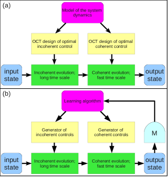
Figure 1: (Color online). Implementing complete density matrix controllability with (a) optimal control theory (OCT) and (b) learning control. In (a), methods of OCT and a theoretical model of the system dynamics are used to find optimal incoherent and coherent controls $n^{*}_{k}$ and $u^{*}(t)$. In (b), the objective $J=\|\rho_{T}-\rho_{\rm f}\|$, where $\rho_{T}$ is the output state, is measured (block with letter “M“) at the end of each iteration and the result is used to design a new control, ideally with better performance. The cycle is repeated until obtaining a satisfactory output.

If the quantum system is sufficiently simple and all its relevant parameters are known, then methods of optimal control theory (OCT) can be used to find optimal fields $n^{*}_{\omega}$ and $u^{*}(t)$ as shown on Fig. 1, subplot (a). If the system is complex and (or) some of its relevant parameters are unknown then various adaptive learning algorithms can be used to implement the proposed scheme for engineering arbitrary quantum states (Fig. 1, subplot (b)). In this case, the creation of a desired diagonal mixed state $\tilde{\rho}_{\rm f}$ during the first stage of the control scheme can be realized with learning algorithms PeRa06 . The second stage can be implemented using learning algorithms for coherent control JuRa92 . Learning algorithms were shown to be efficient for both cases and therefore they will be efficient when used in a successive combination as required in the proposed scheme.

III Complete density matrix controllability

Depending on a particular problem, various notions of controllability for quantum systems are used Altafini ; Ramakrishna ; Schirmer2002 ; Wu07 ; Brumer2008 ; Polack2009 , including unitary controllability, pure state, density matrix and observable controllability Schirmer2002 , and complete density matrix controllability Wu07 . Unitary controllability means the ability to produce with available controls any unitary evolution operator $U$. Density matrix controllability means the ability to transfer one into another arbitrary density matrices with the same spectrum (i.e., kinematically equivalent density matrices); a particular case is pure state controllability as the ability to transfer one into another arbitrary pure states. Complete density matrix controllability means the ability to steer any initial (pure or mixed) density matrix $\rho_{\rm i}$ into any (pure or mixed) final density matrix $\rho_{\rm f}$, irrespective of their relative spectra Wu07 . This notion is different from density matrix controllability Schirmer2002 , where only kinematically equivalent density matrices are required to be accessible one from another, and is the strongest among all degrees of state controllability for quantum systems; complete density matrix controllability of a quantum system implies in particular its pure state and density matrix controllability. The suggested scheme allows for transferring one into another arbitrary density matrices thereby approximately realizing complete density matrix controllability of quantum systems — the strongest possible degree of their state control.

IV All-to-one controls

An all-to-one control $c_{*}$ is a control which steers all initial states into one final state. Such controls can be optimal simultaneously for all initial states Wu07 and their importance is motivated by the following. Let $J(c)\equiv J(\rho_{T})$ be an arbitrary control objective determined by the system density matrix $\rho_{T}$ evolving from the initial state $\rho_{0}$ to the final time $T$ under the action of the control $c$ (e.g., $J={\rm Tr}\,[\rho_{T}O]$ for some Hermitian observable $O$ or $J=\|\rho_{T}-\rho_{\rm f}\|$). In general, optimal controls — controls minimizing the objective — are different for different initial states. However, if $c_{*}$ is an all-to-one control steering all states into a state $\rho_{\rm f}$ minimizing $J$, then $c_{*}$ will optimize the objective for any initial system state. While an abstract theoretical construction of all-to-one controls was provided Wu07 in terms of special Kraus maps whose definition is also provided below, their physical realizations has remained as an open problem. The proposed control scheme provides a physical realization of all-to-one controls and the corresponding Kraus maps for any pure or mixed state $\rho_{\rm f}$. The all-to-one property is achieved during the first stage, where $n^{*}_{\omega}$ produces the same density matrix $\tilde{\rho}_{\rm f}$ independently of the initial state.

The density matrix representing the state of an $n$-level quantum system is a positive, unit-trace $n\times n$ matrix. We denote by $\mathcal{M}_{n}=\mathbb{C}^{n\times n}$ the set of all $n\times n$ complex matrices, and by $\mathcal{D}_{n}:=\{\rho\in\mathcal{M}_{n}\,|\,\rho=\rho^{\dagger},\rho\geq 0,\mathrm{Tr}(\rho)=1\}$ the set of all density matrices. A map $\Phi:\mathcal{M}_{n}\to\mathcal{M}_{n}$ is positive if $\Phi(\rho)\geq 0$ for any $\rho\geq 0$ in $\mathcal{M}_{n}$. A map $\Phi:\mathcal{M}_{n}\to\mathcal{M}_{n}$ is completely positive (CP) if for any $l\in\mathbb{N}$ the map $\Phi\otimes\mathbb{I}_{l}:\mathcal{M}_{n}\otimes\mathcal{M}_{l}\to\mathcal{M}_{n}\otimes\mathcal{M}_{l}$ is positive ($\mathbb{I}_{l}$ is the identity map in $\mathcal{M}_{l}$). A CP map is trace preserving if $\mathrm{Tr}[\Phi(\rho)]=\mathrm{Tr}(\rho)$ for any $\rho\in\mathcal{M}_{n}$. Completely positive trace preserving maps are referred to as Kraus maps; they represent the reduced dynamics of quantum systems initially uncorrelated with the environment TarasovBook ; Kraus83 .

Any Kraus map $\Phi$ can be represented using the operator-sum representation (OSR) as $\Phi(\rho)=\sum_{i=1}^{l}K_{i}\rho K^{\dagger}_{i}$, where $\{K_{i}\}$ is a set of complex $n\times n$ matrices satisfying the condition $\sum_{i=1}^{l}K^{\dagger}_{i}K_{i}=\mathbb{I}_{n}$ to ensure trace preservation TarasovBook ; Kraus83 . The OSR is not unique: any Kraus map $\Phi$ can be represented using infinitely many sets of Kraus operators.

The all-to-one Kraus map for a given final state $\rho_{\rm f}=\sum_{i}p_{i}|\phi_{i}\rangle\langle\phi_{i}|$ is defined as a Kraus map $\Phi_{\rho_{\rm f}}$ steering all initial states into $\rho_{\rm f}$, i.e., such that $\Phi_{\rho_{\rm f}}(\rho)=\rho_{\rm f}$ for all $\rho\in{\cal D}_{n}$ Wu07 . If $\rho_{\rm f}$ is a density matrix maximizing a given objective $J$ and $c_{*}$ is a control producing the map $\Phi_{\rho_{\rm f}}$, then this control will be simultaneously optimal for all initial states, i.e., the same $c_{*}$ will maximize the objective for any initial system state. An OSR for a universally optimal Kraus map $\Phi_{\rho_{\rm f}}$ can be constructed by using $K_{ij}=\sqrt{p_{i}}|\phi_{i}\rangle\langle\phi_{j}|$ as the Kraus operators. Indeed, for any $\rho$, $\sum_{i,j=1}^{n}K_{ij}\rho K^{\dagger}_{ij}=\rho_{\rm f}$.

All-to-one Kraus maps were constructed theoretically in Wu07 . The two stage control scheme described in the present paper provides an approximate physical realization of all-to-one Kraus maps $\Phi_{\rho_{\rm f}}$ for all $\rho_{\rm f}$ (therefore any all-to-one Kraus map can be produced using this scheme) for generic systems unitary controllable on the fast with respect to $\tau_{\rm rel}$ time scale.

V Example: calcium atom

The scheme is illustrated below with an example of a two-level atom whose all relevant parameters are known and it is easy to analytically understand and visualize the controlled dynamics. We consider calcium upper and lower levels $\rm 4^{1}P$ and $\rm 4^{1}S$ as two states $|1\rangle$ and $|0\rangle$ of the two-level system. For this system the transition frequency is $\omega_{21}=4.5\times 10^{15}$ rad/s, the radiative lifetime $t_{21}=4.5$ ns, the Einstein coefficient $A_{21}=1/t_{21}\approx 2.2\times 10^{8}$ s^-1, and the dipole moment $\mu_{12}=2.4\times 10^{-29}$ C$\cdot$m Hilborn . The method works equally well for any initial and target states, we take for the sake of definiteness $\rho_{0}=|0\rangle\langle 0|$ and $\rho_{\rm f}=\frac{1}{4}|0\rangle\langle 0|+\frac{3}{4}|1\rangle\langle 1|$.

The system is generic, all its relevant parameters are known and we can analytically find optimal controls. The goal of the first (incoherent) stage is to prepare the mixture $\tilde{\rho}_{\rm f}=\frac{3}{4}|0\rangle\langle 0|+\frac{1}{4}|1\rangle\langle 1|$. This goal is realized by applying to the system incoherent radiation with spectral density satisfying $n_{\omega_{21}}=1/2$ during time $T$ of several magnitudes of decoherence time $t_{21}$; we choose $T=50$ ns. The goal of the second (coherent) stage is to rotate the state produced at the end of the first stage to transform it into $\rho_{\rm f}$. This goal can be realized for example by applying a resonant $\pi$-pulse $E(t)=E\cos(\omega_{12}t)$. Other methods of coherent control which produce the same unitary transformation can be used as well. The electric field amplitude which makes the Rabi frequency equal to the radiative decay rate is $E\approx 10^{3}$ V/m Hilborn . The proposed scheme requires the duration of the second stage to be significantly shorter that the decay time. This can be satisfied by choosing $E\gtrapprox 10^{4}$ V/m. We take resonant electromagnetic field $E(t)=E\cos(\omega_{12}t)$ of amplitude $E=10^{7}$ V/m acting on the system during the time interval $T_{\rm f}-T=1310$ fs. The Rabi frequency for the field of such amplitude is $\Omega_{\rm R}\approx 1/2320$ fs^-1, thus the field acts as a $\pi$-pulse transforming the state $\tilde{\rho}_{\rm f}$ into $\rho_{\rm f}$. The results of the numerical simulation are shown on Fig. 2. The time interval $1310$ fs is much less than $t_{21}$ and decoherence effects are negligible during the second stage. For illustrative purpose of better visualization of the trajectory during the second stage we provide in Fig. 3 simulation results for $E=10^{9}$ V/m and $T_{\rm f}-T=13.1$ fs. The method can be applied for producing arbitrary pure or mixed target density matrices from any pure or mixed initial state thereby implying complete density matrix controllability of this system.

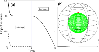
Figure 2: (Color online). Application of the control scheme for engineering a desired mixed state of two Ca energy levels. Subplot (a) shows the behavior of the objective vs. time during the two stages of the control. The timescale is not uniform, the duration of the first stage is $T=50$ ns and of the second stage is $T_{\rm f}-T=1310$ fs. Solid line is for $\|\rho_{t}-\rho_{\rm f}\|$ and dotted line for $\|\rho_{t}-\tilde{\rho}_{\rm f}\|$; the latter quantity almost completely vanishes during the first stage of the control. Subplot (b) shows the corresponding evolution of the Bloch vector. The initial system state corresponds to the south pole, the vertical blue line represents incoherent evolution during the first stage and the green line shows coherent rotations during the second stage under the action of resonant field of amplitude $E=10^{7}$ V/m. The evolved state approaches the target state indicated by the red marker.

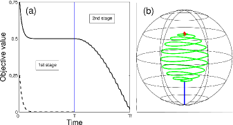
Figure 3: (Color online). The only difference from the description of Fig. 2 is that $E=10^{9}$ V/m and $T_{\rm f}-T=13.1$ fs.

References

- (1) D. J. Tannor and S. A. Rice, J. Chem. Phys. 83, 5013 (1985); A. P. Peirce, M. A. Dahleh, and H. Rabitz, Phys. Rev. A 37, 4950 (1988); A. G. Butkovskiy and Yu. I. Samoilenko, Control of Quantum-Mechanical Processes and Systems (Kluwer Academic Publishers, Dordrecht, Boston, 1990); S. A. Rice and M. Zhao, Optical Control of Molecular Dynamics (Wiley, New York, 2000); P. W. Brumer and M. Shapiro, Principles of the Quantum Control of Molecular Processes (Wiley-Interscience, 2003); M. Dantus and V. V. Lozovoy, Chem. Rev. 104, 1813 (2004); D. D’Alessandro, Introduction to Quantum Control and Dynamics (Chapman and Hall, 2007); D. Tannor, Introduction to Quantum Mechanics: A Time Dependent Perspective (University Science Press, Sausalito, 2007); V. S. Letokhov, Laser Control of Atoms and Molecules (Oxford University Press, USA, 2007); D. V. Zhdanov and V. N. Zadkov, Phys. Rev. A 77, 011401(R) (2008); C. Brif, R. Chakrabarti, and H. Rabitz, New J. Phys. 12, 075008 (2010); H. M. Wiseman and G. J. Milburn, Quantum Measurement and Control (Cambridge University Press, Cambridge, 2010).
- (2) A. Pechen and H. Rabitz, Phys. Rev. A 73, 062102 (2006).
- (3) R. Romano and D. D’Alessandro, Phys. Rev. A 73, 022323 (2006); Z. Yin et al., Phys. Rev. A 76, 062311 (2007); H. Schomerus and E. Lutz, Phys. Rev. A 77, 062113 (2008); W. Cui et al., Phys. Rev. A 77, 032117 (2008); S. G. Schirmer and X. Wang, Phys. Rev. A 81, 062306 (2009); F. O. Prado et al., Phys. Rev. Lett. 102, 073008 (2009); S. Pielawa et al., Phys. Rev. A 81, 043802 (2010); J. Paavola and S. Maniscalco, Phys. Rev. A 82, 012114 (2010); H. Zhong, W. Hai, G. Lu, and Z. Li, Phys. Rev. A 84, 013410 (2011).
- (4) H. M. Wiseman and G. J. Milburn, Phys. Rev. Lett. 70, 548 (1993); R. Vilela Mendes and V. I. Man’ko, Phys. Rev. A 67, 053404 (2003); A. Pechen et al., Phys. Rev. A 74, 052102 (2006); F. Shuang et al., Phys. Rev. A 78, 063422 (2008); A. E. B. Nielsen et al., Phys. Rev. A 79, 023841 (2009); C. Bergenfeldt and K. Mølmer, Phys. Rev. A 80, 043838 (2009); R. Ruskov et al., Phys. Rev. Lett. 105, 100506 (2010).
- (5) C. K. Law, J. H. Eberly, and B. Kneer, J. Mod. Optics 44, 2149 (1997).
- (6) V. E. Tarasov, J. Phys. A: Math. Gen. 35, 5207 (2002).
- (7) K. Vogel, V. M. Akulin, and W. P. Schleich, Phys. Rev. Lett. 71, 1816 (1993).
- (8) E. Bimbard, N. Jain, A. MacRae, and A. I. Lvovsky, Nature Photonics 4, 243 (2010).
- (9) S. Lloyd and L. Viola, Phys. Rev. A 65, 010101 (2001).
- (10) C. Altafini, J. Math. Phys. 44, 2357 (2003); C. Altafini, Phys. Rev. A 70, 062321 (2004).
- (11) F. Verstraete, M. M. Wolf, and J. I. Cirac, Nature Physics 5, 633 (2009).
- (12) F. Pastawski, L. Clemente, and J. I. Cirac, Phys. Rev. A 83, 012304 (2011).
- (13) S. Diehl, A. Micheli, A. Kantian, B. Kraus, H. P. Buchler, and P. Zoller, Nature Physics 4, 878 (2008).
- (14) J. T. Barreiro, P. Schindler, O. Gühne, T. Monz, M. Chwalla, C. F. Roos, M. Hennrich, and R. Blatt, Nature Physics 6, 943 (2010).
- (15) D. J. Tannor, R. Kosloff, and A. Bartana, Faraday Discuss. 113, 365 (1999); S. G. Schirmer, Phys. Rev. A 63, 013407 (2001).
- (16) R. Wu et al., J. Phys. A 40, 5681 (2007).
- (17) H.-P. Breuer and F. Petruccione, The Theory of Open Quantum Systems (Oxford University Press, Oxford, 2002).
- (18) V. E. Tarasov, Quantum Mechanics of Non-Hamiltonian and Dissipative Systems (Elsevier Science, 2008).
- (19) G. Lindblad, Commun. Math. Phys. 48, 119 (1976); V. Gorini, A. Kossakowski, and E. C. G. Sudarshan, J. Math. Phys. 17, 821 (1976).
- (20) E. B. Davies, Quantum Theory of Open Systems (Academic Press, London, 1976); S. Attal, A. Joye, C.-A. Pillet, Open Quantum Systems: The Markovian Approach (Springer, 2006).
- (21) H. Spohn and J. L. Lebowitz, Adv. Chem. Phys. 38, 109 (1978); H. Spohn, Rev. Mod. Phys. 53, 569 (1980).
- (22) L. Accardi and K. Imafuku, in QP–PQ: Quantum Probability and White Noise Analysis (World Scientific, Singapore, 2006), Vol. 19, p. 28.
- (23) V. Ramakrishna, M. V. Salapaka, M. Dahleh, H. Rabitz, and A. Peirce, Phys. Rev. A 51, 960 ̵͑(1995͒).
- (24) S. G. Schirmer, H. Fu, and A. I. Solomon, Phys. Rev. A 63, 063410 (2001).
- (25) N. Khaneja, R. Brockett, and S. J. Glaser, Phys. Rev. A 63, 032308 (2001).
- (26) L. Viola and S. Lloyd, Phys. Rev. A 58, 2733 (1998); K. Khodjasteh, D. Lidar, and L. Viola, Phys. Rev. Lett. 104, 090501 (2010).
- (27) R. Schmidt, A. Negretti, J. Ankerhold, T. Calarco, J. T. Stockburger, Optimal control of open quantum systems: cooperative effects of driving and dissipation, arXiv:1010.0940.
- (28) R. Alicki, private communications (2009).
- (29) R. S. Judson and H. Rabitz, Phys. Rev. Lett. 68, 1500 (1992).
- (30) S. G. Schirmer, A. I. Solomon, and J. V. Leahy, J. Phys. A: Math. Gen. 35, 4125 (2002).
- (31) L. Wu, A. Bharioke, and P. Brumer, J. Chem. Phys. 129, 041105 (2008).
- (32) T. Polack, H. Suchowski, and D. Tannor, Phys. Rev. A 79, 053403 (2009).
- (33) K. Kraus, States, Effects, and Operations (Springer, Berlin, 1983).
- (34) R. C. Hilborn, Am. J. Phys. 50, 982 (1982).