Reconstruction of Higgs bosons in the di-tau channel via 3-prong decay

Abstract:

We propose a method for reconstructing the mass of a particle, such as the Higgs boson, decaying into a pair of $\tau$ leptons, of which one subsequently undergoes a 3-prong decay. The kinematics is solved using information from the visible decay products, the missing transverse momentum, and the 3-prong $\tau$ decay vertex, with the detector resolution taken into account using a likelihood method. The method is shown to give good discrimination between a 125 GeV Higgs boson signal and the dominant backgrounds, such as $Z^{0}$ decays to $\tau\tau$ and $W^{\pm}$ plus jets production. As a result, we find an improvement, compared to existing methods for this channel, in the discovery potential, as well as in measurements of the Higgs boson mass and production cross section times branching ratio.

1 Introduction

The Standard Model Higgs boson – or something like it – has been found [1, 2] and the race is now on to determine its detailed properties. Of particular interest is the $\tau\tau$ decay channel, where, despite sensitivity to a signal comparable to that predicted in the Standard Model with $m_{h}\simeq 125$ GeV, only weak evidence somewhat below the Standard Model expectation has been seen [3, 4].

This may be evidence for physics beyond the Standard Model or it may be a statistical fluctuation. We should dearly like to get to the bottom of the mystery, but progress is slowed by a number of complications in the $h\rightarrow\tau\tau$ search channel.

One complication is the problem of triggering and identifying $\tau$ leptons, which decay in a variety of ways, some of which resemble common-or-garden QCD jets. A second is that, since a $\tau$ decay always involves one or more invisible neutrinos, it is only possible to reconstruct the resonance in an approximate way. A third is the problem of distinguishing $h\rightarrow\tau\tau$ signal events from the dominant backgrounds, namely $Z\rightarrow\tau\tau$ decays (which, moreover, lie nearby in $\tau\tau$ invariant mass) and production of QCD jets, with or without a $W$ boson, in which other leptons or jets are mistakenly identified as $\tau$ leptons.

The third issue, of distinguishing the signal from backgrounds, is compounded by the second issue, that we are a priori unable to reconstruct the invariant mass of the $\tau\tau$ pair. As a result, and as is readily apparent from the data shown in [5], the signal and backgrounds lie close to each other in distributions of the observables that are currently available to us. Not only does this increase the integrated luminosity required to be sure that an apparent signal is not a mere background fluctuation, but it also increases our vulnerability to systematic errors.

To be explicit, imagine a hypothetical limit in which we have a signal (the Higgs) that consists of a narrow peak in invariant mass, a background (the $Z$) that is also a narrow peak, but centred elsewhere, and additional backgrounds (like $W$ plus jets and QCD) that are approximately flat in invariant mass. The signals and backgrounds are otherwise roughly indistinguishable in their dynamics. Now, if the observables that we have available are uncorrelated with the invariant mass, then we are essentially reduced to counting events in order to try to discover the signal and our ability to do so is greatly limited by the total statistics available. We are, moreover, completely at the mercy of systematic uncertainties in the overall background normalization, which we have no way to measure in data. Even if we were able to make a discovery in this way, we could at most make one measurement of the signal properties (its overall size) and here too we would be exposed to the systematic uncertainty in the background normalization.

Conversely, if we find a way to reconstruct, more or less, the invariant mass, the first benefit is that we are no longer limited by the overall statistics, but rather by the number of signal and background events in a region of invariant mass of our choosing (near 125 GeV being the obvious choice for $h\rightarrow\tau\tau$). Moreover, we now have a clean separation between the signal and background and indeed between the different backgrounds themselves. This opens up the possibility of using the extra information to constrain the uncertainties on the background yields and shapes via data-driven techniques. Indeed, a simple sideband analysis would suffice, in which the $Z$ background is measured in a ‘control’ region near 90 GeV and the other backgrounds are measured in a control region away from the peaks near 90 GeV and 125 GeV. Finally, independent measurements of the signal mass and cross-section times branching ratio become possible.

Needless to say, the real situation is rather more complicated for $h\rightarrow\tau\tau$ at the LHC, with the current performance falling somewhere between the two extremes of perfect and imperfect mass resolution. Nevertheless, the basic principle remains the same: the more we are able to separate the signal and the different background components from each other, the less we shall find ourselves at the mercy of statistical and systematic uncertainties.

So, how could we reconstruct something like the $\tau\tau$ invariant mass? Several approximate methods or observables have previously been suggested in the literature (see, for example, [6, 7, 8, 9, 10, 11]). Some of these suffer from being rather poorly correlated with the invariant mass (some provide, for example, only an upper or lower bound on it), while others suffer from the fact that they turn out to be ill-defined for a significant fraction of events, with a consequent loss of statistics. As examples, the collinear approximation used in [10] fails for one in three events, whereas the observable used in [6, 11] does not exist for a similar fraction of events.

Here we wish to propose yet another method, which differs significantly in that we focus on the subset of events in which a $\tau$ lepton undergoes a 3-prong decay. This implies an immediate disadvantage in the form of a reduced number of signal events overall for a given integrated luminosity: a $\tau$ lepton has a branching ratio of 15 % for a 3-prong decay (of which 9.3 % are to $\pi^{-}\pi^{+}\pi^{-}\nu_{\tau}$ and 4.6 % are to $\pi^{-}\pi^{+}\pi^{-}\pi^{0}\nu_{\tau}$) [12], meaning that only 28 % of di-$\tau$ events feature at least one 3-prong decay. However, the hope is that this disadvantage is more than compensated by the advantages.

These advantages all stem from the fact that the presence of a 3-prong decay allows us to reconstruct the $\tau\tau$ invariant mass, if the invariant mass of the neutrino or neutrinos from the other $\tau$ decay is known. Thus, for hadronic decays of the other $\tau$, we can fully reconstruct events (up to a discrete ambiguity and in the absence of detector mismeasurements, both of which we shall deal with below); for leptonic decays of the other $\tau$, we are able to partially reconstruct events. As a result we hope to benefit from a reduced exposure to statistical and systematic uncertainties as argued above.

The extra kinematic information needed to reconstruct comes from the location of the secondary (3-prong $\tau$-decay) vertex: if one can measure with reasonable accuracy the impact parameter of each of the three charged tracks, defined as the shortest distance between the track and the primary vertex, then the intersection of these impact parameters gives the location of the secondary vertex.

Now, the location of the secondary vertex tells us the direction of the $\tau$ momentum; the mass-shell constraint for the $\tau$ then allows to reconstruct the magnitude of the $\tau$ momentum, up to a possible two-fold ambiguity. Given the measured missing transverse momentum, we are then able to reconstruct the momentum of the other $\tau$ (up to a further possible two-fold ambiguity), provided we know the invariant mass of the neutrino(s) produced in the other $\tau$ decay.

The reconstruction process just described can only be expected to work if things are well measured. For example, if they are not, we may end up with no real solutions to the kinematic constraints. We account for this by defining an ad hoc likelihood function in which we convolute the observed quantities with a function parameterizing the detector response. The maximum of this likelihood function is an event observable (albeit one with an obscure definition) and it is this observable that we propose to use for signal discrimination. The fact that we invoke a likelihood function also allows to deal with the unknown invariant mass of the two neutrinos produced in a leptonic $\tau$ decay: we marginalize with respect to the unknown invariant mass, including the matrix element for the $\tau$ decay.

Yet another advantage of focussing on 3-prong decays is that the fake backgrounds (coming from, e.g. W+ jets and QCD) will be reduced, as jets and other leptons are presumably less likely to fake a 3-prong decay (with a reconstructed secondary vertex) than they are to fake a generic hadronic tau or leptonic tau decay.

The outline of the paper is as follows. In the next Section, we describe the algebraic details of the reconstruction procedure. In Section 3, we present the results of our numerical simulations and in Section 4, we draw our conclusions.

2 The method

As described in the introduction, events are reconstructed using the decay vertex information. If one of the $\tau$ leptons decays to a 3-prong hadronic system and a $\tau$ neutrino, then the displacement $\mathbf{r}$ from the primary interaction point to the $\tau$ decay vertex should be measurable with useful precision.

Let us begin by considering the limit of perfect detector resolution. Denoting the energy, momentum and mass of the 3-prong decay products by $E_{j}$, $\mathbf{p}_{j}$ and $m_{j}$, respectively, and the angle between $\mathbf{r}$ and $\mathbf{p}_{j}$ by $\theta$, the momentum of that $\tau$ lepton can be reconstructed, with a twofold ambiguity, as $\mathbf{p}_{\tau}=p_{\tau}\mathbf{r}/|\mathbf{r}|$, where (neglecting the neutrino mass)

$$p_{\tau}=\frac{(m_{\tau}^{2}+m_{j}^{2})p_{j}\cos\theta\pm E_{j}\sqrt{(m_{\tau}^{2}-m_{j}^{2})^{2}-4m_{\tau}^{2}p_{j}^{2}\sin^{2}\theta}}{2(m_{j}^{2}+p_{j}^{2}\sin^{2}\theta)}\,.$$ (1)

The other $\tau$ lepton may decay either hadronically or leptonically, into a visible system $j^{\prime}$ (a hadronic jet or a charged lepton) and an invisible system $i^{\prime}$ (a $\tau$ neutrino or a pair of neutrinos). The transverse momentum of the invisible system is found from the missing transverse momentum, $\not{\mathbf{p}}_{T}$, and the reconstructed momentum of the first $\tau$ via

$$\mathbf{p}_{Ti^{\prime}}=\not{\mathbf{p}}_{T}+\mathbf{p}_{Tj}-\mathbf{p}_{T\tau}\,.$$ (2)

Given the invariant mass of the invisible system, $m_{i^{\prime}}=m_{\nu}=0$ for a hadronic and $m_{i^{\prime}}=m_{\nu\nu}\geq 0$ for a leptonic decay, one can then solve for the invisible longitudinal momentum, again with a twofold ambiguity:

$$p_{L{i^{\prime}}}=\frac{1}{\mu_{j^{\prime}}}\left(\alpha\,p_{Lj^{\prime}}\pm E_{j^{\prime}}\sqrt{\alpha^{2}-\mu_{i^{\prime}}\mu_{j^{\prime}}}\right)\,,$$ (3)

where

$$\mu_{i^{\prime}}=p_{T{i^{\prime}}}^{2}+m_{i^{\prime}}^{2}\,,\;\;\mu_{j^{\prime}}=p_{Tj^{\prime}}^{2}+m_{j^{\prime}}^{2}\,,\;\;\alpha=\frac{1}{2}(m_{\tau}^{2}-m_{j^{\prime}}^{2}-m_{i^{\prime}}^{2})+\mathbf{p}_{T{i^{\prime}}}\cdot\mathbf{p}_{Tj^{\prime}}\,.$$ (4)

The momentum of the second $\tau$ can now be reconstructed as $\mathbf{p}_{\tau^{\prime}}=\mathbf{p}_{i^{\prime}}+\mathbf{p}_{j^{\prime}}$, and hence the invariant mass of the $\tau\tau$ system, $m_{\tau\tau}$ is determined, up to a fourfold ambiguity.

Now consider a real detector and let $\mathbf{q}=(\mathbf{r},E_{j},\mathbf{p}_{j},\mathbf{p}_{j}^{\prime},\not{\mathbf{p}}_{T})$ correspond to the measured quantities. These do not coincide with their true values in an event, which we now denote by $\tilde{\mathbf{q}}$, but rather are shifted by amounts depending on the detector resolution, which we describe by a response function, $f(\mathbf{q},\tilde{\mathbf{q}})$. Then the likelihood, as a function of the true invariant mass $\tilde{m}_{\tau\tau}$, for an event with measured quantities $\mathbf{q}$, may be written as

$${\cal L}(\tilde{m}_{\tau\tau}|\mathbf{q})=\int d\tilde{\mathbf{q}}\,f(\mathbf{q},\tilde{\mathbf{q}})\,{\cal M}(\tilde{\mathbf{q}})\,\delta[\tilde{m}_{\tau\tau}-m_{\tau\tau}(\tilde{\mathbf{q}})]$$ (5)

where ${\cal M}(\tilde{\mathbf{q}})$ is the matrix-element squared for the decay and $m_{\tau\tau}(\tilde{\mathbf{q}})$ is the invariant $\tau\tau$ mass reconstructed from the true quantities $\tilde{\mathbf{q}}$ according to the recipe described above. Here ${\cal M}(\tilde{\mathbf{q}})$ should also include the jacobian factor relating the final-state phase space to the quantities $\tilde{\mathbf{q}}$. We find, in most cases, that including these effects gives, at best, a marginal improvement in the mass resolution. Indeed, some effects (such as the exponential distribution of the $\tau$-decay lifetimes), lead to large fluctuations in the likelihood integrand and hence to large errors in the numerical integration, worsening the mass resolution. Thus we do not include these effects, in general.

There is, however, one such effect which we do include. In the case of leptonic decay of the second $\tau$, the matrix elements also depend on the momenta of the two invisible neutrinos, and the right-hand side of eq. (5) should include an integration over their phase space, weighted by the expected distribution of the $\nu\nu$ invariant mass. This is conveniently expressed as $P(m_{\nu\nu}^{2})\,d\Phi_{\nu\nu}$, with

$$d\Phi_{\nu\nu}=\frac{d^{3}\mathbf{p}_{\nu\nu}}{2(2\pi)^{3}E_{\nu\nu}}\frac{d\Omega^{*}}{(4\pi)^{3}}dm_{\nu\nu}^{2}\,,$$ (6)

where $d\Omega^{*}$ is the element of solid angle in the $\nu\nu$ centre-of-mass frame and

$$P(m_{\nu\nu}^{2})=\frac{2}{m_{\tau}^{2}}\left(1-\frac{m_{\nu\nu}^{2}}{m_{\tau}^{2}}\right)^{2}\left(1+2\frac{m_{\nu\nu}^{2}}{m_{\tau}^{2}}\right)\,.$$ (7)

At each phase-space point, the value of $m_{\nu\nu}$ is then used, with this weight, for the reconstruction of the decay.

In the integral over the delta function in eq. (5), we include all real solutions to the equation $\tilde{m}_{\tau\tau}=m_{\tau\tau}(\tilde{\mathbf{q}})$. In contrast to [9], complex solutions should be discarded here, since they cannot correspond to true values for genuine $\tau\tau$ resonance events. Note, however, that measured values $\mathbf{q}$ that would correspond to complex values of $m_{\tau\tau}$ lying close to the real axis if reconstructed directly, which correspond to real solutions shifted slightly by detector resolution, will be included in the integration at neighbouring values of $\tilde{\mathbf{q}}$. For fake backgrounds, we often find that no nearby values of $\tilde{\mathbf{q}}$ lead to real solutions, allowing the event to be rejected.

We perform the integrations in eq. (5) by a Monte Carlo method similar to that adopted in [14], generating a large number of points $\tilde{\mathbf{q}}$ distributed around each measured point $\mathbf{q}$ according to a smearing function $f(\mathbf{q},\tilde{\mathbf{q}})$ deduced from detector simulations. The jet masses are generated according to certain probabilities that we describe in the Appendix. Each real solution $\tilde{m}_{\tau\tau}=m_{\tau\tau}(\tilde{\mathbf{q}})$ is entered into a histogram with the corresponding weight. Because the Monte Carlo method generates only a finite number of points, all histogram bins are given a small positive offset, to avoid multiplications by zero.

Since our likelihood function does not encode the matrix element in its entirety, we cannot expect to be able to make statistical inferences directly from it in the usual way. Doing so might lead, for example, to us wrongly rejecting the Standard Model Higgs boson hypothesis, or obtaining a biased measurement of its mass. Instead, we use our ad hoc likelihood function to define an event observable in the following way: for each event, we extract the smallest value of $\tilde{m}_{\tau\tau}$ that gives a local maximum of the event likelihood and define this to be the event value of the observable $m_{\mathrm{SV}}$. Our simulations suggest that this observable gives distributions for Higgs and $Z$ boson event samples whose peak locations provide a good determination of the corresponding boson mass, with small tails. In any case, the presence of such effects can be mitigated by comparing experimental distributions of observables to template Monte-Carlo samples, as we do in simulations of pseudo-experiments below.

3 Simulations and results

Our study is based on a sample from the Herwig++ event generator [15], version 2.52 [16] and corresponds to an integrated luminosity of 20 fb^-1, which is very similar to what has been achieved at the LHC by the end of 2012.

As regards the signal, recent Standard Model predictions for Higgs production at the LHC may be found in Ref. [17]. For a Higgs mass of 125 GeV, at a collision energy of 8 TeV, the expected total cross section is 19.52 pb in the gluon fusion channel and 1.58 pb in the vector boson fusion channel, with a probable uncertainty of around 10%. The predicted SM branching ratio for $\tau\tau$ decay, also given in Ref. [17], is 6.4%. Higgs production followed by $\tau\tau$ decay thus corresponds to a cross section of 1.34 pb.

For the $Z$ background, CMS [18] reports a flavour-averaged prediction of $\sigma(pp\rightarrow Z\rightarrow ll)=1.13$ nb and a measurement of 1.12 nb for the 8 TeV LHC. We take $\sigma(pp\rightarrow Z\rightarrow\tau\tau)=1.13$ nb. For the $W+j$ background, we use $\sigma(pp\rightarrow Wj)=2.15$ nb, taken from Herwig++.

All of our simulations are carried out at the parton level, without showering or hadronization effects, apart from hadronic tau decays which we simulate using Herwig++ [19]. The detector response was modelled as follows.

Firstly we assume identification efficiencies of 0.4 and 0.3 for the 1- and 3-prong hadronic taus, respectively [20]. The lepton identification efficiency is assumed to be 0.9 in our analysis. To estimate the number of $W+j$ events in which the jet mimics a 1- or 3-prong hadronic tau, we use the fake rates of 0.01 and 0.002 for 1- and 3-prong taus, respectively. These numbers are obtained from the simulation of $W+j$ events [21].

Secondly, we parameterize detector mismeasurements by smearing the energy component of jets and leptons with $\sigma(E)/E_{j}=0.5\,{\rm GeV}^{\frac{1}{2}}/\sqrt{E_{j}}$ and $\sigma(E)/E_{\ell}=0.05\,{\rm GeV}^{\frac{1}{2}}/\sqrt{E_{\ell}}$, respectively. For the missing transverse momentum, we smear each component with $\sigma_{x}=\sigma_{y}=5$ GeV.

For the $\tau$ decay vertex, the Monte-Carlo truth position is smeared by Gaussian distributions of widths $0.613\pm 0.008$ mm and $10.5\pm 0.2\,\mu$m, in the directions parallel and perpendicular to the 3-prong tau-jet, respectively. For jets that fake taus, we take the truth vertex position to be zero and then smear as above.

We then apply event selection cuts to purify the signal, for which we impose

$$p_{Tj}>20\,{\rm GeV},~{}~{}~{}~{}p_{Tj^{\prime}}>20\,{\rm GeV},~{}~{}~{}~{}\not{p}_{T}>20\,{\rm GeV}.$$ (8)

For the hadron-lepton mode, we further impose

$$m_{T}\equiv\sqrt{2|{\bf p}^{\ell}_{T}||{\not{\mathbf{p}}_{T}}|(1-\cos\Delta\phi)}<40\,{\rm GeV}$$ (9)

to reduce the background involving $W$s, where $\Delta\phi$ is the azimuthal difference between the lepton and the missing transverse momentum. The cross section for each process/channel after taking account of the efficiencies of (mis)identification and the selection cuts is listed in Table 1. We use the 3 prong-hadron (-lepton) channel for $m_{\mathrm{S}V}$ and the hadron-hadron (-lepton) channel for $m_{\mathrm{v}is}$ and $m_{\mathrm{e}ff}$.

	3pr-had	3pr-lep	had-had	had-lep
$H$	6.3	5.7	17.2	28.5
$Z$	528.8	416.5	1451.4	2036.0
$Wj$	50.5	32.4	135.3	161.9

Table 1: The cross section times efficiency of each process/channel in fb.

In Figure 1 we compare the signal and background distributions of our variable $m_{\mathrm{SV}}$ with the existing variables $m_{\mathrm{eff}}$ and $m_{\mathrm{vis}}$. $m_{\mathrm{vis}}$ is simply the invariant mass of the visible products of both $\tau$ decays, while $m_{\mathrm{eff}}$ includes the missing transverse momentum (an explicit definition may be found in [10]). We show results for the lepton-hadron modes and hadron-hadron modes separately.

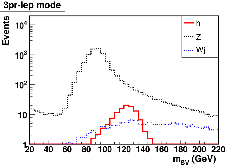
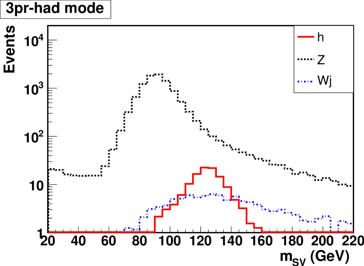
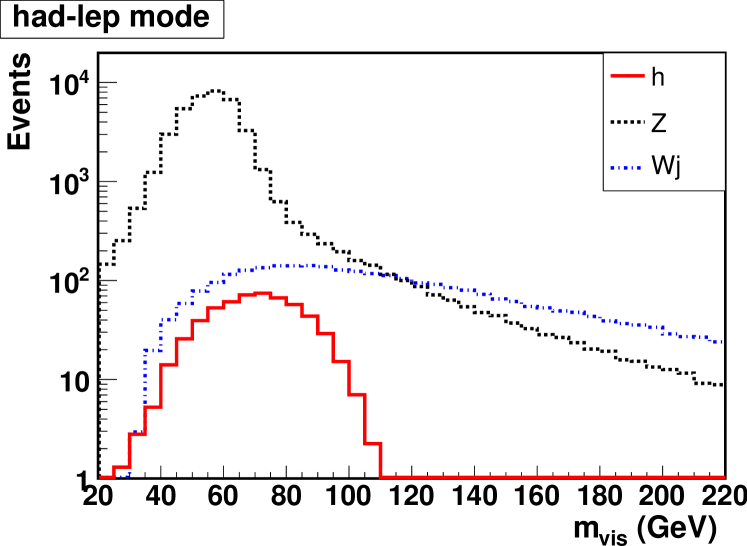
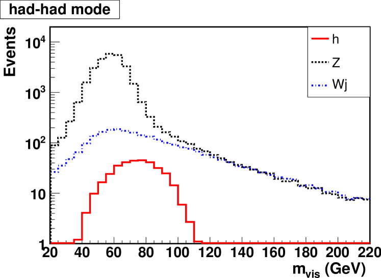
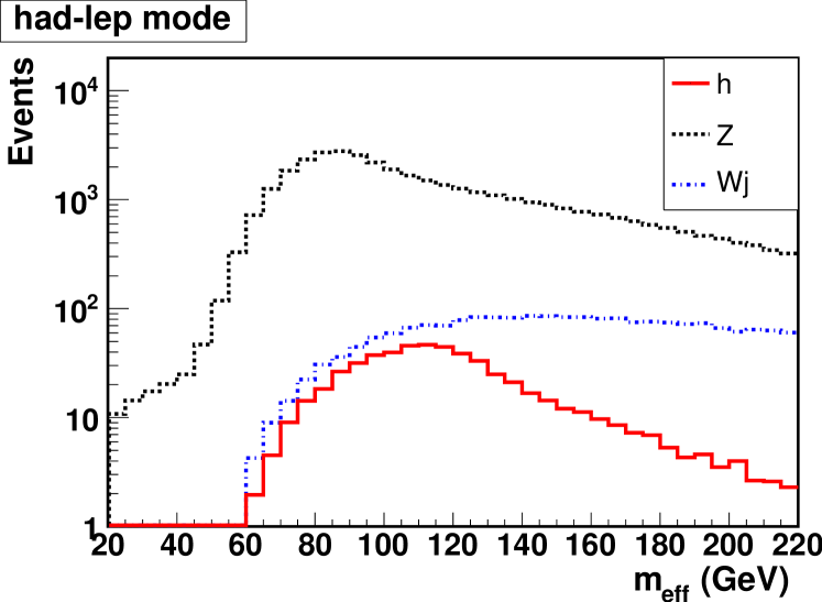
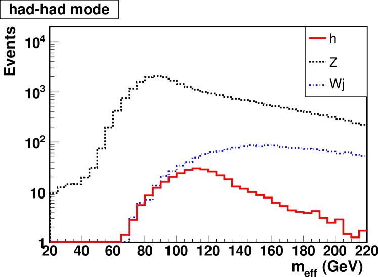
Figure 1: Signal and background distributions of $m_{\mathrm{SV}}$ (top), $m_{\mathrm{vis}}$ (centre) and $m_{\mathrm{eff}}$ (bottom), for an integrated luminosity of 20 fb^-1 at the 8 TeV LHC, for $m_{h}=125$ GeV. Left: lepton-hadron modes; right: hadron-hadron modes.

The better separation between signal and backgrounds that we expected to obtain using $m_{\mathrm{SV}}$ is clear to see in the Figure. Indeed, $m_{\mathrm{vis}}$ has distributions for the Higgs signal and $Z$ background which are strongly peaked, but the two peaks sit on top of each other. $m_{\mathrm{eff}}$ incorporates extra information in the form of the missing transverse momentum, and slightly increases the separation between the maxima of the Higgs and $Z$ boson peaks, but at the cost of introducing large tails (from the smearing of the missing transverse momentum measurement). As a result, the Higgs signal is easily hidden in the large tail of the $Z$ background. Moreover, the shapes of all components become similar, making discrimination difficult when the overall normalizations are uncertain. In contrast $m_{\mathrm{SV}}$ provides a good separation between the narrow Higgs and $Z$ boson peaks, which appear at the true mass values. These peaks are, furthermore, very different in shape from the continuum $W+$ jet background.

To see how well each variable can reconstruct the resonance, we list the peak location of the each variable’s distribution and the input mass of the resonance in Tables 3 and 3 in the hadron-hadron and hadron-lepton modes, respectively. The pure $Z\to\tau\tau$ and $h\to\tau\tau$ samples with several Higgs masses are used. The peak location is calculated as the weighed average of the three highest bins. The error is estimated by using 10 independent samples. The tables show clearly that $m_{\mathrm{SV}}$ reconstructs the masses of resonances very well compared to the other variables. Although this correlation is not the basis of our method for mass determination, it helps to separate the signal from the background.

Another remark is that the $S/B$ for the $W+$ jet background is better for $m_{\mathrm{SV}}$, as can be seen from Fig. 1. This is because a fraction of the $W+$ jet background events do not produce real solutions. The fact that the tau mass is much smaller than the typical momentum scale of the reconstructed objects (jets and leptons) implies that the neutrino momenta are inferred to be very close to those objects (see e.g. Eq. (1)). However the direction of this inferred momentum tends to conflict with the direction of the observed missing transverse momentum, since the neutrino from the $W$ decay is generally not collimated with respect to those objects, leading to no real solution.

Nevertheless, it is also apparent that the statistics available using $m_{\mathrm{SV}}$ are lower than for the other variables, even in the region of maximum signal. We need, therefore, to make a quantitative comparison of the three variables. To do so, we generate distributions of them (for $m_{h}=125$ GeV signal and backgrounds) in ten pseudo-experiments, each corresponding to an integrated luminosity of 20 fb^-1 of 8 TeV LHC data. Each pseudo-experiment is then compared to template model distributions with different values of $m_{h}$ and with different normalization factors $f_{h}$, $f_{W}$, and $f_{Z}$ for the Higgs signal and $W+j$ and $Z$ backgrounds, respectively. (The values $f_{h,W,Z}=1$ correspond to the leading order Monte-Carlo prediction.) Allowing the model distribution normalizations to float in this way allows us not only to take into account some of the most important systematic effects (arising from the uncertainties in the luminosity, the Monte-Carlo predictions, and data-driven extrapolations), but also provides a means to measure the cross-section times branching ratio for Higgs production followed by decay to $\tau\tau$.

	$Z$(91)	$h$(119)	$h$(125)	$h$(131)
$m_{\rm SV}$	$92.10\pm 0.01$	$117.81\pm 0.73$	$124.75\pm 0.75$	$130.84\pm 1.00$
$m_{\rm eff}$	$89.97\pm 0.02$	$110.55\pm 1.09$	$115.12\pm 1.19$	$115.12\pm 1.19$
$m_{\rm vis}$	$60.27\pm 0.01$	$73.87\pm 0.84$	$77.82\pm 1.05$	$78.42+-0.98$

Table 2: Peak position vs. input mass in the hadron-hadron mode. The numbers in the parentheses are the input mass of the bosons. Pure background and signal samples are used.

	$Z$(91)	$h$(119)	$h$(125)	$h$(131)
$m_{\rm SV}$	$91.54\pm 0.40$	$116.12\pm 0.82$	$122.15\pm 0.84$	$129.33\pm 0.68$
$m_{\rm eff}$	$89.90\pm 0.02$	$108.64\pm 1.12$	$113.27\pm 0.96$	$116.38\pm 1.20$
$m_{\rm vis}$	$59.87\pm 0.01$	$70.82\pm 0.83$	$73.59\pm 0.77$	$75.52\pm 1.28$

Table 3: Peak position vs. input mass in the hadron-lepton mode. The numbers in the parentheses are the input mass of the bosons. Pure background and signal samples are used.

We make a cut on the observable of interest itself, so as to maximize its discovery potential. Roughly speaking, this cut selects the region that contains the bulk of the signal events for that observable. Thus we choose $m_{\mathrm{SV}}\in[110,150]$ GeV, $m_{\mathrm{vis}}\in[75,110]$ GeV, and $m_{\mathrm{eff}}\in[100,150]$ GeV.

We then compute, for each pseudo-experiment, a binned Poisson log-likelihood, $\log\mathcal{L}=\Sigma_{i}\log\mathcal{L}^{P}\left(n^{\mathrm{trial}}_{i};x_{i}\right)$, where $n^{\mathrm{trial}}_{i}$ is the number of events observed in histogram bin $i$ in a given pseudo-experiment and $x_{i}=x_{i}(m_{h},f_{h},f_{Z},f_{W})$ is the number of events expected in a given model, parameterized by $m_{h},f_{h},f_{Z},f_{W}$.

To assess the discovery potential, we then compute the difference in log-likelihood between models with and without a Higgs signal. In the model without a signal, we maximize the log-likelihood with respect to $f_{Z},$ and $f_{W}$, whereas in the model with a signal, we additionally maximize with respect to $m_{h}$ and $f_{h}$. In Fig. 2, we show $-2$ times the difference in log-likelihood for the three variables. The centre of each bar shows the mean value over trials, while the width of each bar gives the root-mean-square deviation over trials.

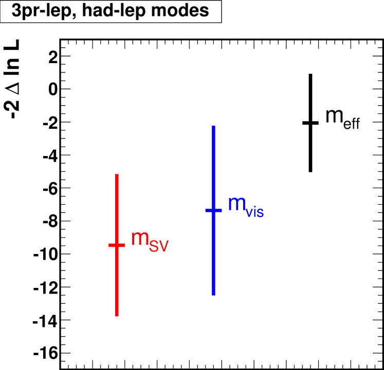
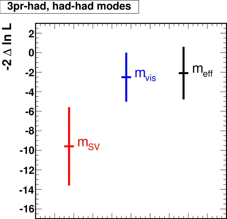
Figure 2: Discovery potential using $m_{\mathrm{SV}}$, compared to $m_{\mathrm{eff}}$ and $m_{\mathrm{vis}}$, for lepton-hadron (left) and hadron-hadron (right) modes, for an integrated luminosity of 20 fb^-1 at the 8 TeV LHC. The centre of each bar shows the mean value over trials, while the width of each bar gives the root-mean-square deviation.

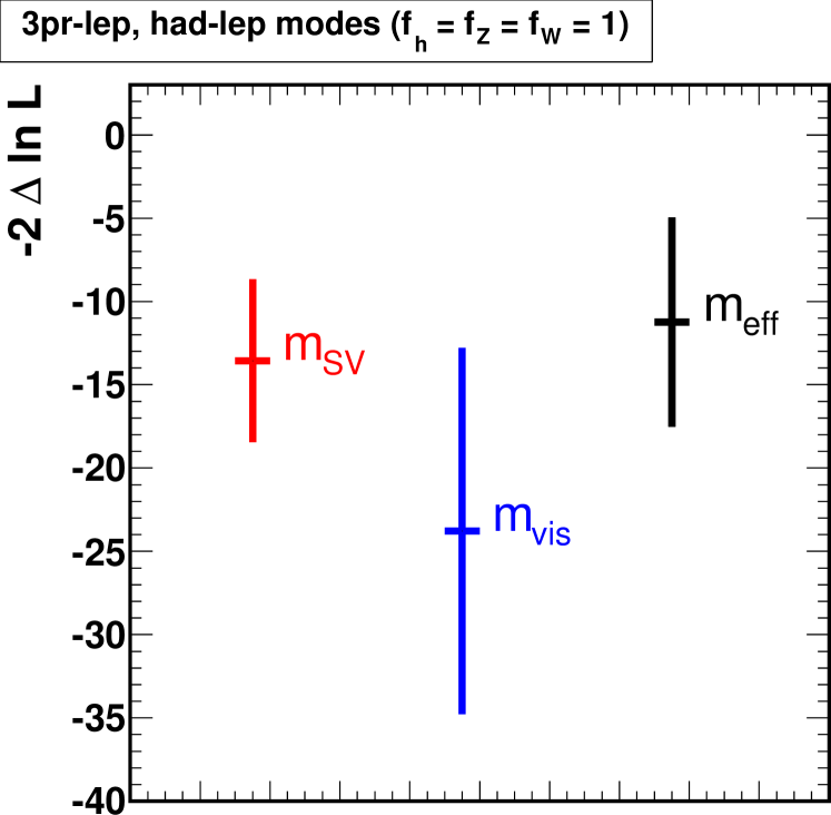
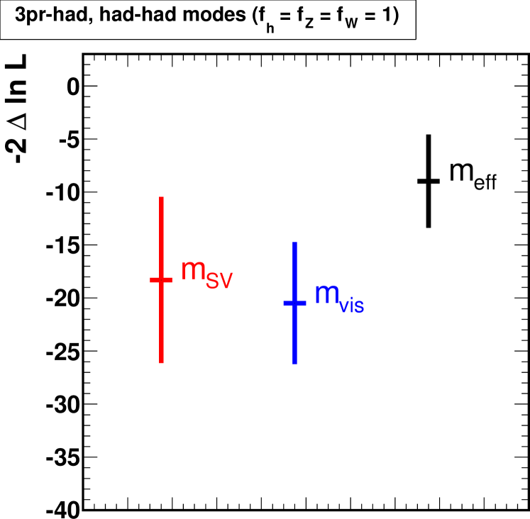
Figure 3: The same as Fig. 2, however $f$s are fixed at 1 in the likelihood calculation.

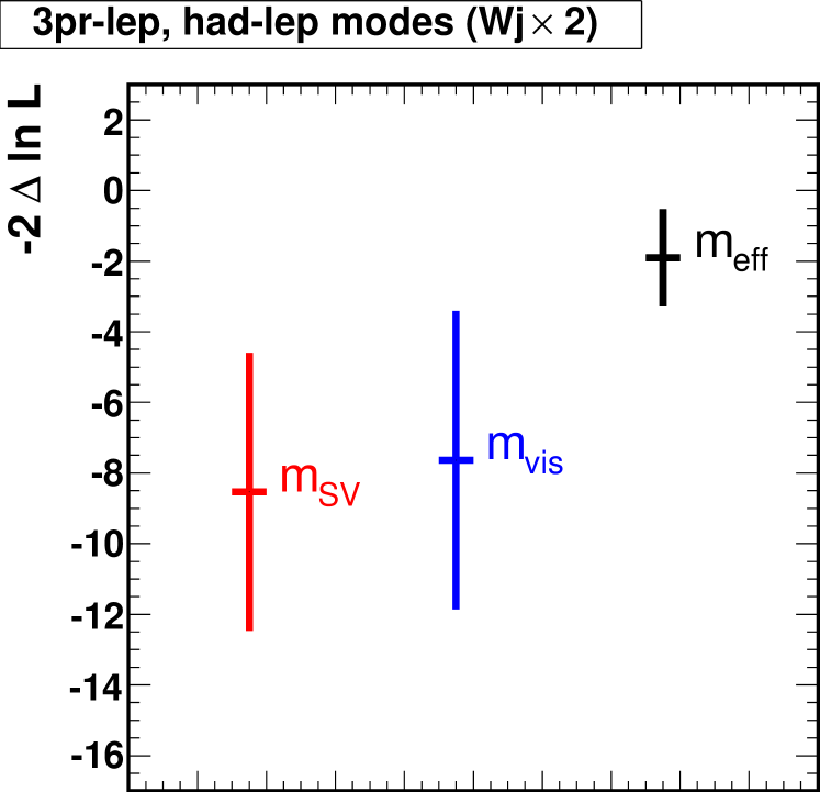
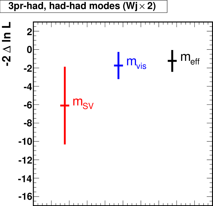
Figure 4: The same as Fig. 2, however the analysis uses a $W+j$ background sample which is twice as large as the expected one.

We observe a significant improvement using $m_{\mathrm{SV}}$ in the hadron-hadron channel, along with a more modest improvement (compared to $m_{\mathrm{vis}}$) in the leptonic channel. The different performances of $m_{\mathrm{vis}}$ in hadron-lepton and hadron-hadron modes can be understood from the distributions in Fig. 1. Unlike the hadron-lepton mode, the $m_{\mathrm{vis}}$ distribution in the hadron-hadron mode shows that both $Z$ and $W+j$ backgrounds as well as the signal have falling shapes in the signal region $m_{\mathrm{vis}}\in[75,110]$ GeV. This suggests that in the hadron-hadron mode, fitting the signal + background distribution with only the $Z$ and $W+j$ backgrounds by floating $f_{Z}$ and $f_{W}$ can be more possible compared to the hadron-lepton mode. This feature can be seen explicitly in Fig. 3, which show the same likelihoods as in Fig. 2 but with the $f$s fixed at 1. Floating the $f$s brings significant degradation for $m_{\mathrm{vis}}$ in the hadron-hadron mode.

The absolute values of the discovery significance are exaggerated, since we have neglected sub-dominant backgrounds and many uncertainties, but the relative performance of the different variables should be meaningful.

We have estimated the size of $W+j$ background using the reported tau fake rates in $W+j$ events. The tau fake rate is generally dependent on the tau identification algorithm and the jet $p_{T}$. To check the robustness of our result, in Fig. 4 we show the same discovery potential plots as Fig. 2 but containing a $W+j$ background twice as large as the one in Fig. 2. The discovery potentials are degraded slightly but the qualitative features are unchanged.

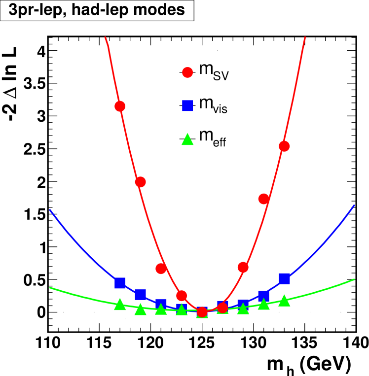
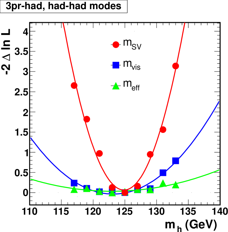
Figure 5: The log-likelihood function near $m_{h}=125$ GeV obtained using the $m_{\mathrm{SV}}$, $m_{\mathrm{eff}}$ and $m_{\mathrm{vis}}$ distributions, for lepton-hadron (left) and hadron-hadron (right) modes, for an integrated luminosity of 20 fb^-1 at the 8 TeV LHC.

	$m_{\rm SV}$	$m_{\rm vis}$	$m_{\rm eff}$
had-lep	4.7	11.0	23.3
had-had	4.7	11.8	23.1

Table 4: Uncertainty in the Higgs boson mass (in GeV), as measured $m_{\rm SV}$, $m_{\mathrm{eff}}$ and $m_{\mathrm{vis}}$ distributions, for lepton-hadron and hadron-hadron modes, for an integrated luminosity of 20 fb^-1 at the 8 TeV LHC.

To assess the expected resolution in the Higgs mass measurement, we first show, in Fig. 5, the variation in $-2\log\mathcal{L}$, averaged over pseudo-experiments, for values of the model Higgs mass, $m_{h}$, in the neighbourhood of 125 GeV, after maximizing $\mathcal{L}$ with respect to $f_{h},f_{Z}$, and $f_{W}$. In the figure, we have placed the minimum of $-2\log\mathcal{L}$ at height zero. Because the pseudo-experimental data and templates are prepared in the same way, we cannot estimate any biases that might occur when each variable is used to determine the mass from real data. However, for each variable, we can estimate the precision of the mass measurement from a quadratic fit to the log-likelihood. The resulting fractional uncertainties are shown in Table. 4 and are seen to be much smaller for $m_{\mathrm{SV}}$ than for the other two observables, in both hadron-hadron and lepton-hadron modes. This is easily explained by the fact that the Higgs signal peak is sharpest for $m_{\mathrm{SV}}$. For the measurement of the product of the production cross section and the branching ratio for the decay, the procedure is exactly analogous, except that now we vary $f_{h}$, after maximizing with respect to $m_{h}$. The resulting fit and fractional uncertainties are shown in Fig. 6 and Table 5, respectively. Again, there is always an improvement when using $m_{\mathrm{SV}}$. For $m_{\mathrm{vis}}$, the difference in resolution between the hadron-lepton and hadron-hadron modes can be blamed on different shapes in the $W+j$ background in these modes, as we have discussed earlier in the connection with the different discovery potentials for $m_{\mathrm{vis}}$ between these modes.

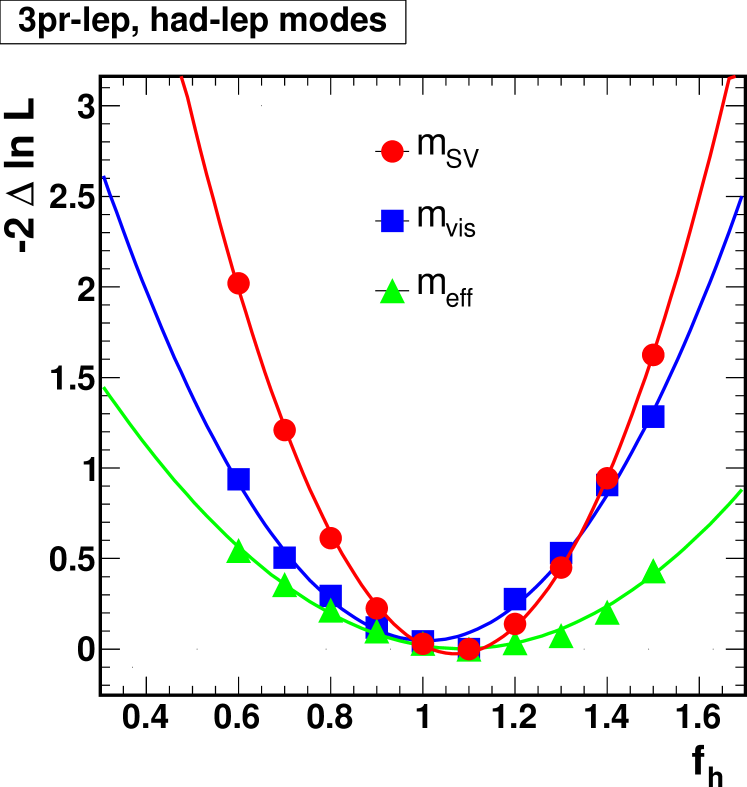
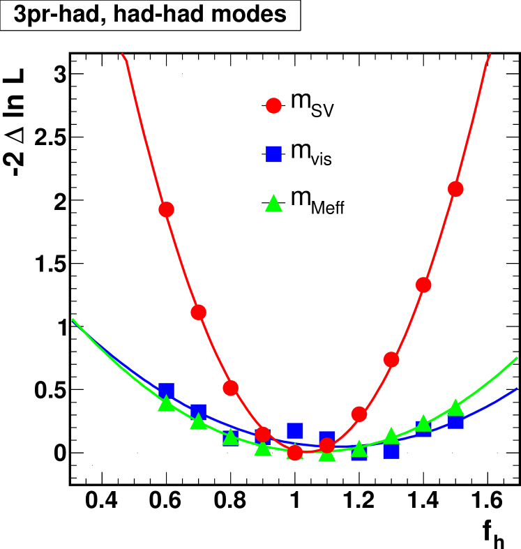
Figure 6: The log-likelihood as a function of the signal strength $f_{h}$, obtained using the $m_{\mathrm{SV}}$, $m_{\mathrm{eff}}$ and $m_{\mathrm{vis}}$ distributions, for lepton-hadron (left) and hadron-hadron (right) modes, for an integrated luminosity of 20 fb^-1 at the 8 TeV LHC. $f_{h}=1$ corresponds to the truth value.

	$m_{\rm SV}$	$m_{\rm vis}$	$m_{\rm eff}$
had-lep	0.33	0.44	0.65
had-had	0.32	0.93	0.73

Table 5: Resolution for measurement of the production cross section times branching ratio for $pp\rightarrow h\rightarrow\tau\tau$ normalized by the leading order prediction using $m_{\mathrm{SV}}$, compared to $m_{\mathrm{eff}}$ and $m_{\mathrm{vis}}$, for lepton-hadron (left) and hadron-hadron (right) modes, for an integrated luminosity of 20 fb^-1 at the 8 TeV LHC.

4 Conclusions

As shown in Figs. 2-6 and Tables 4-5, our simulations suggest that a significant improvement in discovery potential, Higgs boson mass resolution, and measurement of production cross section times branching ratio can be obtained by focussing on 3-prong $\tau$ decays. The performance of $m_{\mathrm{SV}}$ is roughly comparable irrespective of whether the other $\tau$ meson decays leptonically or hadronically, leading to greater gains in the hadron-hadron channel, where the other observables perform more poorly. One possible reason for this is that the detector resolution is invariably poorer in this channel, in which final-state leptons are replaced by jets. Thus the performance of $m_{\mathrm{vis}}$ and $m_{\mathrm{eff}}$ is degraded. However, these events are also fully reconstructible using the vertex information, in the absence of smearing. As a result, the likelihood that defines the observable $m_{\mathrm{SV}}$ is able to correct for the extra smearing to a certain extent, by insisting that the unsmeared quantites consistently reconstruct the event.

The gains are greatest for the mass measurement, which is perhaps not surprising since our method provides a means to reconstruct the mass whilst partially correcting for the uncertainties that are introduced by the detector resolution.

The results of our simulations are encouraging, but they should be taken with a pinch of salt. The simulations themselves are rudimentary, and we have only performed a comparison with the basic variables $m_{\mathrm{eff}}$ and $m_{\mathrm{vis}}$. Both collaborations now employ more sophisticated likelihood-based analyses. Unfortunately the full details of these have not been made public, so it is difficult for us to make a fair comparison. CMS do say that their likelihood method gives a Higgs mass resolution of around 21$\%$ compared to 24$\%$ using mvis [22].

We have also not made a full study of the backgrounds, of which many are relevant for this search. However, the two backgrounds we did consider are very different in their nature (one being a genuine, resonant background and the other being a fake, continuum background). We hope therefore, that the other backgrounds will be similar to one or other of these in their behaviour. The recent CMS results suggest, moreover, that our two backgrounds are the dominant ones in the signal region in most of the $\tau\tau$ sub-channels (along with pure jets, which we expect to be similar to $W+$jets).

Finally, we have only considered the most obvious systematic effect, namely the uncertainty associated with the normalization of the signal and backgrounds. Nevertheless, our qualtitative argument that a better mass reconstruction gives a better separation between the signal and the different backgrounds, means that many systematic uncertainties are expected to be reduced.

We hope, at least, that our qualitative arguments and quantitative simulations are enough to convince the collaborations to explore the suitability of this method. Even if it then turns out that a significant improvement is not obtained using our method alone, we remark that an overall improvement can still be expected if it is combined with existing approaches. Our method is complementary and, as is clear from Fig 7, the observable we extract is not strongly correlated with the existing variables $m_{\mathrm{eff}}$ and $m_{\mathrm{vis}}$. It thus provides independent information and may be used to increase the significance of searches in the $\tau\tau$ channel.

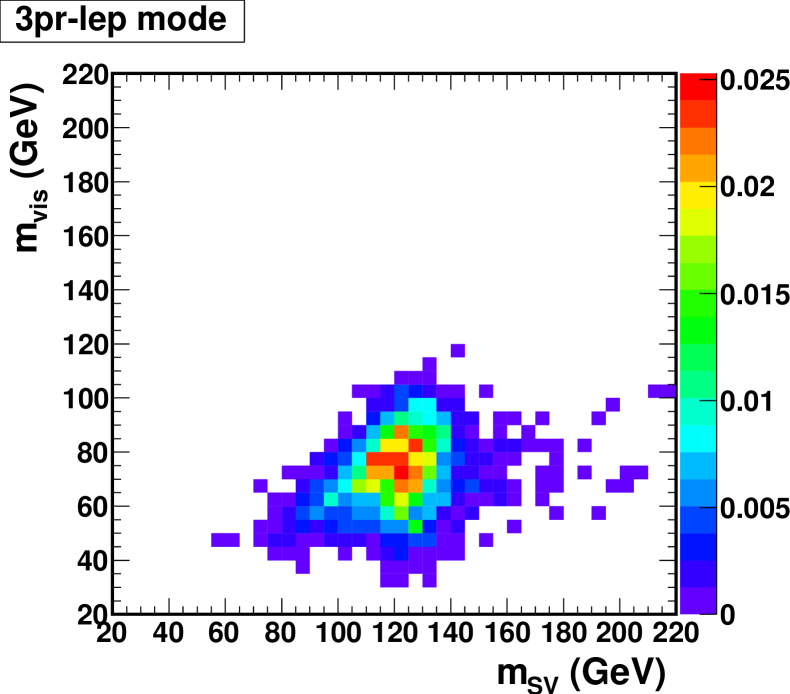
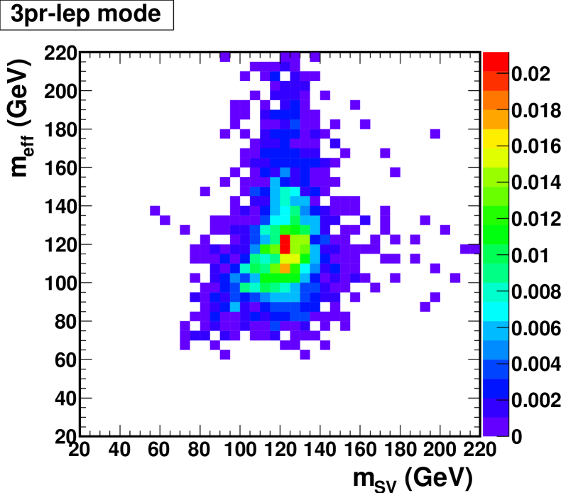
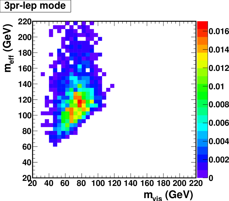
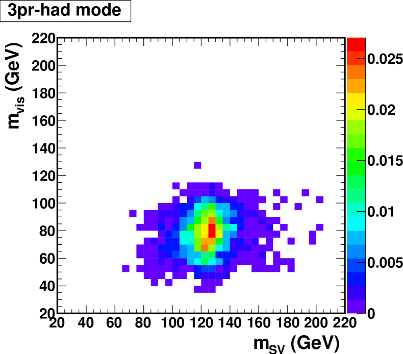
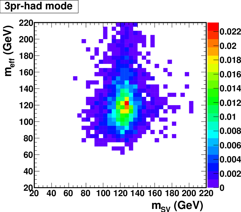
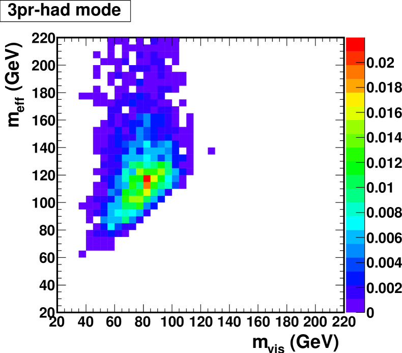
Figure 7: Correlation between $m_{\mathrm{SV}}$, $m_{\mathrm{eff}}$ and $m_{\mathrm{vis}}$, for the Higgs signal, for lepton-hadron (left) and hadron-hadron (right) modes.

Our simulations apply to the current 8 TeV run and our hope is that application of our method to data being produced now will allow us to clear up the mystery of the observed deficit of $h\rightarrow\tau\tau$ decays. Nevertheless, we expect our method to become even more relevant in the subsequent stages of the LHC programme. For one thing, the method is limited by statistics, but gains in reducing systematic uncertainties. It is the latter that will limit our ultimate ability to make precision measurements of the Higgs sector at the LHC. What is more, both ATLAS and CMS are planning upgrades or replacements of their vertex detectors, with an improvement of a factor of a few expected in the vertex resolution. The associated improvement in the $\tau\tau$ mass reconstruction using our method should reduce the uncertainties even further.

Appendix A The treatment of jet masses

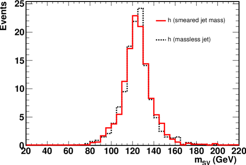
Figure 8: Comparison between two treatments of jet masses. The red solid histogram uses jet masses smeared by the Gaussian distributions, whilst the black dashed histogram uses massless jets. The $h\to\tau\tau$ events in the hadron-hadron mode are used.

As we discussed in section 2, in evaluating the likelihood function (5), we generate a large number of points ${\bf\tilde{q}}$ in which the jet energy is smeared, as well as the other observables, according to the detector resolution. The magnitude of the jet momentum is then calculated as $p_{j}=\sqrt{E_{j}^{2}-m_{j}^{2}}$, where $m_{j}$ is the jet mass. We generate the jet mass according to the following probabilities:

$$P_{\rm 1pr}(m_{j})=G(m_{j};m_{\rho},\sigma_{\rho})\cdot(1-R_{\tau\to\pi\nu})+\delta(m_{j}-m_{\pi})\cdot R_{\tau\to\pi\nu},$$ (10)

for the 1-prong tau-jet and

$$P_{\rm 3pr}(m_{j})=G(m_{j};m_{a},\sigma_{a}),$$ (11)

for the 3-prong tau-jet, where $R_{\tau\to\pi\nu}$ is the $BR(\tau\to\pi\nu)$ divided by the branching ratio of inclusive 1-prong tau decays and $G(x;\mu,\sigma)$ is Gaussian probability distribution with mean value $\mu$ and standard deviation $\sigma$. We took $m_{\rho}=775$ MeV, $\sigma_{\rho}=90$ MeV, $m_{a}=1230$ MeV and $\sigma_{a}=160$ MeV in our analysis.

We have checked that the treatment of the jet mass does affect the frequency of finding real solutions in the likelihood evaluation, but does not affect much the overall shape of the likelihood function. Thus, $m_{\rm SV}$ is rather robust against variation of the jet mass. To demonstrate this, we show two $m_{\rm SV}$ distributions for the $h\to\tau\tau$ events in the hadron-hadron channel in Figure 8, where one uses the jet mass described above and the other uses massless jets, with $P_{\rm 1pr}(m_{j})=P_{\rm 3pr}(m_{j})\propto\delta(m_{j})$. As can be seen, the two distributions are very similar.

References

- [1] ATLAS Collaboration, G. Aad et al., “Observation of a new particle in the search for the Standard Model Higgs boson with the ATLAS detector at the LHC,” Phys.Lett. B716 (2012) 1–29, arXiv:1207.7214 [hep-ex].
- [2] CMS Collaboration, S. Chatrchyan et al., “Observation of a new boson at a mass of 125 GeV with the CMS experiment at the LHC,” Phys.Lett. B716 (2012) 30–61, arXiv:1207.7235 [hep-ex].
- [3] ATLAS Collaboration, K. Einsweiler, “ATLAS Status Report on SM Higgs Search/Measurements,”. Talk presented at Hadron Collider Physics Symposium 2012 (HCP 2012).
- [4] CMS Collaboration, C. Paus, “Latest on the Higgs from CMS,”. Talk presented at Hadron Collider Physics Symposium 2012 (HCP 2012).
- [5] CMS Collaboration, “Search for the standard model Higgs boson decaying to tau pairs,”. CMS-PAS-HIG-12-043.
- [6] R. K. Ellis, I. Hinchliffe, M. Soldate, and J. J. van der Bij, “Higgs Decay to tau+ tau-: A Possible Signature of Intermediate Mass Higgs Bosons at the SSC,” Nucl. Phys. B297 (1988) 221.
- [7] CMS Collaboration, “Search for Neutral Higgs Boson Production and Decay to Tau Pairs,”. CMS-PAS-HIG-10-002.
- [8] A. Elagin, P. Murat, A. Pranko, and A. Safonov, “A New Mass Reconstruction Technique for Resonances Decaying to di-tau,” Nucl.Instrum.Meth. A654 (2011) 481–489, arXiv:1012.4686 [hep-ex].
- [9] B. Gripaios, K. Sakurai, and B. Webber, “Polynomials, Riemann surfaces, and reconstructing missing-energy events,” JHEP 1109 (2011) 140, arXiv:1103.3438 [hep-ph].
- [10] A. J. Barr, S. T. French, J. A. Frost, and C. G. Lester, “Speedy Higgs boson discovery in decays to tau lepton pairs : htau,tau,” JHEP 1110 (2011) 080, arXiv:1106.2322 [hep-ph].
- [11] A. J. Barr, B. Gripaios, and C. G. Lester, “Finding Higgs bosons heavier than 2 in dileptonic W-boson decays,” Phys.Lett. B713 (2012) 495–499, arXiv:1110.2452 [hep-ph].
- [12] Particle Data Group Collaboration, C. Amsler et al., “Review of particle physics,” Phys. Lett. B667 (2008) 1–1340.
- [13] ATLAS Collaboration, G. Aad et al., “Expected Performance of the ATLAS Experiment - Detector, Trigger and Physics,” arXiv:0901.0512 [hep-ex].
- [14] K. Kawagoe, M. M. Nojiri, and G. Polesello, “A new SUSY mass reconstruction method at the CERN LHC,” Phys. Rev. D71 (2005) 035008, arXiv:hep-ph/0410160.
- [15] M. Bahr et al., “Herwig++ Physics and Manual,” Eur. Phys. J. C58 (2008) 639–707, arXiv:0803.0883 [hep-ph].
- [16] S. Gieseke et al., “Herwig++ 2.5 Release Note,” arXiv:1102.1672 [hep-ph].
- [17] LHC Higgs Cross Section Working Group Collaboration, S. Dittmaier et al., “Handbook of LHC Higgs Cross Sections: 1. Inclusive Observables,” arXiv:1101.0593 [hep-ph].
- [18] CMS Collaboration, “W and Z inclusive cross sections at 8 TeV,”. SMP-PAS-12-011.
- [19] D. Grellscheid and P. Richardson, “Simulation of Tau Decays in the Herwig++ Event Generator,” arXiv:0710.1951 [hep-ph].
- [20] ATLAS Collaboration, G. Aad et al., “Measurement of the Z to tau tau Cross Section with the ATLAS Detector,” Phys.Rev. D84 (2011) 112006, arXiv:1108.2016 [hep-ex].
- [21] CMS Collaboration, “Performance of tau-lepton reconstruction and identification in CMS,” JINST 7 (2012) P01001, arXiv:1109.6034 [physics.ins-det].
- [22] CMS Collaboration, S. Chatrchyan et al., “Search for Neutral MSSM Higgs Bosons Decaying to Tau Pairs in pp Collisions at sqrt(s)=7 TeV,” Phys. Rev. Lett. 106 (2011) 231801, arXiv:1104.1619 [hep-ex].