Abstract
We study the multifield inflationary models where the cosmological perturbation is sourced by light scalar fields other than the inflaton. We exploit the operator product expansion and partly the symmetries present during the de Sitter epoch to characterize the non-Gaussian four-point correlator in the squeezed limit. We point out that the contribution to it from the intrinsic non-Gaussianity of the light fields at horizon crossing can be larger than the usually studied contribution arising on superhorizon scales and it comes with a different shape. Our findings indicate that particular attention needs to be taken when studying the effects of the primordial NG on real observables, such as the clustering of dark matter halos.

 

1 Introduction

Primordial non-Gaussianity (NG) of the cosmological perturbations has become a crucial aspect of both observational predictions of inflationary early universe models and of present and future observational probes of the Cosmic Microwave Background (CMB) anisotropies and of the Large Scale Structure (LSS) [1]. The main motivation is that detecting, or simply constraining, deviations from a Gaussian distribution of the primordial fluctuations generated during an inflationary epoch [2] allows to discriminate among different scenarios for the generation of the primordial perturbations. Indeed, a non-vanishing primordial NG encodes a wealth of information allowing to break the degeneracy between models that, at the level of the power spectra, might result to be indistinguishable. The degeneracy stems from the fact that during a period of exponential acceleration with Hubble rate $H$ all scalar fields with a mass smaller than $H$ are inevitably quantum-mechanically excited with a final superhorizon flat spectrum. The comoving curvature perturbation, which provides the initial conditions for the CMB anisotropies and for the LSS of the universe, may be generated not only by the same scalar field driving inflation (the inflaton), but also when the isocurvature perturbation, which is associated to the fluctuations of these light scalar fields, is converted into curvature perturbation after (or at the end) of inflation [3, 4, 5, 6, 7, 8]. One typical example is provided by the so-called inhomogeneous decay rate scenario [6] where the field driving inflation (the inflaton) decays perturbatively with a decay rate $\Gamma$. The reheating temperature $T_{r}$ of the hot plasma produced by the inflaton decay products is of the order of $(M_{\rm Pl}\Gamma)^{1/2}$. If the decay rate depends on some light fields which are fluctuating during inflation, then the corresponding large scale spatial variations of the decay rate will induce a temperature anisotropy, $\delta T_{r}/T_{r}\sim\delta\Gamma/\Gamma$.

Distinguishing different shapes of the primordial three- (bispectrum) and four-point (trispectrum) correlators, i.e. their dependence of the momentum wave-vectors in Fourier space, is of crucial importance. Different mechanisms to generate the inflationary perturbations give rise to unique signals with specific shapes, which thus probe different aspects of the physics of the primordial universe. For example, models in which the curvature perturbation is generated by an initial isocurvature perturbation develop (some of the) non-linearities on superhorizon scales. The corresponding NG is of the local type, that is the NG part of the primordial curvature perturbation is a local function of the Gaussian part. In momentum space, the three-point function arising from such a local NG is dominated by the so-called squeezed configuration, where one of the momenta is much smaller than the other two ($k_{1}\ll k_{2}\sim k_{3}$). The squeezed limit of NG is also particularly interesting from the observationally point of view because it leads to pronounced effects on the clustering of dark matter halos and to strongly scale-dependent bias [9]. It is impressive that a future detection of a high level of primordial NG in the squeezed configuration will rule out all standard single-field models of inflation, where the same field drives inflation and is responsible for the perturbations, since they all predict very tiny deviations from Gaussianity [10, 11].

In Ref. [12] we have taken the first step in trying to characterize the three- and the four-point inflationary correlators when the curvature perturbation is generated by scalar fields other than the inflaton, the so-called multifield inflation (for the case in which there is only one degree of freedom, see Refs. [13]). In particular, we have studied the implications of the symmetries present during a de Sitter phase, that is scale invariance and special conformal symmetry. For instance, we have shown that, as a consequence of the conformal symmetries, the two-point cross-correlation of the light fields vanish if their conformal weights (essentially their masses in units of the Hubble rate) are different. Furthermore, we have pointed out that the Operator Product Expansion (OPE) technique is very suitable to analyze two interesting limits: the squeezed limit of the three-point correlator and the collapsed limit of the four-point correlator. Despite the fact that the conformal symmetry does not fix the shape of the four-point correlators of the light NG fields, we have been able to compute it in the collapsed limit. As we mentioned, both the resulting shapes are relevant from the observational point of view.

In this paper we take a step further and study which informations we can get on the squeezed limit of the four-point correlator. This is an interesting question as the four-point function is not fixed by by conformal invariance of the de Sitter stage. Once more, we will resort to the OPE technique in order to learn what we can say about such a configuration of the four-point correlator.

One of the goals of these paper is to stress that the contribution to the trispectrum in the squeezed limit coming from the NG of the light fields at horizon crossing have a different shape and the amplitude can be larger than the trispectrum generated on superhorizon scales (which is there even if the light fields are gaussian). This is somewhat contrary to the common belief spread in the literature whose large majority has focused on the NG originated at superhorizon scales.

The paper is organized as follows. In section 2 we will present a summary of what we know about the bispectrum and trispectrum of the light fields during inflation thanks to the symmetry properties of de Sitter and the OPE technique. This section contains known material and the expert reader can jump directly to sections 3 and 4 where we calculate the four-point correlator in the squeezed limit using various arguments. Section 5 contains some quantitative estimates of the three- and four-point correlators from the light NG fields; finally section 5 contains our conclusions.

2 Some general considerations about non-Gaussianities

We can characterize the cosmological perturbations through the $\delta N$ formalism [14], where the comoving curvature perturbation $\zeta$ on a uniform energy density hypersurface at time $t_{\rm f}$ is, on sufficiently large scales, equal to the perturbation in the time integral of the local expansion from an initial flat hypersurface ($t=t_{*}$) to the final uniform energy density hypersurface. On sufficiently large scales, the local expansion can be approximated quite well by the expansion of the unperturbed Friedmann universe. Hence the curvature perturbation at time $t_{\rm f}$ can be expressed in terms of the values of the relevant scalar fields $\sigma^{I}(t_{*},\vec{x})$ at $t_{*}$

$$\zeta(t_{\rm f},\vec{x})=N_{I}\sigma^{I}+\frac{1}{2!}N_{IJ}\sigma^{I}\sigma^{J}+\frac{1}{3!}N_{IKJ}\sigma^{I}\sigma^{J}\sigma^{K}+\cdots,$$ (2.1)

where $N_{I}$, $N_{IJ}$ and $N_{IJK}$ are the first, second and third derivative, respectively, of the number of e-folds

$$N(t_{\rm f},t_{*},\vec{x})=\int_{t_{*}}^{t_{\rm f}}\,{\rm d}t\,H(t,\vec{x})$$ (2.2)

with respect to the field $\sigma^{I}$. From the expansion (2.1) one can read off the $n$-point correlators. For instance, the three- and four-point correlators of the comoving curvature perturbation are given by

$$\langle\zeta_{\vec{k}_{1}}\zeta_{\vec{k}_{2}}\zeta_{\vec{k}_{3}}\rangle = B^{\rm n-un}_{\zeta}(\vec{k}_{1},\vec{k}_{2},\vec{k}_{3})+B^{\rm un}_{\zeta}(\vec{k}_{1},\vec{k}_{2},\vec{k}_{3}),$$

$$B^{\rm n-un}_{\zeta}(\vec{k}_{1},\vec{k}_{2},\vec{k}_{3}) = N_{I}N_{J}N_{K}B^{IJK}_{\vec{k}_{1}\vec{k}_{2}\vec{k}_{3}},$$

$$B^{\rm un}_{\zeta}(\vec{k}_{1},\vec{k}_{2},\vec{k}_{3}) = N_{I}N_{JK}N_{L}\left(P^{IK}_{\vec{k}_{1}}P^{JL}_{\vec{k}_{2}}+2\,\,{\rm permutations}\right)$$ (2.3)

and

$$\langle\zeta_{\vec{k}_{1}}\zeta_{\vec{k}_{2}}\zeta_{\vec{k}_{3}}\zeta_{\vec{k}_{4}}\rangle = T^{\rm n-un}_{\zeta}(\vec{k}_{1},\vec{k}_{2},\vec{k}_{3},\vec{k}_{4})+T^{\rm un}_{\zeta}(\vec{k}_{1},\vec{k}_{2},\vec{k}_{3},\vec{k}_{4}),$$

$$T^{\rm n-un}_{\zeta}(\vec{k}_{1},\vec{k}_{2},\vec{k}_{3},\vec{k}_{4}) = N_{I}N_{J}N_{K}N_{L}T^{IJKL}_{\vec{k}_{1}\vec{k}_{2}\vec{k}_{3}\vec{k}_{4}}+N_{IJ}N_{K}N_{L}N_{M}\left(P^{IK}_{\vec{k}_{1}}B^{JLM}_{\vec{k}_{12}\vec{k}_{3}\vec{k}_{4}}+11\,\,{\rm permutations}\right),$$

$$T^{\rm un}_{\zeta}(\vec{k}_{1},\vec{k}_{2},\vec{k}_{3},\vec{k}_{4}) = N_{IJ}N_{KL}N_{M}N_{N}\left(P^{IL}_{\vec{k}_{12}}P^{JM}_{\vec{k}_{1}}P^{KN}_{\vec{k}_{3}}+11\,\,{\rm permutations}\right)$$ (2.4)

$$+ N_{IJK}N_{L}N_{M}N_{N}\left(P^{IL}_{\vec{k}_{1}}P^{JM}_{\vec{k}_{2}}P^{KN}_{\vec{k}_{3}}+3\,\,{\rm permutations}\right).$$

Here we have defined $\vec{k}_{ij}=(\vec{k}_{i}+\vec{k}_{j})$ and

$$\langle\sigma_{\vec{k}_{1}}^{I}\sigma^{J}_{\vec{k}_{2}}\rangle = (2\pi)^{3}\delta({\vec{k}_{1}}+{\vec{k}_{2}})P^{IJ}_{\vec{k}_{1}}=(2\pi)^{3}\delta({\vec{k}_{1}}+{\vec{k}_{2}})\delta^{IJ}\left(\frac{H^{2}}{2k_{1}^{3}}\right)_{k_{1}=aH},$$

$$\langle\sigma_{\vec{k}_{1}}^{I}\sigma^{J}_{\vec{k}_{2}}\sigma^{K}_{\vec{k}_{3}}\rangle = (2\pi)^{3}\delta({\vec{k}_{1}}+{\vec{k}_{2}}+{\vec{k}_{3}})B^{IJK}_{\vec{k}_{1}\vec{k}_{2}\vec{k}_{3}},$$

$$\langle\sigma_{\vec{k}_{1}}^{I}\sigma^{J}_{\vec{k}_{2}}\sigma^{J}_{\vec{k}_{3}}\sigma^{L}_{\vec{k}_{4}}\rangle = (2\pi)^{3}\delta({\vec{k}_{1}}+{\vec{k}_{2}}+{\vec{k}_{3}}+{\vec{k}_{4}})T^{IJKL}_{\vec{k}_{1}\vec{k}_{2}\vec{k}_{3}\vec{k}_{4}}.$$ (2.5)

The three-point correlator (and similarly the four-point one) of the comoving curvature perturbation is the sum of two pieces

• One, proportional to the connected three-point correlator of the $\sigma^{I}$ fields, is present when the fields $\sigma^{I}$ are intrinsically NG at horizon crossing. We dub it (in a loose way) the non-universal contribution.

• The second one, which we dub universal (some people come them gravitational), is generated when the modes of the fluctuations are super-Hubble and is present even if the $\sigma^{I}$ fields are gaussian. Of course they depend on the mechanism for the conversion of the isocurvature modes into the curvature modes.

It is fair to say that most of the attention in the literature has been devoted to the universal contributions. For instance, in the large majority of the literature on NG, the nonlinear parameters

$$f_{\rm NL} = \frac{5}{12}\frac{\langle\zeta_{\vec{k}_{1}}\zeta_{\vec{k}_{2}}\zeta_{\vec{k}_{3}}\rangle^{\prime}}{P^{\zeta}_{\vec{k}_{1}}P^{\zeta}_{\vec{k}_{2}}},\,\,\,\,\,\,\,\,\,\,\,\,\,\,\,\,\,\,\,\,\,\,\,\,\,\,\,\,\,\,\,\,\,\,\,\,\,\,\,\,\,\,\,\,\,\,\,\,\,\,\,\,\,\,\,({\rm squeezed}:\,\,k_{1}\ll k_{2}\sim k_{3}),$$

$$\tau_{\rm NL} = \frac{1}{4}\frac{\langle\zeta_{\vec{k}_{1}}\zeta_{\vec{k}_{2}}\zeta_{\vec{k}_{3}}\zeta_{\vec{k}_{4}}\rangle^{\prime}}{P^{\zeta}_{\vec{k}_{1}}P^{\zeta}_{\vec{k}_{3}}P^{\zeta}_{\vec{k}_{12}}},\,\,\,\,\,\,\,\,\,\,\,\,\,\,\,\,\,\,\,\,\,\,\,\,\,\,\,\,\,\,\,\,\,\,\,\,\,\,\,\,\,\,\,\,\,\,\,\,\,\,\,\,\,({\rm collapsed}:\,\,\vec{k}_{12}\simeq 0),$$

$$2\tau_{\rm NL}+\frac{54}{25}g_{\rm NL} = \frac{\langle\zeta_{\vec{k}_{1}}\zeta_{\vec{k}_{2}}\zeta_{\vec{k}_{3}}\zeta_{\vec{k}_{4}}\rangle^{\prime}}{P^{\zeta}_{\vec{k}_{4}}\left(P^{\zeta}_{\vec{k}_{1}}P^{\zeta}_{\vec{k}_{2}}+2\,\,{\rm permutations}\right)},\,\,\,\,\,\,\,({\rm squeezed}:\,\,k_{4}\ll k_{1},k_{2},k_{3}),$$ (2.6)

are expressed as

$$f^{\rm un}_{\rm NL} = \frac{5}{6}\frac{N^{I}N_{IJ}N^{J}}{(N_{I}N^{I})^{2}},$$

$$\tau^{\rm un}_{\rm NL} = \frac{N^{I}N_{JI}N^{JK}N_{K}}{(N_{I}N^{I})^{3}},$$

$$g^{\rm un}_{\rm NL} = \frac{25}{54}\frac{N^{I}N^{J}N^{K}N_{IJK}}{(N_{I}N^{I})^{3}},$$ (2.7)

with no reference to the contribution to the non-universal terms. This might be due to the fact that the non-universal contributions to the connected correlators generated if the light fields are NG depend on the specific self-interactions of the light fields and in principle little was known about their magnitude and shapes.

To show that neglecting the non-universal contributions might lead to non correct conclusions about NG, let us consider the following simple example where the primordial density perturbations is produced just after the end of inflation through the modulated decay scenario when the decay rate of the inflaton is a function of some light field $\sigma$ [6], that is $\Gamma=\Gamma(\sigma)$. If we approximate the inflaton reheating by a sudden decay, we may find an analytic estimate of the density perturbation. In the case of modulated reheating, the decay occurs on a spatial hypersurface with variable local decay rate and hence local Hubble rate $H=\Gamma(\sigma)$. Before the inflaton decay, the oscillating inflaton field has a pressureless equation of state and there is no density perturbation. The perturbed expansion reads

$$\delta N_{\rm d}=-\frac{1}{3}\ln\left(\frac{\rho_{\rm d}}{\overline{\rho}_{\rm d}}\right).$$ (2.8)

Immediately after the decay we have radiation and hence the curvature perturbation reads

$$\zeta=\delta N_{\rm d}+\frac{1}{4}\ln\left(\frac{\rho_{\rm d}}{\overline{\rho}_{\rm d}}\right).$$ (2.9)

Eliminating $\delta N_{\rm d}$ and using the local Friedmann equation $\rho\sim H^{2}$, to determine the local density in terms of the local decay rate $\Gamma=\Gamma(\sigma)$, we have at the linear order

$$\zeta=-\frac{1}{6}\,\ln\left(\frac{\delta\Gamma}{\Gamma}\right).$$ (2.10)

Taylor expanding this expression in powers of the fluctuation $\sigma$, one obtains

$$f^{\rm un}_{\rm NL} = 5\left(1-\frac{\Gamma^{\prime\prime}\Gamma}{\Gamma^{\prime 2}}\right),$$

$$g^{\rm un}_{\rm NL} = \frac{25}{54}\frac{N^{\prime\prime\prime}}{N^{\prime 3}}=\frac{50}{3}\left(2-3\frac{\Gamma^{\prime\prime}\Gamma}{\Gamma^{\prime 2}}+\frac{\Gamma^{\prime\prime\prime}}{\Gamma^{\prime 3}}\right).$$ (2.11)

Now, suppose that the function $\Gamma(\sigma)$ is of the exponential type, $\Gamma(\sigma(\vec{x},t))\sim e^{a\sigma(\vec{x},t)}$ with $a$ constant. This is a rather natural possibility if, for instance, the light field is a string modulus setting the amplitude of some coupling constant. If so, one immediately concludes that all the universal contributions to the NG vanish, $f^{\rm un}_{\rm NL}=\tau^{\rm un}_{\rm NL}=g^{\rm un}_{\rm NL}=\cdots=0$. This holds to any order in perturbation theory as the relation between the comoving curvature perturbation $\zeta$ and the light fluctuation $\sigma$ is linear: $\zeta\sim\ln\left(\delta\Gamma/\Gamma\right)\sim\sigma$ from Eq. (2.10). Alternatively, suppose that the function $\Gamma(\sigma)$ gets its dependence on the light field from some Yukawa-type interaction with Yukawa coupling $Y=Y_{0}(1+\sigma/2M)$, with $M$ some high mass scale. If so, $\Gamma(h)\simeq\Gamma_{0}(1+\sigma/2M)^{2}$ and we obtain negligible NG, $f^{\rm un}_{\rm NL}=5/2$ and $g^{\rm un}_{\rm NL}=25/3$, being the current bounds $f_{\rm NL}\stackrel{{\scriptstyle<}}{{{}_{\sim}}}10^{2}$ [15] and $g_{\rm NL}\stackrel{{\scriptstyle<}}{{{}_{\sim}}}10^{6}$ [16].

These simple examples indicate that, at least a priori, one may not disregard the non-universal contributions unless there is a convincing argument that they are subleading. In fact, it was pointed out long ago that the non-universal contributions may be of the same order of magnitude as the universal ones [17, 18, 19, 20].

From now on we will therefore devote our attention to non-universal contributions to NG in order to characterize them. Let us therefore go back to such contributions and briefly summarize what we know about them.

2.1 Non-Gaussianities and the conformal symmetries of de Sitter

Some progress has been made recently on the knowledge of the NG carried by the light fields during the de Sitter stage[21, 22, 12]. Even though the intrinsically NG contributions to the $n$-point correlators of the light fields are model-dependent, their forms in some specific configurations are dictated by the conformal symmetry of the de Sitter stage. Let us recall some of the properties of the conformal symmetry in de Sitter. For a more complete description the reader is referred to Ref. [12]. Conformal invariance in three-dimensional space $\mathbb{R}^{3}$ is connected to the symmetry under the group $SO(1,4)$ in the same way conformal invariance in a four-dimensional Minkowski spacetime is connected to the $SO(2,4)$ group. As $SO(1,4)$ is the isometry group of de Sitter spacetime, a conformal phase during which fluctuations were generated could be a de Sitter stage. In such a case, the kinematics is specified by the embedding of $\mathbb{R}^{3}$ as flat sections in de Sitter spacetime. The de Sitter isometry group acts as conformal group on $\mathbb{R}^{3}$ when the fluctuations are super-Hubble. It is in this regime that the $SO(1,4)$ isometry of the de Sitter background is realized as conformal symmetry of the flat $\mathbb{R}^{3}$ sections. Correlators are expected to be constrained by conformal invariance. All these reasonings apply in the case in which the cosmological perturbations are generated by light scalar fields other than the inflaton. Indeed, it is only in such a case that correlators inherit all the isometries of de Sitter. First, let us remind how the conformal group acts on super-Hubble scales. The set of transformations is given by

$$x_{i}^{\prime}=a_{i}+M_{i}^{\,\,j}x_{j},$$ (2.12)

$$x_{i}^{\prime}=\lambda x_{i},$$ (2.13)

$$x_{i}^{\prime}=\frac{x_{i}+b_{i}x^{2}}{1+2b_{i}x_{i}+b^{2}x^{2}}$$ (2.14)

on Euclidean $\mathbb{R}^{3}$ with coordinates $x^{i}$. These transformations correspond to translations and rotations (generated by $P_{i},L_{ij}$), dilations (generated by $D$) and special conformal transformations (generated by $K_{i}$), respectively, acting now on the constant time hypersurfaces of de Sitter spacetime. It should be noted that special conformal transformations can be written in terms of inversion

$$x_{i}\to x_{i}^{\prime}=\frac{x_{i}}{x^{2}}$$ (2.15)

as (inversion)$\times$(translation)$\times$(inversion). Under conformal transformations, the two-point function of fields $\sigma^{I}$ and $\sigma^{J}$ of conformal dimensions $\Delta_{I}$ and $\Delta_{J}$ respectively, transforms as

$$\langle\sigma^{I}(\vec{{x}}_{1})\sigma^{J}(\vec{x}_{2})\rangle\to\Big{|}\frac{\partial x_{i}^{\prime}}{\partial x_{j}}\Big{|}_{x=x_{1}}^{\Delta_{I}/3}\Big{|}\frac{\partial x^{\prime}_{i}}{\partial x_{j}}\Big{|}_{x=x_{2}}^{\Delta_{J}/3}\langle\sigma^{I}(\vec{{x}}^{\prime}_{1})\sigma^{J}(\vec{x}_{2}^{\prime})\rangle$$ (2.16)

where $|\partial x_{i}^{\prime}/\partial x_{j}|$ is the Jacobian of the transformation. For the space inversion (2.15), the two-point function, the form of which is forced by scale invariance, transforms as

$$\langle\sigma^{I}(\vec{{x}}_{1})\sigma^{J}(\vec{x}_{2})\rangle\to\frac{(x_{1}x_{2})^{\Delta_{I}+\Delta_{J}}}{x_{1}^{2\Delta_{I}}x_{2}^{2\Delta_{J}}}\langle\sigma^{I}(\vec{{x}}_{1})\sigma^{J}(\vec{x}_{2})\rangle,$$ (2.17)

where for $\vec{x}^{\prime}=\vec{x}/x^{2}$ we have used that

$$\left|\frac{\partial x_{i}^{\prime}}{\partial x_{j}}\right|=\frac{1}{x^{6}}\,,~{}~{}~{}x_{ij}\to\frac{x_{ij}}{x_{i}^{2}x_{j}^{2}},$$ (2.18)

and the notation $x_{ij}=\left|\vec{x}_{i}-\vec{x}_{j}\right|$. Thus, space inversion leaves the two point function invariant if

$$\Delta_{I}=\Delta_{J}.$$ (2.19)

Similarly, the three-point function transforms as

$$\langle\sigma^{I}(\vec{x}_{1})\sigma^{J}(\vec{x}_{2})\sigma^{K}(\vec{x}_{3})\rangle\to\left|\frac{\partial x_{i}^{\prime}}{\partial x_{j}}\right|_{x=x_{1}}^{\Delta_{I}/3}\left|\frac{\partial x_{i}^{\prime}}{\partial x_{j}}\right|_{x=x_{1}}^{\Delta_{J}/3}\left|\frac{\partial x_{i}^{\prime}}{\partial x_{j}}\right|_{x=x_{1}}^{\Delta_{K}/3}\langle\sigma^{I}(\vec{x}_{1}^{\prime})\sigma^{J}(\vec{x}_{2}^{\prime})\sigma^{K}(\vec{x}_{3}^{\prime})\rangle$$ (2.20)

and using (2.18), we get that the three-point correlator is invariant if

$$w_{K}=\Delta_{I}+\Delta_{J}-\Delta_{K}\,,~{}~{}w_{I}=\Delta_{J}+\Delta_{K}-\Delta_{I}\,,~{}~{}w_{J}=\Delta_{I}+\Delta_{K}-\Delta_{J}.$$ (2.21)

As a result, two- and three-point function are conformal invariant if they have the form

$$\langle\sigma^{I}(\vec{{x}}_{1})\sigma^{J}(\vec{x}_{2})\rangle=\left\{\begin{array}[]{cl}\frac{c_{IJ}}{|\vec{x}_{1}-\vec{x}_{2}|^{2\Delta_{I}}}&\Delta_{I}=\Delta_{J},\\ 0&\Delta_{I}\neq\Delta_{J},\end{array}\right.$$ (2.24)

$$\langle\sigma^{I}(\vec{x}_{1})\sigma^{J}(\vec{x}_{2})\sigma^{K}(\vec{x}_{3})\rangle=\frac{c_{IJK}}{|\vec{x}_{1}-\vec{x}_{2}|^{\Delta_{I}\!+\!\Delta_{J}\!-\!\Delta_{K}}|\vec{x}_{2}-\vec{x}_{3}|^{\Delta_{J}\!+\!\Delta_{K}\!-\!\Delta_{I}}|\vec{x}_{3}-\vec{x}_{1}|^{\Delta_{I}\!+\!\Delta_{K}\!-\!\Delta_{J}}},$$ (2.25)

where again $\sigma^{I,J,K}$ are operators of dimensions $\Delta_{I,J,K}$. In other words, enhancing the symmetry including the special conformal symmetry has two consequences. First, the two-point functions are zero for operators with different dimensions and, second, the three-point functions are completely specified by special conformal transformations, i.e. by the full conformal symmetry. The four-point function on the other hand is not fixed by by conformal invariance. However, as under special conformal symmetry we have

$$x_{12}^{{}^{\prime}2}=\frac{x_{12}^{2}}{\left|\vec{b}+\vec{x}_{1}\right|^{2}\left|\vec{b}+\vec{x}_{2}\right|^{2}},$$ (2.26)

the four-point correlation can be only a function of the cross-ratios $(x_{ij}x_{km}/x_{ik}x_{jm})$. The four-point correlator is therefore of the form

$$\langle\sigma^{I}(\vec{x}_{1})\sigma^{J}(\vec{x}_{2})\sigma^{K}(\vec{x}_{3})\sigma^{L}(\vec{x}_{4})\rangle=F^{IJKL}\left(\frac{x_{12}x_{34}}{x_{13}x_{24}},\frac{x_{14}x_{23}}{x_{13}x_{24}}\right)\prod_{i<j}x_{ij}^{\Delta/3-\Delta_{I}-\Delta_{J}}$$ (2.27)

with $\Delta=\sum_{I}\Delta_{I}$. The four-point function is restricted but not fully specified by conformal invariance to be a function of the so-called anharmonic ratios. Therefore, one can conclude that [22, 12]

• As a consequence of special conformal symmetry the scale invariance during the de Sitter stage, the two-point cross-correlation of the light fields vanish if their conformal weights are different. Therefore, no assumption is needed on their cross-correlation, it is simply dictated by the conformal symmetry [12]. This is the reason why we inserted a Kronecker delta function $\delta^{IJ}$ in the expression (2.5).

• The form of the three-point correlator $\langle\sigma_{\vec{k}_{1}}^{I}\sigma^{J}_{\vec{k}_{2}}\sigma^{K}_{\vec{k}_{3}}\rangle$ is fixed by conformal invariance of the de Sitter stage and in the squeezed limit it contributes to the total three-point correlator of the comoving curvature perturbation $\langle\zeta_{\vec{k}_{1}}\zeta_{\vec{k}_{2}}\zeta_{\vec{k}_{3}}\rangle$ with the same shape of the universal contributions [22, 12].

• While the form of the four-point correlator $\langle\sigma_{\vec{k}_{1}}^{I}\sigma^{J}_{\vec{k}_{2}}\sigma^{J}_{\vec{k}_{3}}\sigma^{L}_{\vec{k}_{4}}\rangle$ is not fixed by the conformal symmetries of the de Sitter stage, in the collapsed limit it contributes to the total four-point correlator $\langle\zeta_{\vec{k}_{1}}\zeta_{\vec{k}_{2}}\zeta_{\vec{k}_{3}}\zeta_{\vec{k}_{4}}\rangle$ with the same shape of the universal contributions [12]: it can be expressed as a product of power spectra.

In the rest of the paper we will characterize the non-universal contributions to the three- and four-point correlators expanding the results of Ref. [12] and using the OPE technique.

2.2 Non-Gaussianities and the Operator product expansion

The OPE is a very powerful tool to analyze the squeezed limit of the three-point correlator and the collapsed and squeezed limit of the four-point correlator. These limits are particularly interesting from the observational point of view because they are associated to the local model of NG (for a review see [1]) which leads to pronounced effects of NG on the clustering of dark matter halos and to strongly scale-dependent bias [9]. The OPE has been established in perturbative quantum field theories. It is by now a standard tool in the analysis of gauge theories such as QCD and Wilson’s OPE [23] is the basis of virtually all calculations of nonperturbative effects in analytical QCD. It is believed that all quantum field theories with well-behaved ultraviolet behavior have an OPE [23, 24, 25].

Let us consider two generic operators $\sigma^{I}(\vec{x})$ and $\sigma^{J}(\vec{y})$ at the points $\vec{x}$ and $\vec{y}$ on a $\tau={\rm constant}$ hypersurface of de Sitter spacetime. Then, we expect that the product of local operators are distances small compared to the characteristic length of the system should look like a local operator. As a result, we expect that the product of $\sigma^{I}(\vec{x})\sigma^{J}(\vec{y})$ of the two operators $\sigma^{I}(\vec{x})$ and $\sigma^{J}(\vec{y})$, located at nearby points $\vec{x}$ and $\vec{y}$, will have a short-distance expansion of the form [23]

$$\sigma^{I}(\vec{x})\sigma^{J}(\vec{y})\stackrel{{\scriptstyle\vec{x}\to\vec{y}}}{{\sim}}\sum_{n}C_{n}(\vec{x}-\vec{y};g){\cal{O}}_{n}(\vec{y}),$$ (2.28)

where $C_{n}(\vec{x}-\vec{y})$ are c-number functions (in fact distributions), ${\cal{O}}_{n}$ local operators and $g$ is the coupling. Moreover, for $H\tau\ll 1$ we expect the OPE to respect the symmetries of the de Sitter spacetime realized non-linearly on the $\tau={\rm constant}$ hypersurface. Let us briefly summarize the results obtained in Ref. [12].

Let us note immediately that $n$-point correlators are reduced to calculation of three-point functions by repeated applications of (2.28). Let us consider the case where ${\cal{O}}$ is the field itself, i.e.

$$\sigma^{I}(\vec{x})\sigma^{J}(\vec{y})\stackrel{{\scriptstyle\vec{x}\to\vec{y}}}{{\sim}}\sum_{K}C^{IJ}_{K}(\vec{x}-\vec{y};g)\sigma^{K}(\vec{y}).$$ (2.29)

The $n$- and $(n+1)$-point functions are given by

$$g_{n+1}^{I_{1}\cdots I_{n+1}}(x_{1},\ldots,x_{n+1};\mu,g)=\langle\sigma^{I_{1}}(x_{1})\cdots\sigma^{I_{n+1}}(x_{n+1})\rangle^{\prime},$$ (2.30)

$$g_{n}^{I_{1}\cdots I_{n}}(x_{1},\ldots,x_{n};\mu,g)=\langle\sigma^{I_{1}}(x_{1})\cdots\sigma^{I_{n}}(x_{n})\rangle^{\prime},$$ (2.31)

where $\mu$ a mass scale. These correlators satisfy the Callan-Symanzik equation

$$\left(\mu\frac{\partial}{\partial\mu}+\beta\frac{\partial}{\partial g}+\sum_{I}\gamma_{I}\right)g^{I}_{i}=0,~{}~{}~{}~{}~{}~{}(i=n,n+1),$$ (2.32)

where $\beta$ is the usual $\beta$-function and $\gamma_{I}$ the anomalous dimension of $\sigma^{I}$. Using the OPE expansion (2.29) one finds immediately that

$$g_{n+1}^{I_{1}\ldots I_{n+1}}=\sum_{K}C^{I_{n}I_{n+1}}_{K}g_{n}^{I_{1}\ldots I_{n-1}K}.$$ (2.33)

Then, the coefficients of the OPE expansion are also satisfy the Callan-Symanzik equation

$$\left(\mu\frac{\partial}{\partial\mu}+\beta\frac{\partial}{\partial g}+\gamma_{I}+\gamma_{J}-\gamma_{K}\right)C^{IJ}_{K}(x,y;\mu,g)=0.$$ (2.34)

In particular, for a a conformal field theory for which $\beta=0$, dimensional arguments and the fact that renormalized operators can be chosen such that they do not depend $\mu$ lead to

$$C^{IJ}_{K}(x,y;g)=\frac{C^{IJ}(g)}{x^{2w_{I}+2w_{J}-2w_{K}}},$$ (2.35)

where $w_{I,J,K}$ are the dimensions of the fields $\sigma^{I}$, $\sigma^{J}$ and $\sigma^{K}$, respectively. Therefore (2.29) can be written as

$$\sigma^{I}(\vec{x})\sigma^{J}(\vec{y})\stackrel{{\scriptstyle\vec{x}\to\vec{y}}}{{\sim}}\sum_{K}\frac{C^{IJ}(g)}{|\vec{x}-\vec{y}|^{2w_{I}+2w_{J}-2w_{K}}}\sigma^{K}(\vec{y}).$$ (2.36)

Here $C^{IJ}$ should be understood in a non-perturbative sense. In perturbation theory, it has an expansion in terms of the coupling(s) $g$, i.e. for a single field $C(g)=c_{0}+c_{1}g+c_{2}g^{2}+\cdots$. Let us now analyze in detail the three- and the four-point correlator in various interesting configurations.

2.3 The three-point correlator in the squeezed limit

If we wish to consider the three-point correlator in the squeezed limit, the configuration in real space is such that two points, say $\vec{x}_{1}$ and $\vec{x}_{2}$ are very close and the third one very far. Let us therefore consider the OPE expansion for the two fields $\sigma^{I}$ and $\sigma^{J}$ in the (12) channel at the coincident point

$$\sigma^{I}(\vec{x}_{1})\sigma^{J}(\vec{x}_{2})\!=\!\left(\frac{C_{0}^{IJ}}{x_{12}^{2w}}+\frac{{C^{IJ}}_{M}}{x_{12}^{w}}\sigma^{M}(\vec{x}_{2})+\cdots\!\right).$$ (2.37)

Here $w\simeq m^{2}/3H^{2}\ll 1$, where $m$ is the mass of the fields, is the conformal weight of the fields involved (remember that the weight of the fields $\sigma^{I}$ and $\sigma^{I}$ must be the same due to the special conformal symmetry). The three-point correlator in the squeezed limit can be evaluated by employing the OPE as

$$\langle\sigma^{I}(\vec{x}_{1})\sigma^{J}(\vec{x}_{2})\sigma^{K}(\vec{x}_{3})\rangle=\Big{<}\left(\frac{C^{IJ}_{0}}{x_{12}^{2w}}+\frac{C^{IJ}_{A}}{x_{12}^{w}}\sigma^{A}(\vec{x}_{2})+\cdots\right)\sigma^{K}(\vec{x}_{3})\Big{>}.$$ (2.38)

Using again the orthogonality of the two-point functions, one finds [12]

$$\langle\sigma^{I}(\vec{x}_{1})\sigma^{J}(\vec{x}_{2})\sigma^{K}(\vec{x}_{3})\rangle=\frac{{C^{IJ}}_{A}}{x_{12}^{w}}\langle\sigma^{A}(\vec{x}_{2})\sigma^{K}(\vec{x}_{3})\rangle=\frac{C^{IJK}}{x_{12}^{w}x_{23}^{2w}}~{}~{}~{}(x_{12}\simeq 0).$$ (2.39)

Using the expression

$$\frac{1}{|\vec{x}|^{w}}=\frac{\Gamma(\frac{3-w}{2})}{2^{w}\pi^{3/2}\Gamma(\frac{w}{2})}\int{\rm d}^{3}k\,|\vec{k}|^{w-3}e^{-i\vec{k}\cdot\vec{x}},$$ (2.40)

we obtain for an almost scale invariant spectrum $w\approx 0$ the Fourier transform of Eq. (2.39)

$$\langle\sigma^{I}_{\vec{k}_{1}}\sigma^{J}_{\vec{k}_{2}}\sigma^{K}_{\vec{k}_{3}}\rangle^{\prime}\sim C^{IJK}P_{\vec{k}_{1}}P_{\vec{k}_{2}}\left[1+{\cal O}\left(\frac{k_{1}^{2}}{k_{2}^{2}}\right)\right],\,\,\,\,\,\,(k_{1}\ll k_{2}\sim k_{3}).$$ (2.41)

The non-universal contribution to the three-point correlator in the squeezed limit has therefore the same shape of the universal contribution. Its amplitude is model-dependent.

2.4 The four-point correlator in the collapsed limit

If we wish to consider the four-point correlator in the collapsed limit, the configuration in real space is such that two pairs of points, say $\vec{x}_{1}$, $\vec{x}_{2}$ and $\vec{x}_{3}$, $\vec{x}_{4}$ are very far from each other. Let us therefore consider the OPE expansion (2.45) as well as the one for the other (34) channel at the coincident point

$$\sigma^{K}(\vec{x}_{3})\sigma^{L}(\vec{x}_{4})\!=\!\left(\frac{C_{0}^{KL}(w)}{x_{34}^{2w}}+\frac{{C^{KL}}_{M}(w)}{x_{34}^{w}}\sigma^{M}(\vec{x}_{4})\!+\!\cdots\right).$$ (2.42)

The four-point function in the collapsed limit

$$\langle\sigma^{I}(\vec{x}_{1})\sigma^{J}(\vec{x}_{2})\sigma^{K}(\vec{x}_{3})\sigma^{L}(\vec{x}_{4})\rangle~{}~{}~{}~{}~{}~{}~{}~{}~{}(x_{12}\simeq 0\,\,{\rm and\,\,}x_{34}\simeq 0)$$ (2.43)

can be expressed as

$$\langle\sigma^{I}(\vec{x}_{1})\sigma^{J}(\vec{x}_{2})\sigma^{K}(\vec{x}_{3})\sigma^{L}(\vec{x}_{4})\rangle=\frac{C_{0}^{IJ}{C_{0}^{KL}}}{x_{12}^{2w}x_{34}^{2w}}+\frac{{C^{IJ}}_{A}{C^{KL}}_{B}}{x_{12}^{w}x_{34}^{w}}\langle\sigma^{A}(\vec{x}_{2})\sigma^{B}(\vec{x}_{4})\rangle+\cdots,$$ (2.44)

whose Fourier transforms keeping the connected contribution gives

$$\langle\sigma_{\vec{k}_{1}}^{I}\sigma_{\vec{k}_{2}}^{J}\sigma_{\vec{k}_{3}}^{K}\sigma_{\vec{k}_{4}}^{L}\rangle^{\prime}\sim{C^{IJ}}_{A}C^{KLA}P_{\vec{k}_{12}}P_{\vec{k}_{2}}P_{\vec{k}_{4}}+\,\,{\rm permutations},\,\,\,\,\,\,\,\,\,\,(\vec{k}_{12}\simeq\vec{0}).$$ (2.45)

The non-universal contribution to the four-point correlator in the collapsed limit has therefore the same shape of the universal contribution. Its amplitude is model-dependent.

3 The four-point correlator in the squeezed limit

Let us now consider the four-point correlator in the squeezed limit which was not analyzed in Ref. [12]. We consider three points being close to each other and the fourth very far apart. In other words we consider the configuration

$$x_{14}\approx x_{24}\approx x_{34}\gg x_{ij},~{}~{}~{}~{}(i,j=1,2,3).$$ (3.1)

The method to characterize the four-point correlation in the squeezed limit is based entirely on the OPE. As we said, we consider the generic four-point correlator in the squeezed limit in which one of the point is much far from the remaining three, say $\ell=x_{12}\simeq x_{23}\simeq x_{13}\gg x_{14}$. We start by dividing space into volumes centered around the points $\vec{x}_{1},\vec{x}_{2}$ and $\vec{x}_{3}$. For simplicity we will take all of these volumes to have the same shape and size $R\ll\ell$. We wish to compute the correlator for the smoothed functions

$$\sigma_{R}^{I}(\vec{x}_{i})=\int{\rm d}^{3}x\,W_{R}(\vec{x}-\vec{x}_{i})\,\sigma^{I}(\vec{x}),\,\,\,\,\,\,(i=1,2,3),$$ (3.2)

where $W_{R}(\vec{x})$ is a window function selecting a volume of size $R$. The key point is that the leading term of the four-point correlator in the squeezed limit can be computed considering the modulation of the three-point correlator inside large volume with size at least $\ell$ where long wavelength fluctuation modes $\sigma^{M}_{\ell}(\vec{x})$ live (one can imagine to obtain them by smoothing with a window function $(1-W_{R}(\vec{x}))$.

The OPE for the two fields $\sigma_{R}^{I}$ and $\sigma_{R}^{J}$ in the (12) channel at the coincident point is

$$\sigma_{R}^{I}(\vec{x}_{1})\sigma_{R}^{J}(\vec{x}_{2})\!=\!\frac{C_{0}^{IJ}(w)}{x_{12}^{2w}}+\frac{{C^{IJ}}_{M}(w,g,{\sigma}^{N}_{\ell}(\vec{x}_{2}))}{x_{12}^{w}}\sigma_{R}^{M}(\vec{x}_{2})+\cdots,$$ (3.3)

where we have made explicit that the coefficients of the expansion depend on coupling constants, denoted collectively by $g$ and on the long-wavelength mode ${\sigma}^{N}_{\ell}(\vec{x}_{2})$ of the field ${\sigma}^{N}(\vec{x}_{2})$. Indeed, this fluctuation is seen by the remaining three short wavelength fluctuations as a vacuum expectation value and it should be added to the zero mode $\overline{\sigma}^{N}$. Multiplying both sides with $\sigma_{R}^{K}(\vec{x}_{3})$ and since $x_{13}\approx 0$, we get

$$\sigma_{R}^{I}(\vec{x}_{1})\sigma_{R}^{J}(\vec{x}_{2})\sigma_{R}^{K}(\vec{x}_{3})=\frac{C_{0}^{IJ}(w)}{x_{12}^{2w}}\sigma_{R}^{K}(\vec{x}_{3})+\frac{{C^{IJ}}_{M}(w,g,{\sigma}^{N}_{\ell}(\vec{x}_{2}))}{x_{12}^{w}}\sigma_{R}^{M}(\vec{x}_{2})\sigma_{R}^{K}(\vec{x}_{3})+\cdots.$$ (3.4)

We now expand the three-point correlator ${C^{IJ}}_{M}(w,g,{\sigma}^{N}_{\ell}(\vec{x}_{2}))$ around $\overline{\sigma}^{N}$ in powers of ${\sigma}^{N}_{\ell}(\vec{x}_{2})$ to linear order

$$\sigma_{R}^{I}(\vec{x}_{1})\sigma_{R}^{J}(\vec{x}_{2})\sigma_{R}^{K}(\vec{x}_{3}) = \frac{C_{0}^{IJ}(w)}{x_{12}^{2w}}\sigma_{R}^{K}(\vec{x}_{3})+\frac{{C^{IJ}}_{M}(w,g,\overline{\sigma}^{N})}{x_{12}^{w}}\sigma_{R}^{M}(\vec{x}_{2})\sigma_{R}^{K}(\vec{x}_{3})$$ (3.5)

$$+ \frac{\partial{C^{IJ}}_{M}(w,g,\overline{\sigma}^{N})}{\partial\overline{\sigma}^{N}}\frac{\sigma_{R}^{M}(\vec{x}_{2})\sigma_{R}^{K}(\vec{x}_{3}){\sigma}^{N}_{\ell}(\vec{x}_{2})}{x_{12}^{w}}+\cdots$$

and by applying the OPE in the (23) channel, we get

$$\sigma_{R}^{I}(\vec{x}_{1})\sigma_{R}^{J}(\vec{x}_{2})\sigma_{R}^{K}(\vec{x}_{3}) = \frac{C_{0}^{IJ}(w)}{x_{12}^{2w}}\sigma_{R}^{K}(\vec{x}_{3})+\frac{{C^{IJ}}_{M}(w,g,\overline{\sigma}^{N})}{x_{12}^{w}}\frac{C_{0}^{MK}(w)}{x_{23}^{2w}}$$ (3.6)

$$+ \frac{{C^{IJ}}_{M}(w,g,\overline{\sigma}^{N})}{x_{12}^{w}}\frac{{C^{MK}}_{P}(w,g,\overline{\sigma}^{N})}{x_{23}^{w}}\sigma_{R}^{P}(\vec{x}_{3})$$

$$+ \frac{\partial{C^{IJ}}_{M}(w,g,\overline{\sigma}^{N})}{\partial\overline{\sigma}^{N}}\frac{\sigma_{R}^{M}(\vec{x}_{2})\sigma_{R}^{K}(\vec{x}_{3}){\sigma}^{N}_{\ell}(\vec{x}_{2})}{x_{12}^{w}}+\cdots.$$

If we now multiply the above expression by $\sigma^{L}(\vec{x}_{4})$ and take the expectation value and Fourier transform, we finally obtain

$$\framebox{$\displaystyle\langle\sigma^{I}_{\vec{k}_{1}}\sigma^{J}_{\vec{k}_{2}}\sigma^{K}_{\vec{k}_{3}}\sigma^{L}_{\vec{k}_{4}}\rangle^{\prime}\sim\frac{\partial{C^{IJ}}_{M}}{\partial\overline{\sigma}^{L}}\,C^{-1}_{NPM}\,P_{\vec{k}_{4}}\,\langle\sigma^{N}_{\vec{k}_{1}}\sigma^{P}_{\vec{k}_{2}}\sigma^{K}_{\vec{k}_{3}}\rangle^{\prime}+{C^{KL}}_{M}\,P_{\vec{k}_{4}}\,\langle\sigma^{I}_{\vec{k}_{1}}\sigma^{J}_{\vec{k}_{2}}\sigma^{M}_{\vec{k}_{3}}\rangle^{\prime},\,\,(k_{4}\ll k_{1},k_{2},k_{3})$}.$$ (3.7)

The non-universal four-point correlator (3.7) can be therefore thought as the modulated three-point correlator in the presence of a long wavelength mode at the linear order and at the quadratic order in the coupling constants ${C^{IJ}}_{M}$

$$\langle\sigma^{I}_{\vec{k}_{1}}\sigma^{J}_{\vec{k}_{2}}\sigma^{K}_{\vec{k}_{3}}\sigma^{L}_{\vec{k}_{4}}\rangle^{\prime}\simeq\Big{<}\sigma^{L}_{\vec{k}_{4}}\langle\sigma^{I}_{\vec{k}_{1}}\sigma^{J}_{\vec{k}_{2}}\sigma^{K}_{\vec{k}_{3}}\rangle^{\prime}_{{\sigma}_{\ell}^{L}}\Big{>}.$$ (3.8)

One can therefore construct first the bispectrum and then replace the (fictitious, if necessary) zero mode vacuum expectation value, if any, with a long wavelength mode to be contracted to build up the four-point correlator. In particular, the piece linear in the coupling constant ${C^{IJ}}_{M}$ is similar to the $g^{\rm un}_{\rm NL}$ contribution, while the quadratic piece in the coupling constant ${C^{IJ}}_{M}$ is similar to the $\tau^{\rm un}_{\rm NL}$ contribution. One should remember though that the ${C^{IJ}}_{M}$ is not only a tree-level quantity, but it is supposed to contain informations about all loops.

The modulation effect in Eq. (3.7) does not come as a surprise. Consider the contribution to the four-point correlator of the comoving curvature perturbation coming from the universal terms in Eq. (2.4) in the squeezed limit $k_{4}\ll k_{1},k_{2},k_{3}$

$$T^{\rm un}_{\zeta}(\vec{k}_{1},\vec{k}_{2},\vec{k}_{3},\vec{k}_{4})=\left(2N_{IJ}N_{KL}N_{M}N_{N}+N_{IJK}N_{L}N_{M}N_{N}\right)P^{IL}_{\vec{k}_{4}}\left(P^{JM}_{\vec{k}_{2}}P^{KN}_{\vec{k}_{3}}+2\,\,{\rm permutations}\right)$$ (3.9)

and the contribution to the three-point correlator of the comoving curvature perturbation coming from the universal terms in Eq. (2.3)

$$B^{\rm un}_{\zeta}(\vec{k}_{1},\vec{k}_{2},\vec{k}_{3})=N_{I}N_{JK}N_{L}\left(P^{IK}_{\vec{k}_{1}}P^{JL}_{\vec{k}_{2}}+2\,\,{\rm permutations}\right).$$ (3.10)

Suppose now that there is long wavelength mode, associated to the fluctuation $\sigma^{M}_{\ell}$ and to the wavenumber $\vec{k}_{4}$, which modulates the bispectrum (3.10). This long wavelength mode is added to the zero mode $\overline{\sigma}^{M}$ from the point of view of the short wavelength modes. One can Taylor expand the derivatives of the number of e-folds

$$N_{I}(\overline{\sigma}^{M}+\sigma^{M}_{\ell}) \simeq N_{I}(\overline{\sigma}^{M})+N_{IM}(\overline{\sigma}^{M})\sigma^{M}_{\ell},$$

$$N_{IJ}(\overline{\sigma}^{M}+\sigma^{M}_{\ell}) \simeq N_{IJ}(\overline{\sigma}^{M})+N_{IJM}(\overline{\sigma}^{M})\sigma^{M}_{\ell}$$ (3.11)

and immediately see that the modulation of the three-point correlator in the background of the long wavelength mode gives Eq. (3.9) in the squeezed limit

$$T^{\rm un}_{\zeta}(\vec{k}_{1},\vec{k}_{2},\vec{k}_{3},\vec{k}_{4})\simeq\Big{<}\sigma^{M}_{\vec{k}_{4}}B^{\rm un}_{\zeta}\left(\sigma^{M}_{\vec{k}_{4}};\vec{k}_{1},\vec{k}_{2},\vec{k}_{3}\right)\Big{>}.$$ (3.12)

Notice that by the same argument one can also reproduce the extra contribution to the non-universal trispectrum in the squeezed limit

$$T^{\rm n-un}_{\zeta}(\vec{k}_{1},\vec{k}_{2},\vec{k}_{3},\vec{k}_{4})\supset N_{IJ}N_{K}N_{L}N_{M}\left(P^{IK}_{\vec{k}_{1}}B^{JLM}_{\vec{k}_{12}\vec{k}_{3}\vec{k}_{4}}+2\,\,{\rm permutations}\right)$$ (3.13)

which comes from the long wavelength expansion (3.11) of the term $B^{\rm n-un}_{\zeta}(\vec{k}_{1},\vec{k}_{2},\vec{k}_{3})=N_{I}N_{J}N_{K}B^{IJK}_{\vec{k}_{1}\vec{k}_{2}\vec{k}_{3}}$.

We would like to stress out at this point that the non-universal contribution to the four-point correlator (3.7) is not of the same form of the universal one (3.9). Indeed, in the expression (3.7) the bispectrum is not evaluated in the squeezed limit and therefore it is not generically written as the products of power spectra. In fact, this is also true for the four-point correlator in the collapsed limit: the expression (2.45) is value only in the limit $\vec{k}_{12}\simeq\vec{0}$, but is second order in the coupling constants. There might well be another piece which does not diverge when $\vec{k}_{12}\simeq\vec{0}$, but that is first order in the coupling constant. Which one dominates clearly depends on the magnitude of such coupling. We will return to this point in the next subsection.

3.1 A consistency check

To check the validity of the expression (3.8), let us imagine to have only one test field $\sigma(\vec{x})$ with potential $V(\sigma)=\lambda\sigma^{p}/p!$, with $p$ some positive integer larger than three. Let us also suppose that the light field has a vacuum expectation value $\overline{\sigma}$ which induces an interaction of the form $\lambda\overline{\sigma}\sigma^{p-1}/(p-1)!$ (for $p=4$ there will be therefore both a trispectrum and a bispectrum). The $n$-th correlator point is given by

$$\langle\sigma_{\vec{k}_{1}}(\tau)\sigma_{\vec{k}_{2}}(\tau)\cdots\sigma_{\vec{k}_{n}}(\tau)\rangle=-i\Big{<}0\left|\int_{-\infty}^{\tau}\,{\rm d}\tau^{\prime}\,\left[\sigma_{\vec{k}_{1}}(\tau)\sigma_{\vec{k}_{2}}(\tau)\cdots\sigma_{\vec{k}_{n}}(\tau),V(\tau^{\prime})\right]0\right|\Big{>}.$$ (3.14)

Using the mode functions in de Sitter

$$\sigma_{\vec{k}}(\tau)=\frac{H}{\sqrt{2k^{3}}}\left(1-ik\tau\right)e^{-ik\tau},$$ (3.15)

one obtains [18]

$$\langle\sigma_{\vec{k}_{1}}\sigma_{\vec{k}_{2}}\cdots\sigma_{\vec{k}_{n}}\rangle^{\prime}=V^{(n)}\frac{H^{2n-4}\left(k^{(n)}_{t}\right)^{3}}{\Pi_{i}2k_{i}^{3}}\,I_{n}(k_{1},k_{2},\cdots,k_{n}),$$ (3.16)

where $k^{(n)}_{t}=k_{1}+k_{2}+\cdots k_{n}$, $V^{(n)}={\rm d}^{n}V(\overline{\sigma})/{\rm d}\overline{\sigma}^{n}$ and

$$I_{n}(k_{1},k_{2},\cdots,k_{n})=2\int_{-\infty}^{\tau_{\rm end}}\frac{{\rm d}\tau}{k_{t}^{3}\tau^{4}}{\rm{Re}}\Big{[}-i(1-ik_{1}\tau)\cdots(1-ik_{n}\tau)e^{ik^{(n)}_{t}\tau}\Big{]}.$$ (3.17)

In the squeezed limit $k_{n}\ll k_{1},k_{2},\cdots,k_{n-1}$ we have $k_{n}\tau\ll k_{i}\tau$ for $(i=1,\ldots,n-1)$. Hence, we find that

$$I_{n}=I_{n-1}+{\cal{O}}\left(\frac{k_{n}}{k^{(n)}_{t}}\right)$$ (3.18)

and the expression (3.16) turns out to be

$$\langle\sigma_{\vec{k}_{1}}\sigma_{\vec{k}_{2}}\cdots\sigma_{\vec{k}_{n}}\rangle^{\prime} = V^{(n)}\frac{H^{2n-4}\left(k^{(n)}_{t}\right)^{3}}{\Pi_{i}2k_{i}^{3}}\,I_{n}(k_{1},k_{2},\cdots,k_{n})$$ (3.19)

$$\simeq V^{(n)}\frac{H^{2n-4}\left(k^{(n-1)}_{t}\right)^{3}}{2k_{n}^{3}\Pi_{i}^{n-1}2k_{i}^{3}}\,I_{n-1}(k_{1},k_{2},\cdots,k_{n-1})$$

$$= \frac{V^{(n)}}{V^{(n-1)}}\frac{H^{2}}{2k_{n}^{3}}\langle\sigma_{\vec{k}_{1}}\sigma_{\vec{k}_{2}}\cdots\sigma_{\vec{k}_{n-1}}\rangle^{\prime}$$

$$= \frac{V^{(n)}}{V^{(n-1)}}P_{\vec{k}_{n}}\langle\sigma_{\vec{k}_{1}}\sigma_{\vec{k}_{2}}\cdots\sigma_{\vec{k}_{n-1}}\rangle^{\prime}$$

In particular, for a potential $V(\sigma)=\lambda\sigma^{4}/4!$, we find that

$$I_{3}(k_{1},k_{2},k_{3}) = \frac{8}{9}-\frac{\sum_{i<j}2k_{i}k_{j}}{\left(k^{(n)}_{t}\right)^{2}}-\frac{1}{3}\left(\gamma_{\rm E}+N_{k_{t}}\right)\frac{\sum_{i}2k^{3}_{i}}{\left(k^{(3)}_{t}\right)^{3}},\,$$

$$I_{4}(k_{1},k_{2},k_{3},k_{4}) = \frac{8}{9}-\frac{\sum_{i<j}2k_{i}k_{j}}{\left(k^{(n)}_{t}\right)^{2}}+2\frac{\Pi_{i}k_{i}}{k_{t}^{4}}-\frac{1}{3}\left(\gamma_{\rm E}+N_{k_{t}}\right)\frac{\sum_{i}2k^{3}_{i}}{\left(k^{(4)}_{t}\right)^{3}}.$$ (3.20)

Here $\gamma_{\rm E}$ is the Euler gamma and $N_{k_{t}}$ is the number of e-folds from the time the mode $k_{t}$ crosses the Hubble radius to the time of end of inflation at $\tau_{\rm end}$. As a result, the four-point correlator is

$$\langle\sigma_{\vec{k}_{1}}\sigma_{\vec{k}_{2}}\sigma_{\vec{k}_{3}}\sigma_{\vec{k}_{4}}\rangle^{\prime} = \lambda\,\frac{H^{4}\left(k^{(4)}_{t}\right)^{3}}{16\,k_{1}^{3}\,k_{2}^{3}\,k_{3}^{3}\,k_{4}^{3}}I_{4}(k_{1},k_{2},k_{3},k_{4}),$$ (3.21)

which, in the squeezed limit $k_{4}\ll k_{1},k_{2},k_{3}$ reduces to

$$\langle\sigma_{\vec{k}_{1}}\sigma_{\vec{k}_{2}}\sigma_{\vec{k}_{3}}\sigma_{\vec{k}_{4}}\rangle^{\prime} = \lambda\,\frac{H^{4}\left(k^{(4)}_{t}\right)^{3}}{16\,k_{1}^{3}\,k_{2}^{3}\,k_{3}^{3}\,k_{4}^{3}}I_{4}(k_{1},k_{2},k_{3},k_{4})$$ (3.22)

$$\simeq \lambda\,\frac{H^{4}\left(k^{(3)}_{t}\right)^{3}}{16\,k_{1}^{3}\,k_{2}^{3}\,k_{3}^{3}\,k_{4}^{3}}I_{3}(k_{1},k_{2},k_{3})$$

$$= \frac{1}{{\overline{\sigma}}}\,\frac{H^{2}}{2\,k_{4}^{3}}\langle\sigma_{\vec{k}_{1}}\sigma_{\vec{k}_{2}}\sigma_{\vec{k}_{3}}\rangle^{\prime}$$

$$= \frac{P_{\vec{k}_{4}}}{\overline{\sigma}}\langle\sigma_{\vec{k}_{1}}\sigma_{\vec{k}_{2}}\sigma_{\vec{k}_{3}}\rangle^{\prime},$$

and reproduces the expression the first piece of the expression (3.8) since in the example at hand we have $\ln\,{C^{IJ\cdots K}}=\ln\,\overline{\sigma}+$ constant. It is not difficult to see that the same conclusion holds at second order in the coupling constant ${C^{IJ\cdots K}}$ (or $\lambda$) by constructing the bispectrum at this order through the interaction $\lambda\overline{\sigma}\sigma^{3}$ and $\lambda\overline{\sigma}^{2}\sigma^{2}$, see Fig. 1.

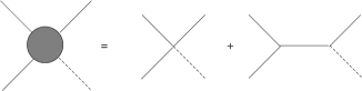
Figure 1: Tree diagrams contributing to the modulation of the three-point function of short wavelength modes (continues lines) in the background of a long wavelength mode (dashed lines).

From the example described above one can also read the information that the four-point correlator in the squeezed limit is not generically written as the products of power spectra, as the universal contribution is. Furthermore, at the linear order in the coupling constant $\lambda$ the four-point correlator in the collapsed limit does not have the form acquired by the universal piece. This happens only at the order ${\cal O}(\lambda^{2})$. Which form is the dominate one depends therefore on the value of the coupling $\lambda$.

4 The four-point correlator in the squeezed limit: alternative methods

In this section we wish to offer two alternative methods to get the non-universal four-point correlator in the squeezed limit. They are based both on the the symmetries of de Sitter and on the OPE technique.

4.1 First method

The fact that the four-point correlator in the squeezed limit may be obtained from the three-point correlator can be also suggested by inspection of the general form (2.27) dictated by the symmetries of de Sitter. Taking the limit of Eq. (3.1), it is easy to see that Eq. (2.27) takes the form

$$\langle\sigma^{I}(\vec{x}_{1})\sigma^{J}(\vec{x}_{2})\sigma^{K}(\vec{x}_{3})\sigma^{L}(\vec{x}_{4})\rangle=\frac{1}{x_{14}^{2w}}\frac{1}{(x_{12}x_{23}x_{13})^{2w/3}}F^{IJKL}\left(\frac{x_{12}}{x_{13}},\frac{x_{23}}{x_{13}}\right)$$ (4.1)

By Fourier transforming the above expression, we get the factorization

$$\langle\sigma^{I}_{\vec{k}_{1}}\sigma^{J}_{\vec{k}_{2}}\sigma^{K}_{\vec{k}_{3}}\sigma^{L}_{\vec{k}_{4}}\rangle^{\prime}\sim P_{\vec{k}_{4}}\widetilde{F}^{IJKL}(k_{14},k_{2},k_{3})=P_{\vec{k}_{4}}\widetilde{F}^{IJKL}(k_{1},k_{2},k_{3}),$$ (4.2)

where in the last equality we have used the fact that $k_{4}\ll k_{1},k_{2},k_{3}$. Then, the function $F^{IJKL}$ depends on just three momenta and conformal invariance specifies this function to be necessarily proportional to the three point function. In particular, in order to calculate the proportionality factor in (4.2) one can make use of the OPEs of the scalar fields. Let us see how this works in a particular model where the light fields mix through a quartic interaction of the type

$$V_{\rm int}\sim\lambda_{IJKL}\sigma^{I}\sigma^{J}\sigma^{K}\sigma^{L}.$$ (4.3)

The OPE for the two fields $\sigma^{I}$ and $\sigma^{J}$ in the (12) channel at the coincident point is

$$\sigma^{I}(\vec{x}_{1})\sigma^{J}(\vec{x}_{2})\!=\!\frac{C_{0}^{IJ}(w)}{x_{12}^{2w}}+\frac{{C^{IJ}}_{M}(w)}{x_{12}^{w}}\sigma^{M}(\vec{x}_{2})+\sigma^{I}(\vec{x}_{2})\sigma^{J}(\vec{x}_{2})+\cdots.$$ (4.4)

Multiplying both sides with $\sigma^{K}(\vec{x}_{3})$ and since $x_{13}\approx 0$, we get

$$\sigma^{I}(\vec{x}_{1})\sigma^{J}(\vec{x}_{2})\sigma^{K}(\vec{x}_{3})=\frac{C_{0}^{IJ}(w)}{x_{12}^{2w}}\sigma^{K}(\vec{x}_{3})+\frac{{C^{IJ}}_{M}(w)}{x_{12}^{w}}\sigma^{M}(\vec{x}_{2})\sigma^{K}(\vec{x}_{3})$$

$$\hskip 99.58464pt+\Big{(}\sigma^{I}(\vec{x}_{2})\sigma^{J}(\vec{x}_{2})\Big{)}\sigma^{K}(\vec{x}_{3})+\cdots.$$ (4.5)

For the operator ${\cal{O}}^{IJ}(\vec{x}_{2})=\sigma^{I}(\vec{x}_{2})\sigma^{J}(\vec{x}_{2})$ we have the OPE

$${\cal{O}}^{IJ}(\vec{x}_{2})\sigma^{K}(\vec{x}_{3})=\frac{D^{IJK}}{x_{23}^{3w}}+\frac{\lambda^{IJKL}}{x_{23}^{2w}}\sigma^{L}(\vec{x}_{3})+\cdots$$ (4.6)

as we assume that the operator ${\cal{O}}^{IJ}\sigma^{K}$ mixes with $\sigma^{L}$ through the quartic interaction. This is due to in field theory is called mixing of composite operators. By using Eqs. (4.4), (4.20) in Eq. (4.5) we then get

$$\sigma^{I}(\vec{x}_{1})\sigma^{J}(\vec{x}_{2})\sigma^{K}(\vec{x}_{3})=\frac{{C^{IJ}}_{M}}{x_{12}^{w}}\frac{C_{0}^{MK}}{x_{12}^{w}x_{23}^{w}}+\frac{D^{IJK}}{x_{23}^{3w}}+\frac{C_{0}^{IJ}(w)}{x_{12}^{2w}}\sigma^{K}(\vec{x}_{3})$$ (4.7)

$$\hskip 99.58464pt+\frac{{C^{IJ}}_{M}}{x_{12}^{w}}\frac{{C^{MK}}_{N}(w)}{x_{23}^{w}}\sigma^{N}(\vec{x}_{3})+\frac{{\lambda^{IJK}}_{N}}{x_{23}^{w}x_{13}^{w}}\sigma^{N}(\vec{x}_{3})\cdots,$$ (4.8)

where for symmetry reasons we have replaced $x_{23}^{2w}$ with $x_{13}^{w}x_{23}^{w}$. Then, it is easy to find that after multiplying the above OPE with $\sigma^{L}(\vec{x}_{4})$, the connected part of the four-point correlator turns out to be

$$\langle\sigma^{I}(\vec{x}_{1})\sigma^{J}(\vec{x}_{2})\sigma^{K}(\vec{x}_{3})\sigma^{L}(\vec{x}_{4})\rangle=\frac{D^{IJKL}}{x_{12}^{w}x_{23}^{w}x_{34}^{2w}}+\rm{permutations},$$ (4.9)

where

$$\framebox{$\displaystyle D^{IJKL}=\lambda^{IJKL}+{C^{IJ}}_{M}C^{MKL}$}.$$ (4.10)

By Fourier transforming the expression (4.10) we may get the four-point function in momentum space

$$\langle\sigma_{\vec{k}_{1}}^{I}\sigma_{\vec{k}_{2}}^{J}\sigma_{\vec{k}_{3}}^{K}\sigma_{\vec{k}_{4}}^{L}\rangle^{\prime}\sim D^{IJKL}C^{-1}_{NPM}\,P_{\vec{k}_{4}}\,\langle\sigma_{\vec{k}_{1}}^{N}\sigma_{\vec{k}_{2}}^{P}\sigma_{\vec{k}_{34}}^{M}\rangle^{\prime}$$

$$\hskip 76.82234pt\sim D^{IJKL}C^{-1}_{NPM}\,P_{\vec{k}_{4}}\,\langle\sigma_{\vec{k}_{1}}^{N}\sigma_{\vec{k}_{2}}^{P}\sigma_{\vec{k}_{3}}^{M}\rangle^{\prime},\,\,\,\,\,\,\,\,\,\,\,\,\,\,\,\,\,\,\,(k_{4}\ll k_{1},k_{2},k_{3}).$$ (4.11)

Therefore, we confirm again that the non-universal contribution to the four-point correlator in the squeezed limit does not have the shape of the universal contribution.

4.2 Second method: Cardy’s trick

For completeness, let us reproduce the expression (3.7) by making use of the conformal symmetries of de Sitter. In order to apply the OPE expansion, we need the operators to be at almost coincident points. In our case, three points are very close and one point is far form the others. So, to make use of the OPE’s, we should bring the remote point $\vec{x}_{4}$ very close to the points $\vec{x}_{1}$,$\vec{x}_{2}$ and $\vec{x}_{3}$. To do this, we use the following trick due to Cardy [26]. We use the fact that under the conformal inversion around an arbitrary point $\vec{x}_{0}$, the conformal inversion (2.15) becomes

$$\vec{x}^{\prime}=\frac{\vec{x}-\vec{x}_{0}}{|\vec{x}-\vec{x}_{0}|^{2}}.$$ (4.12)

In other words, if the point $\vec{x}_{4}$ is very far from the point $\vec{x}_{0}$, then under conformal inversion it becomes very close to it. Under the conformal inversion the four-point correlator transforms as

$$\langle\sigma^{I}(\vec{x}_{1})\sigma^{J}(\vec{x}_{2})\sigma^{K}(\vec{x}_{3})\sigma^{L}(\vec{x}_{4})\rangle=\frac{\langle\sigma^{I}(\vec{x}_{1}^{\prime})\sigma^{J}(\vec{x}_{2}^{\prime})\sigma^{K}(\vec{x}_{3}^{\prime})\sigma^{L}(\vec{x}_{4}^{\prime})\rangle}{|\vec{x}_{1}-\vec{x}_{0}|^{2w}|\vec{x}_{2}-\vec{x}_{0}|^{2w}|\vec{x}_{3}-\vec{x}_{0}|^{2w}|\vec{x}_{4}-\vec{x}_{0}|^{2w}}.$$ (4.13)

In our case, we may do a conformal inversion about the point $\vec{x}_{0}\equiv\vec{x}_{3}$. Then, the point $\vec{x}_{3}$ will remain invariant $(\vec{x}_{3}^{\prime}=\vec{x}_{3})$ and the point $\vec{x}_{4}$ will come close to $\vec{x}_{3}$ as $x^{\prime}_{34}=1/x_{34}\rightarrow 0$. All other distances will be clearly larger that $x^{\prime}_{34}$. Thus, we may use the OPE

$$\sigma^{K}(\vec{x}_{3})\sigma^{L}(\vec{x}^{\prime}_{4})=\frac{\delta^{KL}}{x_{34}^{{}^{\prime}2w}}+\frac{C^{KLM}(g)}{x_{34}^{{}^{\prime}w}}\sigma^{M}(\vec{x}_{3})+\sigma^{K}(\vec{x}_{3})\sigma^{L}(\vec{x}_{3})\cdots,$$ (4.14)

where by $g$ we again denote collectively the couplings. We get therefore from the linear term in the above OPE the connected part

$$\langle\sigma^{I}(\vec{x}_{1}^{\prime})\sigma^{J}(\vec{x}_{2}^{\prime})\sigma^{K}(\vec{x}_{3})\sigma^{L}(\vec{x}_{4}^{\prime})\rangle=\frac{C^{KLM}}{x_{34}^{{}^{\prime}w}}\frac{\langle\sigma^{I}(\vec{x}_{1}^{\prime})\sigma^{J}(\vec{x}_{2}^{\prime})\sigma^{M}(\vec{x}_{3})\rangle}{|\vec{x}_{1}-\vec{x}_{0}|^{2w}|\vec{x}_{2}-\vec{x}_{0}|^{2w}|\vec{x}_{3}-\vec{x}_{0}|^{2w}|\vec{x}_{4}-\vec{x}_{0}|^{2w}}.$$ (4.15)

Now, we go back to the original configuration by doing again a second conformal inversion about the $\vec{x}_{3}$ point. Since the conformal inversion will cancel three terms of the product in Eq. (4.13), we get

$$\langle\sigma^{I}(\vec{x}_{1})\sigma^{J}(\vec{x}_{2})\sigma^{K}(\vec{x}_{3})\sigma^{L}(\vec{x}_{4})\rangle=\frac{C^{KLM}}{x_{34}^{w}}\langle\sigma^{I}(\vec{x}_{1})\sigma^{J}(\vec{x}_{2})\sigma^{M}(\vec{x}_{3})\rangle.$$ (4.16)

By Fourier transforming the above expression we finally obtain the second piece of Eq. (3.7)

$$\langle\sigma^{I}_{\vec{k}_{1}}\sigma^{J}_{\vec{k}_{2}}\sigma^{K}_{\vec{k}_{3}}\sigma^{L}_{\vec{k}_{4}}\rangle^{\prime}\supset{C^{KL}}_{M}P_{\vec{k}_{4}}\langle\sigma^{I}_{\vec{k}_{1}}\sigma^{J}_{\vec{k}_{2}}\sigma^{M}_{\vec{k}_{4}}\rangle^{\prime},\,\,\,\,\,\,(k_{4}\ll k_{1},k_{2},k_{3}).$$ (4.17)

We should stress again that $C^{KLM}$ should be understood in a non-perturbative sense and have a perturbative expansion in the coupling constants $g$, of the form $C^{IJK}(g)=\sum_{n}c^{IJK}_{n}g^{n}$.

In fact, it is easy to generalize the above discussion to the general $n$-point function in the squeezed limit. A simple induction of the above leads to

$$\langle\sigma^{I}_{\vec{k}_{1}}\sigma^{J}_{\vec{k}_{2}}\cdots\sigma^{K}_{\vec{k}_{n-1}}\sigma^{L}_{\vec{k}_{n}}\rangle^{\prime}\supset C^{KLM}P_{\vec{k}_{n}}\langle\sigma^{I}_{\vec{k}_{1}}\sigma^{J}_{\vec{k}_{2}}\cdots\sigma^{M}_{\vec{k}_{n-1}}\rangle^{\prime},\,\,\,\,\,\,(k_{n}\ll k_{1},k_{2},\cdots,k_{n-1}).$$ (4.18)

The first piece of Eq. (3.7) emerges from the quadratic term of the OPE in Eq. (4.14). Indeed, this term gives a contribution of the form

$$\langle\sigma^{I}(\vec{x}_{1}^{\prime})\sigma^{J}(\vec{x}_{2}^{\prime})\sigma^{K}(\vec{x}_{3})\sigma^{L}(\vec{x}_{4}^{\prime})\rangle\supset\frac{\langle\sigma^{I}(\vec{x}_{1}^{\prime})\sigma^{J}(\vec{x}_{2}^{\prime})\sigma^{K}(\vec{x}_{3})\sigma^{L}(\vec{x}_{3})\rangle}{|\vec{x}_{1}-\vec{x}_{0}|^{2w}|\vec{x}_{2}-\vec{x}_{0}|^{2w}|\vec{x}_{3}-\vec{x}_{0}|^{2w}|\vec{x}_{4}-\vec{x}_{0}|^{2w}}.$$ (4.19)

For the operator ${\cal{O}}^{KL}(\vec{x}_{3})=\sigma^{K}(\vec{x}_{3})\sigma^{L}(\vec{x}_{3})$ we have the OPE

$${\cal{O}}^{KL}(\vec{x}_{3})\sigma^{J}(\vec{x}_{2}^{\prime})=\frac{D^{IJK}}{|\vec{x}_{2}^{\prime}-\vec{x}_{3}|^{3w}}+\frac{\lambda^{IJKL}}{|\vec{x}_{2}^{\prime}-\vec{x}_{3}|^{2w}}\sigma^{L}(\vec{x}_{3})+\cdots$$ (4.20)

where we assume again that ${\cal{O}}^{KL}\sigma^{J}$ mixes with $\sigma^{L}$ through the quartic interaction (4.3). Repeating the steps above and after an inverse conformal inversion we get

$$\langle\sigma^{I}(\vec{x}_{1})\sigma^{J}(\vec{x}_{2})\sigma^{K}(\vec{x}_{3})\sigma^{L}(\vec{x}_{4})\rangle\supset\frac{\lambda^{IJKL}}{x_{12}^{w}x_{23}^{w}x_{34}^{2w}}+\rm{permutations},$$ (4.21)

Therefore the total four-point correlator (3.7) may be written after Fourier transforming as in Eq. (4.11) where $D^{IJKL}$ is given by Eq. (4.10).

5 On the non-universal contributions to NG

Having established the form of the non-universal three- and four-point correlator in the squeezed limit, we now focus our attention on their magnitude. We already pointed out that the non-universal contributions can be the dominant ones. For practical purposes, let us consider the squeezed limit of the three-point correlator in a $V(\sigma)=\lambda\sigma^{4}/4!$ model

$$\langle\sigma_{\vec{k}_{1}}\sigma_{\vec{k}_{2}}\sigma_{\vec{k}_{3}}\rangle^{\prime}\simeq-\frac{2}{3}\frac{\lambda\overline{\sigma}}{H^{2}}\,N_{k_{t}}\,P_{\vec{k}_{1}}P_{\vec{k}_{2}},\,\,\,\,\,\,\,\,\,\,\,\,\,\,\,\,\,\,\,\,\,\,\,\,\,\,\,\,\,(k_{1}\ll k_{2}\sim k_{3}).$$ (5.1)

The corresponding contribution to the three-point correlator of the comoving curvature perturbation is

$$\langle\zeta_{\vec{k}_{1}}\zeta_{\vec{k}_{2}}\zeta_{\vec{k}_{3}}\rangle^{\prime}\simeq-\frac{2}{3N^{\prime}}\frac{\lambda\overline{\sigma}}{H^{2}}\,N_{k_{t}}\,P^{\zeta}_{\vec{k}_{1}}P^{\zeta}_{\vec{k}_{2}},\,\,\,\,\,\,\,\,\,\,\,\,\,\,\,\,\,\,\,\,\,\,\,\,\,\,\,\,\,(k_{1}\ll k_{2}\sim k_{3})$$ (5.2)

leading to a non-universal contribution to the nonlinear parameter $f_{\rm NL}$ given by

$$f_{\rm NL}^{\rm n-un}\simeq-\frac{5}{18N^{\prime}}\frac{\lambda\overline{\sigma}}{H^{2}}N_{k_{t}}=-\frac{5}{36\pi}\frac{\lambda\overline{\sigma}}{H}\frac{N_{k_{t}}}{{\cal P}_{\zeta}^{1/2}}\simeq-\frac{5\sqrt{2\lambda}}{36\pi}\frac{m(\overline{\sigma})}{H}\frac{N_{k_{t}}}{{\cal P}_{\zeta}^{1/2}}\simeq-65\left(\frac{\lambda}{10^{-2}}\right)^{1/2}\left(\frac{m(\overline{\sigma})/H}{10^{-2}}\right)\left(\frac{N_{k_{t}}}{50}\right),$$

where we have defined the quantity ${\cal P}_{\zeta}=(k^{3}/2\pi^{2})P^{\zeta}_{\vec{k}}=N^{\prime 2}(H/2\pi)^{2}\simeq 2.3\cdot 10^{-9}$ and the (field dependent) Higgs mass $m(\overline{\sigma})^{2}=\lambda\overline{\sigma}^{2}/2$. Analogously we find

$$g_{\rm NL}^{\rm n-un}\simeq-\frac{25}{54\cdot 3N^{\prime 2}}\frac{\lambda}{H^{2}}N_{k_{t}}=-\frac{25\lambda}{54\cdot 3(2\pi)^{2}}\frac{N_{k_{t}}}{{\cal P}_{\zeta}}\simeq-10^{6}\left(\frac{\lambda}{10^{-2}}\right)\left(\frac{N_{k_{t}}}{50}\right).$$ (5.4)

We see that the nonlinearities generated by the non-universal pieces can be substantial, confirming previous findings [18, 17, 19, 20]. Furthermore, we also deduce that it is quite simple to have models in which $g_{\rm NL}\,\raisebox{-1.1625pt}{${}_{\textstyle>}\atop{}^{\textstyle\sim}$}\,f_{\rm NL}^{2}$ (in absolute values), a simple $\lambda\sigma^{4}$ model will do it as long as $H/\overline{\sigma}\,\raisebox{-1.1625pt}{${}_{\textstyle>}\atop{}^{\textstyle\sim}$}\,\sqrt{\lambda}$.

6 Conclusions

In this paper we have made use of the OPE technique and, partly, of the symmetries of the de Sitter epoch, to characterize the NG four-point correlator of the curvature perturbation in multifield inflation. In particular we have pointed out that

• The contribution to the squeezed limit of the four-point correlator coming from the intrinsic NG of the light fields at horizon crossing (which we dubbed non-universal) can be larger than the superhorizon contributions (we dubbed them universal) generated even if the light fields are gaussian.

• The shape of the non-universal contribution to the squeezed limit of the four-point correlator can be expressed in terms of the three-point correlator. Nevertheless, in general the shapes of the universal and non-universal contributions are different as the three-point correlator is note evaluated in the squeezed limit.

Therefore, particular care needs to be taken when studying the effects of the primordial NG on real observables, e.g. the scale dependence of the local halo bias in the presence of NG, as the squeezed limit of the four-point correlator is not expressible in terms of products of power spectra. The consequences of our findings will be investigated elsewhere.

References

• [1] N. Bartolo, E. Komatsu, S. Matarrese and A. Riotto, Phys. Rept.  402, 103 (2004).
• [2] D. H. Lyth and A. Riotto, Phys. Rept. 314 1 (1999); A. Riotto, hep-ph/0210162.
• [3] K. Enqvist and M. S. Sloth, Nucl. Phys. B 626, 395 (2002).
• [4] D. H. Lyth and D. Wands, Phys. Lett. B 524, 5 (2002).
• [5] T. Moroi and T. Takahashi, Phys. Lett. B 522, 215 (2001) [Erratum-ibid. B 539, 303 (2002)].
• [6] G. Dvali, A. Gruzinov and M. Zaldarriaga, Phys. Rev. D 69, 023505 (2004); L. Kofman; G. Dvali, A. Gruzinov and M. Zaldarriaga, Phys. Rev. D 69, 083505 (2004).
• [7] D. H. Lyth, JCAP 0511, 006 (2005); D. H. Lyth and A. Riotto, Phys. Rev. Lett.  97, 121301 (2006).
• [8] E. W. Kolb, A. Riotto and A. Vallinotto, Phys. Rev. D 71, 043513 (2005).
• [9] N. Dalal, O. Dore, D. Huterer and A. Shirokov, Phys. Rev. D 77, 123514 (2008).
• [10] V. Acquaviva, N. Bartolo, S. Matarrese and A. Riotto, Nucl. Phys. B 667, 119 (2003).
• [11] J. Maldacena, JHEP 0305, 013 (2003).
• [12] A. Kehagias and A. Riotto, Nucl. Phys. B 864, 492 (2012).
• [13] P. Creminelli, J. Norena and M. Simonovic, arXiv:1203.4595 [hep-th]; K. Hinterbichler, L. Hui and J. Khoury, arXiv:1203.6351.
• [14] M. Sasaki and E. D. Stewart, Prog. Theor. Phys.  95, 71 (1996).
• [15] E. Komatsu et al. [WMAP Collaboration], Astrophys. J. Suppl.  192, 18 (2011).
• [16] J. Smidt, A. Amblard, A. Cooray, A. Heavens, D. Munshi and P. Serra, arXiv:1001.5026 [astro-ph.CO].
• [17] N. Bartolo, S. Matarrese and A. Riotto, Phys. Rev. D 64, 123504 (2001).
• [18] M. Zaldarriaga, Phys. Rev. D 69, 043508 (2004).
• [19] F. Bernardeau and J. -P. Uzan, Phys. Rev. D 67, 121301 (2003).
• [20] F. Bernardeau and J. -P. Uzan, Phys. Rev. D 70, 043533 (2004).
• [21] I. Antoniadis, P. O. Mazur and E. Mottola, “Conformal Invariance, Dark Energy, and CMB Non-Gaussianity,” arXiv:1103.4164 [gr-qc].
• [22] P. Creminelli, “Conformal invariance of scalar perturbations in inflation,” Phys. Rev. D 85, 041302 (2012).
• [23] K. G. Wilson, Phys. Rev.  179, 1499 (1969).
• [24] K. G. Wilson, Phys. Rev. B 4, 3174 (1971); ibidem Phys. Rev. B 4, 3184 (1971).
• [25] W. Zimmermann, ”Local operator products and renormalization in quantum field theory” in : “Lectures on Elementary Particles and Quantum Field Theory”, Brandeis Summer Institute 1970, S. Deser, M. Grisaru, H. Pendleton eds. MIT Press 1970, Cambridge Ma.
• [26] J.L. Cardy, Nucl. Phys. B290, 355 (1987).