Stochastic Particle Acceleration and the Problem of Background Plasma Overheating

Abstract

The origin of hard X-ray (HXR) excess emission from clusters of galaxies is still an enigma, whose nature is debated. One of the possible mechanism to produce this emission is the bremsstrahlung model. However, previous analytical and numerical calculations showed that in this case the intracluster plasma had to be overheated very fast because suprathermal electrons emitting the HXR excess lose their energy mainly by Coulomb losses, i.e., they heat the background plasma. It was concluded also from these investigations that it is problematic to produce emitting electrons from a background plasma by stochastic (Fermi) acceleration because the energy supplied by external sources in the form of Fermi acceleration is quickly absorbed by the background plasma. In other words the Fermi acceleration is ineffective for particle acceleration. We revisited this problem and found that at some parameter of acceleration the rate of plasma heating is rather low and the acceleration tails of non-thermal particles can be generated and exist for a long time while the plasma temperature is almost constant. We showed also that for some regime of acceleration the plasma cools down instead of being heated up, even though external sources (in the form of external acceleration) supply energy to the system. The reason is that the acceleration withdraws effectively high energy particles from the thermal pool (analogue of Maxwell demon).

1 Introduction

One of the most important problem in astrophysics is the problem of particle acceleration. The general expression for acceleration of a charged particle is

$$\frac{d}{dt}(\gamma m{\bf v})=Ze\left({\bf E}+\frac{1}{c}{\bf v}\times{\bf B}\right)\,,$$ (1)

where ${\bf E}$ and ${\bf B}$ are the electric and magnetic field strength, ${\bf v}$ is the velocity of particle and $\gamma=1/\sqrt{1-v^{2}/c^{2}}$. In most astrophysical conditions static electrical fields cannot be maintained because of a very high electrical conductivity. Therefore the acceleration can be associated either with non-stationary electric fields (electromagnetic waves) or with time-varying magnetic fields. In the latter case the work can be done by the induced electric field

$$\frac{1}{c}\frac{\partial{\bf B}}{\partial t}=-{\bf\nabla\times E}\,.$$ (2)

The basic idea of acceleration by electromagnetic inhomogeneities in astrophysical conditions was suggested by Fermi (1949, 1954) who assumed that the Galactic cosmic rays (CRs) were accelerated by collisions of charged particles with fluctuations of magnetic fields (magnetic clouds) moving chaotically with the velocity dispersion $u$. One of the features of this theory was that it yielded naturally a power-law spectrum of accelerated particles. The rate of particle acceleration by this stochastic mechanism is about

$$\left(\frac{d\mathcal{E}}{dt}\right)_{F}\sim\frac{u^{2}}{v^{2}\tau}\mathcal{E}\,,$$ (3)

where $\mathcal{E}$ and $v$ are the particle kinetic energy and velocity, and $\tau$ is the average time of particle collision with the clouds. This rate of acceleration is slow because $u\ll v$. In kinetic equations, the Fermi (stochastic) acceleration is described as momentum diffusion (see e.g., Toptygin, 1985)

$$\frac{\partial f}{\partial t}-\frac{1}{p^{2}}\frac{\partial}{\partial p}\left[D_{F}(p)p^{2}\frac{\partial f}{\partial p}\right]+\hat{L}f=0\,,$$ (4)

with the diffusion coefficient $D_{F}(p)$ in the form

$$D_{F}(p)\sim p^{2}\frac{u^{2}}{v^{2}\tau}\,.$$ (5)

Here $f(p,t)$ is the particle distribution function, $p$ is the particle momentum, $t$ is the time, and the operator $\hat{L}$ describes particle spatial propagation and their momentum losses.

In spite of its low efficiency, stochastic acceleration may be essential for particle acceleration in solar flares (see e.g., Miller et al., 1990; Petrosian, 2012), in the interstellar medium of the Galaxy (Berezinskii et al., 1990) and near the Galactic center (see e.g., Mertsch & Sarkar, 2011).

The problem of stochastic particle acceleration in galaxy clusters arose from observations in the hard X-ray (HXR) energy range (see e.g., Fusco-Femiano et al., 1999, 2007; Rephaeli et al., 1999, 2008; Eckert et al., 2008; Nevalainen, 2009; Ajello et al., 2010) which showed an emission excess above the equilibrium thermal X-ray spectrum.

One of the several interpretations of the HXR excess from the Coma cluster in the range 20-80 keV was an assumption that it was produced by bremsstrahlung radiation of suprathermal electrons (see e.g., Enßlin et al., 1999) accelerated in the intracluster medium. However, this model was criticized by Petrosian (2001) who concluded from simple estimates that in this case the intracluster plasma in Coma had to be overheated very fast. The point is that suprathermal electrons emitting the HXR excess lose their energy mainly by Coulomb losses, i.e., they lose their energy by heating the background plasma. If these electrons generate an X-ray flux $L_{X}$ by bremsstrahlung, they transfer the energy flux $L_{C}$ to the background plasma. The necessary energy input is estimated as

$$L_{C}\sim L_{X}\left[\frac{(d\mathcal{E}/dt)_{C}}{(d\mathcal{E}/dt)_{BR}}\right]\,,$$ (6)

where $(d\mathcal{E}/dt)_{C}$ and $(d\mathcal{E}/dt)_{BR}$ are the rates of Coulomb and bremsstrahlung losses, respectively. In the keV energy range $(d\mathcal{E}/dt)_{C}\gg(d\mathcal{E}/dt)_{BR}$, and this seems to make plasma overheating inevitable. However, we should point out that in effect particle acceleration may also be accompanied by plasma cooling due to run-away flux of high energy particles from thermal pool, and more careful analysis is necessary to define which of these effects (plasma heating or cooling) prevails. This analysis is presented in the following sections.

2 Review of Particle Acceleration from Background Plasma

A natural source for suprathermal particles is stochastic acceleration of seed particles from a background plasma. These particles are accelerated when the rate of acceleration $(d\mathcal{E}/dt)_{F}$ exceeds the rate of the Coulomb losses $(d\mathcal{E}/dt)_{C}$. A characteristic energy called the injection energy $\mathcal{E}_{\rm inj}$ is the energy above which a non-thermal spectrum is formed by acceleration. It is determined by equating these rates of acceleration and loss.

The kinetic equation in the particle momentum space describing stochastic particle acceleration from background plasma has the form (assume isotropic distribution)

$${{\partial f}\over{\partial t}}+{1\over p^{2}}{\partial\over{\partial p}}p^{2}\left[\left(\frac{dp}{dt}\right)_{C}f-\left\{D_{C}(p)+D_{F}(p)\right\}{{\partial f}\over{\partial p}}\right]=0\,,$$ (7)

where $D_{F}(p)$ is the diffusion coefficient of stochastic (Fermi) acceleration, and $(dp/dt)_{C}$ and $D_{C}(p)$ describe particle momentum losses and diffusion due to Coulomb collisions. These coefficients are calculated from the total distribution function $f$ (see Appendix A), and therefore in general the equation is nonlinear.

2.1 Linear Approximation

An analytical solution of this equation for the case of weak acceleration from a background plasma with temperature $T$ was obtained by Gurevich (1960). The term of stochastic acceleration was taken in the phenomenological form

$$D_{F}(p)=\alpha p^{2}\,.$$ (8)

The analysis was provided for the case when the characteristic time of stochastic acceleration,

$$\tau_{F}=p^{2}/D_{F}\,,$$ (9)

is much larger than the time of thermal particle collisions, $\tau_{th}$,

$$\tau_{th}\simeq\sqrt{\frac{2}{m}}~{}\frac{m_{e}(k_{\rm B}T)^{3/2}}{\pi Ne^{4}\ln\Lambda}\,,$$ (10)

where $N$ is the density and $T$ is the temperature of background plasma, $\ln\Lambda$ is the Coulomb logarithm, $m_{e}$ is the electron rest mass and $m$ is the mass of accelerated particles.

In this case the injection energy $\mathcal{E}_{\rm inj}$ is much larger than the plasma temperature, $\mathcal{E}_{\rm inj}\gg k_{\rm B}T$. Coulomb collisions keep the equilibrium Maxwellian distribution for most part of the momentum range, and the coefficients of Eq. (7) for nonrelativistic momenta $p\gg\sqrt{2mk_{\rm B}T}$ (as used by Gurevich, 1960) for the Maxwellian distribution function. For $\tau_{th}\ll\tau_{F}$, significant distortions from the equilibrium Maxwellian state are expected only for very large values of momenta and a very small fraction of thermal particles is accelerated. Therefore Gurevich (1960) assumed that the number of particles $N(t)$ in the momentum range $p<p_{\rm inj}$ varies very slowly with time $t$, $N(t)=N_{0}-St$, where $N_{0}$ is the initial particle density and a small run-away flux $S$ is generated at relatively high momentum range. The run-away flux for the case of slow acceleration can be described as

$$S(p)=S_{0}{4\over\sqrt{\pi}}\int\limits^{{\bar{p}}}_{0}x^{2}e^{-x^{2}}dx=S_{0}\left[{\rm erf}\left({\bar{p}}\right)-{2\over\sqrt{\pi}}\,{\bar{p}}\,e^{-{\bar{p}}^{2}}\right]\,,$$ (11)

where ${\rm erf}(z)$ is the error function, ${\bar{p}}=p/\sqrt{2mk_{\rm B}T}$, and the constant $S_{0}$ is derived from boundary conditions. The flux is zero at $p=0$ but when $p\gg\sqrt{2mk_{\rm B}T}$, it reaches a maximum value $S(p)=S_{0}$ as shown in Fig. 1.

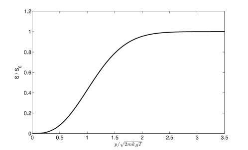
Figure 1: Run-away flux $S$ as a function of the dimensionless momentum $p/\sqrt{2mk_{\rm B}T}$.

In the momentum range where $S(p)\simeq S_{0}$ the distribution function is non-Maxwellian and it is described by the kinetic equation

$$p^{2}\left[\left(\frac{dp}{dt}\right)_{C}f-\left\{D_{C}(p)+D_{F}(p)\right\}{{\partial f}\over{\partial p}}\right]=S_{0}\,.$$ (12)

The acceleration forms a nonthermal component of the spectrum in the range $p>p_{\rm inj}$ where $p_{\rm inj}$ is the solution of equation

$$p_{\rm inj}={D_{F}(p_{\rm inj})\over(dp/dt)_{C}}\,.$$ (13)

However, if $D_{F}(p)\neq 0$ in the range $p<p_{\rm inj}$, a solution of this equation describes also an excess of the distribution function above the equilibrium Maxwellian distribution in momentum ranges both above and below $p_{\rm inj}$ (see Gurevich, 1960). This excess at $p<p_{\rm inj}$ is formed by Coulomb collisions in the transition range between the thermal (Maxwellian) and non-thermal parts of the spectrum. If the HXR excess is due to bremsstrahlung emission of electrons from this transition region then the relation (6) used by Petrosian (2001) cannot be applied to the estimate of $L_{C}$ and more accurate calculations are necessary.

Bremsstrahlung emission of electrons from the transition region was calculated in Dogiel (2000); Liang et al. (2002); Dogiel et al. (2007). The conclusion is that the necessary energy input $L_{C}$ for Coma was about one order of magnitude less than obtained by Petrosian (2001). This may solve the problem of the plasma overheating. However, their linear analysis of equation (7) does not include variations of temperature $T$ which is supposed to be constant.

2.2 Non-Linear Treatment

More reliable conclusions can be derived from analyses of the nonlinear equation in the form similar to those used by MacDonald et al. (1957), when a feedback of accelerated particles on the plasma temperature is taken into account. Very recently Wolfe & Melia (2006) and Petrosian & East (2008) provided similar numerical analysis for the case of stochastic acceleration from a background plasma.

The nonlinear kinetic equation describing particle Coulomb collisions is derived in Landau & Lifshitz (1981) (see Appendix A). Using this theory Nayakshin & Melia (1998) derived coefficients of this equation for the case of isotropic and homogeneous distribution function for non-relativistic and ultra-relativistic particles. Later, Wolfe & Melia (2006) extended their analysis to the general case of anisotropic distribution function.

Numerical analysis of these equations has been performed by Wolfe & Melia (2006) for the isotropic stochastic acceleration in the form

$$D_{F}(p)=\alpha p^{\varsigma}\theta(p-1/2)\,.$$ (14)

Wolfe & Melia (2006) stated that the continuous stochastic acceleration of thermal electrons produced a nonthermal tail. But for the hard X-ray emission in the Coma Cluster this model actually cannot work because the energy gained by the particles is distributed to the whole plasma on a timescale much shorter than that of the acceleration process itself. Moreover, bremsstrahlung is relatively inefficient to cool the accelerated electrons, the energy of this tail is quickly dumped into the thermal background plasma and heat the plasma.

Similarly, Petrosian & East (2008) obtained numerical solutions of the nonlinear isotropic kinetic equations which included effects of plasma heating for the stochastic diffusion in the form

$$D_{F}(\mathcal{E})=\frac{\mathcal{E}^{2}}{\zeta(\mathcal{E})\tau_{0}(1+\mathcal{E}_{c}/\mathcal{E})^{q}}\,,$$ (15)

where $\mathcal{E}=\sqrt{p^{2}+1}-1$ is the kinetic energy normalized to $mc^{2}$, $\zeta(\mathcal{E})=(2-\gamma^{-2})/(1+\gamma^{-1})$, and $\tau_{0}$, $\mathcal{E}_{c}$ and $q$ are free parameters.

Petrosian & East (2008) concluded that their calculations confirmed qualitatively results of Dogiel et al. (2007) that the required input energy $L_{C}$ was lower than that follows from the estimate (6) but by a factor of 2 or 3 only, and that did not solve the problem of plasma overheating. Besides, they argued that their calculations confirmed results of Wolfe & Melia (2006) that stochastic acceleration could not work in clusters because the energy gained by the particles was distributed to the whole plasma on timescales much shorter than that of the acceleration process. At acceleration rates smaller than the thermalization rate of the background plasma, there is very little acceleration. The primary effect of acceleration is heating of the plasma. In the opposite case, at higher energizing rates, a distinguishable nonthermal tail is developed, but this is again accompanied by an unacceptably high rate of heating.

In other words it follows from these investigations that it is problematic to accelerate particles from a background plasma because the main effect of this acceleration is plasma overheating. The energy supplied by external sources in the form of stochastic (Fermi) acceleration is quickly absorbed by a background plasma. An interesting question arises: whether any conditions exist when the stochastic acceleration generate prominent nonthermal tails while the plasma is not overheated and its temperature varies relatively slowly. From the analysis in the following sections, we argue that the answer is affirmative.

3 Particle Acceleration from Background Plasma: Quasi-Linear Approximation

First, we estimate variations of plasma temperature derived in quasi-stationary approximations when the distribution function can be presented as $f=f(p,N,T)$. In this case,

$$\frac{\partial f}{\partial t}=\frac{\partial f}{\partial N}\frac{dN}{dt}+\frac{\partial f}{\partial T}\frac{dT}{dt}\,.$$ (16)

where $N=N(t)$ and $T=T(t)$ are slowly varying functions of $t$.

3.1 Distribution function

In this subsection we investigate the isotropic form of the kinetic equation (A1). This equation describes stochastic particle acceleration from background plasma and it is exactly the same as Eq. (7). The appropriate boundary conditions are Eqs. (A5) & (A6). Recall that the particle momentum has been normalized to $mc$. Here and in the following the temperature $T$ is indeed the thermal energy $k_{\rm B}T$ normalized to $mc^{2}$. The particle kinetic energy $\mathcal{E}=\sqrt{p^{2}+1}-1$ is also normalized to $mc^{2}$. The coefficients $(dp/dt)_{C}(p)$, $D_{C}(p)$ and $D_{F}(p)$ are normalized accordingly.

The stochastic Fermi acceleration is supposed to be isotropic and has a phenomenological form as

$$D_{F}(p)=\alpha p^{\varsigma}\theta(p-p_{0})\,,$$ (17)

where $\alpha$, $\varsigma$ and $p_{0}$ are arbitrary parameters. The problem is characterized also by the injection momentum

$$\alpha p_{\rm inj}^{\varsigma}=-p_{\rm inj}\left.\left({dp\over dt}\right)_{c}\right|_{p=p_{\rm inj}}\,.$$ (18)

The acceleration is effective in the momentum range $p>{\rm max}\{p_{0},p_{\rm inj}\}$.

Similar to Gurevich (1960) we assume that the acceleration time $\tau_{F}$, is much longer than the time of thermal particle collisions $\tau_{th}$, i.e., values of $p_{\rm inj}$ or $p_{0}$ are large and one of the corresponding energy values is much higher than the temperature,

$$T\ll{\rm max}(\mathcal{E}_{\rm inj},\mathcal{E}_{0})\,.$$ (19)

In this case, Coulomb collisions keep the equilibrium Maxwellian distribution over an extended momentum range with a significant deviation from this distribution at very large momenta, i.e., a small part of thermal particles is accelerated. The number of non-thermal particles generated by the acceleration $N_{n}$ in this case is much smaller than the number of thermal particles $N$, $N_{n}/N\ll 1$.

Below we present the distribution function and the coefficients of the kinetic equation as series expansions over the small parameter $\epsilon=N_{n}/N\ll 1$,

$$f(p,t) =f_{0}(p,t)+f_{1}(p,t)+O\left(\epsilon^{2}\right)\,,$$

$$D_{c}(p,t) =D_{0}(p,t)+D_{1}(p,t)+O\left(\epsilon^{2}\right)\,,$$ (20)

$$\left({dp\over dt}\right)_{c}(p,t) =\left({dp\over dt}\right)_{0}(p,t)+\left({dp\over dt}\right)_{1}(p,t)+O\left(\epsilon^{2}\right)\,.$$

Here $O\left(\epsilon^{i}\right)$ denotes terms of order $\epsilon^{i}$ or above. Note that $f_{i}(p,t)=O(\epsilon^{i})$, $D_{0}$ and $(dp/dt)_{0}$ are calculated from Eq. (A2) for the function $f_{0}$, and $D_{1}$ and $(dp/dt)_{1}$ for the function $f_{1}$, etc.

In the quasi-stationary approximation the derivative $\partial f/\partial t$ can be presented in the form (16). The derivatives $dN/dt$ and $dT/dt$ can be presented as series $dN/dt=O(\epsilon)$ and $dT/dt=O(\epsilon)$, because without acceleration ($N_{n}=0$) we have $dN/dt=0$ and $dT/dt=0$. Here we have

$$\frac{\partial f}{\partial t}=\frac{\partial f_{0}}{\partial t}+O\left(\epsilon^{2}\right)\,,$$ (21)

and ${\partial f_{0}}/{\partial t}$ is of the order of $\epsilon$.

It is convenient to express the distribution function as

$$f(p)=f^{I}(p)\theta(p_{0}-p)+f^{II}(p)\theta(p-p_{0})\,.$$ (22)

First, we find the solution of Eq. (7) in the momentum range $0<p<p_{0}$ where the acceleration term vanishes and $f=f^{I}$ (see Eq. (22)). In zero order of expansion (no acceleration) the function $f_{0}$ is Maxwellian

$$f^{I}_{0}(p)=C_{0}\exp\left[\int_{0}^{p}\left({dp\over dt}\right)_{0}{dp\over D_{0}}\right]=C_{0}\exp(-\mathcal{E}/T)\,,$$ (23)

where $D_{0}$ and $(dp/dt)_{0}$ are the Maxwellian kinetic coefficients. For $p\gg\sqrt{T^{2}+1}-1$ the Bethe-Bloch approximation for the these coefficients is

$$\left({dp\over dt}\right)_{0} =-A\left(1+{1\over p^{2}}\right)\,,$$ (24)

$$D_{0} =-T\sqrt{1+{1\over p^{2}}}\left({dp\over dt}\right)_{0}=AT\left(1+{1\over p^{2}}\right)^{3/2}\,.$$

Here and below

$$A=4\pi r_{e}^{2}cN\ln\Lambda\,.$$ (25)

The characteristic time of Coulomb losses for a particle with momentum $p$ (in unit of $mc$) is

$$\tau_{C}(p)\sim\frac{p^{3}}{A(p^{2}+1)}\,.$$ (26)

Constant $C_{0}$ is estimated from the normalization condition

$$C_{0}=N\left[\int\limits_{0}^{p_{0}}p^{2}f^{I}_{0}(p)dp\right]^{-1}\approx\frac{N\exp(-T^{-1})}{TK_{2}(T^{-1})}\,,$$ (27)

where $K_{2}(x)$ is the modified Bessel function. For non-relativistic temperatures ($T\ll 1$) we obtain

$$C_{0}\approx N\sqrt{\frac{2}{\pi}}T^{-3/2}\,.$$ (28)

The kinetic equation for the function $f^{I}_{1}$ can be rewritten as

$$\frac{1}{p^{2}}\frac{\partial}{\partial p}p^{2}\left[D_{0}(p)\frac{\partial f^{I}_{1}}{\partial p}+D_{1}(p)\frac{\partial f^{I}_{0}}{\partial p}-\left(\frac{dp}{dt}\right)_{0}f^{I}_{1}-\left(\frac{dp}{dt}\right)_{1}f^{I}_{0}\right]=\frac{\partial f^{I}_{0}}{\partial t}+O\left(\epsilon^{2}\right)\,.$$ (29)

Integrating the above equation from 0 to $p$ gives

$$p^{2}\left[D_{0}(p)\frac{\partial f^{I}_{1}}{\partial p}-\left(\frac{dp}{dt}\right)_{0}f^{I}_{1}\right]=-S=-\left(S_{1}+S_{2}\right)\,,$$ (30)

where $S$ is the flux of particles through the point $p$. Here

$$S_{1}=-\frac{dN(p,t)}{dt}=-\frac{\partial}{\partial t}\int\limits_{0}^{p}u^{2}f^{I}_{0}(u)du\,,$$ (31)

$$S_{2}=p^{2}\left[D_{1}(p)\frac{\partial f^{I}_{0}}{\partial p}-\left({dp\over dt}\right)_{1}f^{I}_{0}(p)\right]\,.$$ (32)

The flux $S_{1}$ describes a particle leakage (in momentum space) caused by the acceleration. It generates a slow decrease of particle number in the thermal region. The flux $S_{2}$ causes the plasma heating and temperature variations with time.

Thus, the solution of Eq. (30) is

$$f^{I}_{1}(p)=\exp(-\mathcal{E}/T)\left[C_{1}-\int\limits_{0}^{p}\frac{S(u)}{u^{2}D_{0}(u)}\exp(\mathcal{E}/T)du\right]\,.$$ (33)

As in Gurevich (1960) the value of the constant $C_{1}$ can be derived from the normalization condition

$$\int\limits_{0}^{p_{0}}p^{2}f^{I}_{1}(p)dp=0\,.$$ (34)

The kinetic coefficients $D_{1}$ and $(dp/dt)_{1}$ are calculated for the function $f^{I}_{1}+f^{II}$. Therefore Eq. (33) is an integral equation for $f^{I}_{1}(p)$ which should be added by an equation for $f^{II}(p)$. The asymptotic form of $f^{I}_{1}(p)$ for large values of $p$ can easily be derived. Indeed, if $\mathcal{E}\gg T$ then $S_{1}(p)=O(\epsilon)$ while $S_{2}(p)\sim O(\epsilon)\exp(-\mathcal{E}/T)\ll S_{1}$. Therefore $S_{2}(p)$ can be neglected. As one can see from Eq. (31) the flux $S_{1}(p)$ remains almost constant for sufficiently large $p$ (see Fig. 1). So with a high degree of accuracy we can put $S_{1}(p)=S_{N}\equiv-dN/dt$, which is the same as $S_{0}$ in Gurevich (1960).

It follows from Eqs. (33) and (34) that the constant $C_{1}$ is

$$C_{1}\approx S_{N}\tau_{C}(p_{0})\sqrt{\frac{2}{\pi}}T^{-3/2}\,,$$ (35)

where $\tau_{C}(p_{0})$ is the characteristic time of Coulomb collision for the particle momentum $p=p_{0}$ (for $\tau_{F}$ and $\tau_{C}$ see Eqs. (9) and (26)). Thus, for the estimation of $S_{N}$ obtained in subsection 3.3 we have

$$C_{1}\sim{N\over T^{3/2}}\exp\left(-\frac{\mathcal{E}_{0}}{T}\right)\frac{\tau_{C}(p_{0})}{\tau_{F}(p_{0})}\sim{N\over T^{3/2}}\exp\left(-\frac{\mathcal{E}_{0}}{T}\right)\ll C_{0}\,.$$ (36)

The distribution function in the range $p<p_{0}$ can be written as

$$f^{I}(p)\simeq f^{I}_{0}(p)+f^{I}_{1}(p)$$

$$\quad\quad=\frac{N}{TK_{2}(T^{-1})}\exp\left(-\frac{\xi}{T}\right)-\frac{S_{N}}{AT}\left[\frac{1}{T}\exp\left(-\frac{\xi}{T}\right)Ei\left(\frac{\xi}{T}\right)-\frac{1}{\xi}\right]\,,$$ (37)

where $\xi=\sqrt{p^{2}+1}=\mathcal{E}+1$ is the total energy of particle and

$$Ei(z)=\int\limits_{-\infty}^{z}\frac{\exp(x)}{x}dx\,.$$ (38)

For non-relativistic temperatures $\xi/T\gg 1$ the expansion of $Ei(z)$ for $z\gg 1$ is

$$Ei(z)=\frac{\exp(z)}{z}\sum\limits_{k=0}^{\infty}\frac{k!}{z^{k}}\,.$$ (39)

Thus for large values of $p$

$$f^{I}(p)=\sqrt{\frac{2}{\pi}}\frac{N}{T^{3/2}}\exp\left(-\frac{\mathcal{E}}{T}\right)-\frac{S_{N}}{A(p^{2}+1)}\,.$$ (40)

The distributions function Eq. (3.1) can be presented in the form

$$f^{I}(p)=\left\{\begin{array}[]{l}f_{0}^{I}(p)+O(\epsilon)\,,\mbox{ for }\mathcal{E}\leq T\\ f_{0}^{I}(p)-\frac{S_{N}}{A(p^{2}+1)}+O\left(\epsilon^{2}\right)\,,\mbox{ for }\mathcal{E}_{0}\geq\mathcal{E}\gg T\end{array}\right.$$ (41)

In the range $p\geq p_{0}$ the acceleration cannot be neglected. With the constant flux $S_{N}$ of particles the equation for the distribution function $f^{II}$ in this region reads

$$p^{2}\left[\left\{D_{0}(p)+D_{F}(p)\right\}\frac{\partial f^{II}}{\partial p}-\left(\frac{dp}{dt}\right)_{0}f^{II}\right]=-S_{N}\,.$$ (42)

The general solution of this equation is (see, e.g., Gurevich, 1960)

$$f^{II}(p)=C^{II}\exp\left\{\int\limits_{0}^{p}\frac{(dp/dt)_{0}(u)du}{D_{F}(u)+D_{0}(u)}\right\}$$

$$-S_{N}\exp\left\{\int\limits_{0}^{p}\frac{(dp/dt)_{0}(u)du}{D_{F}(u)+D_{0}(u)}\right\}\int\limits_{0}^{p}\frac{v^{-2}dv}{D_{F}(v)+D_{0}(v)}\exp\left\{-\int\limits_{0}^{v}\frac{(dp/dt)_{0}(u)du}{D_{F}(u)+D_{0}(u)}\right\}\,.$$ (43)

The constant $C^{II}$ can be estimated from the continuity condition at $p=p_{0}$: $f^{I}(p_{0})=f^{II}(p_{0})$ while the value of $S_{N}$ can be estimated from the second boundary condition: $f^{II}(p_{\rm max})=0$.

For $p\gg p_{\rm inj}$, we can assume acceleration dominates Coulomb loss. It is easy to show from Eq. (42) and Eq. (17) that the function $f^{II}(p)$ is a power-law

$$f^{II}(p)=\tilde{C}_{1}+\frac{S_{N}}{\alpha(\varsigma+1)}p^{-\varsigma-1}\,,$$ (44)

where $\tilde{C}_{1}$ is a constant.

3.2 Plasma heating rate

Using the total distribution function $f$ (see Eq. (22), where $f^{I}$ and $f^{II}$ are determined by Eqs. (41) & (3.1)), we can calculate the kinetic coefficients (A2) for the nonlinear equation (7), and then estimate the temperature variations of the background plasma caused by particle acceleration. In this case the stochastic Fermi momentum diffusion describes the energy supply into the system by external sources. Generally speaking, energy supply can vary with time, but usually it is assumed that external sources keep a stationary level of acceleration such that $D_{F}$ is constant.

The total energy input into the system is

$$\dot{W}_{\rm ext}=-\int\limits_{0}^{\infty}\mathcal{E}\frac{\partial}{\partial p}\left[p^{2}D_{F}\frac{\partial f}{\partial p}\right]\,dp\,.$$ (45)

It is a function of time even if $D_{F}$ is constant, because the distributions function $f$ is time dependent.

Note that Coulomb collisions do not change the total energy in the system, therefore we have

$$\int\limits_{0}^{\infty}\mathcal{E}\frac{\partial}{\partial p}p^{2}\left[\left(\frac{dp}{dt}\right)_{C}f-D_{C}(p){{\partial f}\over{\partial p}}\right]\,dp=0\,.$$ (46)

This condition is valid for any function $f$ if the kinetic coefficients $(dp/dt)_{C}$ and $D_{C}(p)$ are calculated from Eq. (A2) for this function $f$.

The energy supplied by the stochastic Fermi acceleration is distributed over the spectrum in the form of accelerated particles and a heated plasma, because accelerated particles lose their energy by Coulomb collisions and thus transfer a part of their energy to thermal particles. Variations of $dT/dt$ in the quasi-equilibrium part of the spectrum can be derived from estimates of the energy flux into the region $p<p_{0}$ which is

$$\dot{W_{0}}=\frac{\partial}{\partial t}\int\limits_{0}^{p_{0}}p^{2}\mathcal{E}f^{I}(p)dp=\int\limits_{0}^{p_{0}}\mathcal{E}\frac{\partial}{\partial p}\left[p^{2}D_{c}\frac{\partial f^{I}}{\partial p}-p^{2}\left(\frac{dp}{dt}\right)_{c}f^{I}\right]\,dp\,,$$ (47)

where the coefficients $D_{c}$ and $(dp/dt)_{c}$ are calculated for the total distribution function (22). For the estimation of the integral (47) we can use the condition (46), and obtain

$$\dot{W_{0}}=-\int\limits_{p_{0}}^{\infty}\mathcal{E}\frac{\partial}{\partial p}\left[p^{2}D_{c}\frac{\partial f^{II}}{\partial p}-p^{2}\left(\frac{dp}{dt}\right)_{c}f^{II}\right]\,dp\,.$$ (48)

Integration by parts gives

$$\dot{W_{0}}=-\mathcal{E}_{0}S_{N}+\int\limits_{p_{0}}^{\infty}\frac{p^{3}}{\sqrt{p^{2}+1}}\left[D_{c}\frac{\partial f^{II}}{\partial p}-\left(\frac{dp}{dt}\right)_{c}f^{II}\right]\,dp\,.$$ (49)

Since $\dot{W_{0}}=O(\epsilon)$ and $f^{II}=O(\epsilon)$ we can use the Maxwellian (Bethe-Bloch) expressions for the kinetic coefficients $D_{0}$ and $(dp/dt)_{0}$ as in Eq. (24),

$$\dot{W_{0}}=-\mathcal{E}_{0}S_{N}+\int\limits_{p_{0}}^{\infty}\frac{p^{3}}{\sqrt{p^{2}+1}}\left[D_{0}\frac{\partial f^{II}}{\partial p}-\left(\frac{dp}{dt}\right)_{0}f^{II}\right]\,dp\,.$$ (50)

We see that the energy input into the thermal part of the spectrum (plasma heating) is determined by two processes: (i) energy losses of nonthermal particles (the integral of Eq. (50)) which heat the plasma, and (ii) a particle escape to the high energy part of the equilibrium spectrum (the first term on the RHS of Eq. (50)) which cools the plasma. On the other hand we can express $\dot{W_{0}}$ in the form

$$\frac{dW_{0}}{dt}=\frac{\partial W_{0}}{\partial T}\frac{dT}{dt}+\frac{\partial W_{0}}{\partial N}\frac{dN}{dt}\,.$$ (51)

To the first order of $\epsilon$ of the expansion of $dT/dt$ we can take $W_{0}$ as

$$W_{0}=\int\limits_{0}^{p_{0}}u^{2}\mathcal{E}f_{0}^{I}(u)\,du=\frac{N\exp(-T^{-1})}{TK_{2}(T^{-1})}\int\limits_{0}^{p_{0}}u^{2}\mathcal{E}\exp\left(-{\mathcal{E}\over T}\right)du\,.$$

In the general case the temperature variations can be calculated numerically (see section 4). However, these calculations can be simplified. The point is that the particle spectrum described by Eqs. (40) & (3.1) depends strongly on the relation between the momenta $p_{\rm inj}$ and $p_{0}$. Fig. 2 illustrates this situation: as $p_{0}$ increases the transition region in momentum range $p>p_{0}$ shrinks and finally disappears when $p_{0}$ reaches $p_{\rm inj}$. In the limiting case $p_{0}>p_{\rm inj}$ the transition region vanishes almost completely and the power-law tail of nonthermal particles is attached almost directly to the thermal equilibrium distribution. In this case, evaluations of the plasma temperature can be performed analytically because the functions $f^{I}$ and $f^{II}$ have very simple form. We notice that the conclusion of Gurevich (1960) about a very extended transition region between thermal and nonthermal parts of the spectrum is valid only for the case when $p_{0}<p_{\rm inj}$.

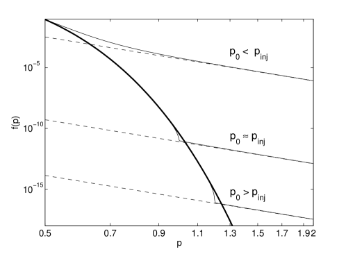
Figure 2: Shape of $f(p)$ for different values of $p_{0}$. Thin solid line represents $f(p)$, thick solid line - pure Maxwellian distribution, dashed line - power-law approximation.

3.3 The case of transitionless acceleration

If $p_{0}>p_{\rm inj}$, Eq. (44) is an appropriate solution for the distribution function. $\tilde{C}_{1}$ and $S_{N}$ are determined from the boundary conditions at $p=p_{0}$ and $p=p_{\rm max}$, namely, $f^{II}(p_{0})=f^{I}(p_{0})=f_{0}$ and $f^{II}(p_{\rm max})=0$,

$$S_{N} =\alpha(\varsigma+1)p_{0}^{\varsigma+1}f_{0}\,,$$ (52)

$$\tilde{C}_{1} =-{S_{N}p^{-(\varsigma+1)}_{\rm max}\over\alpha(\varsigma+1)}=-f_{0}\left({p_{\rm max}\over p_{0}}\right)^{-(\varsigma+1)}\,.$$ (53)

As $p_{\rm max}\gg p_{0}$, thus for simplicity we set $\tilde{C}_{1}=0$, and for non-relativistic temperatures $T\ll 1$ from Eq. (40) we have

$$f_{0}=\sqrt{\frac{2}{\pi}}\frac{N}{T^{3/2}}\exp\left(-{\mathcal{E}_{0}\over T}\right)\left[1+\frac{\alpha(\varsigma+1)p_{0}^{\varsigma+1}}{A(p_{0}^{2}+1)}\right]^{-1}\,.$$ (54)

In this case the run-away particle flux toward high energies can be expressed directly from Eq. (52) as

$$S_{N}=\alpha(\varsigma+1)p_{0}^{\varsigma+1}\sqrt{\frac{2}{\pi}}\frac{N}{T^{3/2}}\exp\left(-{\mathcal{E}_{0}\over T}\right)\left[1+\frac{\alpha(\varsigma+1)p_{0}^{\varsigma+1}}{A(p_{0}^{2}+1)}\right]^{-1}\,.$$ (55)

For $p_{0}\gg 1$ Eq. (3.2) becomes

$$W_{0}=\int\limits_{0}^{\infty}p^{2}\mathcal{E}f^{I}_{0}(p)dp=N\left[(3T-1)+{K_{1}(T^{-1})\over K_{2}(T^{-1})}\right]\,,$$ (56)

or for non-relativistic values of $T\ll 1$

$$W_{0}=\frac{3}{2}NT+\frac{15}{8}NT^{2}+\dots$$ (57)

Now we have (recall Eqs. (50) and (51))

$$\frac{\partial W_{0}}{\partial T}\frac{dT}{dt}=\left({W_{0}\over N}-\mathcal{E}_{0}\right)S_{N}+\int\limits_{p_{0}}^{\infty}\frac{p^{3}}{\sqrt{p^{2}+1}}\left[D_{0}(T)\frac{\partial f}{\partial p}-\left({dp\over dt}\right)_{0}f\right]\,dp$$ (58)

$$=\alpha f_{0}\mathcal{E}_{0}p_{0}^{\varsigma+1}(\varsigma+1)\left[\frac{AQ(p_{0},\varsigma)}{\alpha\mathcal{E}_{0}(\varsigma+1)}-1\right]+ATf_{0}\left\{\frac{3\alpha p_{0}^{\varsigma+1}(\varsigma+1)}{2A}-\left[1+\frac{(\varsigma+1)}{(\varsigma-1)}p_{0}^{2}\right]\right\}\,,$$

where

$$Q(p_{0},\varsigma)=\int\limits_{p_{0}}^{\infty}x^{-\varsigma}\sqrt{x^{2}+1\,}\,dx\,.$$ (59)

If $\alpha\mathcal{E}_{0}(\varsigma+1)\neq AQ(p_{0},\varsigma)$ and $\mathcal{E}_{0}\gg T$ then the second term in Eq.(58) is small and can be neglected. Finally from Eq. (57) we obtain

$$\frac{dT}{dt}=\frac{2S_{N}}{3N}\left[\frac{AQ(p_{0},\varsigma)}{\alpha(\varsigma+1)}-\mathcal{E}_{0}\right]\,,$$ (60)

where $A$ and $S_{N}$ are defined by Eqs. (25) and (55).

For high values of $\alpha$ one can see from Eq. (60) that the plasma cools down and $dT/dt<0$. The temperature decreases with time due to a very intensive outflow of high energy particles from the thermal pool, even though external sources in the form of stochastic Fermi acceleration supply energy to the system (analogue to Maxwell demon). This effect can be seen in Fig. 2 as a deficit of high energy thermal particles at $p<p_{0}$.

When $\alpha$ decreases, collisions start to dominate over the outflow effect. As the result the derivative $dT/dt$ increases and at sufficiently small $\alpha$ the regime changes from cooling to heating of plasma. However the process of acceleration reduces the amount of particles in the thermal pool ($dN/dt<0$ at $p<p_{0}$). If $\alpha$ remains constant then the value of $A$ decreases with time and, in principle for a sufficiently long time we come again to the condition when $\alpha\mathcal{E}_{0}(\varsigma+1)>A(t)Q(p_{0},\varsigma)$, enter the regime of plasma cooling again.

A more accurate analysis of this regime can be provided by numerical calculations of the nonlinear case.

4 Nonlinear Case: Semi-Analytical Method and Numerical Calculations

The most straightforward way to solve the problem is a numerical solution of the original nonlinear equation. However, this method is very time-consuming. We proceed with approximation methods that simplify the numerical calculations, but still give a good result.

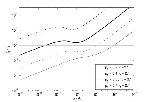
Figure 3: The comparison between heating timescale $t_{T}$ and tail-formation time-scale $t_{\rm F}$ for different $p_{0}$ and acceleration rates. The temperature is $T=0.016$ (the corresponding momentum is $p_{T}=0.12$). The threshold value is marked by the gray horizontal line.

Analysis of kinetic equations depend on the relation between the plasma heating time and the acceleration time. We define the heating time as

$$t_{T}=T/(dT/dt)\,.$$ (61)

The lower limit of this time can be obtained for the quasi-stationary solution for $dW/dt$ when we neglect the cooling term $S_{N}\mathcal{E}_{0}$ in Eq. (50). The acceleration time characterizes a period required for particles to fill the non-thermal tail. Numerical calculations show that for $\varsigma>2$ this time is of the order of

$$t_{\rm F}\simeq\alpha^{-1}\,.$$ (62)

The quasi-stationary state (when the plasma temperature is almost constant and the acceleration generate prominent non-thermal “tails”) can be reached only if $t_{T}>t_{\rm F}$. In this case we can use analytical solutions presented in previous section. The ratio $t_{T}/t_{\rm F}$ as a function of $p_{0}$ is shown in Fig. 3. The threshold value of ratio $t_{T}/t_{\rm F}=1$ is shown in Fig. 3 by the gray horizontal dashed line. The quasi-stationary state will be achieved if $t_{T}/t_{\rm F}$ is above the gray line.

If the acceleration time is larger than the heating time, $t_{T}<t_{\rm F}$, the quasi-stationary state cannot be reached. In this case we can simplify the calculations using the trick in Petrosian & East (2008). The evolution of distribution function $f(p)$ can be described by the non-stationary linear kinetic equation

$$\frac{\partial f}{\partial t}+\frac{1}{p^{2}}\frac{\partial}{\partial p}p^{2}\left[\left({dp\over dt}\right)_{0}(p,N,T)f-\left\{D_{0}(p,N,T)+D_{F}(p)\right\}\frac{\partial f}{\partial p}\right]=0\,.$$ (63)

We can estimate the variation of temperature by the following algorithm:

1. For a given $f(t,p)$, estimate $f(t+\delta t,p)$ from Eq. (63);

2. compute $N(t+\delta t)$ from $\int_{0}^{\infty}f(t+\delta t,p)dp$;

3. calculate $\dot{W_{0}}$ from Eq. (50), then $W_{0}(t+\delta t)=W_{0}(t)+\dot{W_{0}}\delta t$, then find $T(t+\delta t)$ from Eq. (3.2);

4. for new values of $N(t+\delta t)$ and $T(t+\delta t)$ recalculate the kinetic coefficients using analytical expressions for Maxwellian coefficients, see Eqs. (64) & (65);

5. repeat steps 1-4.

The analytical expressions for the kinetic coefficients are calculated as (see Petrosian & East, 2008, and references therein):

$$\left({dp\over dt}\right)_{0}(p,N,T)=-\,\frac{A(p^{2}+1)}{p^{2}}\left[\mbox{erf}\left(\sqrt{{\mathcal{E}\over T}}\right)-\sqrt{{4\mathcal{E}\over\pi T}}\exp\left(-{\mathcal{E}\over T}\right)\right]\,,$$ (64)

$$D_{0}(p,N,T)=-\,{T\sqrt{p^{2}+1}\over p}\left({dp\over dt}\right)_{0}(p,N,T)\,.$$ (65)

Here $\mbox{erf}(z)$ is the error function.

With this method we combine the simplicity of the analytical method with the accuracy of the numerical method. The only problem is that this approach like any other semi-analytical method based on Eq. (50) cannot be used near $p_{0}=0$.

Now we compare the results obtained with different methods. We consider the following methods:

1. Transitionless case: It is based on Eq. (60). The equations are integrated numerically using the Runge-Kutta method to obtain the evolution of the temperature $T(t)$ and density $N(t)$. This method is applicable if $p_{\rm inj}<p_{0}$.

2. Quasi-linear approximation: The distribution function is given as in Eq. (41) and (3.1). Eqs. (50) and (3.2) are used to estimate the $dT/dt$. The variations of the temperature $T(t)$ and density $N(t)$ are obtained using the Runge-Kutta method. This approximation is valid for $t_{T}>t_{\rm F}$.

3. Semi-analytical method: It uses a combination of numerical solution to Eq. (63) and analytical calculations of Eqs. (50) & (3.2) in order to estimate the variations of the temperature. This method can be applied to $p_{0}\gg p_{T}=\sqrt{(T+1)^{2}-1}$.

4. Numerical method: Evolution of the distribution function is obtained by a numerical solution of the original non-linear equation Eq. (7) (for details see Appendix B). This method is the most universal and is used to check whether the results obtained by methods 1-3 are correct.

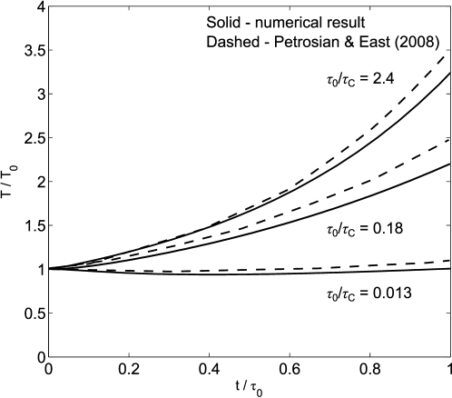
Figure 4: Comparison between our numerical method (solid line) and method used by Petrosian & East (2008) (dashed line). All notations are the same as in Petrosian & East (2008) (see the text for details).

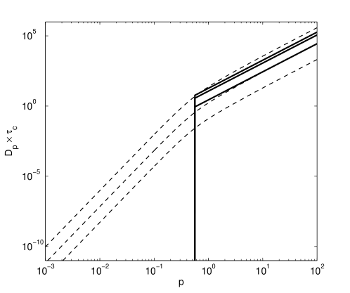
Figure 5: Comparison between $D_{F}(p)$ used by Petrosian & East (2008) (thin dashed lines), Eq. (15), and in this paper (thick solid lines), Eq. (17).

We checked our numerical program by calculations of temperature variations for the acceleration in the form Eq. (15) and for the same parameters as used by Petrosian & East (2008), i.e., $p_{0}=0$, $q=1$, $\mathcal{E}_{c}=0.2$ and three values of $\tau_{0}$ equaled correspondingly: $2.4\tau_{C}$, $0.18\tau_{C}$ and $0.013\tau_{C}$, where $\tau_{C}\equiv(4\pi r_{0}^{2}cN\ln\Lambda)^{-1}\approx 2.7\times 10^{7}\times(N/10^{-3}~{}\mbox{cm}^{-3})^{-1}$ yr and $r_{0}=e^{2}/(m_{e}c^{2})$. The acceleration parameters, $D_{F}(p)$, for these three cases are shown in Fig. 5 by the thin dashed lines.

The result of our calculations and that of Petrosian & East (2008) are shown in Fig. 4 by the solid and dashed lines correspondingly. One can see that despite of some discrepancy the results are more or less the same.

Now we present results of calculations for the acceleration parameter $D_{F}$ in the form (17), when $p_{0}\neq 0$. In all cases we take $p_{0}=0.55$. Variations of $p_{0}$ change the temperature variations quantitatively but not qualitatively. We choose $\varsigma=2$ in order to obtain the same momentum dependence of $D_{F}$ at high energies as in Eq. (15). Note that in this case $t_{\rm F}=2\tau_{0}$. Below we will use $\tau_{0}$ as a characteristic timescale to compare results with those of Petrosian & East (2008).

For other values of $\varsigma$ the results are qualitatively the same, yet lower values of $\varsigma$ will increase the amount of non-thermal particles and thus decrease the heating timescale and vice-versa. One can see this from Eq. (60).

The calculations where performed for the three different regimes of acceleration:

• heating dominates over cooling;

• cooling and heating rates are of the same order;

• cooling dominates over heating.

The functions $D_{F}(p)$ used for these three cases are shown in Fig. 5 by the solid lines.

We provide calculations by the four different methods: analytical (transitionless), quasi-linear, semi-analytical and numerical. Temperature variations, $T(t)$, obtained by these methods are shown in Figs. 6, 8 and 9 by the dashed, thin solid, thick solid and dotted lines, correspondingly.

• For the case of slow acceleration we take $\alpha/A=2.77$. In this case the quasi-stationary approach is not valid, and only numerical and semi-analytical methods can provide an adequate result. Temperature variations for this case of acceleration parameter are shown in Fig. 6. As one can see the result of acceleration for this parameter $\alpha$ is the plasma overheating that is in complete agreement with the conclusions of Wolfe & Melia (2006) and Petrosian & East (2008). The only difference is that the overheating occurs for the time $t\approx 4.5\tau_{0}\approx 1.6\tau_{C}$ which is longer than that of Petrosian & East (2008) by a factor of 4 who obtained $t\sim\tau_{0}$. The reason is that for $p_{0}=0$ the acceleration generates an extended excess above the equilibrium Maxwellian function while for $p_{0}\neq 0$ this excess is not so prominent (compare dashed and solid lines in Fig. 7). Since the amount of suprathermal particles in the case $p_{0}=0$ is higher than the case $p_{0}>0$, it is not surprising that the plasma is overheated by the Coulomb losses in a shorter time when $p_{0}=0$.

  

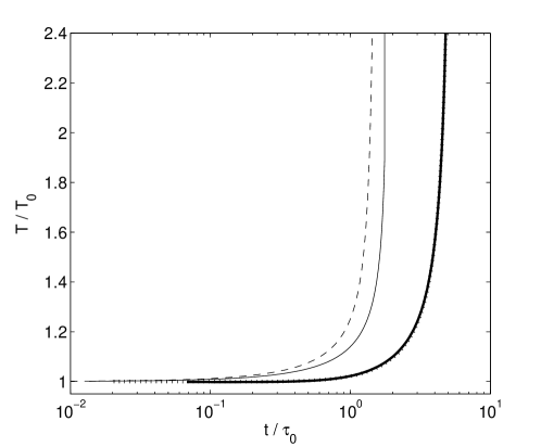
  Figure 6: The temperature evolution when heating dominates over cooling for the parameters: $\alpha/A=2.77$, $p_{0}=0.55$, $\varsigma=2$, $T_{0}=7$ keV. Dotted line - numerical model, thick solid line - semi-analytical model, thin solid line - quasi-linear model, dashed line - transitionless model. Note that semi-analytical model and the numerical model almost overlap entirely.

  

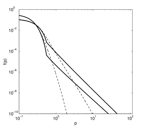
  Figure 7: Comparison between spectra formed under influence of momentum diffusion coefficient in the form of Eq. (15) for $\tau_{0}=0.18\tau_{C}$ (thin dashed lines) and those of Eq. (17) for $\alpha/A=2.77$, $\varsigma=2$ and $p_{0}=0.55$ (solid lines). The distribution were taken at the moment when the temperatures are the same. Two values of the temperature were used: $T_{1}=8.5$ keV, $T_{2}=16.5$ keV.

• The case of moderate acceleration ($\alpha/A=11.63$) is shown in Fig. 8. One can see that all methods are in good agreement. At the first stage we see plasma heating, however the timescale is much longer than in Petrosian & East (2008), the plasma temperature increases by a factor of 1.3 at the moment $t\approx 86\tau_{0}=7\tau_{C}$ that is almost two orders of magnitude higher than that of Petrosian & East (2008). A prominent quasi-stationary power-law tail of nonthermal particles is formed by the acceleration for a much shorter time (since $t_{T}/t_{\rm F}>1$, see Fig. 3). Moreover unlike in Petrosian & East (2008), after this time heating reverses to cooling.

• The case of fast acceleration ($\alpha/A=18.5$) is shown in Fig. 9. The numerical method, the semi-analytical method and the quasi-linear approximation give almost the same result. For comparison we also show the calculations obtained with transitionless case (dashed line). We see that in spite of some difference this method provides a similar qualitative time variations of the temperature $T$. All methods demonstrate plasma cooling in this regime from the very beginning. The temperature of the plasma shows a steady decrease with time while nonthermal tails are formed rapidly ($t_{T}/t_{\rm F}>1$, see Fig. 3) that differs completely from the results obtained by Petrosian & East (2008).

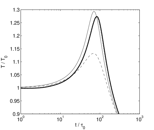
Figure 8: Same as Fig. 6 but for the case when cooling and heating processes are of the same order of magnitude ($\alpha/A=11.6$).

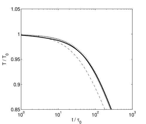
Figure 9: Same as Fig. 6 but for the case when cooling dominates over heating ($\alpha/A=18.5$).

These results can be understood from Fig. 2. For the ratio $\alpha/A=2.77$ the injection momentum is $p_{\rm inj}\simeq 0.83$, i.e., $p_{\rm inj}>p_{0}$ (similar to the upper curve of Fig. 2). An excess of quasi-thermal particles is formed in the range between $p_{0}$ and $p_{\rm inj}$. Coulomb losses of these particles results in effective plasma heating. As we already above-mentioned Petrosian & East (2008) assumed $p_{0}=0$ that led to more extended transition region and more effective heating.

In the case of $\alpha/A=11.63$, $p_{\rm inj}\simeq 0.5\simeq p_{0}$ (similar to the middle curve of Fig. 2). The transition region is almost negligible in this case. Therefore, plasma heating by nonthermal particles is insignificant which then changes into cooling.

In the case of $\alpha/A=18.5$, $p_{\rm inj}\simeq 0.4$, i.e., $p_{\rm inj}<p_{0}$ (similar to the lower curve of Fig. 2). A deficit of high energy particles is formed in the thermal energy range that provides the effect of cooling.

Thus, we conclude, that depending on parameters, $p_{0}$ and $\alpha$, different regimes of acceleration from background plasma are realized. The important inference is that stochastic acceleration may produce a flux of nonthermal particle without plasma overheating.

A specific spectrum of turbulence that provides stochastic acceleration is out of the scope of this paper. It depends on mechanisms which excite electromagnetic fluctuations in an astrophysical plasma. As an example, we mention particle acceleration in OB-associations by a supersonic turbulence (see Bykov & Toptygin, 1993). The momentum diffusion coefficient in this case has the form $D(p)=D_{0}p^{2}$. This acceleration is effective in the momentum range $p>p_{0}$, where the value of $p_{0}$ is derived from $r_{L}(p_{0})=lu/c$. Here $r_{L}$ is the particle Larmor radius, $u$ is the shock velocity and $l$ is a distance between shocks. Particles with $p<p_{0}$ are not accelerated by this mechanism.

5 Conclusion

We analyzed nonlinear kinetic equations describing particle stochastic (or second-order Fermi) acceleration from background plasma when the acceleration is non-zero for particles with momenta $p>p_{0}$. The goal of these investigations is to define whether the only result of stochastic acceleration is plasma overheating as concluded by Wolfe & Melia (2006) and Petrosian & East (2008), or this acceleration can generate prominent tails of nonthermal particles when the plasma temperature remains almost stationary. The following results are obtained from our analysis:

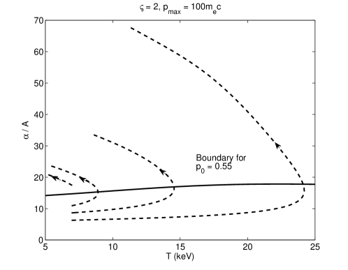
Figure 10: Regions of heating (below the solid line) and cooling (above the solid line) in the parameter space ($T,\alpha/A$). The dashed lines show the evolution of systems at the same starting temperature but with different $\alpha/A$.

1. We showed that in the case of stochastic acceleration two competitive processes determine temperature variations of background plasma. The first one is Coulomb energy losses of nonthermal particles which heat the plasma. The other one is a run-away flux of high-energy particles from the thermal pool that leads to plasma cooling. Depending on the rates of these processes the plasma may cool down or heat up.

2. From numerical and analytical calculations we conclude that for a low enough acceleration rate the cooling process is negligible. The plasma gains much heat on the acceleration timescale $\tau_{0}$. As a result the plasma temperature rises rapidly while prominent nonthermal tails are not generated, that fully confirms results of Wolfe & Melia (2006) and Petrosian & East (2008).

3. For a moderate acceleration the cooling and heating processes partly compensate each other. As a results the plasma temperature is quasi-stationary on a timescales much longer than $\tau_{0}$. In this case, the acceleration produces a nonthermal component of the spectrum. After a period of moderate plasma heating the process changes into cooling. This regime does not appear in the models of Wolfe & Melia (2006) and Petrosian & East (2008).

4. For a high rate of acceleration the run-away flux of thermal particles cools the plasma down from the very beginning. In spite of energy supply by external sources the plasma temperature drops down (analogue to Maxwell demon).

5. The evolution of plasma temperature depends on the characteristic time of Coulomb collisions in the background plasma (the collision frequency $A$) and the acceleration frequency $\alpha$. This is illustrated in Fig. 10 where the solid line defines the border between heating (below the line) and cooling (above the line) regimes for quasi-stationary systems. It corresponds to the solution of the $dT/dt=0$ (see Eq. (50)). Dashed lines in Fig. 10 show the evolution of plasma parameters for the same initial temperature but different initial value of $A$ ($\alpha$ is the same for the systems). Since $N$ decreases monotonically because of particle acceleration, $A$ decreases monotonically accordingly (see Eq. (25)).

   One can see that even if the system starts from the regime of heating, sooner or later it changes to plasma cooling. If the evolution of the system is quasi-stationary the turning point of the trajectory should be located on the boundary. However we mention that the quasi-stationary approximation is inapplicable to low values of $\alpha/A$.

Appendix A General Kinetic Equation

The general equation for stochastic Fermi acceleration with the coefficient $D^{F}_{\alpha\beta}$ the equation has the form (Landau & Lifshitz, 1981; Wolfe & Melia, 2006)

$$\frac{\partial f({\bf p})}{\partial t}=\frac{\partial}{\partial p_{\alpha}}\left[\left(D_{\alpha\beta}+D^{F}_{\alpha\beta}\right)\frac{\partial f({\bf p})}{\partial p_{\beta}}-F_{\alpha}f({\bf p})\right]\,,$$ (A1)

where ${\bf p}={\bf v}\left(c^{2}-{\bf v}^{2}\right)^{-1/2}$ is the dimensionless particle momentum and ${\bf v}$ is the particle velocity. The coefficients $D_{\alpha\beta}$ and $F_{\alpha}$ are determined by Coulomb collisions of the particles,

$$D_{\alpha\beta}=A\int Z_{\alpha\beta}({\bf p},{\bf p^{\prime}})f({\bf p^{\prime}})d^{3}p^{\prime}\,,\quad F_{\alpha}=-A\int\left[\frac{\partial}{\partial p^{\prime}_{\beta}}Z_{\alpha\beta}({\bf p},{\bf p^{\prime}})\right]f({\bf p^{\prime}})d^{3}p^{\prime}\,,$$ (A2)

where

$$Z_{\alpha\beta}({\bf p},{\bf p^{\prime}})=\frac{r^{2}}{\gamma\gamma^{\prime}w^{3}}\left[w^{2}\delta_{\alpha\beta}-p_{\alpha}p_{\beta}-p^{\prime}_{\alpha}p^{\prime}_{\beta}+r(p_{\alpha}p^{\prime}_{\beta}+p^{\prime}_{\alpha}p_{\beta})\right]\,,$$ (A3)

$$A=\frac{8\pi e^{2}e^{\prime\,2}\ln\Lambda}{m^{2}}\,,\quad r=\gamma\gamma^{\prime}-{\bf p\cdot p^{\prime}}/c^{2}\,,\quad w=c\sqrt{r^{2}-1}\,,\quad\gamma=\sqrt{1+{\bf p}^{2}/c^{2}}\,.$$ (A4)

The boundary conditions were taken in the form: a zero particle flux at $p=0$:

$$\left[\left(D_{\alpha\beta}+D^{F}_{\alpha\beta}\right)\frac{\partial f({\bf p})}{\partial p_{\beta}}-F_{\alpha}f({\bf p})\right]_{p=0}=0\,,$$ (A5)

and the distribution function vanishes at some $p_{\rm max}$:

$$f({\bf p}_{\rm max})=0\,.$$ (A6)

Appendix B Numerical Method for the Nonlinear Case

To solve Eq. (7) numerically we use the Crank-Nicolson finite difference method. To estimate the kinetic coefficients (A2) we use Simpson’s integration rule,

$${\bf D}={\bf\mathcal{Z}f}\,,\quad{\bf F}={\bf\mathcal{Z^{\prime}}f}\,,$$ (B1)

where vectors ${\bf f}$, ${\bf D}$ and ${\bf F}$ are corresponding discrete versions of $f(p)$, $D_{c}(p,f)$ and $(dp/dt)_{c}(p,f)$. Matrices ${\bf\mathcal{Z}}$ and ${\bf\mathcal{Z^{\prime}}}$ are obtained by applying Simpson’s rule to Eq. (A2). The discrete version of Eq. (7) at $t=(t_{n}+t_{n+1})/2$ and $p=p_{j}$ looks like (see e.g., Park & Petrosian (1996) and references therein)

$$\frac{f_{n+1,j}-f_{n,j}}{\Delta t}=\frac{1}{p_{j}^{2}}\frac{S_{n+{\scriptstyle{1\over 2}},j+{\scriptstyle{1\over 2}}}-S_{n+{\scriptstyle{1\over 2}},j-{\scriptstyle{1\over 2}}}}{\Delta p_{j}}\,,$$ (B2)

where $\Delta t=t_{n+1}-t_{n}$ and $\Delta p_{j}=(p_{j+1}-p_{j-1})/2$ are steps of the grid and the flux is expressed according to the Crank-Nicolson rule:

$$S_{n+{\scriptstyle{1\over 2}},j+{\scriptstyle{1\over 2}}} ={\textstyle{1\over 2}}p_{j}^{2}\left[D_{n+1,j+{\scriptstyle{1\over 2}}}\frac{f_{n+1,j+1}-f_{n+1,j}}{\Delta p_{j+{\scriptstyle{1\over 2}}}}-F_{n+1,j+{\scriptstyle{1\over 2}}}f_{n+1,j+{\scriptstyle{1\over 2}}}\right]+$$

$$\quad+{\textstyle{1\over 2}}p_{j}^{2}\left[D_{n,j+{\scriptstyle{1\over 2}}}\frac{f_{n,j+1}-f_{n,j}}{\Delta p_{j+{\scriptstyle{1\over 2}}}}-F_{n,j+{\scriptstyle{1\over 2}}}f_{n,j+{\scriptstyle{1\over 2}}}\right]\,,$$

$$D_{n,j+{\scriptstyle{1\over 2}}} ={\textstyle{1\over 2}}(D_{n,j}+D_{n,j+1})\,,$$ (B4)

$$F_{n,j+{\scriptstyle{1\over 2}}} ={\textstyle{1\over 2}}(F_{n,j}+F_{n,j+1})\,,$$ (B5)

$$f_{n,j+{\scriptstyle{1\over 2}}} ={\textstyle{1\over 2}}(f_{n,j}+f_{n,j+1})\,,$$ (B6)

$$\Delta p_{j+{\scriptstyle{1\over 2}}} =p_{j+1}-p_{j}\,.$$ (B7)

The boundary condition at $p=0$ imply that $S_{n+{\scriptstyle{1\over 2}},-{\scriptstyle{1\over 2}}}=0$. The boundary condition at $p=p_{\rm max}$ is $f(p_{\rm max})=0$.

After discretization we arrive at the non-linear system of equations,

$${\bf f_{n+1}}-{\bf f_{n}}=\mathcal{A}({\bf f_{n+1}}){\bf f_{n+1}}+\mathcal{A}({\bf f_{n}}){\bf f_{n}}\,,$$ (B8)

where ${\bf\mathcal{A}(f)}$ is a tridiagonal matrix corresponding to the differential operator in RHS of Eq. (B2). According to Eq. (B1), ${\bf\mathcal{A}(f)}$ is a linear function of ${\bf f}$ and Eq. (B8) is a system of quadratic equations.

To avoid calculations of Jacobian matrix we do not apply Newton’s method and utilize a simple iteration method instead. However the iteration method based on Eq. (B8) converges very slowly. We rewrite the iteration step in the following form

$${\bf\left(E-\mathcal{A}(f^{k}_{n+1})\right)f^{k+1}_{n+1}}=\mathcal{A}({\bf f_{n}}){\bf f_{n}}+{\bf f_{n}}\,,$$ (B9)

where $k$ is the number of iteration and ${\bf E}$ is a unit matrix. The system of linear equations is solved using tridiagonal matrix algorithm. Iteration in the form Eq. (B9) shows fast convergence if the temperature of the Maxwellian distribution does not change significantly between $t_{n}$ and $t_{n+1}$.

Since the Crank-Nicolson method may be affected by numerical oscillations we also use less precise and more robust backward Euler method (simple fully implicit method from Park & Petrosian, 1996). The backward Euler method turns out to be useful for non-thermal tails of low magnitude when the value of $\alpha$ is low and the value of $p_{0}$ is high.

The discretization in momentum space is tricky since we need to provide a good resolution for Maxwellian distribution and transitional region as well as calculate the nonthermal tail at high energies. We tried two possible ways to reduce the number of grid points. The first one is to split the momentum axis into sub-domains and join them using continuity of the distribution function and particle flux. The second way is to use the logarithmic grid by introducing new variable $q=\log(p)$. Both methods gives almost the same results.

References

- Ajello et al. (2010) Ajello, M., Rebusco, P., Cappelluti N. et al. 2010, ApJ , 725, 1688
- Berezinskii et al. (1990) Berezinskii, V. S., Bulanov, S. V., Dogiel, V. A., Ginzburg, V. L., & Ptuskin, V. S. 1990, Astrophysics of Cosmic Rays, ed. V.L.Ginzburg, (Norht-Holland, Amsterdam)
- Bykov & Toptygin (1993) Bykov, A. M. & Toptygin, I. N. 1993, Physics Uspekhi, 36, 1020
- Cheng et al. (2011) Cheng, K.-S., Chernyshov, D. O., Dogiel, V. A., Ko, C.-M., & Ip, W.-H. 2011, ApJ, 731, L17
- Dogiel (2000) Dogiel, V. A. 2000, A&A, 357, 66
- Dogiel et al. (2007) Dogiel, V. A., Colafrancesco, S., Ko, C.-M. et al. 2007, A&A, 461, 443
- Eckert et al. (2008) Eckert, D., Produit, N., Paltani, S. et al. 2008, A&A, 479, 27
- Enßlin et al. (1999) Enßlin, T. A., Lieu, R., & Bierman, P. L. 1999, A&A, 344, 409
- Fermi (1949) Fermi, E. 1949, PhRv, 75, 1169
- Fermi (1954) Fermi, E. 1954, ApJ, 119, 1
- Fusco-Femiano et al. (1999) Fusco-Femiano, R., dal Fiume, D., Feretti L. et al. 1999, ApJL, 513, L21
- Fusco-Femiano et al. (2007) Fusco-Femiano, R., Landi, R. & Orlandini M. 2007, ApJL, 654, L9
- Gurevich (1960) Gurevich, A. V. 1960, Sov. Phys. JETP, 38, 1150
- Landau & Lifshitz (1981) Landau, L., & Lifshitz, E. 1981, Physical Kinetics (Oxford: Pergamon Press)
- Liang et al. (2002) Liang, H., Dogiel, V. A., & Birkinshaw, M. 2002, MNRAS, 337, 567
- MacDonald et al. (1957) MacDonald, W. M., Rosenbluth, M. N., & Wong, C. 1957, PhRv, 107, 350
- Mertsch & Sarkar (2011) Mertsch, Ph., & Sarkar, S. 2011, PhRvL, 107, 091101
- Miller et al. (1990) Miller, J. A., Guessoum, N., & Ramaty, R. 1990, ApJ, 361, 701
- Nayakshin & Melia (1998) Nayakshin, S., & Melia, F. 1998, ApJS, 114, 269
- Nevalainen (2009) Nevalainen, J., Eckert, D., Kaastra, J. et al. 2009, A&A, 508, 1161
- Park & Petrosian (1996) Park, B.T., & Petrosian, V. 1996, ApJS, 103, 255
- Petrosian (2001) Petrosian, V. 2001, ApJ, 557, 560
- Petrosian & East (2008) Petrosian, V. & East, W.E. 2008, ApJ, 682, 175
- Petrosian (2012) Petrosian, V., 2012, arXiv:1205.2136
- Rephaeli et al. (1999) Rephaeli, Y., Gruber, D., & Blanco P. 1999, ApJL, 511, L21
- Rephaeli et al. (2008) Rephaeli, Y., Nevalainen, J., Ohashi, T. & Bykov A. M. 2008, Space Science Reviews, 134, 71
- Toptygin (1985) Toptygin I.N. 1985, it Cosmic rays in interplanetary magnetic fields, Dordrecht, D. Reidel Publishing Co.
- Wolfe & Melia (2006) Wolfe, B., & Melia, F. 2006, ApJ, 638, 125
- Wolfe & Melia (2008) Wolfe, B., & Melia, F. 2008, ApJ, 675, 156