Efficient implementation of Markov chain Monte Carlo when using an unbiased likelihood estimator

Efficient implementation of Markov chain Monte Carlo when using an unbiased likelihood estimator

Abstract

When an unbiased estimator of the likelihood is used within a Metropolis–Hastings chain, it is necessary to trade off the number of Monte Carlo samples used to construct this estimator against the asymptotic variances of averages computed under this chain. Many Monte Carlo samples will typically result in Metropolis–Hastings averages with lower asymptotic variances than the corresponding Metropolis–Hastings averages using fewer samples. However, the computing time required to construct the likelihood estimator increases with the number of Monte Carlo samples. Under the assumption that the distribution of the additive noise introduced by the log-likelihood estimator is Gaussian with variance inversely proportional to the number of Monte Carlo samples and independent of the parameter value at which it is evaluated, we provide guidelines on the number of samples to select. We demonstrate our results by considering a stochastic volatility model applied to stock index returns.

Keywords: Intractable likelihood, Metropolis-Hastings algorithm, Particle filter, Sequential Monte Carlo, State-space model.

1 Introduction

The use of unbiased estimators within the Metropolis–Hastings algorithm was initiated by Lin et al. (2000), with a surge of interest in these ideas since their introduction in Bayesian statistics by Beaumont (2003). In a Bayesian context, an unbiased likelihood estimator is commonly constructed using importance sampling as in Beaumont (2003) or particle filters as in Andrieu et al. (2010). Andrieu & Roberts (2009) call this method the pseudo-marginal algorithm, and establish some of its theoretical properties.

Apart from the choice of proposals inherent to any Metropolis–Hastings algorithm, the main practical issue with the pseudo-marginal algorithm is the choice of the number, $N$, of Monte Carlo samples or particles used to estimate the likelihood. For any fixed $N$, the transition kernel of the pseudo-marginal algorithm leaves the posterior distribution of interest invariant. Using many Monte Carlo samples usually results in pseudo-marginal averages with asymptotic variances lower than the corresponding averages using fewer samples, as established by Andrieu & Vihola (2014) for likelihood estimators based on importance sampling. Empirical evidence suggests this result also holds when the likelihood is estimated by particle filters. However, the computing cost of constructing the likelihood estimator increases with $N$. We aim to select $N$ so as to minimize the computational resources necessary to achieve a specified asymptotic variance for a particular pseudo-marginal average. This quantity, which is referred to as the computing time, is typically proportional to $N$ times the asymptotic variance of this average, which is itself a function of $N$. Assuming that the distribution of the additive noise introduced by the log-likelihood estimator is Gaussian, with a variance inversely proportional to $N$ and independent of the parameter value at which it is evaluated, this minimization was carried out in Pitt et al. (2012) and in Sherlock et al. (2013). However, Pitt et al. (2012) assume that the Metropolis–Hastings proposal is the posterior density, whereas Sherlock et al. (2013) relax the Gaussian noise assumption, but restrict themselves to an isotropic normal random walk proposal and assume that the posterior density factorizes into $d$ independent and identically distributed components and $d\rightarrow\infty$.

Our article addresses a similar problem but considers general proposal and target densities and relaxes the Gaussian noise assumption. In this more general setting, we cannot minimize the computing time, and instead minimize explicit upper bounds on it. Quantitative results are presented under a Gaussian assumption. In this scenario, our guidelines are that $N$ should be chosen such that the standard deviation of the log-likelihood estimator should be around $1.0$ when the Metropolis–Hastings algorithm using the exact likelihood is efficient and around $1.7$ when it is inefficient. In most practical scenarios, the efficiency of the Metropolis–Hastings algorithm using the exact likelihood is unknown as it cannot be implemented. In these cases, our results suggest selecting a standard deviation around $1.2$.

2 Metropolis–Hastings method using an estimated likelihood

We briefly review how an unbiased likelihood estimator may be used within a Metropolis–Hastings scheme in a Bayesian context. Let $y\in\mathsf{Y}$ be the observations and $\theta\in\Theta\subseteq\mathbb{R}^{d}$ the parameters of interest. The likelihood of the observations is denoted by $p(y\mid\theta)$ and the prior for $\theta$ admits a density $p(\theta)$ with respect to Lebesgue measure so the posterior density of interest is $\pi(\theta)\propto p(y\mid\theta)p(\theta)$. We slightly abuse notation by using the same symbols for distributions and densities.

The Metropolis–Hastings scheme to sample from $\pi$ simulates a Markov chain according to the transition kernel

$$Q_{\textsc{ex}}\left(\theta,\mathrm{d}\vartheta\right)=q\left(\theta,\vartheta\right)\alpha_{\textsc{ex}}(\theta,\vartheta)\mathrm{d}\vartheta+\left\{1-\varrho_{\textsc{ex}}\left(\theta\right)\right\}\delta_{\theta}\left(\mathrm{d}\vartheta\right),$$ (1)

where

$$\alpha_{\textsc{ex}}(\theta,\vartheta)=\min\{1,r_{\textsc{ex}}(\theta,\vartheta)\}\text{, \ \ }\varrho_{\textsc{ex}}\left(\theta\right)=\int q\left(\theta,\vartheta\right)\alpha_{\textsc{ex}}(\theta,\vartheta)\mathrm{d}\vartheta,$$ (2)

with $r_{\textsc{ex}}(\theta,\vartheta)=\pi(\vartheta)q\left(\vartheta,\theta\right)/\left\{\pi(\theta)q\left(\theta,\vartheta\right)\right\}$. This Markov chain cannot be simulated if $p(y\mid\theta)$ is intractable.

Assume $p(y\mid\theta)$ is intractable, but we have access to a non-negative unbiased estimator $\widehat{p}(y\mid\theta,U)$ of $p(y\mid\theta)$, where $U\sim m\left(\cdot\right)$ represents all the auxiliary random variables used to obtain this estimator. In this case, we introduce the joint density $\overline{\pi}(\theta,u)$ on $\Theta\times\mathcal{U}$, where

$$\overline{\pi}(\theta,u)=\pi(\theta)m(u)\widehat{p}(y\mid\theta,u)/p(y\mid\theta).$$ (3)

This joint density admits the correct marginal density $\pi(\theta)$, because $\widehat{p}(y\mid\theta,U)$ is unbiased. The pseudo-marginal algorithm is a Metropolis–Hastings scheme targeting (3) with proposal density $q\left(\theta,\cdot\right)m\left(\cdot\right)$, yielding the acceptance probability

$$\min\left\{1,\frac{\widehat{p}(y\mid\vartheta,v)p\left(\vartheta\right)q\left(\vartheta,\theta\right)}{\widehat{p}(y\mid\theta,u)p\left(\theta\right)q\left(\theta,\vartheta\right)}\right\}=\min\left\{1,\frac{\widehat{p}(y\mid\vartheta,v)/p(y\mid\vartheta)}{\widehat{p}(y\mid\theta,u)/p(y\mid\theta)}r_{\textsc{ex}}(\theta,\vartheta)\right\},$$ (4)

for a proposal $\left(\vartheta,v\right)$. In practice, we only record $\left\{\theta,\log\widehat{p}(y\mid\theta,u)\right\}$ instead of $\left\{\theta,u\right\}$. We follow Andrieu & Roberts (2009) and Pitt et al. (2012) and analyze this scheme using additive noise, $Z=\log\widehat{p}(y\mid\theta,U)-\log p(y\mid\theta)=\psi(\theta,U)$, in the log-likelihood estimator, rather than $U$. In this parameterization, the target density on $\Theta\times\mathbb{R}$ becomes

$$\overline{\pi}(\theta,z)=\pi(\theta)\exp\left(z\right)g(z\mid\theta),$$ (5)

where $g(z\mid\theta)$ is the density of $Z$ when $U\sim m(\cdot)$ and the transformation $Z=\psi(\theta,U)$ is applied.

To sample from $\overline{\pi}(\theta,z)$, we could use the scheme previously described to sample from $\overline{\pi}(\theta,u)$ and then set $z=\psi(\theta,u)$. We can equivalently use the transition kernel

$$Q\left\{\left(\theta,z\right),\left(\mathrm{d}\vartheta,\mathrm{d}w\right)\right\} =q\left(\theta,\vartheta\right)g(w\mid\vartheta)\alpha_{Q}\left\{\left(\theta,z\right),\left(\vartheta,w\right)\right\}\mathrm{d}\vartheta\mathrm{d}w$$ (6)

$$\text{ \ \ \ \ \ \ \ \ \ \ \ \ \ \ \ \ \ \ \ \ \ }+\left\{1-\varrho_{Q}\left(\theta,z\right)\right\}\delta_{\left(\theta,z\right)}\left(\mathrm{d}\vartheta,\mathrm{d}w\right),$$

where

$$\alpha_{Q}\left\{\left(\theta,z\right),\left(\vartheta,w\right)\right\}=\min\{1,\exp(w-z)\text{ }r_{\textsc{ex}}(\theta,\vartheta)\}$$ (7)

is (4) expressed in the new parameterization. Henceforth, we make the following assumption.

Assumption 1.

The noise density is independent of $\theta$ and is denoted by $g\left(z\right)$.

Under this assumption, the target density (5) factorizes as $\pi(\theta)\pi_{\textsc{z}}\left(z\right)$, where

$$\pi_{\textsc{z}}\left(z\right)=\exp\left(z\right)g(z).$$ (8)

Assumption 1 allows us to analyze in detail the performance of the pseudo-marginal algorithm. This simplifying assumption is not satisfied in practical scenarios. However, in the stationary regime, we are concerned with the noise density at values of the parameter which arise from the target density $\pi\left(\theta\right)$ and the marginal density of the proposals at stationarity $\int\pi\left(\mathrm{d}\vartheta\right)q\left(\vartheta,\theta\right)$. If the noise density does not vary significantly in regions of high probability mass of these densities, then we expect this assumption to be a reasonable approximation. In Section 4, we examine experimentally how the noise density varies against draws from $\pi\left(\theta\right)$ and $\int\pi\left(\mathrm{d}\vartheta\right)q\left(\vartheta,\theta\right)$.

3 Main results

3.1 Outline

This section presents the main contributions of the paper. All the proofs are in Appendix 1 and in the Supplementary Material. We minimize upper bounds on the computing time of the pseudo-marginal algorithm, as discussed in Section 1. This requires establishing upper bounds on the asymptotic variance of an ergodic average under the kernel $Q$ given in (6). To obtain these bounds, we introduce a new Markov kernel $Q^{\ast}$, where

$$Q^{\ast}\left\{\left(\theta,z\right),\left(\mathrm{d}\vartheta,\mathrm{d}w\right)\right\} =q\left(\theta,\vartheta\right)g(w)\alpha_{Q^{\ast}}\left\{\left(\theta,z\right),\left(\vartheta,w\right)\right\}\mathrm{d}\vartheta\mathrm{d}w$$ (9)

$$\text{ \ \ \ \ \ \ \ \ \ \ \ \ }+\left\{1-\varrho_{\textsc{ex}}\left(\theta\right)\varrho_{\textsc{z}}\left(z\right)\right\}\delta_{\left(\theta,z\right)}\left(\mathrm{d}\vartheta,\mathrm{d}w\right),$$

and

$$\alpha_{Q^{\ast}}\left\{\left(\theta,z\right),\left(\vartheta,w\right)\right\} =\alpha_{\textsc{ex}}(\theta,\vartheta)\alpha_{\textsc{z}}(z,w)\text{, \ \ }\alpha_{\textsc{z}}\left(z,w\right)=\min\{1,\exp(w-z)\},$$ (10)

$$\varrho_{\textsc{z}}\left(z\right) =\int g\left(w\right)\alpha_{\textsc{z}}\left(z,w\right)\mathrm{d}w.$$ (11)

As $Q$ and $Q^{\ast}$ are reversible with respect to $\overline{\pi}$ and the acceptance probability (10) is always smaller than (7), an application of the theorem in Peskun (1973) ensures that the variance of an ergodic average under $Q^{\ast}$ is greater than or equal to the variance under $Q$. We obtain an exact expression for the variance under the bounding kernel $Q^{\ast}$ and simpler upper bounds by exploiting a non-standard representation of this variance, the factor form of the acceptance probability (10) and the spectral properties of an auxiliary Markov kernel.

3.2 Inefficiency of Metropolis–Hastings type chains

This section recalls and establishes various results on the integrated autocorrelation time of Markov chains, henceforth referred to as the inefficiency. In particular, we present a novel representation of the inefficiency of Metropolis–Hastings type chains, which is the basic component of the proof of our main result.

Consider a Markov kernel $\Pi$ on the measurable space $\left(\mathsf{X},\mathcal{X}\right)=\left\{\mathbb{R}^{n},\mathcal{B}\left(\mathbb{R}^{n}\right)\right\}$, where $\mathcal{B}\left(\mathbb{R}^{n}\right)$ is the Borel $\sigma$-algebra on $\mathbb{R}^{n}$. For any measurable real-valued function $f$, measurable set $A$ and probability measure $\mu$, we use the standard notation: $\mu\left(f\right)=\int_{\mathsf{X}}\mu\left(\mathrm{d}x\right)f\left(x\right)$, $\mu\left(A\right)=\mu\left\{\mathbb{I}_{A}\left(\cdot\right)\right\},$ $\Pi f\left(x\right)=\int_{\mathsf{X}}\Pi\left(x,\mathrm{d}y\right)f\left(y\right)$ and for $n\geq 2$, $\Pi^{n}\left(x,\mathrm{d}y\right)=\int_{\mathsf{X}}\Pi^{n-1}\left(x,\mathrm{d}z\right)\Pi\left(z,\mathrm{d}y\right)$, with $\Pi^{1}=\Pi$. We introduce the Hilbert spaces

$$L^{2}\left(\mathsf{X},\mu\right)=\left\{f:\mathsf{X\rightarrow}\mathbb{R}\text{\ : }\mu\left(f^{2}\right)<\infty\right\},\text{ }L_{0}^{2}\left(\mathsf{X},\mu\right)=\left\{f:\mathsf{X\rightarrow}\mathbb{R}\text{\ : }\mu\left(f\right)=0,\text{ }\mu\left(f^{2}\right)<\infty\right\}$$

equipped with the inner product $\left\langle f,g\right\rangle_{\mu}=\int f\left(x\right)g\left(x\right)\mu\left(\mathrm{d}x\right)$. A $\mu$-invariant and $\psi$-irreducible Markov chain is said to be ergodic; see Tierney (1994) for the definition of $\psi$-irreducibility. The next result follows directly from Kipnis & Varadhan (1986) and Theorem 4 and Corollary 6 in Häggström & Rosenthal (2007).

Proposition 1.

Suppose $\Pi$ is a $\mu$-reversible and ergodic Markov kernel. Let $(X_{i})_{i\geqslant 1}$ be a stationary Markov chain evolving according to $\Pi$ and let $h\in L^{2}\left(\mathsf{X},\mu\right)$ be such that $\mu\left(\bar{h}^{2}\right)>0$ where $\bar{h}=h-\mu\left(h\right)$. Write $\phi_{n}\left(h,\Pi\right)=\left\langle\bar{h},\Pi^{n}\bar{h}\right\rangle_{\mu}/\mu\left(\bar{h}^{2}\right)$ for the autocorrelation at lag $n\geq 0$ of $\left\{h\left(X_{i}\right)\right\}_{i\geq 1}$ and $\textsc{\small IF}(h,\Pi)=1+2{\textstyle\sum\nolimits_{n=1}^{\infty}}\phi_{n}\left(h,\Pi\right)$ for the associated inefficiency. Then,

1. there exists a probability measure $e\left(h,\Pi\right)$ on $[-1,1)$ such that the autocorrelation and inefficiency satisfy the spectral representations

   $$\phi_{n}\left(h,\Pi\right)={\textstyle\int\nolimits_{-1}^{1}}\lambda^{n}e\left(h,\Pi\right)\left(\mathrm{d}\lambda\right),\quad\textsc{\small IF}(h,\Pi)={\textstyle\int\nolimits_{-1}^{1}}(1+\lambda)(1-\lambda)^{-1}e\left(h,\Pi\right)\left(\mathrm{d}\lambda\right);$$ (12)

2. if $\textsc{\small IF}({h},{\Pi})<\infty$, then as $n\rightarrow\infty$

   $$n^{-1/2}\sum_{i=1}^{n}\left\{h(X_{i})-\mu\left(h\right)\right\}{\longrightarrow}\mathcal{N}\left\{0;\mu\left(\bar{h}^{2}\right)\textsc{\small IF}(h,\Pi)\right\},$$ (13)

   in distribution, where $\mathcal{N}\left(a;b^{2}\right)$ denotes the normal distribution with mean $a$ and variance $b^{2}$.

When estimating $\mu\left(h\right)$, equation (13) implies that we need approximately $n$ $\textsc{\small IF}(h,\Pi)$ samples from the Markov chain $\left(X_{i}\right)_{i\geq 1}$ to obtain an estimator of the same precision as an average of $n$ independent draws from $\mu$.

We consider henceforth a $\mu$-reversible kernel given by

$$P\left(x,\mathrm{d}y\right)=q\left(x,\mathrm{d}y\right)\alpha\left(x,y\right)+\left\{1-\varrho\left(x\right)\right\}\delta_{x}\left(\mathrm{d}y\right)\text{, \ \ }\varrho\left(x\right)=\int q\left(x,\mathrm{d}y\right)\alpha\left(x,y\right),$$

where the proposal kernel is selected such that $q(x,\{x\})=0$, $\alpha\left(x,y\right)$ is the acceptance probability and we assume there does not exist an $x$ such that $\mu\left(\left\{x\right\}\right)=1$. We refer to $P$ as a Metropolis–Hastings type kernel since it is structurally similar to the Metropolis–Hastings kernel, but we do not require $\alpha\left(x,y\right)$ to be the Metropolis–Hastings acceptance probability. This generalization is required when studying the kernel $Q^{\ast}$ as the acceptance probability $\alpha_{Q^{\ast}}\left\{\left(\theta,z\right),\left(\vartheta,w\right)\right\}$ in (10) is not the Metropolis–Hastings acceptance probability.

Let $(X_{i})_{i\geq 1}$ be a Markov chain evolving according to $P$. We now establish a non-standard expression for $\textsc{\small IF}(h,P)$ derived from the associated jump chain representation $(\widetilde{X}_{i},\tau_{i})_{i\geq 1}$ of $\left(X_{i}\right)_{i\geq 1}$. In this representation, $(\widetilde{X}_{i})_{i\geq 1}$ corresponds to the sequence of accepted proposals and $(\tau_{i})_{i\geq 1}$ the associated sojourn times, that is $\widetilde{X}_{1}=X_{1}=\cdots=X_{\tau_{1}},$ $\widetilde{X}_{2}=X_{\tau_{1}+1}=\cdots=X_{\tau_{1}+\tau_{2}}$ etc., with $\widetilde{X}_{i+1}\neq\widetilde{X}_{i}$. Some properties of this jump chain are now stated; see Lemma 1 in Douc & Robert (2011).

Lemma 1.

Let $P$ be $\psi$-irreducible. Then $\varrho\left(x\right)>0$ for any $x\in\mathsf{X}$ and $(\widetilde{X}_{i},\tau_{i})_{i\geq 1}$ is a Markov chain with a $\overline{\mu}$-reversible transition kernel $\overline{P}$, where

$$\overline{P}\left\{\left(x,\tau\right),\left(\mathrm{d}y,\zeta\right)\right\}=\widetilde{P}\left(x,\mathrm{d}y\right)G\left\{\zeta;\varrho\left(y\right)\right\},\quad\overline{\mu}\left(\mathrm{d}x,\tau\right)=\widetilde{\mu}\left(\mathrm{d}x\right)G\left\{\tau;\varrho\left(x\right)\right\},\text{ }$$ (14)

with

$$\widetilde{P}\left(x,\mathrm{d}y\right)=\frac{q(x,\mathrm{d}y)\alpha(x,y)}{\varrho\left(x\right)},\quad\widetilde{\mu}\left(\mathrm{d}x\right)=\frac{\mu\left(\mathrm{d}x\right)\varrho\left(x\right)}{\mu\left(\varrho\right)},$$ (15)

and $G\left(\cdot;\upsilon\right)$ denotes the geometric distribution with parameter $\upsilon$.

The next proposition gives the relationship between $\textsc{\small IF}(h,P)$ and $\textsc{\small IF}({h/\varrho},{\widetilde{P}})$.

Proposition 2.

Assume that $P$ and $\widetilde{P}$ are ergodic, that $h\in L_{0}^{2}\left(\mathsf{X},\mu\right)$ and that $\textsc{\small IF}(h,P)<\infty$. Then $h/\varrho\in L_{0}^{2}(\mathsf{X},\tilde{\mu})$,

$$\mu\left(h^{2}\right)\left\{1+\textsc{\small IF}(h,P)\right\}=\mu\left(\varrho\right)\widetilde{\mu}\left(h^{2}/\varrho^{2}\right)\left\{1+\textsc{\small IF}({h/\varrho},{\widetilde{P}})\right\},$$ (16)

and $\textsc{\small IF}({h/\varrho},{\widetilde{P}})\leq\textsc{\small IF}(h,P)$.

Lemma 1 and Proposition 2 are used in Section 3.3 to establish a representation of the inefficiency for the kernel $P=Q^{\ast}$.

We conclude this section by establishing some results on the positivity of the Metropolis–Hastings kernel and its associated jump kernel. Recall that a $\mu$-invariant Markov kernel $\Pi$ is positive if $\left\langle\Pi h,h\right\rangle_{\mu}\geq 0$ for any $h\in L^{2}\left(\mathsf{X},\mu\right)$. If $\Pi$ is reversible, then positivity is equivalent to $e\left(h,\Pi\right)\left(\left[0,1\right)\right)=1$ for all $h\in L^{2}\left(\mathsf{X},\mu\right)$, where $e\left(h,\Pi\right)$ is the spectral measure, and it implies that $\textsc{\small IF}(h,\Pi)\geq 1$; see, for example, Geyer (1992). The positivity of the jump kernel $\widetilde{P}$ associated with a Metropolis-Hastings kernel $P$ is useful here as several bounds on the inefficiency established subsequently require the spectral measure of $\widetilde{P}$ to be supported on $\left[0,1\right)$. We now give sufficient conditions ensuring this property by extending Lemma 3.1 of Baxendale (2005). This complements results of Rudolf & Ullrich (2013).

Proposition 3.

Assume $\alpha\left(x,y\right)$ is the Metropolis–Hastings acceptance probability and $\mu\left(\mathrm{d}x\right)=\mu\left(x\right)\mathrm{d}x$. If $P$ is $\psi$-irreducible, then $\widetilde{P}$ and $P$ are both positive if one of the following two conditions is satisfied:

1. $q(x,\mathrm{d}y)=q(x,y)\mathrm{d}y$ is a $\nu$-reversible kernel with $\nu(\mathrm{d}x)=\nu(x)\mathrm{d}x$, $\mu$ is absolutely continuous with respect to $\nu$, and there exists $r:\mathsf{X\times Z\rightarrow}\mathbb{R}^{+}$ such that $\nu\left(x\right)q(x,y)=\int r(x,z)r(y,z)\chi\left(\mathrm{d}z\right)$, where $\chi$ is a measure on $\mathsf{Z};$

2. $q(x,\mathrm{d}y)=q(x,y)\mathrm{d}y$ and there exists $s:\mathsf{X\times Z\rightarrow}\mathbb{R}^{+}$ such that $q(x,y)=\int s(x,z)s(y,z)\chi(\mathrm{d}z)$, where $\chi$ is a measure on $\mathsf{Z.}$

Remark 1.

Condition (i) is satisfied for an independent proposal $q\left(x,y\right)=\nu\left(y\right)$ by taking $\mathsf{Z=}\left\{1\right\}$, $\chi\left(\mathrm{d}z\right)=\delta_{1}\left(\mathrm{d}z\right)$ and $r\left(x,1\right)=\nu(x).$ It is also satisfied for autoregressive positively correlated proposals with normal or Student-t innovations. Condition (ii) holds if $q\left(x,y\right)$ is a symmetric random walk proposal whose increments are multivariate normal or Student-t.

3.3 Inefficiency of the bounding chain

This section applies the results of Section 3.2 to establish an exact expression for $\textsc{\small IF}(h,Q^{\ast})$. The next lemma shows that $\textsc{\small IF}(h,Q^{\ast})$ is an upper bound on $\textsc{\small IF}(h,Q)$.

Lemma 2.

The kernel $Q^{\ast}$ is $\overline{\pi}$-reversible and $\textsc{\small IF}(h,Q)\leq\textsc{\small IF}(h,Q^{\ast})$ for any $h\in L^{2}\left(\Theta\times\mathbb{R},\overline{\pi}\right)$.

In practice, we are only interested in functions $h\in L^{2}\left(\Theta,\pi\right)$. To simplify notation, we write $\textsc{\small IF}(h,Q)$ in this case, instead of introducing the function $\widetilde{h}\in L^{2}\left(\Theta\times\mathbb{R},\overline{\pi}\right)$ satisfying $\widetilde{h}\left(\theta,z\right)=h\left(\theta\right)$ for all $z\in\mathbb{R}$ and writing $\textsc{\small IF}(\widetilde{h},Q)$. Proposition 2 shows that it is possible to express $\textsc{\small IF}(h,Q^{\ast})$ as a function of the inefficiency of its jump kernel $\widetilde{Q}^{\ast}$, which is particularly useful as $\widetilde{Q}^{\ast}$ admits a simple structure.

Lemma 3.

Assume $Q^{\ast}$ is $\overline{\pi}$-irreducible. The jump kernel $\widetilde{Q}^{\ast}$ associated with $Q^{\ast}$ is

$$\widetilde{Q}^{\ast}\left\{\left(\theta,z\right),\left(\mathrm{d}\vartheta,\mathrm{d}w\right)\right\}=\widetilde{Q}_{\textsc{ex}}\left(\theta,\mathrm{d}\vartheta\right)\widetilde{Q}_{\textsc{z}}\left(z,\mathrm{d}w\right),$$ (17)

where

$$\widetilde{Q}_{\textsc{ex}}\left(\theta,\mathrm{d}\vartheta\right)=\frac{q\left(\theta,\vartheta\right)\alpha_{\textsc{ex}}(\theta,\vartheta)\mathrm{d}\vartheta}{\varrho_{\textsc{ex}}\left(\theta\right)},\quad\widetilde{Q}_{\textsc{z}}\left(z,\mathrm{d}w\right)=\frac{g\left(w\right)\alpha_{\textsc{z}}\left(z,w\right)\mathrm{d}w}{\varrho_{\textsc{z}}\left(z\right)}.$$ (18)

The kernel $\widetilde{Q}_{\textsc{ex}}\left(\theta,\mathrm{d}\vartheta\right)$ is reversible with respect to $\widetilde{\pi}\left(\mathrm{d}\theta\right)$ and the kernel $\widetilde{Q}_{\textsc{z}}\left(z,\mathrm{d}w\right)$ is positive and reversible with respect to $\widetilde{\pi}_{\textsc{z}}\left(\mathrm{d}z\right)$, where

$$\widetilde{\pi}\left(\mathrm{d}\theta\right)=\frac{\pi\left(\mathrm{d}\theta\right)\varrho_{\textsc{ex}}\left(\theta\right)}{\pi(\varrho_{\textsc{ex}})},\quad\widetilde{\pi}_{\textsc{z}}\left(\mathrm{d}z\right)=\frac{\pi_{\textsc{z}}\left(\mathrm{d}z\right)\varrho_{\textsc{z}}\left(z\right)}{\pi_{\textsc{z}}\left(\varrho_{\textsc{z}}\right)}.$$

If $Q^{\ast}$ is ergodic, $h\in L_{0}^{2}\left(\Theta,\pi\right)$, $\textsc{\small IF}(h,Q^{\ast})<\infty$ and $\widetilde{Q}^{\ast}$ is ergodic, then $h/\varrho_{\textsc{ex}}\in L_{0}^{2}\left(\Theta,\widetilde{\pi}\right)$, $\pi_{\textsc{z}}\left(1/\varrho_{\textsc{z}}\right)<\infty$, $\textsc{\small IF}\{h/\left(\varrho_{\textsc{ex}}\varrho_{\textsc{z}}\right),\widetilde{Q}^{\ast}\}<\infty$ and

$$\pi\left(h^{2}\right)\left\{1+\textsc{\small IF}({h},{Q^{\ast}})\right\}=\pi\left(\varrho_{\textsc{ex}}\right)\pi_{\textsc{z}}\left(1/\varrho_{\textsc{z}}\right)\widetilde{\pi}\left(h^{2}/\varrho_{\textsc{ex}}^{2}\right)\left[1+\textsc{\small IF}\left\{h/\left(\varrho_{\textsc{ex}}\varrho_{\textsc{z}}\right),\widetilde{Q}^{\ast}\right\}\right].$$ (19)

Additionally, $\pi_{\textsc{z}}\left(1/\varrho_{\textsc{z}}\right)<\infty$ ensures that $\widetilde{Q}_{\textsc{z}}$ is geometrically ergodic and $\textsc{\small IF}(1/\varrho_{\textsc{z}},\widetilde{Q}_{\textsc{z}})<\infty$.

The following theorem provides an expression for $\textsc{\small IF}(h,Q^{\ast})$ which decouples the contributions of the parameter and the noise components. The proof exploits the relationships between $\textsc{\small IF}(h,Q_{\textsc{ex}})$ and $\textsc{\small IF}(h/\varrho_{\textsc{ex}},\widetilde{Q}_{\textsc{ex}})$, $\textsc{\small IF}(h,Q^{\ast})$ and $\textsc{\small IF}\{h/\left(\varrho_{\textsc{ex}}\varrho_{\textsc{z}}\right),\widetilde{Q}^{\ast}\}$ and the spectral representation (12) of $\textsc{\small IF}\{h/\left(\varrho_{\textsc{ex}}\varrho_{\textsc{z}}\right),\widetilde{Q}^{\ast}\}$. This spectral representation admits a simple structure due to the product form (17) of $\widetilde{Q}^{\ast}$.

Theorem 1.

Let $h\in L^{2}\left(\Theta,\pi\right)$. Assume that $Q_{\textsc{ex}}$, $Q^{\ast},\widetilde{Q}_{\textsc{ex}}$, $\widetilde{Q}^{\ast}$ are ergodic with $\textsc{\small IF}(h,Q^{\ast})<\infty$. Then, $\textsc{\small IF}({h},Q)\leq\textsc{\small IF}(h,Q^{\ast})$ and

$$\textsc{\small IF}\left(h,Q^{\ast}\right)=\frac{1+\textsc{\small IF}(h,Q_{\textsc{ex}})}{\pi_{\textsc{z}}\left(\varrho_{\textsc{z}}\right)}-1\\ +\frac{2\left\{1+\textsc{\small IF}(h,Q_{\textsc{ex}})\right\}}{1+\textsc{\small IF}(h/\varrho_{\textsc{ex}},\widetilde{Q}_{\textsc{ex}})}\left\{\pi_{\textsc{z}}\left(1/\varrho_{\textsc{z}}\right)-\frac{1}{\pi_{\textsc{z}}\left(\varrho_{\textsc{z}}\right)}\right\}\sum_{n=0}^{\infty}\phi_{n}(h/\varrho_{\textsc{{ex}}},\widetilde{Q}_{\textsc{ex}})\phi_{n}(1/\varrho_{\textsc{z}},\widetilde{Q}_{\textsc{z}}).$$ (20)

Remark 2.

If $q\left(\theta,\vartheta\right)=\pi\left(\vartheta\right)$, then $\textsc{\small IF}(h,Q_{\textsc{ex}})=\textsc{\small IF}(h/\varrho_{\textsc{{ex}}},\widetilde{Q}_{\textsc{ex}})=1$ and $\phi_{n}(h/\varrho_{\textsc{ex}},\widetilde{Q}_{\textsc{ex}})=0$ for $n\geq 1$. It follows from Theorem 1 that $\textsc{\small IF}(h,Q^{\ast})=2\pi_{\textsc{z}}\left(1/\varrho_{\textsc{z}}\right)-1$. This result was established in Lemma 4 of Pitt et al. (2012).

Theorem 1 requires $Q_{\textsc{ex}},Q^{\ast},\widetilde{Q}_{\textsc{ex}}$ and $\widetilde{Q}^{\ast}$ to be ergodic. The following proposition, generalizing Theorem 2.2 of Roberts & Tweedie (1996), provides sufficient conditions ensuring this.

Proposition 4.

Suppose $\pi\left(\theta\right)$ is bounded away from $0$ and $\infty$ on compact sets, and there exist $\delta>0$ and $\varepsilon>0$ such that, for every $\theta$,

$$\left|\theta-\vartheta\right|\leq\delta\Rightarrow q\left(\theta,\vartheta\right)\geq\varepsilon.$$ (21)

Then $Q_{\textsc{ex}},Q^{\ast},\widetilde{Q}_{\textsc{ex}}$ and $\widetilde{Q}^{\ast}$ are ergodic.

3.4 Bounds on the relative inefficiency of the pseudo-marginal chain

For any kernel $\Pi$, we define the relative inefficiency $\mathrm{\textsc{\small RIF}}(h,\Pi)=\textsc{\small IF}(h,\Pi)/\textsc{\small IF}(h,Q_{\textsc{ex}})$, which measures the inefficiency of $\Pi$ compared to that of $Q_{\textsc{ex}}$. This section provides tractable upper bounds for $\mathrm{\textsc{\small RIF}}(h,Q)$. From Lemma 2, $\mathrm{\textsc{\small RIF}}(h,Q)\leq\mathrm{\textsc{\small RIF}}(h,Q^{\ast})$, but the expression of $\mathrm{\textsc{\small RIF}}(h,Q^{\ast})$ that follows from Theorem 1 is intricate and depends on the autocorrelation sequence $\{\phi_{n}(h/\varrho_{\textsc{ex}},\widetilde{Q}_{\textsc{ex}})\}_{n\geq 1}$, as well as other terms. The next corollary provides upper bounds on $\mathrm{\textsc{\small RIF}}(h,Q)$ that depend only on $\textsc{\small IF}({h},Q_{\textsc{ex}})$. To simplify the notation, we write $\phi_{\textsc{z}}=\phi_{1}(1/\varrho_{\textsc{z}},\widetilde{Q}_{\textsc{z}})$.

Corollary 1.

Under the assumptions of Theorem 1,

1. $\mathrm{\textsc{\small RIF}}(h,Q)\leq{\textsc{\small uRIF}}_{1}(h)$, where

   $$\textsc{\small uRIF}_{1}\left(h\right) =\{1+1/\textsc{\small IF}({h},Q_{\textsc{ex}})\}[\pi_{\textsc{z}}\left(1/\varrho_{\textsc{z}}\right)+(1-\phi_{\textsc{z}})\{\pi_{\textsc{z}}\left(1/\varrho_{\textsc{z}}\right)-1/\pi_{\textsc{z}}\left(\varrho_{\textsc{z}}\right)\}]$$ (22)

   $$\quad-1/\textsc{\small IF}({h},Q_{\textsc{ex}});$$

2. if, in addition, $\textsc{\small IF}(h/\varrho_{\textsc{ex}},\widetilde{Q}_{\textsc{ex}})\geq 1$, then $\textsc{\small RIF}(h,Q)\leq{\mathrm{\textsc{\small uRIF}}}_{2}(h)\leq{\textsc{\small uRIF}}_{1}(h)$, where

   $$\textsc{\small uRIF}_{2}\left(h\right)=\left\{1+1/\textsc{\small IF}\left({h},Q_{\textsc{ex}}\right)\right\}\pi_{\textsc{z}}\left(1/\varrho_{\textsc{z}}\right)-1/\textsc{\small IF}({h},Q_{\textsc{ex}}).$$ (23)

Proposition 3 gives sufficient conditions for the condition $\textsc{\small IF}(h/\varrho_{\textsc{ex}},\widetilde{Q}_{\textsc{ex}})\geq 1$ of Part 2 of Corollary 1 to hold.

Remark 3.

The bounds above are tight in two cases. First, if $\pi_{\textsc{z}}\left(1/\varrho_{\textsc{z}}\right)\to 1$, then $\textsc{\small RIF}({h},Q)$, ${\textsc{\small uRIF}}_{1}(h)$, ${\textsc{\small uRIF}}_{2}(h)\rightarrow 1$. Second, if $q\left(\theta,\vartheta\right)=\pi\left(\vartheta\right)$, then $\textsc{\small RIF}({h},Q)=\textsc{\small uRIF}_{2}(h)$.

We now provide upper bounds on $\mathrm{\textsc{\small RIF}}(h,Q)$ and lower bounds on $\mathrm{\textsc{\small RIF}}(h,Q^{\ast})$ in terms of $\textsc{\small IF}(h/\varrho_{\textsc{ex}},\widetilde{Q}_{\textsc{ex}})$.

Corollary 2.

Under the assumptions of Theorem 1,

1. $\textsc{\small RIF}(h,Q)\leq{\mathrm{\textsc{\small uRIF}}}_{3}(h)$, where

   $$\textsc{\small uRIF}_{3}\left(h\right) =\left\{1+\frac{1}{\textsc{\small IF}(h/\varrho_{\textsc{ex}},\widetilde{Q}_{\textsc{ex}})}\right\}\left[\frac{1}{\pi_{\textsc{z}}(\varrho_{\textsc{z}})}+\phi_{\textsc{z}}\left\{\pi_{\textsc{z}}(1/\varrho_{\textsc{z}})-\frac{1}{\pi_{\textsc{z}}(\varrho_{\textsc{z}})}\right\}\right]$$ (24)

   $$\quad+2\left\{\pi_{\textsc{z}}\left(1/\varrho_{\textsc{z}}\right)-1/\pi_{\textsc{z}}\left(\varrho_{\textsc{z}}\right)\right\}(1-\phi_{\textsc{z}})/\textsc{\small IF}(h/\varrho_{\textsc{{ex}}},\widetilde{Q}_{\textsc{{ex}}})-1/\textsc{\small IF}(h/\varrho_{\textsc{{ex}}},\widetilde{Q}_{\textsc{ex}});$$

2. $\textsc{\small RIF}(h,Q)\leq{\mathrm{\textsc{\small uRIF}}}_{4}(h)$, where

   $$\textsc{\small uRIF}_{4}\left(h\right) =\frac{\left\{1+1/\textsc{\small IF}(h/\varrho_{\textsc{ex}},\widetilde{Q}_{\textsc{ex}})\right\}}{1+\textsc{\small IF}(h/\varrho_{\textsc{ex}},\widetilde{Q}_{\textsc{ex}})}\left\{\pi_{\textsc{z}}\left(1/\varrho_{\textsc{z}}\right)-1/\pi_{\textsc{z}}\left(\varrho_{\textsc{z}}\right)\right\}\{1+\textsc{\small IF}(1/\varrho_{\textsc{z}},\widetilde{Q}_{\textsc{z}})\}$$ (25)

   $$+1/\pi_{\textsc{z}}\left(\varrho_{\textsc{z}}\right)+\frac{1}{\textsc{\small IF}(h/\varrho_{\textsc{{ex}}},\widetilde{Q}_{\textsc{ex}})}\left\{\frac{1}{\pi_{\textsc{z}}\left(\varrho_{\textsc{z}}\right)}-1\right\};\quad$$

3. if $\widetilde{Q}_{\textsc{ex}}$ is positive, then $\mathrm{\textsc{\small RIF}}(h,Q^{\ast})\geq{\textsc{\small lRIF}_{1}(h)}$, where

   $$\textsc{\small lRIF}_{1}(h)=\frac{1}{\pi_{\textsc{z}}\left(\varrho_{\textsc{z}}\right)}+\frac{2}{1+\textsc{{\small IF}}(h/\varrho_{\textsc{ex}},\widetilde{Q}_{\textsc{ex}})}\big{\{}\pi_{\textsc{z}}\left(1/\varrho_{\textsc{z}}\right)-1/\pi_{\textsc{z}}\left(\varrho_{\textsc{z}}\right)\big{\}};$$ (26)

4. $\mathrm{\textsc{\small RIF}}(h,Q^{\ast})\geq{\textsc{\small lRIF}_{2}}$, where

   $$\textsc{\small lRIF}_{2}=1/\pi_{\textsc{z}}\left(\varrho_{\textsc{z}}\right),$$ (27)

   and $\mathrm{\textsc{\small RIF}}(h,Q^{\ast}),{\textsc{\small uRIF}}_{4}(h)\rightarrow{\textsc{\small lRIF}_{2}}$ as $\textsc{\small IF}(h/\varrho_{\textsc{ex}},\widetilde{Q}_{\textsc{ex}})\rightarrow\infty$.

Proposition 3 gives sufficient conditions for $\widetilde{Q}_{\textsc{ex}}$ to be positive. Section 3.5 discusses these bounds in more detail.

3.5 Optimizing the computing time under a Gaussian assumption

This section provides quantitative guidelines on how to select the standard deviation $\sigma$ of the noise density, under the following assumption.

Assumption 2.

The noise density is $g^{\sigma}\left(z\right)={\varphi}\left(z;-\sigma^{2}/2,\sigma^{2}\right)$, where ${\varphi}(z;a,b^{2})$ is a univariate normal density with mean $a$ and variance $b^{2}$.

Assumption 2 ensures that $\int\exp\left(z\right)g^{\sigma}\left(z\right)dz=1$ as required by the unbiasedness of the likelihood estimator. Consider a time series $y_{1:T}=\left(y_{1},\ldots,y_{T}\right)$, where the likelihood estimator $\widehat{p}(y_{1:T}\mid\theta)$ of $p(y_{1:T}\mid\theta)$ is computed through a particle filter with $N$ particles. Theorem 1 of an unpublished technical report (arXiv:1307.0181) by Bérard et al. shows that, under regularity assumptions, the log-likelihood error is distributed according to a normal density with mean $-\delta\gamma^{2}/2$ and variance $\delta\gamma^{2}$ as $T\rightarrow\infty$, for $N=\delta^{-1}T$. Hence, in this important scenario, the noise distribution satisfies approximately the form specified in Assumption 2 for large $T$ and the variance is asymptotically inversely proportional to the number of samples. This assumption is also made in Pitt et al. (2012), where it is justified experimentally. Section 4 below provides additional experimental results.

The next result is Lemma 4 in Pitt et al. (2012) and follows from Assumption 2, equation (8) and Remark 2. We now make the dependence on $\sigma$ explicit in our notation.

Corollary 3.

Under Assumption 2, $\pi_{\textsc{z}}^{\sigma}(z)={\varphi}\left(z;\sigma^{2}/2,\sigma^{2}\right)$,

$$\varrho_{\textsc{z}}^{\sigma}\left(z\right)=1-\Phi(z/\sigma+\sigma/2)+\exp(-z)\Phi(z/\sigma-\sigma/2),\text{ \ }\pi_{\textsc{z}}^{\sigma}\left(1/\varrho_{\textsc{z}}^{\sigma}\right)=\int\frac{\varphi(w;0,1)}{1-\overline{\varrho}_{\textsc{z}}^{\sigma}\left(w\right)}\mathrm{d}w,$$

where $\overline{\varrho}_{\textsc{z}}^{\sigma}\left(w\right)=\Phi(w+\sigma)-\exp(-w\sigma-\sigma^{2}/2)\Phi(w)$ and $\Phi(\cdot)$ is the standard Gaussian cumulative distribution function. Additionally, $\pi_{\textsc{z}}^{\sigma}\left(\varrho_{\textsc{{z}}}^{\sigma}\right)=2\Phi(-\sigma/\surd 2)$.

The terms $\pi_{\textsc{z}}^{\sigma}\left(1/\varrho_{\textsc{{z}}}^{\sigma}\right)$, $\phi_{\textsc{z}}^{\sigma}$ and $\textsc{\small IF}(1/\varrho_{\textsc{{z}}}^{\sigma},{\widetilde{Q}_{\textsc{{z}}}})$, appearing in the bounds of Corollaries 1 and 2, do not admit analytic expressions, but can be computed numerically. We note that $\pi_{\textsc{z}}^{\sigma}\left(1/\varrho_{\textsc{{z}}}^{\sigma}\right)$ is finite, and thus by Lemma 3 $\textsc{\small IF}(1/\varrho_{\textsc{{z}}}^{\sigma},{\widetilde{Q}_{\textsc{{z}}}})$ is also finite. Consequently, for specific values of $\sigma,$ $\textsc{\small IF}(h,Q_{\textsc{ex}})$ and $\textsc{\small IF}(h/\varrho_{\textsc{ex}},\widetilde{Q}_{\textsc{ex}})$, these bounds can be calculated.

We now use these bounds to guide the choice of $\sigma$. The quantity we aim to minimize is the relative computing time for $Q$ defined as $\textsc{\small RCT}({h},Q;\sigma)=\textsc{\small RIF}\left(h,Q;\sigma\right)/\sigma^{2}$ because $1/\sigma^{2}$ is usually approximately proportional to the number of samples $N$ used to estimate the likelihood and the computational cost at each iteration is typically proportional to $N$, at least in the particle filter scenario described previously. We define $\textsc{\small RCT}({h},Q^{\ast};\sigma)$ similarly. As $\textsc{\small RIF}\left(h,Q;\sigma\right)$ is intractable, we instead minimize the upper bounds ${\textsc{\small uRCT}}_{i}(h;\sigma)=\textsc{\small uRIF}_{i}\left(h;\sigma\right)/\sigma^{2}$, for $i=1,\dots,4$. We similarly define the quantities ${\textsc{\small lRCT}_{1}}(h;\sigma)=\textsc{\small lRIF}_{1}(h;\sigma)/\sigma^{2}$ and ${\textsc{\small lRCT}_{2}}(\sigma)=\textsc{\small lRIF}_{2}(\sigma)/\sigma^{2}$, which bound $\textsc{\small RCT}({h},Q^{\ast};\sigma)$ from below. Figure 1 plots these bounds against $\sigma$ for different values of $\textsc{\small IF}(h,Q_{\textsc{ex}})$ and $\textsc{\small IF}(h/\varrho_{\textsc{ex}},\widetilde{Q}_{\textsc{ex}})$.

Prior to discussing how these results guide the selection of $\sigma$, we outline some properties of the bounds. First, as the corresponding inefficiency increases, the upper bounds ${\textsc{\small uRCT}}_{i}(h;\sigma)$ displayed in Fig. 1 become flatter as functions of $\sigma$, and the corresponding minimizing argument $\sigma_{\text{opt}}$ increases. This flattening effect suggests less sensitivity to the choice of $\sigma$ for the pseudo-marginal algorithm. Second, for given $\sigma$, all the upper bounds are decreasing functions of the corresponding inefficiency, which suggests that the penalty from using the pseudo-marginal algorithm drops as the exact algorithm becomes more inefficient. Third, in the case discussed in Remark 2, where $q(\theta,\vartheta)=\pi(\vartheta)$, so that $\textsc{\small IF}(h,Q_{\textsc{ex}})=\textsc{\small IF}(h/\varrho_{\textsc{ex}},\widetilde{Q}_{\textsc{ex}})=1$, we obtain ${\textsc{\small uRCT}}_{2}(h;\sigma)={\textsc{\small uRCT}}_{3}(h;\sigma)=\textsc{\small RCT}({h},Q^{\ast};\sigma)=\textsc{\small RCT}({h},Q;\sigma)$. Fourth, ${\textsc{\small uRCT}}_{4}(h;\sigma)$ agrees with the lower bound ${\textsc{\small lRCT}_{2}}(\sigma)$ as $\textsc{\small IF}(h/\varrho_{\textsc{ex}},\widetilde{Q}_{\textsc{ex}})\to\infty$ as indicated by Part 2 of Corollary 2. In this case, these two bounds, as well as $\textsc{\small uRCT}_{1}(h;\sigma)$, are sharp for $\textsc{\small RCT}({h},Q^{\ast};\sigma)$. Fifth, ${\textsc{\small uRCT}}_{2}(h;\sigma)$ is sharper than ${\textsc{\small uRCT}}_{1}(h;\sigma)$ for $\textsc{\small RCT}({h},Q^{\ast};\sigma)$, but requires a mild additional assumption.

Relative computing time against $\sigma$ for different inefficiencies of the exact chain.

$\scriptstyle\textsc{uRCT}_{1}$

$\scriptstyle\textsc{uRCT}_{2}$

Relative computing time against $\sigma$ for different inefficiencies of the exact jump chain.

$\scriptstyle\textsc{uRCT}_{3}$

$\scriptstyle\textsc{uRCT}_{4}$

Figure 1: Theoretical results for relative computing time against $\sigma$. Top: The bounds ${\textsc{{\small uRCT}}}_{1}(h;\sigma)$ (left) and ${\textsc{{\small uRCT}}}_{2}(h;\sigma)$ (right) are displayed. Different values of $\textsc{{\small IF}}\left(h,Q_{\textsc{ex}}\right)$ are taken as $1$ (squares), $4$ (crosses), $20$ (circles) and $80$ (triangles). The solid line corresponds to the perfect proposal, as discussed in Remark 2. Bottom: The lower bound ${\textsc{{\small lRCT}}}_{2}(\sigma)$ (solid line) is shown together with ${\textsc{{\small uRCT}}}_{3}(h;\sigma)$ (left) and ${\textsc{{\small uRCT}}}_{4}(h;\sigma)$ (right). Different values of $\textsc{{\small IF}}(h/\varrho_{\textsc{ex}},\widetilde{Q}_{\textsc{ex}})$ are taken as $1$ (squares), $4$ (crosses), $20$ (circles) and $80$ (triangles).

As the likelihood is intractable, it is necessary to make a judgment on how to choose $\sigma$, because $\textsc{\small IF}\left(h,Q_{\textsc{ex}}\right)$ and $\textsc{\small IF}(h/\varrho_{\textsc{{ex}}},\widetilde{Q}_{\textsc{ex}})$ are unknown and cannot be easily estimated. Consider two extreme scenarios. The first is the perfect proposal $q\left(\theta,\vartheta\right)=\pi\left(\vartheta\right)$, so that by Corollary 3 and Remark 2, $\textsc{\small RCT}\left(h,Q;\sigma\right)=\{2\pi_{\textsc{z}}^{\sigma}(1/\varrho_{\textsc{z}}^{\sigma})-1\}/\sigma^{2}$, which we denote by $\textsc{\small RCT}\left(h,Q_{\pi};\sigma\right)$, is minimized at $\sigma_{\text{opt}}=0.92$. The second scenario considers a very inefficient proposal corresponding to Part 4 of Corollary 2 so that $\textsc{\small RCT}\left(h,Q^{\ast};\sigma\right)={\textsc{\small lRCT}}_{2}(\sigma)$, which is minimized at $\sigma_{\text{opt}}=1.68$. If we choose $\sigma_{\text{opt}}=1.68$ over $\sigma_{\text{opt}}=0.92$ in scenario $1$, then $\textsc{\small RCT}\left(h,Q_{\pi};\sigma\right)$ rises from $5.36$ to $12.73$. Conversely, if we choose $\sigma_{\text{opt}}=$ $0.92$ over $\sigma_{\text{opt}}=1.68$ in scenario $2$, the relative computing time $\textsc{\small RCT}\left(h,Q^{\ast};\sigma\right)$ rises from $1.51$ to $2.29$. This suggests that the penalty in choosing the wrong value is much more severe if we incorrectly assume we are in scenario $2$ than if we incorrectly assume we are in scenario $1$. This is because as $\textsc{\small IF}(h/\varrho_{\textsc{ex}},\widetilde{Q}_{\textsc{ex}})$ increases, ${\textsc{\small lRCT}}_{2}(\sigma)$ is very flat relative to $\textsc{\small RCT}\left(h,Q_{\pi};\sigma\right)$, as a function of $\sigma$. In practice, choosing $\sigma_{\text{opt}}$ slightly greater than $1.0$ appears sensible. For example, a value of $\sigma=1.2$ leads to an increase in ${\textsc{\small RCT}}({h},Q_{\pi};\sigma)$ from the minimum value of $5.36$ to $6.10$ and an increase in ${\textsc{\small lRCT}}_{2}(\sigma)$ from the minimum value of $1.51$ to $1.75$. In Appendix 2, we compute lower and upper bounds for the minimizing argument of ${\textsc{\small RCT}}(h,Q^{\ast};\sigma)$ for various values of $\textsc{\small IF}(h/\varrho_{\textsc{{ex}}},\widetilde{Q}_{\textsc{ex}})$.

Some caution should be exercised in interpreting these results as the lower bounds apply to ${\textsc{\small RCT}}(h,Q^{\ast};\sigma)$, but not in general to ${\textsc{\small RCT}}(h,Q;\sigma)$. Similarly, whilst $\textsc{{\small uRCT}}_{4}(h;\sigma)$ and the lower bounds become exact for ${\textsc{\small RCT}}(h,Q^{\ast};\sigma)$ as $\textsc{\small IF}(h/\varrho_{\textsc{{ex}}},\widetilde{Q}_{\textsc{ex}})\to\infty$, they only provide upper bounds for ${\textsc{\small RCT}}(h,Q;\sigma)$.

However, in an important class of problems $\textsc{\small IF}(h/\varrho_{\textsc{{ex}}},\widetilde{Q}_{\textsc{ex}})$ is large, for instance when $q(\theta,\vartheta)$ is a random walk proposal with small step size. In this case, we expect that as the step size gets smaller the acceptance probability $\alpha_{\textsc{ex}}$ of $Q_{\textsc{ex}}$ will tend towards unity and hence asymptotically $\alpha_{Q^{\ast}}=\alpha_{Q}$. This suggests that, for small enough step size, ${\textsc{\small RCT}}(h,Q^{\ast};\sigma)\approx{\textsc{\small RCT}}(h,Q;\sigma)$.

The numerical results in this section are based on Assumption 2. However, the bounds on the relative inefficiences of $Q$ and $Q^{\ast}$ presented in Corollaries 1 and 2 can be calculated for any other noise distribution $g\left(z\right)$, subject to $\int\exp\left(z\right)g\left(z\right)dz=1$. These bounds can in turn be used to construct corresponding bounds on the relative computing times of $Q$ and $Q^{\ast}$, provided that an appropriate penalization term is employed to account for the computational effort of obtaining the likelihood estimator.

3.6 Discussion

We now compare informally the bound $\textsc{\small lRIF}_{2}(\sigma)=1/\{2\Phi(-\sigma/\surd 2)\}$ of Part 4 of Corollary 2 to the results in Sherlock et al. (2013). These authors make Assumption 1, assume that the target factorises into $d$ independent and identically distributed components and that the proposal is an isotropic Gaussian random walk of jump size $d^{-1/2}l$. In the Gaussian noise case, for $h\left(\theta\right)=\theta_{1}$ where $\theta=\left(\theta_{1},...,\theta_{d}\right)$, their results and a standard calculation with their diffusion limit, suggest that as $d\rightarrow\infty$ the relative inefficiency satisfies

$$\frac{\textsc{\small IF}\left(h,Q;\sigma,l\right)}{\textsc{\small IF}\left(h,Q_{\textsc{ex}};l\right)}=\textsc{\small RIF}(h,Q;\sigma,l)\rightarrow\textsc{\small aRIF}(\sigma,l)=\frac{J_{\sigma^{2}=0}(l)}{J_{\sigma^{2}}(l)}=\frac{\Phi(-l/2)}{\Phi\left\{-\left(2\sigma^{2}+l^{2}\right)^{1/2}/2\right\}},$$ (28)

where the expression for $J_{\sigma^{2}}(l)$ is given by equations (3.3) and (3.4) of Sherlock et al. (2013). We observe that $\textsc{\small aRIF}(\sigma,l)$ converges to $\textsc{\small lRIF}_{2}(\sigma)$ as $l\rightarrow 0$. This is unsurprising. As $d\rightarrow\infty$, we conjecture that in this scenario the conditions of Part 4 of Corollary 2 apply, in particular that $\textsc{\small IF}(h/\varrho_{\textsc{ex}},\widetilde{Q}_{\textsc{ex}})\rightarrow\infty$ for any $l>0$. Therefore, in this case, $\textsc{\small RIF}\left(h,Q^{\ast};\sigma,l\right)\rightarrow\textsc{\small lRIF}_{2}(\sigma)$. As $l\rightarrow 0$, we have informally that $\varrho_{\textsc{ex}}\left(\theta\right)\rightarrow 1$, so that it is reasonable to conjecture that $\textsc{\small RIF}\left(h,Q;\sigma,l\right)/\textsc{\small RIF}\left(h,Q^{\ast};\sigma,l\right)\rightarrow 1$. If one of these limits holds uniformly, then $\textsc{\small aRIF}(\sigma,l)\rightarrow\textsc{\small lRIF}_{2}(\sigma)$.

4 Application

4.1 Stochastic volatility model and pseudo-marginal algorithm

This section examines a multivariate partially observed diffusion model, which was introduced by Chernov et al. (2003), and discussed in Huang & Tauchen (2005). The regularly observed log price $P(t)$ evolves according to,

$$\mathrm{d\log}P(t)=\mu_{y}\mathrm{d}t+\text{s-}\exp\left[\left\{v_{1}(t)+\beta_{2}v_{2}(t)\right\}/2\right]\mathrm{d}B(t),$$

$$\mathrm{d}v_{1}(t)=-k_{1}\left\{v_{1}(t)-\mu_{1}\right\}\mathrm{d}t+\sigma_{1}\mathrm{d}W_{1}(t),\text{ }\mathrm{d}v_{2}(t)=-k_{2}v_{2}(t)\mathrm{d}t+\left\{1+\beta_{12}v_{2}(t)\right\}\mathrm{d}W_{2}(t),$$

and the leverage parameters corresponding to the correlations between the driving Brownian motions are $\phi_{1}=$corr$\left\{B(t),W_{1}(t)\right\}$ and $\phi_{2}=$corr$\left\{B(t),W_{2}(t)\right\}$. The function s-$\exp\left(\cdot\right)$ is a spliced exponential function to ensure non-explosive growth, see Huang & Tauchen (2005). The two components for volatility allow for quite sudden changes in log price whilst retaining long memory in volatility. We note that the Brownian motion of the price process may be expressed as $\mathrm{d}B(t)=a_{1}\mathrm{d}W_{1}(t)+a_{2}\mathrm{d}W_{2}(t)+\surd b\mathrm{d}\overline{B}(t)$, where $a_{1}=\phi_{1}(1-\phi_{2}^{2})/(1-\phi_{1}^{2}\phi_{2}^{2})$, $a_{2}=\phi_{2}(1-\phi_{1}^{2})/(1-\phi_{1}^{2}\phi_{2}^{2})$ and $b=(1-\phi_{1}^{2})(1-\phi_{2}^{2})/(1-\phi_{1}^{2}\phi_{2}^{2})$. Here $\overline{B}(t)$ is an independent Brownian motion. Suppose the log prices are observed at equally spaced times $\tau_{1}<\tau_{2}<$ $\tau_{2}<\ldots<\tau_{T}<\tau_{T+1}$ and $\Delta=\tau_{s+1}-\tau_{s}$ for any $s$ which gives returns $Y_{s}=\log P(\tau_{s+1})-\log P(\tau_{s})$, for $s=1,\ldots,T$. The distribution of these returns conditional upon the volatility paths and the driving processes $W_{1}(t)$ and $W_{2}(t)$ is available in closed form as $Y_{s}\sim\mathcal{N}\left(\mu_{y}\Delta+a_{1}Z_{1,s}+a_{2}Z_{2,s};b\sigma_{s}^{2\ast}\right),$ where

$$Z_{1,s}=\int_{\tau_{s}}^{\tau_{s+1}}\sigma(u)\mathrm{d}W_{1}(u)\text{, }Z_{2,s}=\int_{\tau_{s}}^{\tau_{s+1}}\sigma(u)\mathrm{d}W_{2}(u),\text{ }\sigma_{s}^{2\ast}=\int_{\tau_{s}}^{\tau_{s+1}}\sigma^{2}(u)du,$$ (29)

and $\sigma(t)=$s-$\exp\left[\left\{v_{1}(t)+\beta_{2}v_{2}(t)\right\}/2\right]$. An Euler scheme is used to approximate the evolution of the volatilities $v_{1}(t)$ and $v_{2}(t)$ by placing a number, $M-1$, of latent points between $\tau_{s}$ and $\tau_{s+1}$. The volatility components are denoted by $v_{1,1}^{s},...,v_{1,M-1}^{s}$ and $v_{2,1}^{s},...,v_{2,M-1}^{s}$. For notational convenience, the start and end points are set to $v_{1,0}^{s}=v_{1}(\tau_{s})$ and $v_{1,M}^{s}=v_{1}(\tau_{s+1}),$ and similarly for $v_{2}(t)$. These latent points are evenly spaced in time by $\delta=\Delta/M$. The equation for the Euler evolution, starting at $v_{1,0}^{s}=v_{1,M}^{s-1}$ and $v_{2,0}^{s}=v_{2,M}^{s-1}$, is

$$v_{1,m+1}^{s} =v_{1,m}^{s}-k_{1}(v_{1,m}^{s}-\mu_{1})\delta+\sigma_{1}\surd\delta u_{1,m},$$

$$v_{2,m+1}^{s} =v_{2,m}^{s}-k_{2}v_{2,m}^{s}\delta+\left(1+\beta_{12}v_{2,m}^{s}\right)\surd{\delta}u_{2,m},\text{ }m=0,\ldots,M-1,$$

where $u_{1,m}\sim\mathcal{N}\left(0,1\right)$ and $u_{2,m}\sim\mathcal{N}\left(0,1\right)$. Conditional upon these trajectories and the innovations, the distribution of the returns has a closed form so that $Y_{s}\sim\mathcal{N}\left(\mu_{y}\Delta+a_{1}\widehat{Z}_{1,s}+a_{2}\widehat{Z}_{2,s};b\widehat{\sigma}_{s}^{2\ast}\right),$ where $\widehat{Z}_{1,s}$, $\widehat{Z}_{2,s}$ and $\widehat{\sigma}_{s}^{2\ast}$ are the Euler approximations to the corresponding expression in (29).

We consider $T$ daily returns, $y=\left(y_{1},...,y_{T}\right)$, from the S&P 500 index. Bayesian inference is performed on the $9$-dimensional parameter vector $\theta=(k_{1},\mu_{1},\sigma_{1},k_{2},\beta_{12},\beta_{2},\mu_{y},\phi_{1},\phi_{2})$ to which we assign a vague prior. We simulate from the posterior density $\pi(\theta)$ using the pseudo-marginal algorithm where the likelihood is estimated using the bootstrap particle filter with $N$ particles. A multivariate Student-t random walk proposal on the parameter components transformed to the real line is used.

4.2 Empirical results for the error of the log-likelihood estimator

This section investigates empirically Assumptions 1 and 2 by examining the behaviour of $Z=\log\widehat{p}_{N}(y\mid\theta)-\log p(y\mid\theta)$ for $T=40$, 300 and 2700. Corresponding values of $N$ are selected in each case to ensure that the variance of $Z$ evaluated at the posterior mean $\overline{\theta}$ is approximately unity. We use $\delta=0.5$ in the Euler scheme.

The three plots on the left of Fig. 2 display the histograms corresponding to the density of $Z$ for $\theta=\overline{\theta}$ denoted $g_{N}(z\mid\overline{\theta})$, which is obtained by running $S=6000$ particle filters at this value. As $p(y\mid\overline{\theta})$ is unknown, it is estimated by averaging these estimates. The Metropolis–Hastings algorithm is then used to obtain the histograms corresponding to $\pi_{N}(z\mid\overline{\theta})=\exp\left(z\right)g_{N}(z\mid\overline{\theta})$. We overlay on each histogram a kernel density estimate together with the corresponding assumed density, $g_{\textsc{z}}^{\sigma}\left(z\right)$ or $\pi_{\textsc{z}}^{\sigma}\left(z\right)$, where $\sigma^{2}$ is the sample variance of $Z$ over the $S$ particle filters. For $T=40$, there is a discrepancy between the assumed Gaussian densities and the true histograms representing $g_{N}(z\mid\overline{\theta})$ and $\pi_{N}(z\mid\overline{\theta})$. In particular, whilst $g_{N}(z\mid\overline{\theta})$ is well approximated over most of its support, it is slightly lighter tailed than the assumed Gaussian in the right tail and much heavier tailed in the left tail. This translates into a smaller discrepancy between $g_{N}(z\mid\theta)$ and $\pi_{N}(z\mid\theta)$ and a higher acceptance rate for the pseudo-marginal algorithm than the Gaussian assumption suggests. For $T=300$ and $T=2700$, the assumed Gaussian densities are very accurate.

We also examine $Z$ when $\theta$ is distributed according to $\pi(\theta)$. We record $200$ samples from $\pi(\theta)$, for $T=40$, 300 and 2700. For each of these samples, we run the particle filter $300$ times in order to estimate the true likelihood at these values. The resulting histograms, corresponding to the densities ${\textstyle\int}\pi\left(\mathrm{d}\theta\right)g_{N}(z\mid\theta)$ and ${\textstyle\int}\pi\left(\mathrm{d}\theta\right)\pi_{N}(z\mid\theta)$, are displayed in the middle column of Fig. 2. We similarly examine the density of $Z$ when $\theta$ is distributed according to the marginal proposal density in the stationary regime ${\textstyle\int}\pi\left(\mathrm{d}\vartheta\right)q\left(\vartheta,\theta\right)$. Here $q\left(\vartheta,\theta\right)$ is a multivariate Student-t random walk proposal, with step size proportional to $T^{-1/2}$. The right hand column of Fig. 2 shows the resulting histograms. In both scenarios, Assumptions 1 and 2 are problematic for $T=40$ as $g_{N}(z\mid\overline{\theta})$ is not close to being Gaussian as $T\$is too small for the central limit theorem to provide a good approximation. Moreover, since $T$ is small, $\pi(\theta)$ and ${\textstyle\int}\pi\left(\mathrm{d}\vartheta\right)q\left(\vartheta,\theta\right)$ are relatively diffuse. Consequently, $g_{N}(z\mid\overline{\theta})$ is not close to $g_{N}(z\mid\theta)$ marginalized over $\pi(\theta)$ or ${\textstyle\int}\pi\left(\mathrm{d}\vartheta\right)q\left(\vartheta,\theta\right)$. For $T=300$ and $T=2700$, the assumed densities $g_{\textsc{z}}^{\sigma}\left(z\right)$ and $\pi_{\textsc{z}}^{\sigma}\left(z\right)$ are close to the corresponding histograms and Assumptions 1 and 2 appear to capture reasonably well the salient features of the densities associated with $Z$. In particular, the approximation suggested by the central limit theorem becomes very good. Additionally, $\pi(\theta)$ and ${\textstyle\int}\pi\left(\mathrm{d}\vartheta\right)q\left(\vartheta,\theta\right)$ are sufficiently concentrated to ensure that the variance of $Z$ as a function of $\theta$ exhibits little variability.

Figure 2: Huang and Tauchen two factor model for S&P 500 data. Top to bottom: ${T=40,}$ $N=4$ (top), $T=300,$ $N=80$ (middle), $T=2700,$ $N=700$ (bottom). Left to right: histograms and theoretical densities associated with $g_{N}(z\mid\theta)$ and $\pi_{N}(z\mid\theta)$ evaluated at the posterior mean $\overline{\theta}$ (left), over values from the posterior $\pi(\theta)$ (middle) and over values from $\int\pi(\mathrm{d}\vartheta)q(\vartheta,\theta)$ (right). The densities $g_{\textsc{z}}^{\sigma}(z)$ and $\pi_{\textsc{z}}^{\sigma}(z)$ are overlaid (solid lines).

4.3 Empirical results for the pseudo-marginal algorithm

We apply the pseudo-marginal algorithm with $\delta=0.05$, $T=300$ and various values of $N$. The standard deviation $\sigma\left(\overline{\theta};N\right)$ of $\log\widehat{p}_{N}(y\mid\overline{\theta})$ is evaluated by Monte Carlo simulations, where $\overline{\theta}$ is the posterior mean. For each value of $N$, we compute the inefficiencies, denoted by IF, and the corresponding approximate relative computing times, denoted by RCT, of all parameter components. The quantity RCT is computed as $\mathrm{\textsc{\small IF}}/{\sigma^{2}\left(\overline{\theta};N\right)}$ divided by the inefficiency of $Q$ when $N=2000$, the latter being an approximation of the inefficiency of $Q_{\textsc{ex}}$. The results are very similar for all parameter components and so, for ease of presentation, Fig. 3 shows the average quantities over the $9$ components. For most parameters, the optimal value for $\sigma\left(\overline{\theta};N\right)$ is between $1.2$ and $1.5$, corresponding to $N=40$ and $60$. The results agree with the bound ${\textsc{\small uRCT}}_{4}(h;\sigma)$ in Section 3.5. This can be partly explained because the inefficiencies associated with $\widetilde{Q}$ for $N=2000$ are large, suggesting that the inefficiencies associated with $\widetilde{Q}_{\textsc{ex}}$ are large.

As all the bounds in the paper are based on $Q^{\ast}$, it is useful to assess the discrepancy between $Q$ and $Q^{\ast}$. One approach to explore this discrepancy is to examine the marginal acceptance probability $\overline{\pi}(\varrho_{\text{{\tiny Q}}})$ under $Q$ against $\sigma=\sigma(\overline{\theta},N)$ as $N$ varies. Using the acceptance criterion (10) of $Q^{\ast}$, we obtain under Assumptions 1 and 2 that $\overline{\pi}(\varrho_{\textsc{{q}}})\geq 2\Phi(-\sigma/\surd 2)\pi(\varrho_{\textsc{ex}})$. If $Q$ and $Q^{\ast}$ are close in the sense of having similar marginal acceptance probabilities, then we expect $\overline{\pi}(\varrho_{\text{{\tiny Q}}})$ to have a similar shape as its lower bound where $\pi(\varrho_{\textsc{ex}})$ is approximated using $\overline{\pi}(\varrho_{\text{{\tiny Q}}})$ with $N=2000$. For this model, the two functions on either side of the inequality, displayed in Fig. 3, are similar.

Log of average if against $\sigma$

Average rct against $\sigma$

Acceptance Probability against $\sigma$

Figure 3: Huang and Tauchen two factor model for S&P 500 data, $T=300$. Inefficiencies (if) and Relative Computing Times (rct) against $\sigma$, where if is computed by averaging over the 9 parameter components. Right panel: The marginal acceptance probability $\overline{\pi}(\varrho_{\text{{\tiny Q}}})$ (crosses) against $\sigma$ together with the lower bound (squares) $2\Phi(-\sigma/\surd 2)\pi(\varrho_{\textsc{{ex}}})$.

Appendix 1

Proof of Lemma 2.

It is straightforward to establish that $Q^{\ast}$ is $\overline{\pi}$-reversible. Moreover, for any $a,b\geq 0$, $\min(1,a)\min(1,b)\leq\min(1,ab)$ so $\alpha_{Q^{\ast}}\left\{\left(\theta,z\right),\left(\vartheta,w\right)\right\}\leq\alpha_{Q}\left\{\left(\theta,z\right),\left(\vartheta,w\right)\right\}$ for any $\theta,z,\vartheta,w$. Hence, Theorem 4 in Tierney (1998), which is a general state-space extension of Peskun (1973), applies and yields the result. ∎

Proof of Theorem 1.

Without loss of generality, let $h\in L_{0}^{2}\left(\Theta,\pi\right)$. By Theorem 6 of Andrieu & Vihola (2012), $\textsc{\small IF}\left(h,Q_{\textsc{ex}}\right)\leq\textsc{\small IF}\left(h,Q\right)$ and, by Lemma 2, $\textsc{\small IF}\left(h,Q\right)\leq\textsc{\small IF}\left(h,Q^{\ast}\right)$, where $\textsc{\small IF}\left(h,Q^{\ast}\right)<\infty$ by assumption. Hence, $\textsc{\small IF}\left(h,Q_{\textsc{ex}}\right)<\infty$ and Proposition 2 applied to $Q_{\textsc{ex}}$ yields that $\textsc{\small IF}(h/\varrho_{\textsc{ex}},\widetilde{Q}_{\textsc{ex}}),$ $\widetilde{\pi}\left(h^{2}/\varrho_{\textsc{ex}}^{2}\right)<\infty$ and

$$\pi\left(h^{2}\right)\left\{1+\textsc{\small IF}\left(h,Q_{\textsc{ex}}\right)\right\}=\pi\left(\varrho_{\textsc{ex}}\right)\widetilde{\pi}\left(h^{2}/\varrho_{\textsc{ex}}^{2}\right)\left\{1+\textsc{\small IF}(h/\varrho_{\textsc{ex}},\widetilde{Q}_{\textsc{ex}})\right\}.$$ (30)

Since the assumptions of Lemma 3 are satisfied, we can substitute (30) into (19) to obtain

$$1+\textsc{\small IF}\left(h,Q^{\ast}\right)=\pi_{\textsc{z}}\left(1/\varrho_{\textsc{z}}\right)\frac{\left\{1+\textsc{\small IF}\left(h,Q_{\textsc{ex}}\right)\right\}}{1+\textsc{\small IF}(h/\varrho_{\textsc{ex}},\widetilde{Q}_{\textsc{ex}})}\left[1+\textsc{\small IF}\left\{h/\left(\varrho_{\textsc{ex}}\varrho_{\textsc{z}}\right),\widetilde{Q}^{\ast}\right\}\right].$$ (31)

We now provide a spectral representation for $\textsc{\small IF}\{h/\left(\varrho_{\textsc{ex}}\varrho_{\textsc{z}}\right),\widetilde{Q}^{\ast}\}$. With $\widetilde{\pi}\otimes\widetilde{\pi}_{\textsc{z}}\left(\mathrm{d}\theta,\mathrm{d}z\right)=\widetilde{\pi}\left(\mathrm{d}\theta\right)\widetilde{\pi}_{\textsc{z}}\left(\mathrm{d}z\right)$,

$$\textsc{\small IF}\left\{h/\left(\varrho_{\textsc{ex}}\varrho_{\textsc{z}}\right),\widetilde{Q}^{\ast}\right\} =1+2\sum_{n=1}^{\infty}\frac{\left\langle\varrho_{\textsc{ex}}^{-1}\varrho_{\textsc{z}}^{-1}h,\left(\widetilde{Q}^{\ast}\right)^{n}\varrho_{\textsc{ex}}^{-1}\varrho_{\textsc{z}}^{-1}h\right\rangle_{\widetilde{\pi}\otimes\widetilde{\pi}_{\textsc{z}}}}{\widetilde{\pi}\otimes\widetilde{\pi}_{\textsc{z}}\left(\varrho_{\textsc{z}}^{-2}\varrho_{\textsc{ex}}^{-2}h^{2}\right)}$$ (32)

$$=1+2\sum_{n=1}^{\infty}\frac{\left\langle\varrho_{\textsc{z}}^{-1},\left(\widetilde{Q}_{\textsc{z}}\right)^{n}\varrho_{\textsc{z}}^{-1}\right\rangle_{\widetilde{\pi}_{\textsc{z}}}\left\langle\varrho_{\textsc{ex}}^{-1}h,\left(\widetilde{Q}_{\textsc{ex}}\right)^{n}\varrho_{\textsc{ex}}^{-1}h\right\rangle_{\widetilde{\pi}}}{\widetilde{\pi}_{\textsc{z}}\left(\varrho_{\textsc{z}}^{-2}\right)\widetilde{\pi}\left(\varrho_{\textsc{ex}}^{-2}h^{2}\right)}$$

and, as $\widetilde{Q}_{\textsc{z}}$ and $\widetilde{Q}_{\textsc{ex}}$ are reversible, the following spectral representations, as in (12), hold

$$\begin{split}\phi_{n}(1/\varrho_{\textsc{z}},\widetilde{Q}_{\textsc{z}})&=\frac{\left\langle\varrho_{\textsc{z}}^{-1},\left(\widetilde{Q}_{\textsc{z}}\right)^{n}\varrho_{\textsc{z}}^{-1}\right\rangle_{\widetilde{\pi}_{\textsc{z}}}-\left\{\widetilde{\pi}_{\textsc{z}}\left(\varrho_{\textsc{z}}^{-1}\right)\right\}^{2}}{\mathbb{V}_{\widetilde{\pi}_{\textsc{z}}}\left(\varrho_{\textsc{z}}^{-1}\right)}=\int_{-1}^{1}\lambda^{n}\widetilde{e}_{\textsc{z}}(\mathrm{d}\lambda),\\ \phi_{n}(h/\varrho_{\textsc{ex}},\widetilde{Q}_{\textsc{ex}})&=\frac{\left\langle\varrho_{\textsc{ex}}^{-1}h,\left(\widetilde{Q}_{\textsc{ex}}\right)^{n}\varrho_{\textsc{ex}}^{-1}h\right\rangle_{\widetilde{\pi}}}{\widetilde{\pi}\left(\varrho_{\textsc{ex}}^{-2}h^{2}\right)}=\int_{-1}^{1}\omega^{n}\widetilde{e}_{\textsc{ex}}(\mathrm{d}\omega),\end{split}$$ (33)

where we define $\mathbb{V}_{\widetilde{\pi}_{\textsc{z}}}\left(\varrho_{\textsc{z}}^{-1}\right)=\widetilde{\pi}_{\textsc{z}}\left[\left\{\varrho_{\textsc{z}}^{-1}-\widetilde{\pi}_{\textsc{z}}\left(\varrho_{\textsc{z}}^{-1}\right)\right\}^{2}\right]$, $\widetilde{e}_{\textsc{z}}(\mathrm{d}\lambda)=e(\varrho_{\textsc{z}}^{-1},\widetilde{Q}_{\textsc{z}})(\mathrm{d}\lambda)$ and $\widetilde{e}_{\textsc{ex}}(\mathrm{d}\omega)=e(\varrho_{\textsc{ex}}^{-1}h,\widetilde{Q}_{\textsc{ex}})(\mathrm{d}\omega)$ to simplify notation. Using $\widetilde{\pi}_{\textsc{z}}\left(\varrho_{\textsc{z}}^{-1}\right)=1/\pi_{\textsc{z}}\left(\varrho_{\textsc{z}}\right)$, we can rewrite (32) as

$$\textsc{\small IF}\left\{h/\left(\varrho_{\textsc{ex}}\varrho_{\textsc{z}}\right),\widetilde{Q}^{\ast}\right\}=1+2\sum_{n=1}^{\infty}\frac{1}{\widetilde{\pi}_{\textsc{z}}\left(\varrho_{\textsc{z}}^{-2}\right)}\left\{\mathbb{V}_{\widetilde{\pi}_{\textsc{z}}}\left(\varrho_{\textsc{z}}^{-1}\right)\int\lambda^{n}\widetilde{e}_{\textsc{z}}(\mathrm{d}\lambda)+\frac{1}{\pi_{\textsc{z}}\left(\varrho_{\textsc{z}}\right)^{2}}\right\}\int\omega^{n}\widetilde{e}_{\textsc{ex}}(\mathrm{d}\omega)$$

$$=1+2\left(1-\gamma\right)\int\frac{\omega}{1-\omega}\widetilde{e}_{\textsc{ex}}(\mathrm{d}\omega)+2\gamma\iint\frac{\lambda\omega}{1-\lambda\omega}\widetilde{e}_{\textsc{z}}(\mathrm{d}\lambda)\widetilde{e}_{\textsc{ex}}(\mathrm{d}\omega)$$

$$=-1+2\left(1-\gamma\right)\int\left(1+\frac{\omega}{1-\omega}\right)\widetilde{e}_{\textsc{ex}}(\mathrm{d}\omega)+2\gamma\iint\left(1+\frac{\omega\lambda}{1-\lambda\omega}\right)\widetilde{e}_{\textsc{{z}}}(\mathrm{d}\lambda)\widetilde{e}_{\textsc{ex}}(\mathrm{d}\omega),$$ (34)

where the second expression is finite since $\int(1+\omega)\left(1-\omega\right)^{-1}\widetilde{e}_{\textsc{ex}}(\mathrm{d}\omega)=\textsc{\small IF}(h/\varrho_{\textsc{ex}},\widetilde{Q}_{\textsc{ex}})<\infty$ and

$$\gamma={\mathbb{V}_{\widetilde{\pi}_{\textsc{z}}}\left(\varrho_{\textsc{{z}}}^{-1}\right)}/{\widetilde{\pi}_{\textsc{z}}\left(\varrho_{\textsc{z}}^{-2}\right)}=\left\{{\pi_{\textsc{z}}\left(\varrho_{\textsc{z}}^{-1}\right)-1/\pi_{\textsc{z}}\left(\varrho_{\textsc{z}}\right)}\right\}/{\pi_{\textsc{z}}\left(\varrho_{\textsc{z}}^{-1}\right)}.$$ (35)

Rearranging (34), we obtain

$$1+\textsc{\small IF}\left\{h/\left(\varrho_{\textsc{ex}}\varrho_{\textsc{z}}\right),\widetilde{Q}^{\ast}\right\} =\left\{1+\textsc{\small IF}(h/\varrho_{\textsc{ex}},\widetilde{Q}_{\textsc{ex}})\right\}\left(1-\gamma\right)+\gamma\beta$$

$$=\frac{1+\textsc{\small IF}(h/\varrho_{\textsc{ex}},\widetilde{Q}_{\textsc{ex}})}{\pi_{\textsc{z}}\left(\varrho_{\textsc{z}}\right)\pi_{\textsc{z}}\left(\varrho_{\textsc{z}}^{-1}\right)}+\left\{\frac{\pi_{\textsc{z}}\left(\varrho_{\textsc{z}}^{-1}\right)-1/\pi_{\textsc{z}}\left(\varrho_{\textsc{z}}\right)}{\pi_{\textsc{z}}\left(\varrho_{\textsc{z}}^{-1}\right)}\right\}\beta,$$ (36)

with

$$\frac{\beta}{2}=\iint\frac{\widetilde{e}_{\textsc{z}}(\mathrm{d}\lambda)\widetilde{e}_{\textsc{ex}}(\mathrm{d}\omega)}{1-\omega\lambda}=\sum_{n=0}^{\infty}\phi_{n}(h/\varrho_{\textsc{ex}},\widetilde{Q}_{\textsc{ex}})\phi_{n}(1/\varrho_{\textsc{z}},\widetilde{Q}_{\textsc{z}}).$$ (37)

By substituting (36) into (31), we obtain the result since

$$\textsc{\small IF}\left(h,Q^{\ast}\right) =\pi_{\textsc{z}}\left(1/\varrho_{\textsc{z}}\right)\frac{\{1+\textsc{\small IF}\left(h,Q^{\textsc{{ex}}}\right)\}}{1+\textsc{\small IF}(h/\varrho_{\textsc{ex}},\widetilde{Q}_{\textsc{ex}})}\left[1+\textsc{\small IF}\left\{h/\left(\varrho_{\textsc{ex}}\varrho_{\textsc{z}}\right),\widetilde{Q}^{\ast}\right\}\right]-1$$

$$=\frac{\left\{1+\textsc{\small IF}(h,Q_{\textsc{ex}})\right\}}{1+\textsc{\small IF}(h/\varrho_{\textsc{ex}},\widetilde{Q}_{\textsc{ex}})}\left\{\pi_{\textsc{z}}\left(\varrho_{\textsc{z}}^{-1}\right)-\frac{1}{\pi_{\textsc{z}}\left(\varrho_{\textsc{z}}\right)}\right\}\beta+\frac{1+\textsc{\small IF}(h,Q_{\textsc{ex}})}{\pi_{\textsc{z}}\left(\varrho_{\textsc{z}}\right)}-1.$$ (38)

∎

Proof of Corollary 1.

Dividing (38) by $\textsc{\small IF}(h,Q_{\textsc{ex}})$, we obtain

$$\textsc{\small RIF}\left(h,Q^{\ast}\right) =\frac{\pi_{\textsc{z}}\left(\varrho_{\textsc{z}}^{-1}\right)\left\{1+\textsc{\small IF}(h,Q_{\textsc{ex}})\right\}}{\textsc{\small IF}(h,Q_{\textsc{ex}})\{1+\textsc{\small IF}(h/\varrho_{\textsc{ex}},\widetilde{Q}_{\textsc{ex}})\}}A-\frac{1}{\textsc{\small IF}(h,Q_{\textsc{ex}})},$$ (39)

where $A$ is the quantity in (36) and can be expressed in terms of $\gamma$, defined in (35), as

$$A =1+\textsc{\small IF}(h/\varrho_{\textsc{ex}},\widetilde{Q}_{\textsc{ex}})-2\gamma\iint\left\{\frac{1}{(1-\omega)}-\frac{1}{(1-\lambda\omega)}\right\}\widetilde{e}_{\textsc{z}}(\mathrm{d}\lambda)\widetilde{e}_{\textsc{ex}}(\mathrm{d}\omega)$$

$$=1+\textsc{\small IF}(h/\varrho_{\textsc{ex}},\widetilde{Q}_{\textsc{ex}})-2\gamma\iint\frac{\omega\left(1-\lambda\right)}{\left(1-\omega\right)(1-\omega\lambda)}\widetilde{e}_{\textsc{z}}(\mathrm{d}\lambda)\widetilde{e}_{\textsc{ex}}(\mathrm{d}\omega).$$

Lemma 3 ensures that the kernel $\widetilde{Q}_{\textsc{z}}$ is positive, implying that $\widetilde{e}_{\textsc{z}}\left\{\left[0,1\right)\right\}=1$. Hence,

$$\iint\left\{\frac{\omega\left(1-\lambda\right)}{\left(1-\omega\right)(1-\omega\lambda)}-\frac{\omega\left(1-\lambda\right)}{\left(1-\omega\right)}\right\}\widetilde{e}_{\textsc{z}}(\mathrm{d}\lambda)\widetilde{e}_{\textsc{ex}}(\mathrm{d}\omega)=\iint\frac{\omega^{2}(1-\lambda)\lambda}{\left(1-\omega\right)(1-\omega\lambda)}\widetilde{e}_{\textsc{z}}(\mathrm{d}\lambda)\widetilde{e}_{\textsc{ex}}(\mathrm{d}\omega)\geq 0.\text{ }$$

We can now bound $A$ from above by

$$A \leq 1+\textsc{\small IF}(h/\varrho_{\textsc{ex}},\widetilde{Q}_{\textsc{ex}})-2\gamma\iint\frac{\omega\left(1-\lambda\right)}{\left(1-\omega\right)}\widetilde{e}_{\textsc{z}}(\mathrm{d}\lambda)\widetilde{e}_{\textsc{ex}}(\mathrm{d}\omega)$$

$$=1+\textsc{\small IF}(h/\varrho_{\textsc{ex}},\widetilde{Q}_{\textsc{ex}})-\gamma\left\{1-\int\lambda\widetilde{e}_{\textsc{z}}(\mathrm{d}\lambda)\right\}\int\frac{2\omega}{\left(1-\omega\right)}\widetilde{e}_{\textsc{ex}}(\mathrm{d}\omega)$$

$$=1+\textsc{\small IF}(h/\varrho_{\textsc{ex}},\widetilde{Q}_{\textsc{ex}})-\gamma(1-\phi_{\textsc{z}})\left\{\textsc{\small IF}(h/\varrho_{\textsc{ex}},\widetilde{Q}_{\textsc{ex}})-1\right\}$$

$$=\left\{1+\textsc{\small IF}(h/\varrho_{\textsc{ex}},\widetilde{Q}_{\textsc{ex}})\right\}\left\{\phi_{\textsc{z}}+(1-\phi_{\textsc{z}})(1-\gamma)\right\}+2(1-\phi_{\textsc{z}})\gamma$$ (40)

$$\leq\left\{1+\textsc{\small IF}(h/\varrho_{\textsc{ex}},\widetilde{Q}_{\textsc{ex}})\right\}\left\{\phi_{\textsc{z}}+(1-\phi_{\textsc{z}})(1-\gamma)+2(1-\phi_{\textsc{z}})\gamma\right\}$$

$$=\left\{1+\textsc{\small IF}(h/\varrho_{\textsc{ex}},\widetilde{Q}_{\textsc{ex}})\right\}\left\{2(1-\phi_{\textsc{z}}/2)-\frac{(1-\phi_{\textsc{z}})}{\pi_{\textsc{z}}\left(1/\varrho_{\textsc{z}}\right)\pi_{\textsc{z}}\left(\varrho_{\textsc{z}}\right)}\right\},$$

where we have used the identity $\phi_{\textsc{{z}}}=\int\lambda\widetilde{e}_{\textsc{z}}(\mathrm{d}\lambda)$. The last inequality is established by noting that $\textsc{\small IF}(h/\varrho_{\textsc{ex}},\widetilde{Q}_{\textsc{ex}})$ and $\gamma$ are non-negative. Substituting the expression into (39) establishes Part 1. To establish the inequality of Part 2, we note that if $\textsc{\small IF}(h/\varrho_{\textsc{ex}},\widetilde{Q}_{\textsc{ex}})\geq 1$, then (40) is bounded from above by

$$\left\{1+\textsc{\small IF}(h/\varrho_{\textsc{ex}},\widetilde{Q}_{\textsc{ex}})\right\}\left[\phi_{\textsc{z}}+\frac{(1-\phi_{\textsc{z}})}{\pi_{\textsc{z}}\left(1/\varrho_{\textsc{{z}}}\right)\pi_{\textsc{z}}\left(\varrho_{\textsc{z}}\right)}+(1-\phi_{\textsc{z}})\left\{1-\frac{1}{\pi_{\textsc{z}}\left(1/\varrho_{\textsc{z}}\right)\pi_{\textsc{z}}\left(\varrho_{\textsc{z}}\right)}\right\}\right]$$

$$=1+\textsc{\small IF}(h/\varrho_{\textsc{ex}},\widetilde{Q}_{\textsc{ex}}).$$

∎

Proof of Corollary 2.

We establish the upper bound $\textsc{\small uRIF}_{3}\left(h\right)$ of Part 1 by first noting that (40) implies

$$A\leq\left\{1+\textsc{\small IF}(h/\varrho_{\textsc{ex}},\widetilde{Q}_{\textsc{ex}})\right\}\left\{\phi_{\textsc{z}}+(1-\phi_{\textsc{z}})(1-\gamma)\right\}+2(1-\phi_{\textsc{z}})\gamma,$$

with $A$ is the quantity in (36), $\gamma$ given by (35) and $\phi_{\textsc{{z}}}=\int\lambda\widetilde{e}_{\textsc{z}}(\mathrm{d}\lambda)$. Upon substituting into (39), we obtain

$$\textsc{\small RIF}\left(h,Q^{\ast}\right)+\frac{1}{\textsc{\small IF}(h,Q_{\textsc{ex}})} \leq\frac{\left\{1+\textsc{\small IF}(h,Q_{\textsc{ex}})\right\}}{\textsc{\small IF}(h,Q_{\textsc{ex}})}\left\{\phi_{\textsc{z}}\pi_{\textsc{z}}\left(\varrho_{\textsc{z}}^{-1}\right)+\frac{(1-\phi_{\textsc{z}})}{\pi_{\textsc{z}}\left(\varrho_{\textsc{z}}\right)}\right\}$$

$$\qquad+\frac{2(1-\phi_{\textsc{z}})\left\{1+\textsc{\small IF}(h,Q_{\textsc{ex}})\right\}}{\textsc{\small IF}(h,Q_{\textsc{ex}})\left\{1+\textsc{\small IF}(h/\varrho_{\textsc{ex}},\widetilde{Q}_{\textsc{ex}})\right\}}\left\{\pi_{\textsc{z}}\left(\varrho_{\textsc{z}}^{-1}\right)-\frac{1}{\pi_{\textsc{z}}\left(\varrho_{\textsc{z}}\right)}\right\},$$

and, after further manipulations,

$$\textsc{\small RIF}\left(h,Q^{\ast}\right) \leq\phi_{\textsc{z}}\left\{\pi_{\textsc{z}}\left(1/\varrho_{\textsc{z}}\right)-1/\pi_{\textsc{z}}\left(\varrho_{\textsc{z}}\right)\right\}+1/\pi_{\textsc{z}}\left(\varrho_{\textsc{z}}\right)$$

$$\qquad+\frac{1}{\textsc{\small IF}({h},Q_{\textsc{ex}})}\left[\phi_{\textsc{z}}\left\{\pi_{\textsc{z}}\left(1/\varrho_{\textsc{z}}\right)-1/\pi_{\textsc{z}}\left(\varrho_{\textsc{z}}\right)\right\}+\frac{1}{\pi_{\textsc{z}}\left(\varrho_{\textsc{z}}\right)}-1\right]$$

$$\qquad\qquad+2\frac{\{1+1/\textsc{\small IF}({h},Q_{\textsc{ex}})\}}{1+\textsc{\small IF}(h/\varrho_{\textsc{ex}},\widetilde{Q}_{\textsc{ex}})}\left\{\pi_{\textsc{z}}\left(1/\varrho_{\textsc{z}}\right)-1/\pi_{\textsc{z}}\left(\varrho_{\textsc{z}}\right)\right\}(1-\phi_{\textsc{z}})$$

$$\leq\phi_{\textsc{z}}\left\{\pi_{\textsc{z}}\left(1/\varrho_{\textsc{z}}\right)-1/\pi_{\textsc{z}}\left(\varrho_{\textsc{z}}\right)\right\}+1/\pi_{\textsc{z}}\left(\varrho_{\textsc{z}}\right)$$

$$\qquad+\frac{1}{\textsc{\small IF}(h/\varrho_{\textsc{ex}},\widetilde{Q}_{\textsc{ex}})}\left[\phi_{\textsc{z}}\left\{\pi_{\textsc{z}}\left(1/\varrho_{\textsc{z}}\right)-1/\pi_{\textsc{z}}\left(\varrho_{\textsc{z}}\right)\right\}+\frac{1}{\pi_{\textsc{z}}\left(\varrho_{\textsc{z}}\right)}-1\right]$$

$$\qquad\qquad+\frac{2}{\textsc{\small IF}(h/\varrho_{\textsc{ex}},\widetilde{Q}_{\textsc{ex}})}\left\{\pi_{\textsc{z}}\left(1/\varrho_{\textsc{{z}}}\right)-1/\pi_{\textsc{z}}\left(\varrho_{\textsc{z}}\right)\right\}(1-\phi_{\textsc{z}}),$$

as $\textsc{\small IF}(h/\varrho_{\textsc{ex}},\widetilde{Q}_{\textsc{ex}})\leq\textsc{\small IF}({h},Q_{\textsc{ex}})$ from Proposition 2.

To establish the upper bound $\textsc{\small uRIF}_{4}\left(h\right)$ of Part 2, we use that, in the right hand side of the equality of (39), the term $\beta$ defined in (37) and appearing in $A$ satisfies the inequality

$$\beta=\iint\frac{2}{(1-\lambda\omega)}\widetilde{e}_{\textsc{z}}(\mathrm{d}\lambda)\widetilde{e}_{\textsc{ex}}(\mathrm{d}\omega)\leq\int\frac{2}{(1-\lambda)}\widetilde{e}_{\textsc{z}}(\mathrm{d}\lambda)=1+\textsc{\small IF}(1/\varrho_{\textsc{z}},\widetilde{Q}_{\textsc{z}}),$$ (41)

where $\textsc{\small IF}(1/\varrho_{\textsc{z}},\widetilde{Q}_{\textsc{z}})=\int(1+\lambda)/(1-\lambda)\widetilde{e}_{\textsc{z}}(\mathrm{d}\lambda)<\infty$, by assumption. Therefore, upon substituting into (39), we obtain

$$\textsc{\small RIF}\left(h,Q^{\ast}\right) \leq\frac{\pi_{\textsc{z}}\left(\varrho_{\textsc{z}}^{-1}\right)\left\{1+\textsc{\small IF}(h,Q_{\textsc{ex}})\right\}}{\textsc{\small IF}(h,Q_{\textsc{ex}})\{1+\textsc{\small IF}(h/\varrho_{\textsc{ex}},\widetilde{Q}_{\textsc{ex}})\}}\left\{1-\frac{1}{\pi_{\textsc{z}}\left(\varrho_{\textsc{z}}^{-1}\right)\pi_{\textsc{z}}\left(\varrho_{\textsc{z}}\right)}\right\}\{1+\textsc{\small IF}(1/\varrho_{\textsc{z}},\widetilde{Q}_{\textsc{z}})\}$$

$$\qquad+\frac{\left\{1+\textsc{\small IF}(h,Q_{\textsc{ex}})\right\}}{\textsc{\small IF}(h,Q_{\textsc{ex}})}\frac{1}{\pi_{\textsc{z}}\left(\varrho_{\textsc{z}}\right)}-\frac{1}{\textsc{\small IF}(h,Q_{\textsc{ex}})}$$

$$=\frac{1}{\pi_{\textsc{z}}\left(\varrho_{\textsc{z}}\right)}+\frac{\left\{1+1/\textsc{\small IF}(h,Q_{\textsc{ex}})\right\}}{1+\textsc{\small IF}(h/\varrho_{\textsc{ex}},\widetilde{Q}_{\textsc{ex}})}\left\{\pi_{\textsc{z}}\left(\varrho_{\textsc{z}}^{-1}\right)-1/\pi_{\textsc{z}}\left(\varrho_{\textsc{z}}\right)\right\}\{1+\textsc{\small IF}(1/\varrho_{\textsc{z}},\widetilde{Q}_{\textsc{z}})\}$$

$$\qquad+\frac{1}{\textsc{\small IF}(h,Q_{\textsc{ex}})}\left\{\frac{1}{\pi_{\textsc{z}}\left(\varrho_{\textsc{z}}\right)}-1\right\}$$

$$\leq\frac{1}{\pi_{\textsc{z}}\left(\varrho_{\textsc{z}}\right)}+\frac{\left\{1+1/\textsc{\small IF}(h/\varrho_{\textsc{ex}},\widetilde{Q}_{\textsc{ex}})\right\}}{1+\textsc{\small IF}(h/\varrho_{\textsc{ex}},\widetilde{Q}_{\textsc{ex}})}\left\{\pi_{\textsc{z}}\left(\varrho_{\textsc{z}}^{-1}\right)-1/\pi_{\textsc{z}}\left(\varrho_{\textsc{z}}\right)\right\}\{1+\textsc{\small IF}(1/\varrho_{\textsc{z}},\widetilde{Q}_{\textsc{z}})\}$$

$$\qquad+\frac{1}{\textsc{\small IF}(h/\varrho_{\textsc{ex}},\widetilde{Q}_{\textsc{ex}})}\left\{\frac{1}{\pi_{\textsc{z}}\left(\varrho_{\textsc{z}}\right)}-1\right\},$$

as $\textsc{\small IF}(h/\varrho_{\textsc{ex}},\widetilde{Q}_{\textsc{ex}})\leq\textsc{\small IF}(h,Q_{\textsc{ex}})$.

To establish the inequality of Part 3, we combine (36) and (39) to obtain

$$\textsc{{\small RIF}}\left(h,Q^{\ast}\right) =\frac{\pi_{\textsc{z}}\left(\varrho_{\textsc{z}}^{-1}\right)\left\{1+1/\textsc{{\small IF}}(h,Q_{\textsc{ex}})\right\}}{1+\textsc{{\small IF}}(h/\varrho_{\textsc{ex}},\widetilde{Q}_{\textsc{ex}})}\gamma\beta+(1-\gamma)\pi_{\textsc{z}}\left(\varrho_{\textsc{z}}^{-1}\right)\left\{1+1/\textsc{{\small IF}}(h,Q_{\textsc{ex}})\right\}-\frac{1}{\textsc{{\small IF}}(h,Q_{\textsc{ex}})}$$

$$=\frac{1}{\pi_{\textsc{z}}\left(\varrho_{\textsc{z}}\right)}+\frac{\left\{1+1/\textsc{{\small IF}}(h,Q_{\textsc{ex}})\right\}}{1+\textsc{{\small IF}}(h/\varrho_{\textsc{ex}},\widetilde{Q}_{\textsc{ex}})}\left\{\pi_{\textsc{z}}\left(\varrho_{\textsc{z}}^{-1}\right)-1/\pi_{\textsc{z}}\left(\varrho_{\textsc{z}}\right)\right\}\beta+\frac{\{1/\pi_{\textsc{z}}\left(\varrho_{\textsc{z}}\right)-1\}}{\textsc{{\small IF}}(h,Q_{\textsc{ex}})}$$

$$\geq\frac{1}{\pi_{\textsc{z}}\left(\varrho_{\textsc{z}}\right)}+\frac{2\left\{1+1/\textsc{{\small IF}}(h,Q_{\textsc{ex}})\right\}}{1+\textsc{{\small IF}}(h/\varrho_{\textsc{ex}},\widetilde{Q}_{\textsc{ex}})}\left\{\pi_{\textsc{z}}\left(\varrho_{\textsc{z}}^{-1}\right)-1/\pi_{\textsc{z}}\left(\varrho_{\textsc{z}}\right)\right\}+\frac{\{1/\pi_{\textsc{z}}\left(\varrho_{\textsc{z}}\right)-1\}}{\textsc{{\small IF}}(h,Q_{\textsc{ex}})}$$ (42)

$$\geq\frac{1}{\pi_{\textsc{z}}\left(\varrho_{\textsc{z}}\right)}+\frac{2}{1+\textsc{{\small IF}}(h/\varrho_{\textsc{ex}},\widetilde{Q}_{\textsc{ex}})}\left\{\pi_{\textsc{z}}\left(\varrho_{\textsc{z}}^{-1}\right)-1/\pi_{\textsc{z}}\left(\varrho_{\textsc{z}}\right)\right\}.$$

The first inequality follows because the identity for $\beta$ given in (41) shows that $\beta\geq 2$ when $\widetilde{Q}_{\textsc{ex}}$ is positive. The second inequality follows from $\textsc{{\small IF}}(h,Q_{\textsc{ex}})\geq 0$.

From (39), we have $\textsc{{\small RIF}}\left(h,Q^{\ast}\right)\geq 1/{\pi_{\textsc{z}}\left(\varrho_{\textsc{z}}\right)}$ as the second and third terms on the left hand side of the inequality (42) are both positive. This establishes the inequality of Part 4. We examine the limit of $\textsc{{\small RIF}}\left(h,Q^{\ast}\right)$ as $\textsc{{\small IF}}(h/\varrho_{\textsc{ex}},\widetilde{Q}_{\textsc{ex}})\rightarrow\infty$, again noting that $\textsc{{\small IF}}(h/\varrho_{\textsc{ex}},\widetilde{Q}_{\textsc{ex}})\leq\textsc{{\small IF}}(h,Q_{\textsc{ex}})$. Using the inequality for $\beta$ given by (41) and the fact that $\textsc{{\small IF}}(1/\varrho_{\textsc{z}},\widetilde{Q}_{\textsc{z}})<\infty$ by Lemma 3, we obtain the limiting form, as $\textsc{{\small IF}}(h/\varrho_{\textsc{ex}},\widetilde{Q}_{\textsc{ex}})\rightarrow\infty,$ given by (27) for $\textsc{{\small RIF}}\left(h,Q^{\ast}\right)$. ∎

Appendix 2

We exploit the two upper bounds ${\textsc{{\small uRCT}}}_{3}(h;\sigma)$ and ${\textsc{{\small uRCT}}}_{4}(h;\sigma)$, together with the lower bound ${\textsc{{\small lRCT}}}_{1}(h;\sigma)$, in order to find an interval where the optimal value $\sigma_{\text{opt}}$ for ${\textsc{\small RCT}}(h,Q^{\ast};\sigma)$ lies. We consider how this interval varies as $\textsc{\small IF}(h/\varrho_{\textsc{ex}},\widetilde{Q}_{\textsc{ex}})$ increases. To do this, we compute the interval where ${\textsc{{\small lRCT}}}_{1}(h;\sigma)$ lies below the minimum of $\inf_{\sigma}{\textsc{{\small uRCT}}}_{3}(h;\sigma)$, and $\inf_{\sigma}{\textsc{{\small uRCT}}}_{4}(h;\sigma)$. Table 1 displays this interval together with the minimum of the two upper bounds and the minimum of the lower bound. It is straightforward to see that $\sigma_{\text{opt}}$ is contained in this interval and ${\textsc{\small RCT}}(h,Q^{\ast};\sigma_{\text{opt}})$ is contained in the corresponding interval in Table 1. It is apparent that the intervals tighten as $\textsc{\small IF}(h/\varrho_{\textsc{ex}},\widetilde{Q}_{\textsc{ex}})$ increases. Similarly the endpoints of the interval containing $\textsc{\small RCT}(h,Q^{\ast};\sigma_{\text{opt}})$ both decrease whilst the lower endpoint of the interval containing $\sigma_{\text{opt}}$ increases.

Table 1: Sandwiching results based upon different values of $\textsc{{\small IF}}(h/\varrho_{\textsc{ex}},\widetilde{Q}_{\textsc{ex}})$. These are based upon the upper bounds for $\textsc{{\small RCT}}({h},Q^{\ast};\sigma)$ given by ${\textsc{{\small uRCT}}}_{3}(h;\sigma)$ and ${\textsc{{\small uRCT}}}_{4}(h;\sigma)$ and upon the lower bound ${\textsc{{\small lRCT}}}_{1}(h;\sigma)$.

$\textsc{\small IF}(h/\varrho_{\textsc{ex}},\widetilde{Q}_{\textsc{ex}})$	1	10	25	100	1000
$\textsc{\small RCT}(h,Q^{\ast};\sigma_{\text{opt}})$	(3.201, 5.327)	(2.020, 2.256)	(1.773, 1.876)	(1.595, 1.625)	(1.518, 1.522)
$\sigma_{\text{opt}}$	(0.548, 1.572)	(1.018, 1.598)	(1.205, 1.658)	(1.421, 1.730)	(1.607, 1.730)

Supplementary Material

Appendix A Contents

This supplement provides some technical proofs and an additional example for the paper “Efficient implementation of Markov chain Monte Carlo when using an unbiased likelihood estimator”. Section B presents the proof of Proposition 2. Section C presents the proofs of Propositions 3 and 4 and Lemmas 1 and 3. Section D presents some auxiliary technical results. Section E illustrates the upper bound on the inefficiency of Part 4 of Corollary 2 and compares it to the results in Sherlock et al. (2013). Section F applies the pseudo-marginal algorithm to a linear Gaussian state-space model and presents additional simulation results for the stochastic volatility model discussed in the main paper. Section G explains how the bounds on the inefficiency introduced in Section 3.5 of the main paper are computed.

All code was implemented in the Ox language with pre-compiled C code for computationally intensive routines.

Appendix B Proof of Proposition 2

The proof of Proposition 2 relies on Lemmas 5 to 8, which are given below. Lemmas 5 to 7 establish that $h/\varrho\in L^{2}(\mathsf{X},\tilde{\mu})$ and $\textsc{\small IF}({h/\varrho},{\tilde{P}})<\infty$ whenever $\textsc{\small IF}(h,P)<\infty$. To prove this result, we define the map that sends the functional $h$ to $h/\varrho$ as a linear operator between two Hilbert spaces, $\mathcal{H}$ and $\tilde{\mathcal{H}}$ defined below. The space $\mathcal{H}$, respectively $\tilde{\mathcal{H}}$, corresponds to the set of functions having finite inefficiencies under $P$, respectively under $\tilde{P}$. We then exploit the structure of the Metropolis–Hastings type kernel $P$ to prove that this linear operator is bounded on a dense subspace $\mathcal{H}_{P}\subset\mathcal{H}$, which allows us to extend the operator to $\mathcal{H}$. The proof is then completed by checking that the unique extension constructed this way is the one required. Lemma 8 is a general result on the central limit theorem for reversible and ergodic Markov chains which are not started in their stationary regime. The proof of Proposition 2 uses these preliminary results to establish the identity of interest.

Using the notation of Proposition 2, we write $\|\cdot\|_{\mu}$, $\langle\cdot,\cdot\rangle_{\mu}$ for the norm and inner product of $L^{2}(\mathsf{X,}\mu)$, with a similar notation for $L^{2}(\mathsf{X,}\tilde{\mu})$. By reversibility of $P$ and $\tilde{P}$ with respect to $\mu$ and $\tilde{\mu}$ respectively, it is easy to check that $(I-P)$ and $(I-\tilde{P})$ are positive, self-adjoint operators on $L^{2}(\mathsf{X,}\mu)$ and $L^{2}(\mathsf{X,}\tilde{\mu})$ respectively. By Theorem 13.11 in Rudin (1991), the inverses $(I-P)^{-1}$ and $(I-\tilde{P})^{-1}$ are densely defined and self-adjoint. They are also positive, since for any $f\in\mathrm{Domain}\{(I-P)^{-1}\}$, there exists a function $g$ such that $f=(I-P)g$, and thus

$$\langle(I-P)^{-1}f,f\rangle_{\mu}=\langle(I-P)^{-1}(I-P)g,(I-P)g\rangle_{\mu}=\langle g,(I-P)g\rangle_{\mu}\geq 0,$$

since $I-P$ is positive. Therefore, by Theorem 13.31 in Rudin (1991), there exists a unique, self-adjoint, positive operator $(I-P)^{-1/2}$ such that $(I-P)^{-1}=(I-P)^{-1/2}(I-P)^{-1/2}$. Finally, since $(I-P)^{-1}$ is densely defined, so is $(I-P)^{-1/2}$. Similar considerations show the existence and uniqueness of the positive, self-adjoint operator $(I-\tilde{P})^{-1/2}$, which is densely defined on $L^{2}(\mathsf{X,}\tilde{\mu})$.

We now introduce the inner product spaces $(\mathcal{H},\langle\cdot,\cdot\rangle_{\mathcal{H}})$ and $(\tilde{\mathcal{H}},\langle\cdot,\cdot\rangle_{\tilde{\mathcal{H}}})$, where

$$\mathcal{H} =\{f\in L_{0}^{2}(\mathsf{X,}\mu):\|f\|_{\mu}^{2}+\|(I-P)^{-1/2}f\|_{\mu}^{2}<\infty\},$$

$$\langle f,g\rangle_{\mathcal{H}} =\langle f,g\rangle_{\mu}+\langle(I-P)^{-1/2}f,(I-P)^{-1/2}g\rangle_{\mu},$$

$$\tilde{\mathcal{H}} =\{f\in L_{0}^{2}(\mathsf{X,}\tilde{\mu}):\|f\|_{\tilde{\mu}}^{2}+\|(I-\widetilde{P})^{-1/2}f\|_{\tilde{\mu}}^{2}<\infty\},$$

$$\langle f,g\rangle_{\tilde{\mathcal{H}}} =\langle f,g\rangle_{\tilde{\mu}}+\langle(I-\widetilde{P})^{-1/2}f,(I-\widetilde{P})^{-1/2}g\rangle_{\tilde{\mu}}.$$

Clearly the space $\mathcal{H}$, respectively $\tilde{\mathcal{H}}$, corresponds to the set of functions having finite inefficiencies under $P$, respectively under $\tilde{P}$.

Lemma 4.

Let $P$ and $\widetilde{P}$ be ergodic. Then $(\mathcal{H},\langle\cdot,\cdot\rangle_{\mathcal{H}})$ and $(\tilde{\mathcal{H}},\langle\cdot,\cdot\rangle_{\tilde{\mathcal{H}}})$ are Hilbert spaces.

Proof.

Since $P$ and $\widetilde{P}$ are ergodic, the only solutions in $L^{2}(\mathsf{X,}\mu)$ and $L^{2}(\mathsf{X,}\tilde{\mu})$, of $h=Ph$, respectively $g=\widetilde{P}g$, are almost surely constant with respect to $\mu$ and $\tilde{\mu}$. If $f=Pf$ $\mu-$almost surely, then

$$0=\|f-Pf\|_{\mu}^{2}=\int_{-1}^{1}(1-\lambda)^{2}e(f,P)(\mathrm{d}\lambda),$$

where $e(f,P)$ is the spectral measure of $P$ with respect to the function $f$, and therefore $e(f,P)$ must be an atom at 1, which is impossible as $P$ is ergodic; see the proof of Lemma 17 in Häggström & Rosenthal (2007) and Proposition 17.4.1 in Meyn & Tweedie (2009). Since $I-P$ and $I-\tilde{P}$ are injective in $L_{0}^{2}(\mu)$ and $L_{0}^{2}(\tilde{\mu})$ respectively, $(I-P)^{1/2}$ and $(I-\widetilde{P})^{1/2}$ must also be injective on the corresponding spaces, because $(I-P)^{1/2}h=0$ implies $(I-P)h=0$. In addition, as mentioned above, these operators are self-adjoint and thus their inverses, $(I-P)^{-1/2}$ and $(I-\widetilde{P})^{-1/2}$, are densely defined and self-adjoint by Theorem 13.11 in Rudin (1991).

By Theorem 13.9 in Rudin (1991), $(I-P)^{-1/2}$ and $(I-\widetilde{P})^{-1/2}$ are closed operators on $L_{0}^{2}(\mathsf{X,}\mu)$ and $L_{0}^{2}(\mathsf{X,}\tilde{\mu})$ respectively because they are self-adjoint. By Section 13.1 in Rudin (1991), a possibly unbounded operator $T$ on a Hilbert space $\mathcal{F}$ is said to be closed if and only if its graph

$$\mathfrak{G}(T)=\{(x,Tx):x\in\mathcal{F}\},$$

is a closed subset of $\mathcal{F}\times\mathcal{F}$. Equivalently $T$ is closed if $x_{n}\rightarrow x$ and $Tx_{n}\rightarrow y$ implies $Tx=y$. In particular, $x$ is in the domain of $T$. It follows that $(\mathcal{H},\langle\cdot,\cdot\rangle_{\mathcal{H}})$ and $(\tilde{\mathcal{H}},\langle\cdot,\cdot\rangle_{\tilde{\mathcal{H}}})$ are Hilbert spaces by Proposition 1.4 in Schmüdgen (2012). ∎

Lemma 5.

The linear space

$$\mathcal{H}_{P}=\mathrm{Range}\big{\{}(I-P)\big{\}}=\{h\in L_{0}^{2}(\mathsf{X},\mu):h=(I-P)g,\,\,g\in L^{2}(\mathsf{X},\mu)\}$$

is dense in $\mathcal{H}$ in the norm induced by $\langle\cdot,\cdot\rangle_{\mathcal{H}}$.

Proof.

For $h\in\mathcal{H}$, we have

$$\|(I-P)^{-1/2}h\|_{\mu}=\int_{-1}^{1}\frac{e(h,P)(\mathrm{d}\lambda)}{1-\lambda}<\infty,$$

where $e(h,P)$ is the spectral measure associated with $h$ and $P$. For $\epsilon>0$, define

$$h_{\epsilon}=(I-P)\big{\{}(1+\epsilon)I-P\big{\}}^{-1}h\in\mathcal{H}_{P}.$$

Then,

$$\|(I-P)^{-1/2}(h_{\epsilon}-h)\|_{\mu}^{2} =\Big{\|}(I-P)^{-1/2}\Big{[}(I-P)\{(1+\epsilon)I-P\}^{-1}-I\Big{]}h\Big{\|}_{\mu}^{2}$$

$$=\int_{-1}^{1}\frac{1}{1-\lambda}\Big{(}\frac{1-\lambda}{1+\epsilon-\lambda}-1\Big{)}^{2}e(h,P)(\mathrm{d}\lambda)$$

$$=\int_{-1}^{1}(1-\lambda)\left(\frac{1}{1+\epsilon-\lambda}-\frac{1}{1-\lambda}\right)^{2}e(h,P)(\mathrm{d}\lambda)$$

$$=\int_{-1}^{1}\frac{\epsilon^{2}e(h,P)(\mathrm{d}\lambda)}{(1+\epsilon-\lambda)^{2}(1-\lambda)}.$$

The integrand is bounded above by $1/(1-\lambda)$, since $|\lambda|\leq 1$ implies that $\epsilon^{2}/(1+\epsilon-\lambda)^{2}\leq 1$, and thus, by dominated convergence, the integral vanishes as $\epsilon\rightarrow 0$. Since $I-P$ is bounded, $\|h_{\epsilon}-h\|_{\mu}$ also vanishes. Therefore, $h_{\epsilon}\rightarrow h$ in $\mathcal{H}$. In particular, $\mathcal{H}_{P}$ is dense in $\mathcal{H}$. ∎

Lemma 6.

If $\textsc{\small IF}(h,P)<\infty$, then $h/\varrho\in L^{2}(\mathsf{X},\tilde{\mu})$ and $\textsc{\small IF}({h/\varrho},{\tilde{P}})<\infty$.

Proof.

For $h\in\mathcal{H}_{P}$, there exists $g\in L^{2}(\mathsf{X,}\mu)$ such that

$$h(x)=(I-P)g(x)=\varrho(x)(I-\widetilde{P})g(x).$$

Therefore, $h(x)/\varrho(x)=(I-\widetilde{P})g(x)\in\tilde{\mathcal{H}}$, since $\|g\|_{\tilde{\mu}}^{2}\leq\|g\|_{\mu}^{2}/\mu(\varrho)$. Thus, we can define the multiplication operator $T:\mathcal{H}_{P}\rightarrow\tilde{\mathcal{H}}$ by $T:h\rightarrow h/\varrho$.

Let $h\left(x\right)=(I-P)g(x)$. Then,

$$\|h\|_{\mathcal{H}}^{2}=\|h\|_{\mu}^{2}+\langle h,(I-P)^{-1}(I-P)g\rangle_{\mu}\geq\langle h,g\rangle_{\mu},$$

because $I-P$ is self-adjoint. Similarly,

$$\|Th\|_{\tilde{\mathcal{H}}}^{2} =\|h/\varrho\|_{\tilde{\mu}}^{2}+\|(I-\widetilde{P})^{-1/2}(h/\varrho)\|_{\tilde{\mu}}^{2}$$

$$=\|(I-\widetilde{P})g\|_{\tilde{\mu}}^{2}+\|(I-\widetilde{P})^{1/2}g\|_{\tilde{\mu}}^{2}\leq K\|(I-\widetilde{P})^{1/2}g\|_{\tilde{\mu}}^{2},$$

where $K=1+\Big{\|}(I-\widetilde{P})^{1/2}\Big{\|}$ with $\|(I-\widetilde{P})^{1/2}\|$ the finite norm of the operator $(I-\widetilde{P})^{1/2}$. Recalling that $h(x)=(I-P)g(x)=\varrho(x)(I-\widetilde{P})g(x)$, we obtain

$$\|(I-\widetilde{P})^{1/2}g\|_{\tilde{\mu}}^{2}=\int g(x)(I-\widetilde{P})g(x)\frac{\varrho(x)\mu(\mathrm{d}x)}{\mu(\varrho)}=\frac{\langle g,h\rangle_{\mu}}{\mu(\varrho)}.$$

It follows that $T:\mathcal{H}_{P}\rightarrow\tilde{\mathcal{H}}$ is bounded as

$$\sup_{h\in\mathcal{H}_{P}}\frac{\|Th\|_{\tilde{\mathcal{H}}}^{2}}{\|h\|_{\mathcal{H}}^{2}}\leq\frac{K\|(I-\widetilde{P})^{1/2}g\|_{\tilde{\mu}}^{2}}{\|h\|_{\mu}^{2}+\langle h,g\rangle_{\mu}}=\frac{K}{\mu(\varrho)}\frac{\langle g,h\rangle_{\mu}}{\|h\|_{\mu}^{2}+\langle g,h\rangle_{\mu}}\leq\frac{K}{\mu(\varrho)}.$$

Since $\mathcal{H}_{P}$ is dense, given $h\in\mathcal{H}$, there is a sequence $h_{n}\in\mathcal{H}_{P}$ such that $\|h_{n}-h\|_{\mathcal{H}}\rightarrow 0$, as $n\rightarrow\infty$. This, in particular, implies that $h_{n}$ is a Cauchy sequence in $\mathcal{H}$, that is

$$\|h_{n}-h_{m}\|_{\mathcal{H}}\rightarrow 0,\quad\text{as }n\geq m\rightarrow\infty.$$

Since $h_{n}$ and $h_{n}-h_{m}$ are in $\mathcal{H}_{P}$, $Th_{n},T(h_{n}-h_{m})\in\tilde{\mathcal{H}}$ and, from the above calculation,

$$\|Th_{n}-Th_{m}\|_{\tilde{\mathcal{H}}}\leq\frac{K}{\mu(\varrho)}\|h_{n}-h_{m}\|_{\mathcal{H}}\rightarrow 0,$$

as $m,n\rightarrow\infty$. Therefore, $Th_{n}$ forms a Cauchy sequence in $\tilde{\mathcal{H}}$; in particular $h_{n}$ and $(I-\widetilde{P})^{-1/2}h_{n}$ are Cauchy in $L^{2}(\mathsf{X,}\tilde{\mu})$. Since $L^{2}(\mathsf{X,}\tilde{\mu})$ is complete, we have $h_{n}\rightarrow g\in L^{2}(\mathsf{X,}\tilde{\mu})$ and $(I-\widetilde{P})^{-1/2}h_{n}\rightarrow f\in L^{2}(\mathsf{X,}\tilde{\mu})$. Since $Q=(I-\widetilde{P})^{-1/2}$ is a closed operator, we can conclude that

$$g\in\mathrm{Domain}\left\{Q\right\},\quad Qg=f,$$

and, in particular, $g\in\tilde{\mathcal{H}}$.

To complete the proof, we need to show that $g=h/\varrho$. Recall that $h_{n}\rightarrow h$ in $\mathcal{H}$ implies that $\|h_{n}-h\|_{\mu}\rightarrow 0$. We can then choose a subsequence $n(k)$ such that $h_{n(k)}\rightarrow h$ $\mu$-almost surely. Since $\tilde{\mu}$ is absolutely continuous with respect to $\mu$, we also have $h_{n(k)}/\varrho\rightarrow h/\varrho$ $\tilde{\mu}$-almost surely.

In addition, we know that $Th_{n}=h_{n}/\varrho\rightarrow g$ in $\tilde{\mathcal{H}}$ and thus in $L^{2}(\mathsf{X,}\tilde{\mu})$. Therefore, $h_{n(k)}/\varrho\rightarrow g$ in $L^{2}(\mathsf{X,}\tilde{\mu})$. We can now choose a further subsequence $n^{\prime}(k)$ such that $h_{n^{\prime}(k)}/\varrho\rightarrow g$ $\tilde{\mu}$-almost surely. Since $h_{n(k)}/\varrho$ also converges to $h/\varrho$ $\tilde{\mu}$-almost surely, and $n^{\prime}(k)$ is a subsequence of $n(k)$, we conclude that $g=h/\varrho$ $\tilde{\mu}$-almost surely. ∎

Lemma 7.

Assume $\Pi$ is $\mu$-reversible and ergodic, $h\in L_{0}^{2}\left(\mathsf{X},\mu\right)$ and $\textsc{\small IF}(h,{\Pi})<\infty$. Let $\left(X_{i}\right)_{i\geq 1}$ be a Markov chain evolving according to $\Pi$. If $X_{1}\sim\nu$, where $\nu$ is absolutely continuous with respect to $\mu$ then, as $n\rightarrow\infty$,

$$n^{-1/2}\sum_{i=1}^{n}h(X_{i})\longrightarrow\mathcal{N}\left\{0;\mu\left(h^{2}\right)\mathrm{IF}({h},{\Pi})\right\}.$$

Proof of Lemma 7.

Let $e(h,\Pi)(\mathrm{d}\lambda)$ be the associated spectral measure and define $S_{n}=\sum_{i=1}^{n}h\left(X_{i}\right)$. Then,

$$\frac{1}{n}\mathrm{E}_{\mu}\left\{\mathrm{E}\left(\left.S_{n}\right|X_{1}\right)^{2}\right\} =\frac{1}{n}\int\mu\left(dx\right)\left\{\sum_{i=0}^{n-1}\Pi^{i}h\left(x\right)\right\}^{2}=\frac{1}{n}\int_{-1}^{1}\left(\sum_{i=0}^{n-1}\lambda^{i}\right)^{2}e(h,\Pi)(\mathrm{d}\lambda)$$

$$=\int_{-1}^{1}\left(\frac{1}{n}\sum_{i=0}^{n-1}\lambda^{i}\right)\frac{1-\lambda^{n}}{1-\lambda}e(h,\Pi)(\mathrm{d}\lambda)\rightarrow 0$$

as $n\rightarrow\infty$ by dominated convergence, since $\int\left(1-\lambda\right)^{-1}e(h,\Pi)(\mathrm{d}\lambda)<\infty$ by assumption. Hence, equation (4) in Wu & Woodroofe (2004) holds with $\sigma_{n}^{2}=\mathrm{E}_{\mu}\left(S_{n}^{2}\right)\sim\sigma^{2}n$, where $\sigma^{2}=\mu\left(h^{2}\right)\mathrm{IF}({h},{\Pi})$. It is straightforward to check, with calculations similar to the above, that the solution to the approximate Poisson equation given in the proof of Theorem 1.3 in Kipnis & Varadhan (1986),

$$h_{n}\left(x\right)=\left\{\left(1+\frac{1}{n}\right)I-\Pi\right\}^{-1}h\left(x\right),$$

satisfies equation (5) in Wu & Woodroofe (2004), while equation (1.10) in Kipnis & Varadhan (1986) shows that $H_{n}\left(x_{0},x_{1}\right):=h_{n}\left(x_{1}\right)-\Pi h_{n}\left(x_{0}\right)$ converges in $L^{2}\left(\mathsf{X\times X,}\text{ }\mu\otimes\Pi\right)$. Therefore, the conditions of Corollary 2 in Wu & Woodroofe (2004) are satisfied so the statement of the lemma follows from their equation (10); see their comments after this equation. ∎

Proof of Proposition 2.

Let $\left(X_{i}\right)_{i\geq 1}$ be a Markov chain evolving according to $P$ and $(\widetilde{X}_{i},\tau_{i})_{i\geq 1}$ the associated jump chain representation evolving according to $\overline{P}$, as defined in Lemma 1. We denote by $\mathrm{P}_{\nu,\Pi}$ the law of a Markov chain with initial distribution $\nu$ and transition kernel $\Pi$. By Theorem 1.3 in Kipnis & Varadhan (1986), we have under $\mathrm{P}_{\mu,P}$

$$S_{n}=\sum_{i=1}^{n}h(X_{i})=M_{n}+\xi_{n},$$ (43)

where $M_{n}$ is a square integrable martingale with respect to the natural filtration of $\left(X_{i}\right)_{i\geq 1}$, while we have the following convergence in probability

$$n^{-1/2}\sup_{1\leq i\leq n}\text{ }\left|\xi_{i}\right|\overset{\mathrm{P}_{\mu,P}}{\longrightarrow}0.$$ (44)

Define $T_{n}=\tau_{1}+\cdots+\tau_{n}$. The kernel $\overline{P}$ is ergodic because $\widetilde{P}$ is ergodic. Hence,  $\mathrm{P}_{\widetilde{\mu},\widetilde{P}}-$almost surely,

$$\frac{T_{n}}{n}\rightarrow\widetilde{\mu}\left(1/\varrho\right)=\frac{1}{\mu\left(\varrho\right)}.$$ (45)

The above limit also holds $\mathrm{P}_{\mu,\widetilde{P}}$-almost surely, since $\mathrm{P}_{\mu,\widetilde{P}}$ is absolutely continuous with respect to $\mathrm{P}_{\widetilde{\mu},\widetilde{P}}$. We first show that

$$\left\{n/\mu\left(\varrho\right)\right\}^{-1/2}(M_{T_{n}}-M_{\left\lfloor n/\mu\left(\varrho\right)\right\rfloor})\overset{\mathrm{P}_{\mu,P}}{\longrightarrow}0.$$ (46)

Let $\epsilon>0$ be arbitrary and define the event

$$A_{n}=\big{\{}(1-\epsilon)\frac{n}{\mu\left(\varrho\right)}\leq T_{n}<(1+\epsilon)\frac{n}{\mu\left(\varrho\right)}\big{\}}.$$

By (45), we have $\mathrm{P}_{\mu,P}(A_{n})\rightarrow 1$. The following inequality holds on the event $A_{n}$,

$$|M_{T_{n}}-M_{\left\lfloor n/\mu\left(\varrho\right)\right\rfloor}| \leq|M_{T_{n}}-M_{\left\lfloor(1-\epsilon)n/\mu\left(\varrho\right)\right\rfloor}|+|M_{\left\lfloor n/\mu\left(\varrho\right)\right\rfloor}-M_{\left\lfloor(1-\epsilon)n/\mu\left(\varrho\right)\right\rfloor}|$$

$$\leq 2\sup_{1\leq i\leq 2\left\lfloor\epsilon n/\mu\left(\varrho\right)\right\rfloor+1}|\tilde{M}_{i}|,$$

where $\tilde{M}_{i}:=M_{\left\lfloor(1-\epsilon)n/\mu\left(\varrho\right)\right\rfloor+i}-M_{\left\lfloor(1-\epsilon)n/\mu\left(\varrho\right)\right\rfloor}$ is a square integrable martingale with stationary increments. Thus, for any $\delta>0$,

$$\mathrm{P}_{\mu,P}\Bigg{(}\Big{|}M_{T_{n}}-M_{\left\lfloor n/\mu\left(\varrho\right)\right\rfloor}\Big{|} >\delta\left\{n/\mu\left(\varrho\right)\right\}^{1/2}\Bigg{)}$$

$$\leq\mathrm{P}_{\mu,P}\Bigg{(}\bigg{\{}\big{|}M_{T_{n}}-M_{\left\lfloor n/\mu\left(\varrho\right)\right\rfloor}|>\delta\left\{n/\mu\left(\varrho\right)\right\}^{1/2}\bigg{\}}\cap A_{n}\Bigg{)}+\mathrm{P}_{\mu,P}(A_{n}^{c})$$

$$\leq\mathrm{P}_{\mu,P}\Bigg{(}2\sup_{1\leq i\leq 2\left\lfloor\epsilon n/\mu\left(\varrho\right)\right\rfloor+1}|\tilde{M}_{i}|>\delta\left\{n/\mu\left(\varrho\right)\right\}^{1/2}\Bigg{)}+o(1)$$

$$\leq C_{1}\frac{\mathrm{E}_{\mu,P}\left(\tilde{M}_{2\left\lfloor\epsilon n/\mu\left(\varrho\right)\right\rfloor+1}^{2}\right)}{\delta^{2}n/\mu\left(\varrho\right)}+o(1)$$

$$\leq C_{2}\frac{\epsilon n/\mu\left(\varrho\right)}{\delta^{2}n/\mu\left(\varrho\right)}+o(1)\leq C_{3}\epsilon/\delta^{2}+o(1),$$

where $C_{1},C_{2},C_{3}<\infty$.  The third inequality follows from Doob’s maximal inequality. The last inequality follows because, for any square integrable martingale $\left(N_{i}\right)_{i\geq 1}$ with stationary increments, $\mathrm{E}_{\mu,P}\left(N{{}_{n}^{2}}\right)=\mathrm{E}_{\mu,P}\left(N{{}_{1}^{2}}\right)$ $n$ holds. This bound is uniform in $n$, and therefore

$$\underset{n\rightarrow\infty}{\limsup\text{ }}\mathrm{P}_{\mu,P}\Bigg{(}\Big{|}M_{T_{n}}-M_{\left\lfloor n/\mu\left(\varrho\right)\right\rfloor}\Big{|}>\delta\left\{n/\mu\left(\varrho\right)\right\}^{1/2}\Bigg{)}\leq\epsilon/\delta^{2}.$$

As $\epsilon>0$ is arbitrary,

$$\lim_{n\rightarrow\infty}\mathrm{P}_{\mu,P}\Bigg{(}\Big{|}M_{T_{n}}-M_{\left\lfloor n/\mu\left(\varrho\right)\right\rfloor}\Big{|}>\delta\left\{n/\mu\left(\varrho\right)\right\}^{1/2}\Bigg{)}=0,$$

for any $\delta>0$, and therefore (46) holds. Now, by Proposition 1, $n^{-1/2}S_{n}\longrightarrow\mathcal{N}\left\{0;\mu\left(h^{2}\right)\textsc{\small IF}({h},{P})\right\}$. By the asymptotic negligibility (44) of $\xi_{n}$ and (46), we have by Slutsky’s theorem that

$$\left\{n/\mu\left(\varrho\right)\right\}^{-1/2}M_{T_{n}}\longrightarrow\mathcal{N}\left\{0;\mu\left(h^{2}\right)\textsc{\small IF}({h},{P})\right\},$$

equivalently $n^{-1/2}M_{T_{n}}\longrightarrow\mathcal{N}\left\{0;\mu\left(h^{2}\right)\textsc{\small IF}({h},{P})/\mu\left(\varrho\right)\right\}$. Finally, note that for any $\delta>0$,

$$\mathrm{P}_{\mu,P}(|\xi_{T_{n}}|>\delta n^{1/2}) \leq\mathrm{P}_{\mu,P}(\{|\xi_{T_{n}}|>\delta n^{1/2}\}\cap A_{n})+\mathrm{P}_{\mu,P}(A_{n}^{c})$$

$$\leq\mathrm{P}_{\mu,P}(\sup_{1\leq i\leq\left\lfloor(1+\epsilon)n/\mu\left(\varrho\right)\right\rfloor}|\xi_{i}|>\delta n^{1/2})+o(1)\rightarrow 0\text{ by (\ref{eq:asymptoticnegligibility}).}$$

Therefore, using (43) and Slutsky’s theorem, $n^{-1/2}S_{T_{n}}\rightarrow\mathcal{N}\left\{0;\mu\left(h^{2}\right)\textsc{\small IF}({h},{P})/\mu\left(\varrho\right)\right\}$ when $\widetilde{X}_{1}=X_{1}\sim\mu$. However, this result also holds when $\widetilde{X}_{1}\sim\widetilde{\mu}$, as established in Lemma 7. In particular, the asymptotic variance is the same. Moreover, $(\tilde{X}_{i},\tau_{i})_{i\geq 1}$ is reversible and ergodic, while Lemma 6 guarantees that $h/\varrho\in L_{0}^{2}\left(\mathsf{X},\widetilde{\mu}\right)$ and $\textsc{\small IF}({h/\varrho},{\widetilde{P}})<\infty$. Hence, Proposition 1 applied to $(\tilde{X}_{i},\tau_{i})_{i\geq 1}$ ensures that the asymptotic variance is also given by the integrated autocovariance time. Equating the two expressions, we obtain

$$\mu\left(h^{2}\right)\textsc{\small IF}({h},{P})/\mu\left(\varrho\right) =\overline{\mu}\left(\tau^{2}h^{2}\right)+2\sum_{n\geq 1}\left\langle\tau h,\overline{P}^{n}\tau h\right\rangle_{\overline{\mu}}$$

$$=\widetilde{\mu}\left(\frac{2-\varrho}{\varrho^{2}}h^{2}\right)+2\sum_{n\geq 1}\left\langle\frac{h}{\varrho},\widetilde{P}^{n}\frac{h}{\varrho}\right\rangle_{\widetilde{\mu}}$$

$$=\widetilde{\mu}\left(h^{2}/\varrho^{2}\right)+\widetilde{\mu}\left(h^{2}/\varrho^{2}\right)\textsc{\small IF}({h/\varrho},{\widetilde{P}})-\mu\left(h^{2}\right)/\mu\left(\varrho\right),$$

where the equality in the second line follows from the expression of $\overline{\mu}$ and $\overline{P}$, given in Lemma 1, and the properties of the geometric distribution. This yields the equality of Proposition 2, which can also be written as

$$\frac{1+\textsc{\small IF}({h/\varrho},{\widetilde{P}})}{1+\textsc{\small IF}({h},{P})}=\frac{\mu\left(h^{2}\right)}{\mu\left(\varrho\right)\widetilde{\mu}\left(h^{2}/\varrho^{2}\right)}=\frac{\mu\left(h^{2}\right)}{\mu\left(h^{2}/\varrho\right)}\leq 1;$$

as $0<\varrho\leq 1$, implying that $\textsc{\small IF}({h/\varrho},{\widetilde{P}})\leq\textsc{\small IF}({h},{P})$. ∎

Appendix C Proofs of other technical results in the main paper

Proof of Lemma 1.

As $P$ is $\psi$-irreducible, it is also $\mu$-irreducible as it is $\mu$-invariant; see, for example, Tierney (1994), p. 1759. Hence, for any $x\in\mathsf{X}$ and $A\in\mathcal{X}$ with $\mu\left(A\right)>0$, there exists an $n\geq 1$ such that $P^{n}\left(x,A\right)>0$. As $\mu$ is not concentrated on a single point by assumption, this implies that $\varrho\left(x\right)>0$ for any $x\in\mathsf{X}$. The rest of the proposition follows directly from Lemma 1 in Douc & Robert (2011). ∎

Proof of Lemma 3.

Equations (17) and (18) and the expressions of their associated invariant distributions follow from a direct application of Lemma 1. The positivity of $\widetilde{Q}_{\textsc{z}}$ follows directly from Proposition 3, see Remark 1. We write $\widetilde{\pi}\otimes\widetilde{\pi}_{\textsc{z}}\left(\mathrm{d}\theta,\mathrm{d}z\right)=\widetilde{\pi}\left(\mathrm{d}\theta\right)\widetilde{\pi}_{\textsc{z}}\left(\mathrm{d}z\right)$. By applying Proposition 2 to $Q^{\ast}$, we obtain for any $h\in L_{0}^{2}\left(\Theta,\pi\right)$ that $h/(\varrho_{\textsc{ex}}\varrho_{\textsc{z}})\in L_{0}^{2}(\Theta\times\mathbb{R},\tilde{\pi}\otimes\tilde{\pi}_{\textsc{z}})$, $\textsc{\small IF}\left\{h/(\varrho_{\textsc{ex}}\varrho_{\textsc{z}}),\widetilde{Q}^{\ast}\right\}<\infty$ and

$$\pi\left(h^{2}\right)\left\{1+\textsc{\small IF}\left(h,Q^{\ast}\right)\right\} =\overline{\pi}\left(\varrho_{\textsc{ex}}\varrho_{\textsc{z}}\right)\text{ }\widetilde{\pi}\otimes\widetilde{\pi}_{\textsc{z}}\left\{h^{2}/\left(\varrho_{\textsc{ex}}^{2}\varrho_{\textsc{z}}^{2}\right)\right\}\left[1+\textsc{\small IF}\left\{h/(\varrho_{\textsc{ex}}\varrho_{\textsc{z}}),\widetilde{Q}^{\ast}\right\}\right]$$

$$=\pi\left(\varrho_{\textsc{ex}}\right)\pi_{\textsc{z}}\left(\varrho_{\textsc{z}}\right)\widetilde{\pi}\left(h^{2}/\varrho_{\textsc{ex}}^{2}\right)\widetilde{\pi}_{\textsc{z}}\left(1/\varrho_{\textsc{z}}^{2}\right)\left[1+\textsc{\small IF}\left\{h/(\varrho_{\textsc{ex}}\varrho_{\textsc{z}}),\widetilde{Q}^{\ast}\right\}\right].$$

The identity follows easily as $\widetilde{\pi}_{\textsc{z}}\left(1/\varrho_{\textsc{z}}^{2}\right)=\pi_{\textsc{z}}\left(1/\varrho_{\textsc{z}}\right)/\pi_{\textsc{z}}\left(\varrho_{\textsc{z}}\right)$ and $\pi_{\text{z}}\left(1/\varrho_{\text{z}}\right)<\infty$ .

To prove the geometric ergodicity of $\widetilde{Q}_{\textsc{z}}$, we follow Meyn & Tweedie (2009, Chapter 15). Notice first that

$$\widetilde{Q}_{\textsc{z}}\left(z,\mathrm{d}w\right) =\frac{g\left(\mathrm{d}w\right)\alpha\left(z,w\right)}{\varrho_{\textsc{z}}\left(z\right)}\geq g\left(\mathrm{d}w\right)\left\{e^{w-z}\mathbb{I}\left(w<z\right)+\mathbb{I}\left(w\geq z\right)\right\},$$

and consider the set $C=\left(-\infty,z_{0}\right]$, where $z_{0}>0$ and $\int_{0}^{z_{0}}g(w)\mathrm{d}w>0$. For any $z\in C$ and $w\geq 0$,

$$\widetilde{Q}_{\textsc{z}}\left(z,\mathrm{d}w\right) \geq g\left(\mathrm{d}w\right)\left\{e^{w-z_{0}}\mathbb{I}\left(w<z\right)+\mathbb{I}\left(w\geq z\right)\right\}$$

$$\geq e^{-z_{0}}g\left(\mathrm{d}w\right)=\varepsilon\text{ }\nu\left(\mathrm{d}w\right),$$

where

$$\varepsilon=e^{-z_{0}}\int_{0}^{z_{0}}g\left(\mathrm{d}w\right)\leq 1,$$

and $\nu$ is the probability measure concentrated on $\left[0,z_{0}\right]\subset C$, given by

$$\nu\left(\mathrm{d}w\right)=\frac{g\left(\mathrm{d}w\right)\mathbb{I}\left(0\leq w\leq z_{0}\right)}{\int_{0}^{z_{0}}g\left(\mathrm{d}w\right)}.$$

Hence, $C$ is a small set.

To complete the proof of geometric ergodicity of $\widetilde{Q}_{\textsc{z}}$, we check that $V\left(z\right)=1/\varrho_{\text{z}}\left(z\right)$ satisfies a geometric drift condition. Note that $V\left(z\right)\geq 1$ for any $z$, and

$$\frac{\int\widetilde{Q}_{\textsc{z}}\left(z,\mathrm{d}w\right)V\left(w\right)}{V\left(z\right)} =e^{-z}\int_{-\infty}^{z}\frac{e^{w}g\left(\mathrm{d}w\right)}{\varrho_{\text{z}}\left(w\right)}+\int_{z}^{\infty}\frac{g\left(\mathrm{d}w\right)}{\varrho_{\text{z}}\left(w\right)}$$

$$=e^{-z}\int_{-\infty}^{z}\frac{\pi_{\text{z}}\left(\mathrm{d}w\right)}{\varrho_{\text{z}}\left(w\right)}+\int_{z}^{\infty}\frac{g\left(\mathrm{d}w\right)}{\varrho_{\text{z}}\left(w\right)}.$$ (47)

We have $\pi_{\text{z}}\left(1/\varrho_{\text{z}}\right)<\infty$, as established earlier, because $\textsc{\small IF}\left(h,Q^{\ast}\right)<\infty$ by assumption. It follows that the first integral on the right hand side of (47) is bounded. To prove that the second integral is bounded, we use the fact that $\varrho_{\text{z}}\left(z\right)$ is a non-increasing function. We have

$$\varrho_{\text{z}}\left(z\right)=1-G\left(z\right)+e^{-z}\Pi\left(z\right),$$

where $G$, respectively $\Pi$, is the cumulative distribution function of $g$, respectively $\pi_{\text{z}}$, so its derivative with respect to $z$ is equal to

$$\varrho_{\text{z}}^{\prime}\left(z\right)=-g(z)+e^{-z}\pi(z)-e^{-z}\Pi\left(z\right)=-e^{-z}\Pi\left(z\right)\leq 0.$$

It follows that the second term on the right hand side of (47) is bounded by

$$\int_{z}^{\infty}\frac{g\left(\mathrm{d}w\right)}{\varrho_{\text{z}}\left(w\right)} \leq\int_{-\infty}^{\infty}\frac{g\left(\mathrm{d}w\right)}{\varrho_{\text{z}}\left(w\right)}=\int_{-\infty}^{0}\frac{g\left(\mathrm{d}w\right)}{\varrho_{\text{z}}\left(w\right)}+\int_{0}^{\infty}\frac{g\left(\mathrm{d}w\right)}{\varrho_{\text{z}}\left(w\right)}$$

$$\leq\frac{1}{\varrho_{\text{z}}\left(0\right)}\int_{-\infty}^{0}g\left(\mathrm{d}w\right)+\int_{0}^{\infty}\frac{e^{-w}\pi_{\text{z}}\left(\mathrm{d}w\right)}{\varrho_{\text{z}}\left(w\right)}<\infty.$$

Therefore, for any $0<\lambda<1$, there exists $z_{0}^{\prime}>0$ such that

$$\frac{\int\widetilde{Q}_{\textsc{z}}\left(z,\mathrm{d}w\right)V\left(w\right)}{V\left(z\right)}\leq\lambda,$$

for all $z\geq$ $z_{0}^{\prime}$. We now establish that

$$\underset{z\leq z_{0}^{\prime}}{\sup}\int\widetilde{Q}_{\textsc{z}}\left(z,\mathrm{d}w\right)V\left(w\right)<\infty.$$

As $\varrho_{\text{z}}\left(z\right)$ is a non-increasing function, it follows that for $z\leq z_{0}^{\prime}$

$$\int\widetilde{Q}_{\textsc{z}}\left(z,\mathrm{d}w\right)V\left(w\right) =\int\frac{g\left(\mathrm{d}w\right)\alpha\left(z,w\right)}{\varrho_{\text{z}}\left(z\right)\varrho_{\text{z}}\left(w\right)}$$

$$\leq\frac{1}{\varrho_{\text{z}}\left(z_{0}^{\prime}\right)}\int\frac{g\left(\mathrm{d}w\right)\alpha\left(z,w\right)}{\varrho_{\text{z}}\left(w\right)}$$

$$=\frac{1}{\varrho_{\text{z}}\left(z_{0}^{\prime}\right)}\frac{\int\widetilde{Q}_{\textsc{z}}\left(z,\mathrm{d}w\right)V\left(w\right)}{V\left(z\right)}.$$

We now show that

$$\sup_{z}\frac{\int\widetilde{Q}_{\textsc{z}}\left(z,\mathrm{d}w\right)V\left(w\right)}{V\left(z\right)}<\infty.$$

The first term on the right hand side of (47) is bounded by

$$e^{-z}\int_{-\infty}^{z}\frac{\pi_{\text{z}}\left(\mathrm{d}w\right)}{\varrho_{\text{z}}\left(w\right)}\leq\frac{e^{-z}}{\varrho_{\text{z}}\left(z\right)}\int_{-\infty}^{z}\pi_{\text{z}}\left(\mathrm{d}w\right)\leq\frac{e^{-z}}{e^{-z}\Pi\left(z\right)}\Pi\left(z\right)=1,$$

while we have already shown that the second term on right hand side of (47) is bounded.

Hence, we can conclude that, for any $0<\lambda<1$, there exists $z_{0}>0$ and $b<\infty$ such that

$$\int\widetilde{Q}_{\textsc{z}}\left(z,\mathrm{d}w\right)V\left(w\right)\leq\lambda V\left(z\right)+b\mathbb{I}_{C}\left(z\right),$$

where $C=\left(-\infty,z_{0}\right]$.

The inequality $\textsc{\small IF}(1/\varrho_{\textsc{z}},\widetilde{Q}_{\textsc{z}})<\infty$ now follows because $\widetilde{Q}_{\textsc{z}}$ is geometrically ergodic with drift function $V\left(z\right)=1/\varrho_{\text{z}}\left(z\right)$ and $\widetilde{\pi}_{\textsc{z}}(1/\varrho_{\textsc{z}}^{2})<\infty$. ∎

Proof of Proposition 3.

If $\langle f,\widetilde{P}f\rangle_{\widetilde{\mu}}\geq 0$ for any $f\in L^{2}\left(\mathsf{X},\widetilde{\mu}\right)$, then $\widetilde{P}$ is positive by definition, implying the positivity of $P$ as $L^{2}\left(\mathsf{X},\mu\right)\subseteq L^{2}\left(\mathsf{X},\widetilde{\mu}\right)$ and

$$\langle f,Pf\rangle_{\mu}=\mu\left(\varrho\right)\langle f,\widetilde{P}f\rangle_{\widetilde{\mu}}+\mu\left\{\left(1-\varrho\right)f^{2}\right\}.$$

For a proposal of the form $q\left(x,y\right)=\int s\left(x,z\right)s\left(y,z\right)\chi\left(\mathrm{d}z\right)$, Lemma 3.1 in Baxendale (2005) establishes that $\langle f,\widetilde{P}f\rangle_{\widetilde{\mu}}\geq 0$ for any $f\in L^{2}\left(\mathsf{X},\widetilde{\mu}\right)$. For a $\nu$-reversible proposal such that $\nu\left(x\right)q\left(x,y\right)=\int r\left(x,z\right)r\left(y,z\right)\chi\left(\mathrm{d}z\right)$, we have for any $f\in L^{2}\left(\mathsf{X},\widetilde{\mu}\right)$,

$$\mu\left(\varrho\right)\langle f,\widetilde{P}f\rangle_{\widetilde{\mu}}$$

$$=\iint f\left(x\right)f\left(y\right)\nu\left(x\right)q\left(x,y\right)\min\left\{\frac{\mu\left(x\right)}{\nu\left(x\right)},\frac{\mu\left(y\right)}{\nu\left(y\right)}\right\}\mathrm{d}x\mathrm{d}y$$

$$=\iint f\left(x\right)f\left(y\right)\nu\left(x\right)q\left(x,y\right)\left[\int_{0}^{\infty}\mathbb{I}_{\left\{0,\mu\left(x\right)/\nu\left(x\right)\right\}}\left(t\right)\mathbb{I}_{\left\{0,\mu\left(y\right)/\nu\left(y\right)\right\}}\left(t\right)\mathrm{d}t\right]\mathrm{d}x\mathrm{d}y$$

$$=\int_{0}^{\infty}\left[\iiint f\left(x\right)r\left(x,z\right)f\left(y\right)r\left(y,z\right)\mathbb{I}_{\left\{0,\mu\left(x\right)/\nu\left(x\right)\right\}}\left(t\right)\mathbb{I}_{\left\{0,\mu\left(y\right)/\nu\left(y\right)\right\}}\left(t\right)\mathrm{d}x\mathrm{d}y\text{ }\chi\left(\mathrm{d}z\right)\right]\mathrm{d}t$$

$$=\int_{0}^{\infty}\left(\int\left[\int f\left(x\right)r\left(x,z\right)\mathbb{I}_{\left\{0,\mu\left(x\right)/\nu\left(x\right)\right\}}\mathrm{d}x\right]^{2}\text{ }\chi\left(\mathrm{d}z\right)\right)\mathrm{d}t\geq 0,$$

by a repeated application of Fubini’s theorem. ∎

Proof of Proposition 4.

Theorem 2.2 in Roberts & Tweedie (1996) establishes the ergodicity of $Q_{\textsc{ex}}$. We extend their argument to prove the ergodicity of $Q^{\ast}$. For the ball $B\left(\theta,L\right)$ centred at $\theta$ of radius $L$, we define

$$\eta\left(\theta,L\right)=\left\{\underset{\vartheta\in B\left(\theta,L\right)}{\sup}\pi\left(\vartheta\right)\right\}^{-1}\underset{\vartheta\in B\left(\theta,L\right)}{\inf}\pi\left(\vartheta\right),$$

which, by assumption, is such that $0<\eta\left(\theta,L\right)<\infty$. Then, we have for any $\left(\theta,z\right)\in\Theta\times\mathbb{R},$ $\vartheta\in B\left(\theta,\delta\right)$ and $w\in\mathbb{R}$,

$$Q^{\ast}\left\{\left(\theta,z\right),\left(d\vartheta,\mathrm{d}w\right)\right\} \geq q\left(\theta,\vartheta\right)\alpha_{\text{{\tiny EX}}}(\theta,\vartheta)g(w)\alpha_{\textsc{z}}(z,w)\mathrm{d}\vartheta\mathrm{d}w$$

$$\geq\varepsilon\eta\left(\theta,\delta\right)\min\{g(w),e^{-z}\pi_{\textsc{z}}(w)\}\mathrm{d}\vartheta\mathrm{d}w,$$ (48)

which is strictly positive on $S:=\left\{w:g(w)>0\right\}=\left\{w:\pi_{\textsc{z}}(w)>0\right\}$. Hence, the $n$-step density part of $\left(Q^{\ast}\right)^{n}$ is strictly positive for all $\left(\vartheta,z\right)\in B\left(\theta,n\delta\right)\times S$. This establishes the $\mathrm{d}\vartheta\times\pi_{\textsc{z}}\left(\mathrm{d}z\right)$ irreducibility of $Q^{\ast}$, and hence its ergodicity as it is $\overline{\pi}$-invariant. For $\widetilde{Q}^{\ast}$, we have for any $\left(\theta,z\right)\in\Theta\times\mathbb{R},$ $\vartheta\in B\left(\theta,\delta\right)$ and $w\in\mathbb{R}$,

$$\widetilde{Q}^{\ast}\left\{\left(\theta,z\right),\left(d\vartheta,\mathrm{d}w\right)\right\} =\frac{q\left(\theta,\vartheta\right)\alpha_{\text{{\tiny EX}}}(\theta,\vartheta)g(w)\alpha_{\textsc{z}}(z,w)}{\varrho_{\text{{\tiny EX}}}\left(\theta\right)\varrho_{\textsc{z}}\left(z\right)}\mathrm{d}\vartheta\mathrm{d}w$$

$$\geq\varepsilon\eta\left(\theta,\delta\right)\min\{g(w),e^{-z}\pi_{\textsc{z}}(w)\}\mathrm{d}\vartheta\mathrm{d}w,$$

using calculations as in (48) and the fact that $0<\varrho_{\text{{\tiny EX}}}\left(\theta\right)\varrho_{\textsc{z}}\left(z\right)\leq 1$ for any $\left(\theta,z\right)\in\Theta\times\mathbb{R}$, as $Q^{\ast}$ is irreducible. Finally, the ergodicity of $\widetilde{Q}_{\textsc{ex}}$ follows, using similar arguments, from the ergodicity of $Q_{\textsc{ex}}$. ∎

Appendix D Statements and proofs of auxiliary technical results

Proposition 5.

Define the relative computing time ${\textsc{\small uRCT}}_{2}(h;\sigma)$

$${\textsc{\small uRCT}}_{2}(h;\sigma)=\frac{{\textsc{\small uRIF}}_{2}(h;\sigma)}{\sigma^{2}},$$

where ${\textsc{\small uRIF}}_{2}(h;\sigma)$ is the relative inefficiency. Using the same assumptions as in Theorem 1,

1. If $\textsc{\small IF}({h},Q_{\textsc{ex}})=1$, then ${\textsc{\small uRCT}}_{2}(h;\sigma)$ is minimized at $\sigma_{\text{opt}}=0.92$ and $\textsc{\small RIF}(h,Q;\sigma_{opt})=\textsc{\small IF}(h,Q_{\pi};\sigma_{opt})=4.54$, $\pi_{\textsc{z}}^{\sigma_{opt}}\left(\varrho_{\textsc{z}}^{\sigma_{opt}}\right)=0.51$.

2. If $\textsc{\small IF}(h/\varrho_{\textsc{ex}},\tilde{Q}_{\textsc{ex}})\geq 1$, $\sigma_{opt}$ increases to $\sigma_{opt}=1.02$ as $\textsc{\small IF}({h},Q_{\textsc{ex}})\longrightarrow\infty.$

3. ${\textsc{\small uRIF}}_{2}(h;\sigma)$ and ${\textsc{\small uRCT}}_{2}(h;\sigma)$ are decreasing functions of $\textsc{\small IF}({h},Q_{\textsc{ex}})$.

Proof of Proposition 5.

We consider minimizing $\textsc{\small uRCT}_{2}(h;\sigma)$ with respect to $\sigma$. Then,

$$\textsc{\small uRCT}_{2}(h;\sigma)=\frac{\left\{1+\textsc{\small IF}\left(h,Q_{\textsc{ex}}\right)\right\}}{2\textsc{\small IF}\left(h,Q_{\textsc{ex}}\right)}\frac{\textsc{\small IF}(h,Q_{\pi};\sigma)}{\sigma^{2}}+\frac{\textsc{\small IF}\left(h,Q_{\textsc{ex}}\right)-1}{2\sigma^{2}\textsc{\small IF}\left(h,Q_{\textsc{ex}}\right)}.$$

To obtain Part (i), we note that $\textsc{\small uRCT}_{2}(h;\sigma)=\textsc{\small IF}(h,Q_{\pi};\sigma)/\sigma^{2}$ when $\textsc{\small IF}\left(h,Q_{\textsc{ex}}\right)=1$. We define $H(\sigma)=\textsc{\small IF}(h,Q_{\pi};\sigma)/\sigma^{2}$. Using Lemma 5 in Pitt et al. (2012), one can verify that $H(\sigma)$ is minimized at $\sigma_{\text{opt}}=0.92$ and that $\partial^{2}\left\{H(\sigma)\ \right\}/\left(\partial\sigma\right)^{2}>0$. The numerical values of Part (i) at $\sigma_{\text{opt}}=0.92$ can be found in Pitt et al. (2012). To obtain Part (ii), we note that

$$\partial\textsc{\small uRCT}_{2}(h;\sigma)/\partial\sigma =\left\{1+\textsc{\small IF}\left(h,Q_{\textsc{ex}}\right)\right\}/\left\{2\textsc{\small IF}\left(h,Q_{\textsc{ex}}\right)\right\}\partial H(\sigma)/\partial\sigma$$ (49)

$$\qquad-\left\{\textsc{\small IF}\left(h,Q_{\textsc{ex}}\right)-1\right\}/\left\{\sigma^{3}\textsc{\small IF}\left(h,Q_{\textsc{ex}}\right)\right\},$$

$$\partial^{2}\textsc{\small uRCT}_{2}(h;\sigma)/\left(\partial\sigma\right)^{2} =(1+\textsc{\small IF}\left(h,Q_{\textsc{ex}}\right))/(2\textsc{\small IF}\left(h,Q^{\text{EX}}\right))\partial^{2}H(\sigma)/\left(\partial\sigma\right)^{2}$$

$$\qquad+3\left\{\textsc{\small IF}\left(h,Q_{\textsc{ex}}\right)-1\right\}/\left\{\sigma^{4}\textsc{\small IF}\left(h,Q_{\textsc{ex}}\right)\right\},$$

so that $\partial^{2}\textsc{\small uRCT}_{2}(h;\sigma)/\left(\partial\sigma\right)^{2}>0$ if $\textsc{\small IF}\left(h,Q_{\textsc{ex}}\right)\geq 1$. For the limiting case of Part (ii),

$$\lim_{\textsc{\small IF}_{\textsc{ex}}\uparrow\infty}\partial\textsc{\small uRCT}_{2}(h;\sigma)/\partial\sigma=\{\partial H(\sigma)/\partial\sigma\}/2-1/\sigma^{3},$$

which we can verify numerically is equal to $0$ at $\sigma_{\text{opt}}=1.02$. For general values of $\textsc{\small IF}_{\textsc{ex}}$,

$$\partial\left\{\left.\partial\textsc{\small uRCT}_{2}(h;\sigma)/\partial\sigma\right|_{\sigma=\sigma_{\text{opt}}}\right\}/\partial\textsc{\small IF}\left(h,Q_{\textsc{ex}}\right)\\ =-1/\left\{\textsc{\small IF}\left(h,Q_{\textsc{ex}}\right)\right\}^{2}\left(\left.\partial H(\sigma)/\partial\sigma\right|_{\sigma=\sigma_{\text{opt}}}/2+1/\sigma_{opt}^{3}\right)<0,$$

where $\partial H(\sigma)/\partial\sigma>0$ for $\sigma>0.92$. Hence, $\sigma_{\text{opt}}$ increases with $\textsc{\small IF}\left(h,Q_{\textsc{ex}}\right)$, which verifies Part (ii). Finally, to obtain Part (iii), it is straightforward to see that

$$\textsc{\small uRIF}_{2}(h;\sigma)=\frac{\textsc{\small IF}(h,Q_{\pi};\sigma)+1}{2}+\frac{\textsc{\small IF}(h,Q_{\pi};\sigma)-1}{2\textsc{\small IF}\left(h,Q_{\textsc{ex}}\right)},$$

so that $\textsc{\small uRIF}_{2}(h;\sigma)$ and $\textsc{\small uRCT}_{2}(h;\sigma)=\textsc{\small uRIF}_{2}(h;\sigma)/\sigma^{2}$ are decreasing functions of $\textsc{\small IF}\left(h,Q_{\textsc{ex}}\right)$, holding $\sigma$ constant. ∎

Appendix E Asymptotic upper bound

This section illustrates, in the Gaussian noise case, the lower bound on the inefficiency $\mathrm{\textsc{\small lRIF}_{2}}(\sigma)=1/\{2\Phi(-\sigma/\surd{2})\}$ and the exact relative inefficiency $\mathrm{\textsc{\small aRIF}}(\sigma,l)=\Phi(-l/2)/\Phi\left\{-\left(2\sigma^{2}+l^{2}\right)^{1/2}/2\right\}$ obtained in Sherlock et al. (2013) and discussed in Section 3.6 of the main paper. Recall that $\mathrm{\textsc{\small aRIF}}(\sigma,l)\rightarrow\textsc{\small lRIF}_{2}(\sigma)$ as $l\rightarrow 0$ and note that $\mathrm{\textsc{\small aRIF}}(\sigma,l)\rightarrow\Psi\left(\sigma\right)=\exp\left(\sigma^{2}/4\right)/\sigma^{2}$ as $l\rightarrow\infty$. Figure 4 displays the corresponding relative computing times $\mathrm{\textsc{\small lRCT}_{2}}(\sigma)=\textsc{\small lRIF}_{2}(\sigma)/\sigma^{2}$ and $\mathrm{\textsc{\small aRCT}}(\sigma;l)=\mathrm{\textsc{\small aRIF}}(\sigma,l)/\sigma^{2}$. They are very similar in shape as a function of $\sigma$, regardless of $l$, and are also minimized at similar values: $\textsc{\small lRCT}_{2}(\sigma)$ is minimized at $\sigma_{1}=1.68$ and $\Psi\left(\sigma\right)$ is minimized at $\sigma_{2}=2.00$, and $\textsc{\small lRCT}_{2}(\sigma_{1})=1.51$, $\textsc{\small lRCT}_{2}(\sigma_{2})=1.59$, $\Psi\left(\sigma_{1}\right)=0.72$, $\Psi\left(\sigma_{2}\right)=0.68$.

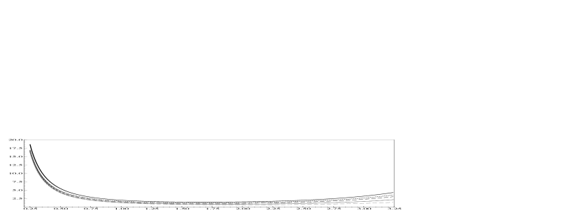
Figure 4: Theoretical results for relative computing time. $\textsc{\small{lRCT}}_{2}(\sigma)$ (solid black) is displayed together with $\textsc{\small aRCT}(\sigma,l)$ against $\sigma$. $\textsc{\small aRCT}(\sigma,l)$, the relative computing time for the limiting case of a random walk proposal, is evaluated for $l=0.5$ (dotted black), $1$ (dashed black), $2.5$ (solid grey) and $10$ (dashed grey), where $l$ is the scaling factor in the proposal.

Appendix F Simulation results

This section applies the pseudo-marginal algorithm to a linear Gaussian state-space model and presents additional simulation results for the stochastic volatility model discussed in the main paper. The linear Gaussian state-space model we consider is a first order autoregression AR$(1)$ observed with noise. In this case, $Y_{t}=X_{t}+\sigma_{\varepsilon}\varepsilon_{t}$, and the state evolution is $X_{t+1}=\mu_{x}(1-\phi)+\phi X_{t}+\sigma_{\eta}\eta_{t}$, where $\varepsilon_{t}$ and $\eta_{t}$ are standard normal and independent. We take $\phi=0.8,$ $\mu_{x}=0.5,$ $\sigma_{\eta}^{2}=1-\phi^{2}$, so that the marginal variance $\sigma_{x}^{2}$ of the state $X_{t}$ is $1$. We consider a series of length $T$, where $\sigma_{\varepsilon}^{2}=0.5$ is assumed known. The parameters of interest are therefore $\theta=(\phi,\mu_{x},\sigma_{x})$. The analysis is very similar to that of Section 4 of the main paper. However, for this state-space model, the likelihood can be calculated by using the Kalman filter. This facilitates the analysis of sections F.1 and F.2 in two ways. First, in the calculation of the log-likelihood error $Z=\log\widehat{p}_{N}(y\mid\theta)-\log p(y\mid\theta)$, the true likelihood term is known rather than estimated. Second, because the likelihood is known, we can directly examine the exact chain $Q_{\textsc{ex}}$ and estimate the inefficiency $\textsc{\small IF}(h,Q_{\textsc{ex}})$.

F.1 Empirical results for the error of the log-likelihood estimator

The analysis in this section mirrors that of Section 4.2 of the main paper. We investigate empirically Assumptions 1 and 2 by examining the behaviour of $Z=\log\widehat{p}_{N}(y\mid\theta)-\log p(y\mid\theta)$ for $T=40$, $300$ and $2700$. Corresponding values of $N$ are selected in each case to ensure that the variance of $Z$ evaluated at the posterior mean $\overline{\theta}$ is approximately unity. The three plots on the left of Fig. 5 display the histograms corresponding to the density $g_{N}(z\mid\overline{\theta})$ of $Z$ for $\theta=\overline{\theta}$, which is obtained by running $S=6000$ particle filters at this value. We overlay on each histogram a kernel density estimate together with the corresponding assumed density, $g_{\textsc{z}}^{\sigma}\left(z\right)$ of Assumption 2, where $\sigma^{2}$ is the sample variance of $Z$ over the $S$ particle filters. For $T=40$, there is a slight discrepancy between the assumed Gaussian densities and the true histograms representing $g_{N}(z\mid\overline{\theta})$. In particular, whilst $g_{N}(z\mid\overline{\theta})$ is well approximated over most of its support, it is heavier tailed in the left tail. For $T=300$ and $T=2700$, the assumed Gaussian densities are very accurate.

Figure 5: AR(1) plus noise model experiment. Top to bottom: ${T=40,}$ $N=4$ (top), $T=300,$ $N=50$ (middle), $T=2700,$ $N=500$ (bottom). Left to right: histograms and theoretical densities associated with $g_{N}(z\mid\theta)$ evaluated at the posterior mean $\overline{\theta}$ (left), over values from the posterior $\pi(\theta)$ (right). The densities $g_{\textsc{z}}^{\sigma}(z)$ are overlaid (solid lines).

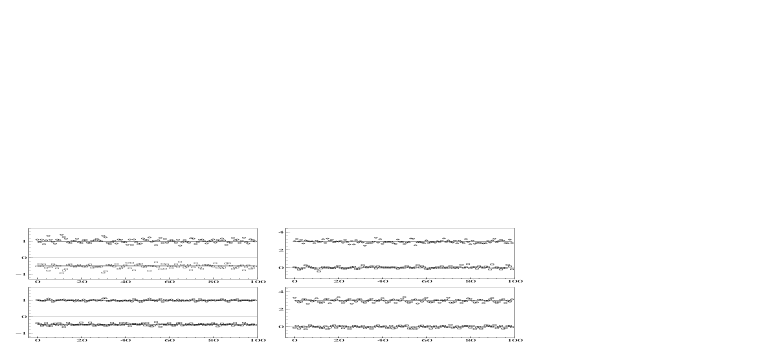
Figure 6: AR(1) plus noise model experiment. Top to bottom: $T=300,$ $N=50$ (top), $T=2700,$ $N=500$ (bottom). Left to right: mean (squares) and variance (circles) associated with $g_{N}(z\mid\theta)$ for $100$ different values of $\theta$ from $\pi(\theta)$ (left). The corresponding estimates of the third (squares) and fourth (circles) moments are displayed.

We also examine $Z$ when $\theta$ is distributed according to $\pi(\theta)$. We record $100$ samples from $\pi(\theta)$, for $T=40$, $300$ and $2700$. For each of these samples, we run the particle filter $300$ times in order to estimate the true likelihood at these values. The resulting histograms, corresponding to the density ${\textstyle\int}\pi\left(\mathrm{d}\theta\right)g_{N}(z\mid\theta)$ are displayed on the right panel of Fig. 5. For $T=300$ and $T=2700$, the assumed densities $g_{\textsc{z}}^{\sigma}\left(z\right)$ are close to the corresponding histograms and Assumptions 1 and 2 again appear to capture reasonably well the salient features of the densities associated with $Z$.

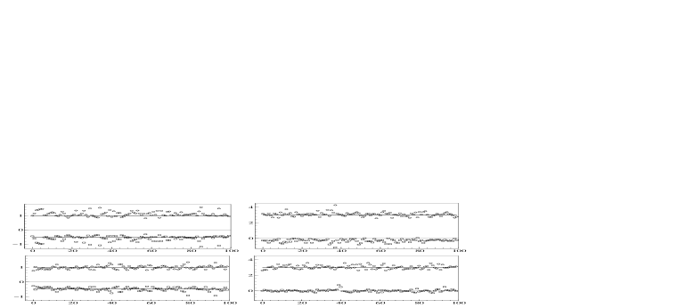
Figure 7: Huang and Tauchen two factor model experiment for S&P 500 data. Top to bottom: $T=300,$ $N=80$ (top), $T=2700,$ $N=700$ (bottom). Left to right: mean (squares) and variance (circles) associated with $g_{N}(z\mid\theta)$ for $100$ different values of $\theta$ from $\pi(\theta)$ (left). The corresponding estimates of the third (squares) and fourth (circles) moments are displayed.

It is important, in examining departures from Assumption 1, to consider the heterogeneity of the conditional density $g_{N}(z\mid\theta)$ as $\theta$ varies over $\pi\left(\theta\right)$. In Fig. 6, the conditional moments associated with the density $g_{N}(z\mid\theta)$ are estimated, based on running the particle filter independently $S=300$ times for each of $100$ values of $\theta$ from $\pi(\theta)$. We record the estimates of the mean, the variance and the third and fourth central moments at each value of $\theta$, for $T=300$ and $T=2700$. There is a small degree of variability for $T=300$ around the values that we would expect which are $-0.5,$ $1,0$ and $3$ corresponding to $g_{\textsc{z}}^{\sigma}\left(z\right)$ where $\sigma=1$. This variability reduces as $T$ rises to $2700$. A small degree variability is expected as these are moments estimated from $S=300$ samples. This lack of heterogeneity explains why the values of $Z$, marginalized over $\pi\left(\theta\right)$, on the right hand side of Fig. 5, are close to $g_{\textsc{z}}^{\sigma}\left(z\right)$ for time series of moderate and large length. Figure 7 records a similar experiment for the stochastic volatility model and data considered in Section 4 of the main paper. There is rather more variability as the true value of the likelihood in this case is unknown and has to be estimated. However, the results are similar and the variability again reduces as $T$ rises to $2700$.

F.2 Empirical results for the pseudo-marginal algorithm

The pseudo-marginal algorithm is applied to $T=300$ data. The true likelihood of the data is computed by the Kalman filter as the model is a linear Gaussian state space model. This allows the exact Metropolis–Hastings scheme $Q_{\textsc{ex}}$ to be implemented so that the corresponding inefficiency $\textsc{\small IF}\left(h,Q_{\textsc{ex}}\right)$ can be easily estimated. We consider varying $N$ so that the standard deviation $\sigma(\overline{\theta};N)$ of the log-likelihood estimator varies. The grid of values that we consider for $N$ is $\{11$, $16$, $22$, $31$, $43$, $60$, $83$, $116$, $161$, $224$, $312\}$, see Table 2. The value $N=60$ results in $\sigma(\overline{\theta};N)=0.92$.

Table 2: AR(1) plus noise example with proposal parameter $\rho=0,T=300,\phi=0.8,\mu=0.5,\sigma_{x}^{2}=1$ and $\sigma_{\varepsilon}^{2}=0.5$. Inefficiencies $(\textsc{{\small IF}})$ and computing times $(\textsc{{\small CT=$N$ $\times$ IF}})$ shown for $(\phi,\mu,\sigma_{x})$ and marginal probabilities of acceptance. See Fig. 8 and Fig. 9.

$Q_{\textsc{ex}}$		IF$(\phi)$	IF$(\mu)$	IF$(\sigma_{x})$				pr$(Acc)$
		$2.5845$	$2.5040$	$2.4163$				$0.7678$
$Q$
$N$	$\sigma(\overline{\theta};N)$	IF$(\phi)$	IF$(\mu)$	IF$(\sigma_{x})$	CT$(\phi)$	CT$(\mu)$	CT$(\sigma_{x})$	pr$(Acc)$
$11$	$2.2886$	$136.32$	$132.41$	$128.66$	$1499.5$	$1456.5$	$1415.3$	$0.11424$
$16$	$1.8692$	$61.403$	$63.756$	$66.609$	$982.45$	$1020.1$	$1065.7$	$0.19036$
$22$	$1.6063$	$37.256$	$40.486$	$37.367$	$819.63$	$890.68$	$822.07$	$0.25549$
$31$	$1.3412$	$15.880$	$18.099$	$19.135$	$492.29$	$561.08$	$593.20$	$0.32622$
$43$	$1.1096$	$11.320$	$9.7400$	$10.710$	$486.75$	$418.82$	$460.54$	$0.39347$
$60$	$0.9197$	$7.5040$	$8.0428$	$7.6168$	$450.24$	$482.57$	$457.01$	$0.45933$
$83$	$0.8058$	$5.7253$	$5.5841$	$5.9348$	$475.20$	$463.48$	$492.59$	$0.50885$
$116$	$0.6828$	$4.3756$	$4.7106$	$4.1693$	$507.57$	$546.43$	$483.63$	$0.56621$
$161$	$0.5828$	$3.8112$	$4.2379$	$3.6388$	$613.61$	$682.30$	$585.84$	$0.60160$
$224$	$0.4838$	$3.2711$	$3.1605$	$3.3134$	$732.73$	$707.94$	$742.19$	$0.63562$
$312$	$0.4096$	$3.0774$	$3.4768$	$2.8355$	$960.14$	$1084.8$	$884.67$	$0.65793$

Table 3: AR(1) plus noise example with proposal parameter $\rho=0.9$. Other settings identical to Table 2.

$Q_{\textsc{ex}}$		IF$(\phi)$	IF$(\mu)$	IF$(\sigma_{x})$				pr$(Acc)$
		$25.59$	$22.21$	$24.44$				$0.87717$
$Q$
$N$	$\sigma(\overline{\theta};N)$	IF$(\phi)$	IF$(\mu)$	IF$(\sigma_{x})$	CT$(\phi)$	CT$(\mu)$	CT$(\sigma_{x})$	pr$(Acc)$
$11$	$2.2886$	$594.64$	$488.30$	$639.04$	$6541.1$	$5371.3$	$7029.5$	$0.12579$
$16$	$1.8692$	$157.49$	$183.78$	$182.07$	$2519.9$	$2940.4$	$2913.1$	$0.20410$
$22$	$1.6063$	$126.87$	$115.84$	$125.37$	$2791.2$	$2548.6$	$2758.2$	$0.27279$
$31$	$1.3412$	$69.541$	$67.421$	$71.982$	$2155.9$	$2089.9$	$2231.5$	$0.35385$
$43$	$1.1096$	$53.053$	$62.344$	$58.002$	$2281.1$	$2680.9$	$2494.0$	$0.42577$
$60$	$0.9197$	$49.351$	$47.476$	$45.194$	$2961.1$	$2848.6$	$2711.6$	$0.49610$
$83$	$0.8058$	$37.709$	$29.550$	$38.266$	$3129.8$	$2452.7$	$3176.1$	$0.55764$
$116$	$0.6828$	$29.360$	$36.943$	$34.892$	$3405.8$	$4285.4$	$4047.4$	$0.61174$
$161$	$0.5828$	$28.277$	$27.883$	$29.864$	$4552.6$	$4489.2$	$4808.1$	$0.65704$
$224$	$0.4838$	$27.770$	$29.471$	$30.533$	$6220.5$	$6601.5$	$6839.4$	$0.69674$
$312$	$0.4096$	$29.231$	$25.549$	$29.967$	$9120.2$	$7971.4$	$9349.8$	$0.73057$

We transform each of the parameters to the real line so that $\Psi=k(\theta)$, where both $\theta$ and $\Psi$ are three dimensional vectors, and place a Gaussian prior on $\Psi$ centred at zero with a large variance. We use the autoregressive Metropolis proposal $q(\Psi,\Psi^{\ast})$

$$\Psi^{\ast}=(1-\rho)\widehat{\Psi}+\rho\Psi+(1-\rho^{2})^{1/2}\{(\nu-2)/\nu\}^{1/2}\Sigma^{1/2}t_{\nu},$$

for both the pseudo-marginal algorithm and exact likelihood schemes, where $\widehat{\Psi}$ is the mode of the log-likelihood obtained from the Kalman filter and the covariance $\Sigma$ is the negative inverse of the second derivative of the log-likelihood at the mode.  Here $t_{\nu}$ denotes a standard multivariate t-distributed random variable with $\nu$ degrees of freedom. We set $\nu=5$. We use this autoregressive proposal with the scalar autoregressive parameter $\rho$ chosen as one of $\{0$, $0.4$, $0.6$, $0.9\}$. We first apply this proposal, for the four values of $\rho$, using the known likelihood in the Metropolis scheme and estimate the inefficiency for each of the parameters $\theta=(\mu_{x},\phi,\sigma_{\eta})$.

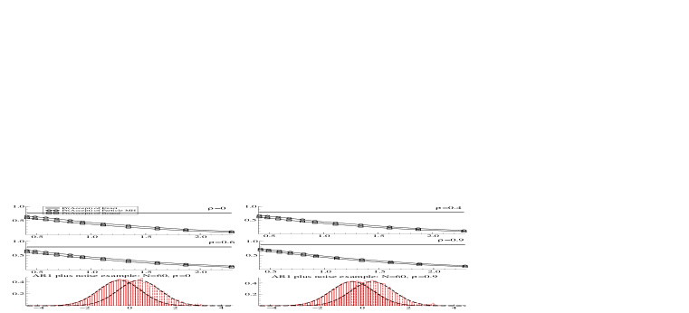
Figure 8: AR(1) plus noise example with $T=300,\phi=0.8,\mu=0.5,\sigma_{x}^{2}=1,\sigma_{\varepsilon}^{2}$ fixed at $0.5$. Marginal acceptance probabilities displayed against $\sigma(\overline{\theta};N)$. The estimated (constant) marginal probabilities of acceptance for $Q_{\textsc{ex}}$ are shown (solid line) together with the estimated probabilities (circles) from $Q$. The lower bound (squares) is given as the probability from the exact scheme times $2\Phi(-\sigma/\surd{2})$. The proposal autocorrelations are $\rho=0,0.4,0.6$ and $0.9$. See Tables 2 and 3. Bottom: Histograms for the accepted and proposed values of $Z$, the log-likelihood error for $\rho=0$ (left) and for $\rho=0.9$ (right). The theoretical Gaussian densities for the proposal $\varphi(-\sigma^{2}/2,\sigma^{2})$ and the accepted values $\varphi(\sigma^{2}/2,\sigma^{2})$ are overlaid where $\sigma=\sigma(\overline{\theta};N)$.

Figure 9: AR(1) plus noise example with $T=300,$ $\phi=0.8,\mu=0.5,$ $\sigma_{x}^{2}=1$ and $\sigma_{\varepsilon}^{2}$ fixed at $0.5$. Left: Logarithm rif against $\sigma(\overline{\theta};N)$. Right: rct $=\textsc{rif}/\sigma^{2}(\overline{\theta};N)$ against $\sigma(\overline{\theta};N)$. The three plots on all graphs are for $\phi$ (square), $\mu$ (circle) and $\sigma_{x}$ (cross). From Top to bottom: $\rho=0,$ $0.4,0.6$ and $0.9$. Here $\sigma(\overline{\theta};N)$ is the standard deviation of the log-likelihood estimator evaluated at the posterior mean $\overline{\theta}$. See Tables 2 and 3.

Figure 8 shows the acceptance probability for the pseudo-marginal algorithm against $\sigma(\overline{\theta};N)$ for the four values of the proposal parameter $\rho$. The lower bound for the acceptance probabilities, as discussed at the end of Section 4.3 of the main paper, is also displayed and there is close correspondence in all cases. The histograms for the accepted and rejected values of $Z$, for $N=60$ when $\sigma(\overline{\theta};N)=0.92$, are also displayed. The approximating asymptotic Gaussian densities, with $\sigma=0.92$, are superimposed. This figure shows that the approximating densities correspond very closely to the two histograms. It should be noted that these are the marginal values for $Z$ over the draws from the posterior $\pi(\theta)$ obtained by running the pseudo-marginal scheme, rather than being based upon a fixed value of the parameters.

Tables 2 and 3 show the pseudo-marginal algorithm results for $\rho=0$ and $\rho=0.9$. For the independent Metropolis–Hastings proposal, it is clear from Table 2, that the computing time in minimised around $N=43$ or $60$, depending on which parameter is examined, with the corresponding values of $\sigma(\overline{\theta};N)$ being $1.11$ and $0.92$, supporting the findings that when an efficient proposal is used the optimal value of $\sigma$ is close to unity. This is again supported by Fig. 9, for which the relative computing time ($\rho=0$ is the top right plot) is shown against $\sigma(\overline{\theta};N)$. We note that the relative inefficiencies and computing times are straightforward to calculate as the exact chain inefficiencies for the three parameters have been calculated and are given in the top row of Table 2. Table 3 shows the results for the more persistent proposal where $\rho=0.9$. In this case, for all three parameters the optimal value of $N$ is around $31$, at which $\sigma(\overline{\theta};N)=1.34$, the corresponding graph of the relative computing time being given by the bottom right of Fig. 9. It is clear that again the findings are consistent with the discussion of 3.5 in the main paper. In particular, as $\rho$ increases, then $\textsc{\small IF}\left(h,Q^{\textsc{ex}}\right)$ should increase, and, from Fig. 9, it is clear that the optimal value of $\sigma(\overline{\theta};N)$ increases, the relative computing time decreases for any given $\sigma(\overline{\theta};N)$. In addition, the relative computing time becomes more flat as a function of $\sigma(\overline{\theta};N)$ as $\rho$ increases.

Appendix G Numerical procedures

Under the Gaussian assumption, Corollary 3 specifies the function $\varrho_{\textsc{z}}^{\sigma}$ and the term $\pi_{\textsc{z}}^{\sigma}\left(1/\varrho_{\textsc{z}}^{\sigma}\right)$ can be accurately evaluated using numerical quadrature. This section explains how we numerically evaluate the terms $\phi_{\textsc{z}}^{\sigma}$ and $\textsc{\small IF}(1/\varrho_{\textsc{z}}^{\sigma},{\widetilde{Q}^{\textsc{z}}})$ which appear in the bounds of Corollaries 1 and 2. The inefficiency $\textsc{\small IF}(1/\varrho_{\textsc{z}}^{\sigma},{\widetilde{Q}^{\textsc{z}}})$ is finite by Lemma 3, because $\pi_{\textsc{z}}^{\sigma}\left(1/\varrho_{\textsc{z}}^{\sigma}\right)$ is finite. The autocorrelations quickly descend to zero as a function of $n$, for all $\sigma$. Hence, it is straightforward to estimate $\textsc{\small IF}(1/\varrho_{\textsc{z}}^{\sigma},{\widetilde{Q}^{\textsc{z}}})$ by the appropriate summation of the autocorrelations, and to tabulate it against $\sigma$ for use in the bounds of Corollaries 1 and 2. The autocorrelation $\phi_{\textsc{z}}^{\sigma}$, for $n=1$, is similarly tabulated.

From Lemma 3,

$$\widetilde{Q}^{\textsc{z}}\left(z,\mathrm{d}w\right)=\frac{g\left(w\right)\min\{1,\exp(w-z)\}\mathrm{d}w}{\varrho_{\textsc{z}}\left(z\right)},\text{ \ }\widetilde{\pi}_{\textsc{z}}\left(\mathrm{d}z\right)=\frac{\pi_{\textsc{z}}\left(\mathrm{d}z\right)\varrho_{\textsc{z}}\left(z\right)}{\pi_{\textsc{z}}\left(\varrho_{\textsc{z}}\right)},$$

so the autocorrelation at lag $n$ is

$$\phi_{n}\left(\varrho_{\textsc{z}}^{-1},\widetilde{Q}^{\textsc{z}}\right)=\frac{\left\langle\varrho_{\textsc{z}}^{-1},\left(\widetilde{Q}^{\textsc{z}}\right)^{n}\varrho_{\textsc{z}}^{-1}\right\rangle_{\widetilde{\pi}_{\textsc{z}}}{-}\left\{\widetilde{\pi}_{\textsc{z}}\left(\varrho_{\textsc{z}}^{-1}\right)\right\}^{2}}{\mathbb{V}_{\widetilde{\pi}_{Z}}\left(\varrho_{\textsc{z}}^{-1}\right)}$$

with

$$\left\langle\varrho_{\textsc{z}}^{-1},\left(\widetilde{Q}^{\textsc{z}}\right)^{n}\varrho_{\textsc{z}}^{-1}\right\rangle_{\widetilde{\pi}_{\textsc{z}}} ={\textstyle\int}\varrho_{\textsc{z}}^{-1}(z_{0})\varrho_{\textsc{z}}^{-1}(z_{n})\widetilde{\pi}_{\textsc{z}}(\mathrm{d}z_{0})\left(\widetilde{Q}^{\textsc{z}}\right)^{n}\left(z_{0},\mathrm{d}z_{n}\right)$$

$$=\pi_{\textsc{z}}(\varrho_{\textsc{z}})^{-1}{\textstyle\int}\varrho_{\textsc{z}}^{-1}(z_{n})\widetilde{\pi}_{\textsc{z}}(\mathrm{d}z_{0})\left(\widetilde{Q}^{\textsc{z}}\right)^{n}\left(z_{0},\mathrm{d}z_{n}\right).$$ (50)

The term $\pi_{\textsc{z}}(\varrho_{\textsc{z}})$ can be computed by quadrature. The term (50) can be also accurately calculated by Monte Carlo integration, by simulating a large number $M$ of i.i.d. samples $Z_{0}^{i}\sim\pi_{\textsc{z}}$ and then propagating each sample through the transition kernel ${\widetilde{Q}^{\textsc{z}}}$ $n$ times to obtain $Z_{n}^{i}\sim\pi_{\textsc{z}}(\widetilde{Q}^{\textsc{z}})^{n}$, yielding the estimate $\frac{1}{M}\sum_{i=1}^{M}\varrho_{\textsc{z}}^{-1}(Z_{n}^{i}).$

References

- Andrieu et al. (2010) Andrieu, C., Doucet, A. & Holenstein, R. (2010). Particle Markov chain Monte Carlo methods. Journal of the Royal Statistical Society, Series B 72, 1–33.
- Andrieu & Vihola (2014) Andrieu, C. & Vihola, M. (2014). Establishing some order amongst exact approximations of MCMCs, arXiv:1404.6909.
- Andrieu & Vihola (2012) Andrieu, C. & Vihola, M. (2012). Convergence properties of pseudo-marginal Markov Chain Monte Carlo algorithms. Annals of Applied Probability, to appear.
- Andrieu & Roberts (2009) Andrieu, C. & Roberts, G. O. (2009). The pseudo-marginal approach for efficient Monte Carlo computations. The Annals of Statistics 37, 697–725.
- Baxendale (2005) Baxendale, P. (2005). Renewal theory and computable convergence rates for geometrically ergodic Markov chains. The Annals of Applied Probability 15, 700–738.
- Beaumont (2003) Beaumont, M. (2003a). Estimation of population growth or decline in genetically monitored populations. Genetics 164, 1139.
- Chernov et al. (2003) Chernov, M., Gallant, A. R., Ghysels, E. & Tauchen, G. (2003). Alternative models of stock price dynamics. Journal of Econometrics 116, 225–257.
- Douc & Robert (2011) Douc, R. & Robert, C. P. (2011). A vanilla Rao–Blackwellization of Metropolis–Hastings algorithms. The Annals of Statistics 39, 261–277.
- Geyer (1992) Geyer, C. J. (1992). Practical Markov chain Monte Carlo. Statistical Science 7, 473–483.
- Häggström & Rosenthal (2007) Häggström, O. & Rosenthal, J. S. (2007). On variance conditions for Markov chain central limit theorems. Electronic Communications in Probability 12, 454–64.
- Huang & Tauchen (2005) Huang, X. & Tauchen, G. (2005). The relative contribution of jumps to total price variation. Journal of Financial Econometrics 3, 456–499.
- Lin et al. (2000) Lin, L., Liu, K. F. & Sloan, J. (2000). A noisy Monte Carlo algorithm. Physical Review D 61, 074505.
- Peskun (1973) Peskun, P. H. (1973). Optimum Monte–Carlo sampling using Markov chains. Biometrika 60, 607–612.
- Pitt et al. (2012) Pitt, M. K., Silva, R., Giordani, P. & Kohn, R. (2012). On some properties of Markov chain Monte Carlo simulation methods based on the particle filter. Journal of Econometrics 171, 134–151.
- Roberts & Tweedie (1996) Roberts, G. & Tweedie, R. (1996). Geometric convergence and central limit theorems for multidimensional Hastings and Metropolis algorithms. Biometrika 83, 95–110.
- Rudolf & Ullrich (2013) Rudolf, D. & Ullrich, M. (2013). Positivity of hit-and-run and related algorithms. Electronic Communications in Probability 18, 1–8.
- Tierney (1994) Tierney, L. (1994). Markov chains for exploring posterior distributions (with discussion). The Annals of Statistics 21, 1701–62.
- Tierney (1998) Tierney, L. (1998). A note on Metropolis–Hastings kernels for general state spaces. The Annals of Applied Probability 8, 1–9.
- Kipnis & Varadhan (1986) Kipnis, C. & Varadhan, S. (1986). Central limit theorem for additive functionals of reversible Markov processes and applications to simple exclusions. Communications in Mathematical Physics 104, 1–19.
- Meyn & Tweedie (2009) Meyn, S. & Tweedie, R.L. (1991). Markov Chains and Stochastic Stability. Second edition. Cambridge University Press, Cambridge.
- Rudin (1991) Rudin, W. (1991). Functional Analysis. International series in pure and applied mathematics. McGraw-Hill, Inc., New York.
- Sherlock et al. (2013) Sherlock, C., Thiery, A., Roberts, G. & Rosenthal, J. (2013). On the efficiency of pseudo-marginal random walk Metropolis algorithms. ArXiv e-prints URL: http://arxiv.org/abs/1309.7209.
- Schmüdgen (2012) Schmüdgen, K. (2012). Unbounded Self-adjoint Operators on Hilbert Space. Graduate Text in Mathematics, Springer.
- Wu & Woodroofe (2004) Wu, W. & Woodroofe, M. (2004). Martingale approximations for sums of stationary processes. The Annals of Probability 32, 1674–1690.