Constraints on the Universe as a Numerical Simulation

Abstract

Observable consequences of the hypothesis that the observed universe is a numerical simulation performed on a cubic space-time lattice or grid are explored. The simulation scenario is first motivated by extrapolating current trends in computational resource requirements for lattice QCD into the future. Using the historical development of lattice gauge theory technology as a guide, we assume that our universe is an early numerical simulation with unimproved Wilson fermion discretization and investigate potentially-observable consequences. Among the observables that are considered are the muon $g-2$ and the current differences between determinations of $\alpha$, but the most stringent bound on the inverse lattice spacing of the universe, $b^{-1}\raisebox{-3.01385pt}{$\stackrel{{\scriptstyle\textstyle>}}{{\sim}}$ }10^{11}~{}{\rm GeV}$, is derived from the high-energy cut off of the cosmic ray spectrum. The numerical simulation scenario could reveal itself in the distributions of the highest energy cosmic rays exhibiting a degree of rotational symmetry breaking that reflects the structure of the underlying lattice.

I Introduction

Extrapolations to the distant futurity of trends in the growth of high-performance computing (HPC) have led philosophers to question —in a logically compelling way— whether the universe that we currently inhabit is a numerical simulation performed by our distant descendants Bostrom (2003). With the current developments in HPC and in algorithms it is now possible to simulate Quantum Chromodynamics (QCD), the fundamental force in nature that gives rise to the strong nuclear force among protons and neutrons, and to nuclei and their interactions. These simulations are currently performed in femto-sized universes where the space-time continuum is replaced by a lattice, whose spatial and temporal sizes are of the order of several femto-meters or fermis ($1~{}{\rm fm}=10^{-15}~{}{\rm m}$), and whose lattice spacings (discretization or pixelation) are fractions of fermis . This endeavor, generically referred to as lattice gauge theory, or more specifically lattice QCD, is currently leading to new insights into the nature of matter . Within the next decade, with the anticipated deployment of exascale computing resources, it is expected that the nuclear forces will be determined from QCD, refining and extending their current determinations from experiment, enabling predictions for processes in extreme environments, or of exotic forms of matter, not accessible to laboratory experiments. Given the significant resources invested in determining the quantum fluctuations of the fundamental fields which permeate our universe, and in calculating nuclei from first principles (for recent works, see Refs. Beane et al. (2012); Yamazaki et al. (2012); Aoki et al. (2012)), it stands to reason that future simulation efforts will continue to extend to ever-smaller pixelations and ever-larger volumes of space-time, from the femto-scale to the atomic scale, and ultimately to macroscopic scales. If there are sufficient HPC resources available, then future scientists will likely make the effort to perform complete simulations of molecules, cells, humans and even beyond. Therefore, there is a sense in which lattice QCD may be viewed as the nascent science of universe simulation, and, as will be argued in the next paragraph, very basic extrapolation of current lattice QCD resource trends into the future suggest that experimental searches for evidence that our universe is, in fact, a simulation are both interesting and logical.

There is an extensive literature which explores various aspects of our universe as a simulation, from philosophical discussions Bostrom (2003), to considerations of the limits of computation within our own universe Lloyd (1999), to the inclusion of gravity and the standard model of particle physics into a quantum computation Lloyd (2005), and to the notion of our universe as a cellular automaton Zuse (1969); Fredkin (1990); Wolfram (2002); ’t Hooft (2012). There have also been extensive connections made between fundamental aspects of computation and physics, for example, the translation of the Church-Turing principle Church (1936); Turing (1936) into the language of physicists by Deutsch Deutsch (1985). Finally, the observational consequences due to limitations in accuracy or flaws in a simulation have been considered Barrow (2008). In this work, we take a pedestrian approach to the possibility that our universe is a simulation, by assuming that a classical computer (i.e. the classical limit of a quantum computer) is used to simulate the quantum universe (and its classical limit), as is done today on a very small scale, and ask if there are any signatures of this scenario that might be experimentally detectable. Further, we do not consider the implications of, and constraints upon, the underlying information, and its movement, that are required to perform such extensive simulations. It is the case that the method of simulation, the algorithms, and the hardware that are used in future simulations are unknown, but it is conceivable that some of the ingredients used in present day simulations of quantum fields remain in use, or are used in other universes, and so we focus on one aspect only: the possibility that the simulations of the future employ an underlying cubic lattice structure.

In contrast with Moore’s law, which is a statement about the exponential growth of raw computing power in time, it is interesting to consider the historical growth of measures of the computational resource requirements (CRRs) of lattice QCD calculations, and extrapolations of this trend to the future. In order to do so, we consider two lattice generation programs: the MILC asqtad program MILC-Collaboration , which over a twelve year span generated ensembles of lattice QCD gauge configurations, using the Kogut-Susskind Kogut and Susskind (1975) (staggered) discretization of the quark fields, with lattice spacings, $b$, ranging from $0.18$ to $0.045~{}$fm, and lattice sizes (spatial extents), $L$, ranging from $2.5$ to $5.8~{}$fm, and the on-going anisotropic program carried out by the SPECTRUM collaboration SPECTRUM-Collaboration , using the clover-Wilson Wilson (1974); Sheikholeslami and Wohlert (1985) discretization of the quark fields, which has generated lattice ensembles at $b\sim 0.1~{}$fm, with $L$ ranging from $2.4$ to $4.9~{}$fm Lin et al. (2009). At fixed quark masses, the CRR of a lattice ensemble generation (in units of petaFLOP-years) scales roughly as the dimensionless number $\lambda_{QCD}L^{5}/b^{6}$, where $\lambda_{QCD}\equiv 1~{}$fm is a typical QCD distance scale. In fig. 1 (left panel), the CRRs are presented on a logarithmic scale, where year one corresponds to 1999, when MILC initiated its asqtad program of $2+1$-flavor ensemble generation. The bands are linear fits to the data. While the CRR curves in some sense track Moore’s law, they are more than a statement about increasing FLOPS. Since lattice QCD simulations include the quantum fluctuations of the vacuum and the effects of the strong nuclear force, the CRR curve is a statement about simulating universes with realistic fundamental forces. The extrapolations of the CRR trends into the future are shown in the right panel of fig. 1.

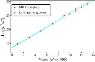
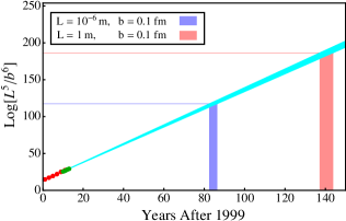
Figure 1: Left panel: linear fit to the logarithm of the CRRs of MILC asqtad and the SPECTRUM anisotropic lattice ensemble generations. Right panel: extrapolation of the fit curves into the future, as discussed in the text. The blue (red) horizontal line corresponds to lattice sizes of one micron (meter), and vertical bands show the corresponding extrapolated years beyond 1999 for the lattice generation programs.

The blue (red) horizontal line corresponds to a lattice of the size of a micro-meter (meter), a typical length scale of a cell (human), and at a lattice spacing of $0.1~{}$fm. There are, of course, many caveats to this extrapolation. Foremost among them is the assumption that an effective Moore’s Law will continue into the future, which requires technological and algorithmic developments to continue as they have for the past 40 years. Related to this is the possible existence of the technological singularity Vinge (1993); Kurzweil (2006), which could alter the curve in unpredictable ways. And, of course, human extinction would terminate the exponential growth Bostrom (2003). However, barring such discontinuities in the curve, these estimates are likely to be conservative as they correspond to full simulations with the fundamental forces of nature. With finite resources at their disposal, our descendants will likely make use of effective theory methods, as is done today, to simulate every-increasing complexity, by, for instance, using meshes that adapt to the relevant physical length scales, or by using fluid dynamics to determine the behavior of fluids, which are constrained to rigorously reproduce the fundamental laws of nature. Nevertheless, one should keep in mind that the CRR curve is based on lattice QCD ensemble generation and therefore is indicative of the ability to simulate the quantum fluctuations associated with the fundamental forces of nature at a given lattice spacing and size. The cost to perform the measurements that would have to be done in the background of these fluctuations in order to simulate —for instance— a cell could, in principle, lie on a significantly steeper curve.

We should comment on the simulation scenario in the context of ongoing attempts to discover the theoretical structure that underlies the Standard Model of particle physics, and the expectation of the unification of the forces of nature at very short distances. There has not been much interest in the notion of an underlying lattice structure of space-time for several reasons. Primary among them is that in Minkowski space, a non-vanishing spatial lattice spacing generically breaks space-time symmetries in such a way that there are dimension-four Lorentz breaking operators in the Standard Model, requiring a large number of fine-tunings to restore Lorentz invariance to experimentally verified levels Coleman and Glashow (1999). The fear is that even though Lorentz violating dimension four operators can be tuned away at tree-level, radiative corrections will induce them back at the quantum level as is discussed in Refs. Gagnon and Moore (2004); Collins et al. (2004). This is not an issue if one assumes the simulation scenario for the same reason that it is not an issue when one performs a lattice QCD calculation . The underlying space-time symmetries respected by the lattice action will necessarily be preserved at the quantum level. In addition, the notion of a simulated universe is sharply at odds with the reductionist prejudice in particle physics which suggests the unification of forces with a simple and beautiful predictive mathematical description at very short distances. However, the discovery of the string landscape Kachru et al. (2003); Susskind (2003), and the current inability of string theory to provide a useful predictive framework which would post-dict the fundamental parameters of the Standard Model, provides the simulators (future string theorists?) with a purpose: to systematically explore the landscape of vacua through numerical simulation. If it is indeed the case that the fundamental equations of nature allow on the order of $10^{500}$ solutions Douglas (2003), then perhaps the most profound quest that can be undertaken by a sentient being is the exploration of the landscape through universe simulation. In some weak sense, this exploration is already underway with current investigations of a class of confining beyond-the-Standard-Model (BSM) theories, where there is only minimal experimental guidance at present (for one recent example, see Ref. Appelquist et al. (2012)). Finally, one may be tempted to view lattice gauge theory as a primitive numerical tool, and that the simulator should be expected to have more efficient ways of simulating reality. However, one should keep in mind that the only known way to define QCD as a consistent quantum field theory is in the context of lattice QCD, which suggests a fundamental role for the lattice formulation of gauge theory.

Physicists, in contrast with philosophers, are interested in determining observable consequences of the hypothesis that we are a simulation  . In lattice QCD, space-time is replaced by a finite hyper-cubic grid of points over which the fields are defined, and the (now) finite-dimensional quantum mechanical path integral is evaluated. The grid breaks Lorentz symmetry (and hence rotational symmetry), and its effects have been defined within the context of a low-energy effective field theory (EFT), the Symanzik action, when the lattice spacing is small compared with any physical length scales in the problem Symanzik (1983, 1983) . The lattice action can be modified to systematically improve calculations of observables, by adding irrelevant operators with coefficients that can be determined nonperturbatively. For instance, the Wilson action can be ${\cal O}(b)$-improved by including the Sheikholeslami-Wohlert term Sheikholeslami and Wohlert (1985). Given this low-energy description, we would like to investigate the hypothesis that we are a simulation with the assumption that the development of simulations of the universe in some sense parallels the development of lattice QCD calculations. That is, early simulations use the computationally “cheapest” discretizations with no improvement. In particular, we will assume that the simulation of our universe is done on a hyper-cubic grid  and, as a starting point, we will assume that the simulator is using an unimproved Wilson action, that produces ${\cal O}(b)$ artifacts of the form of the Sheikholeslami-Wohlert operator in the low-energy theory .

In section II, the simple scenario of an unimproved Wilson action is introduced. In section III, by looking at the rotationally-invariant dimension-five operator arising from this action, the bounds on the lattice spacing are extracted from the current experimental determinations, and theoretical calculations, of $g-2$ of the electron and muon, and from the fine-structure constant, $\alpha$, determined by the Rydberg constant. Section IV considers the simplest effects of Lorentz symmetry breaking operators that first appear at ${\cal O}(b^{2})$, and modifications to the energy-momentum relation. Constraints on the energy-momentum relation due to cosmic ray events are found to provide the most stringent bound on $b$. We conclude in section V.

II Unimproved Wilson Simulation of the Universe

The simplest gauge invariant action of fermions which does not contain doublers is the Wilson action,

$$S^{(W)} = b^{4}\sum_{x}{\cal L}^{(W)}(x)=b^{4}\left(m+{4\over b}\right)\ \sum_{x}\ \overline{\psi}(x)\psi(x)$$ (1)

$$+ {b^{3}\over 2}\sum_{x}\ \overline{\psi}(x)\left[\,\left(\gamma_{\mu}-1\right)\ U_{\mu}(x)\ \psi(x+b\hat{\mu})-\left(\gamma_{\mu}+1\right)\ U^{\dagger}_{\mu}(x-b\hat{\mu})\ \psi(x-b\hat{\mu})\,\right],$$

which describes a fermion, $\psi$, of mass $m$ interacting with a gauge field, $A_{\mu}(x)$, through the gauge link,

$$U_{\mu}(x) = \exp\ \left(ig\int_{x}^{x+b\hat{\mu}}\ dzA_{\mu}(z)\ \right),$$ (2)

where $\hat{\mu}$ is a unit vector in the $\mu$-direction, and $g$ is the coupling constant of the theory. Expanding the Lagrangian density, ${\cal L}^{(W)}$, in the lattice spacing (that is small compared with the physical length scales), and performing a field redefinition Lüscher and Weisz (1985), it can be shown that the Lagrangian density takes the form

$${\cal L}^{(W)} = \overline{\psi}D\hskip-6.49994pt/\psi\ +\ \tilde{m}\overline{\psi}\psi\ \ +\ {\cal C}_{p}{gb\over 4}\overline{\psi}\sigma_{\mu\nu}G^{\mu\nu}\psi\ +\ {\cal O}(b^{2}),$$ (3)

where $G_{\mu\nu}=-i[\,D_{\mu}\,,\,D_{\nu}\,]/g$ is the field strength tensor and $D_{\mu}$ is the covariant derivative. $\tilde{m}$ is a redefined mass which contains ${\cal O}(b)$ lattice spacing artifacts (that can be tuned away). The coefficient of the Pauli term $\overline{\psi}\sigma_{\mu\nu}G^{\mu\nu}\psi$ is fixed at tree level, ${\cal C}_{p}=1+{\cal O}(\alpha)$, where $\alpha=g^{2}/(4\pi)$. It is worth noting that as is usual in lattice QCD calculations, the lattice action can be ${\cal O}(b)$ improved by adding a term of the form $\delta{\cal L}^{(W)}=C_{sw}{gb\over 4}\overline{\psi}\sigma_{\mu\nu}G^{\mu\nu}\psi$ to the Lagrangian with $C_{sw}=-{\cal C}_{p}+{\cal O}(\alpha)$. This is the so-called Sheikholeslami-Wohlert term. Of course there is no reason to assume that the simulator had to have performed such an improvement in simulating the universe.

III Rotationally Invariant Modifications

Lorentz symmetry is recovered in lattice calculations as the lattice spacing vanishes when compared with the scales of the system. It is useful to consider contributions to observables from a non-zero lattice spacing that are Lorentz invariant and consequently rotationally invariant, and those that are not. While the former type of modifications could arise from many different BSM scenarios, the latter, particularly modifications that exhibit cubic symmetry, would be suggestive of a structure consistent with an underlying discretization of space-time.

III.0.1 QED Fine Structure Constant and the Anomalous Magnetic Moment

For our present purposes, we will assume that Quantum Electrodynamics (QED) is simulated with this unimproved action, eq. (1). The ${\cal O}(b)$ contribution to the lattice action induces an additional contribution to the fermion magnetic moments. Specifically, the Lagrange density that describes electromagnetic interactions is given by eq. (3), where the interaction with an external magnetic field $\mathbf{B}$ is described through the covariant derivative $D_{\mu}=\partial_{\mu}+ie{\hat{Q}}A_{\mu}$ with $e>0$ and the electromagnetic charge operator ${\hat{Q}}$, and where the vector potential satisfies $\nabla\times\mathbf{A}=\mathbf{B}$. The interaction Hamiltonian density in Minkowski-space is given by

$${\cal H}_{int} = {e\over 2m}\overline{\psi}A_{\mu}(i\overrightarrow{\partial}^{\mu}-i\overleftarrow{\partial}^{\mu}){\hat{Q}}\psi\ +\ {{\hat{Q}}e\over 4m}\overline{\psi}\sigma_{\mu\nu}F^{\mu\nu}\psi\ +\ {\cal C}_{p}{{\hat{Q}}eb\over 4}\overline{\psi}\sigma_{\mu\nu}F^{\mu\nu}\psi\ +\ ...\ .$$ (4)

where $F_{\mu\nu}=\partial_{\mu}A_{\nu}-\partial_{\nu}A_{\mu}$ is the electromagnetic field strength tensor, and the ellipses denote terms suppressed by additional powers of $b$. By performing a non-relativistic reduction, the last two terms in eq. 4 give rise to $\mathcal{H}_{int,mag}=-{\bm{\mu}}\cdot{\bm{B}}$, where the electron magnetic moment $\bm{\mu}$ is given by

$${\bm{\mu}} = {{\hat{Q}}e\over 2m}\left(g+2mb\ {\cal C}_{p}+...\right)\ {\bm{S}}\ =\ g(b)\ {{\hat{Q}}e\over 2m}\ {\bm{S}}\ ,$$ (5)

where $g$ is the usual fermion g-factor and ${\bm{S}}$ is its spin. Note that the lattice spacing contribution to the magnetic moment is enhanced relative to the Dirac contribution by one power of the particle mass.

For the electron, the effective $g$-factor has an expansion at finite lattice spacing of

$$\frac{g^{(e)}(b)}{2} = 1+C_{2}\left({\alpha\over\pi}\right)+C_{4}\left({\alpha\over\pi}\right)^{2}+C_{6}\left({\alpha\over\pi}\right)^{3}+C_{8}\left({\alpha\over\pi}\right)^{4}+C_{10}\left({\alpha\over\pi}\right)^{5}$$ (6)

$$\ +\ a_{\rm hadrons}\ +\ a_{\mu,\tau}\ +\ a_{\rm weak}\ +\ m_{e}b\ {\cal C}_{p}\ +\ ...\ \ \ ,$$

where the coefficients $C_{i}$, in general, depend upon the ratio of lepton masses. The calculation by Schwinger provides the leading coefficient of $C_{2}={1\over 2}$. The experimental value of $g^{(e)}_{\rm expt}/2=1.001\ 159\ 652\ 180\ 73(28)$ gives rise to the best determination of the fine structure constant $\alpha$ (at $b=0$) Mohr et al. (2012). However, when the lattice spacing is non-zero, the extracted value of $\alpha$ becomes a function of $b$,

$$\alpha(b) = \alpha(0)\ -\ 2\pi m_{e}b\ {\cal C}_{p}\ +\ \mathcal{O}\left(\alpha^{2}b\right)\ \ \ ,$$ (7)

where $\alpha(0)^{-1}=137.035\ 999\ 084(51)$ is determined from the experimental value of electron g-factor as quoted above. With one experimental constraint and two parameters to determine, $\alpha$ and $b$, unique values for these quantities cannot be established, and an orthogonal constraint is required. One can look at the muon $g-2$ which has a similar QED expansion to that of the electron, including the contribution from the non-zero lattice spacing,

$$\frac{g^{(\mu)}(b)}{2} = 1+C^{(\mu)}_{2}\left({\alpha\over\pi}\right)+C^{(\mu)}_{4}\left({\alpha\over\pi}\right)^{2}+C^{(\mu)}_{6}\left({\alpha\over\pi}\right)^{3}+C^{(\mu)}_{8}\left({\alpha\over\pi}\right)^{4}+C^{(\mu)}_{10}\left({\alpha\over\pi}\right)^{5}$$ (8)

$$\ +\ a^{(\mu)}_{\rm hadrons}\ +\ a^{(\mu)}_{e,\tau}\ +\ a^{(\mu)}_{\rm weak}\ +\ m_{\mu}b\ {\cal C}_{p}\ +\ ...\ \ \ .$$

Inserting the electron $g-2$ (at finite lattice spacing) gives

$$\frac{g^{(\mu)}(b)}{2} = \frac{g^{(\mu)}(0)}{2}\ +\ (m_{\mu}-m_{e})b\ {\cal C}_{p}\ +\ \mathcal{O}\left(\alpha^{2}b\right)\ \ \ .$$ (9)

Given that the standard model calculation of $g^{(\mu)}(0)$ is consistent with the experimental value, with a $\sim 3.6\sigma$ deviation, one can put a limit on $b$ from the difference and uncertainty in theoretical and experimental values of $g^{(\mu)}$, $g^{(\mu)}_{\rm expt}/2=1.001\ 165\ 920\ 89(54)(33)$ and $g^{(\mu)}_{\rm theory}/2=1.001\ 165\ 918\ 02(2)(42)(26)$ Mohr et al. (2012). Attributing this difference to a finite lattice spacing, these values give rise to

$$b^{-1} = \left(3.6\pm 1.1\right)\times 10^{7}~{}{\rm GeV}\ \ \ ,$$ (10)

which provides an approximate upper bound on the lattice spacing.

III.0.2 The Rydberg Constant and $\alpha$

Another limit can be placed on the lattice spacing from differences between the value of $\alpha$ extracted from the electron $g-2$ and from the Rydberg constant, $R_{\infty}$. The latter extraction, as discussed in Ref. Mohr et al. (2012), is rather complicated, with the value of the $R_{\infty}$ obtained from a $\chi^{2}$-minimization fit involving the experimentally determined energy-level splittings. However, to recover the constraints on the Dirac energy-eigenvalues (which then lead to $R_{\infty}$), theoretical corrections must be first removed from the experimental values. To begin with, one can obtain an estimate for the limit on $b$ by considering the differences between $\alpha$’s obtained from various methods assuming that the only contributions are from QED and the lattice spacing. Given that it is the reduced mass ($\mu\sim m_{e}$) that will compensate the lattice spacing in these QED determinations (for an atom at rest in the lattice frame), one can write

$$\delta\alpha = 2\pi m_{e}b\ \mathcal{\tilde{C}}_{p}\ \ \ ,$$ (11)

where $\mathcal{\tilde{C}}_{p}$ is a number ${\cal O}(1)$ by naive dimensional analysis, and is a combination of the contributions from the two independent extractions of $\alpha$. There is no reason to expect complete cancellation between the contributions from two different extractions. In fact, it is straightforward to show that the ${\cal O}(b)$ contribution to the value of $\alpha$ determined from the Rydberg constant is suppressed by $\alpha^{4}m_{e}^{2}$, and therefore the above assumption is robust. In addition to the electron $g-2$ determination of fine structure constant as quoted above, the next precise determination of $\alpha$ comes form the atomic recoil experiments, $\alpha^{-1}=137.035\ 999\ 049(90)$   Mohr et al. (2012), given an a priori determined value of the Rydberg constant. This gives rise to a difference of $|\delta\alpha|=\left(1.86\pm 5.51\right)\times 10^{-12}$ between two extractions, which translates into

$$b = |\left(-0.6\pm 1.7\right)\times 10^{-9}|~{}{\rm GeV}^{-1}\ \ \ .$$ (12)

As this result is consistent with zero, the $1\sigma$ values of the lattice spacing give rise to a limit of

$$b^{-1} \stackrel{{\scriptstyle\textstyle>}}{{\sim}} 4\times 10^{8}~{}{\rm GeV}\ \ \ ,$$ (13)

which is seen to be an order of magnitude more precise than that arising from the muon $g-2$.

For more sophisticated simulations in which chiral symmetry is preserved by the lattice discretization, the coefficient ${\cal C}_{p}$ will vanish or will be exponentially small. As a result, the bound on the lattice spacing derived from the muon $g-2$ and from the differences between determinations of $\alpha$ will be significantly weaker. In these analyses, we have worked with QED only, and have not included the full electroweak interactions as chiral gauge theories have not yet been successfully latticized. Consequently, these constraints are to be considered estimates only, and a more complete analysis needs to be performed when chiral gauge theories can be simulated.

IV Rotational Symmetry Breaking

While there are more conventional scenarios for BSM physics that generate deviations in $g-2$ from the standard model prediction, or differences between independent determinations of $\alpha$, the breaking of rotational symmetry would be a solid indicator of an underlying space-time grid, although not the only one. As has been extensively discussed in the literature, another scenario that gives rise to rotational invariance violation involves the introduction of an external background with a preferred direction. Such a preferred direction can be defined via a fixed vector, $u_{\mu}$ Colladay and Kostelecký (1997). The effective low-energy Lagrangian of such a theory contains Lorentz covariant higher dimension operators with a coupling to this background vector, and breaks both parity and Lorentz invariance Myers and Pospelov (2003). Dimension three, four and five operators, however, are shown to be severely constrained by experiment, and such contributions in the low-energy action (up to dimension five) have been ruled out Colladay and Kostelecký (1997); Coleman and Glashow (1999); Carroll et al. (1990); Laurent et al. (2011).

IV.0.1 Atomic Level Splittings

At ${\cal O}(b^{2})$ in the lattice spacing expansion of the Wilson action, that is relevant to describing low-energy processes, there is a rotational-symmetry breaking operator that is consistent with the lattice hyper-cubic symmetry,

$${\cal L}^{RV} = C^{RV}\ {b^{2}\over 6}\ \sum_{\mu=1}^{4}\ \overline{\psi}\ \gamma_{\mu}D_{\mu}D_{\mu}D_{\mu}\ \psi\ \ \ ,$$ (14)

where the tree-level value of $C^{RV}=1$. In taking matrix elements of this operator in the Hydrogen atom, where the binding energy is suppressed by a factor of $\alpha$ compared with the typical momentum, the dominant contribution is from the spatial components. As each spatial momentum scales as $m_{e}\alpha$, in the non-relativistic limit, shifts in the energy levels are expected to be of order

$$\delta E \sim C^{RV}\ \alpha^{4}m_{e}^{3}b^{2}\ .$$ (15)

To understand the size of energy splittings, a lattice spacing of $b^{-1}=10^{8}~{}{\rm GeV}$ gives an energy shift of order $\delta E\sim 10^{-26}~{}{\rm eV}$, including for the splittings between substates in given irreducible representations of SO(3) with angular momentum $J\geq 2$. This magnitude of energy shifts and splittings is presently unobservable. Given present technology, and constraints imposed on the lattice spacing by other observables, we conclude that there is little chance to see such an effect in the atomic spectrum.

IV.0.2 The Energy-Momentum Relation and Cosmic Rays

Constraints on Lorentz-violating perturbations to the standard model of electroweak interactions from differences in the maximal attainable velocity (MAV) of particles (e.g. Ref. Coleman and Glashow (1999)), and on interactions with a non-zero vector field (e.g. Ref. Maccione et al. (2009)), have been determined previously. Assuming that each particle satisfies an energy-momentum relation of the form $E_{i}^{2}=|{\bf p}_{i}|^{2}c_{i}^{2}+m_{i}^{2}c_{i}^{4}$ (along with the conservation of both energy and momentum in any given process), if $c_{\gamma}$ exceeds $c_{e^{\pm}}$, the process $\gamma\rightarrow e^{+}e^{-}$ becomes possible for photons with an energy greater than the critical energy $E_{\rm crit.}=2m_{e}c_{e}^{2}c_{\gamma}/\sqrt{c_{\gamma}^{2}-c_{e^{\pm}}^{2}}$, and the observation of high energy primary cosmic photons with $E_{\gamma}\raisebox{-3.01385pt}{$\stackrel{{\scriptstyle\textstyle<}}{{\sim}}$ }20~{}{\rm TeV}$ translates into the constraint $c_{\gamma}-c_{e^{\pm}}\raisebox{-3.01385pt}{$\stackrel{{\scriptstyle\textstyle<}}{{\sim}}$ }10^{-15}$. Ref. Coleman and Glashow (1999) presents a series of exceedingly tight constraints on differences between the speed of light between different particles, with typical sizes of $\delta c_{ij}\raisebox{-3.01385pt}{$\stackrel{{\scriptstyle\textstyle<}}{{\sim}}$ }10^{-21}-10^{-22}$ for particles of species $i$ and $j$. At first glance, these constraints Gagnon and Moore (2004) would appear to also provide tight constraints on the size of the lattice spacing used in a simulation of the universe. However, this is not the case. As the speed of light for each particle in the discretized space-time depends on its three-momentum, the constraints obtained by Coleman and Glashow Coleman and Glashow (1999) do not directly apply to processes occurring in a lattice simulation.

The dispersion relations satisfied by bosons and Wilson fermions in a lattice simulation (in Minkowski space) are

$$\sinh^{2}({bE_{b}\over 2})\ -\ \sum_{j=1,2,3}\sin^{2}({bk_{j}\over 2})\ -\ ({bm_{b}\over 2})^{2}\ =\ 0\ ;$$

$$\ \ \ \ \ \ \ \ \ \ \ E_{b}\ =\ \sqrt{|{\bf k}|^{2}+m_{b}^{2}}\ +\ {\cal O}(b^{2})\ \ \ ,$$ (16)

and

$$\sinh^{2}\left({bE_{f}}\right)-\sum_{j=1,2,3}\sin^{2}({bk_{j}})-\left[bm_{f}+2r\left(\sum_{j=1,2,3}\sin^{2}({bk_{j}\over 2})-\sinh^{2}({bE_{f}\over 2})\right)\right]^{2}\ =\ 0\ ;$$

$$\ \ \ \ \ \ \ \ \ \ \ \ \ \ \ \ \ \ \ \ \ \ \ E_{f}\ =\ \sqrt{|{\bf k}|^{2}+m_{f}^{2}}\ -\ {r\ b\ m_{f}^{3}\over 2\sqrt{|{\bf k}|^{2}+m_{f}^{2}}}\ +\ {\cal O}(b^{2})\ \ \ ,$$ (17)

respectively, where $r$ is the coefficient of the Wilson term, $E_{b}$ and $E_{f}$ are the energy of a boson and fermion with momentum ${\bf k}$, respectively. The summations are performed over the components along the lattice Cartesian axes corresponding to the x,y, and z spatial directions. The implications of these dispersion relations for neutrino oscillations along one of the lattice axes have been considered in Ref. Motie and Xue (2012). Further, they have been considered as a possible explanation Xue (2011) of the (now retracted) OPERA result suggesting superluminal neutrinos Adam et al. (2011). The violation of Lorentz invariance resulting from these dispersion relations is due to the fact that they have only cubic symmetry and not full rotational symmetry, as shown in fig. 2.

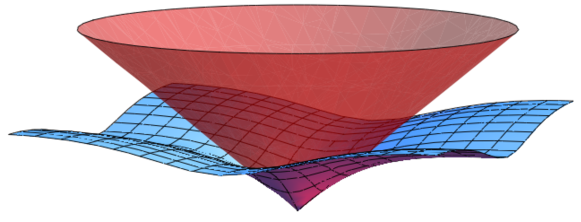
Figure 2: The energy surface of a massless, non-interacting Wilson fermion with $r=1$ as a function of momentum in the x and y directions, bounded by $-\pi<bp_{x,y}<\pi$, for $p_{z}=0$ is shown in blue. The continuum dispersion relation is shown as the red surface.

It is in the limit of small momentum, compared to the inverse lattice spacing, that the dispersion relations exhibit rotational invariance. While for the fundamental particles, the dispersion relations in eq. (16) and eq. (17) are valid, for composite particles, such as the proton or pion, the dispersion relations will be dynamically generated. In the present analysis we assume that the dispersion relations for all particles take the form of those in eq. (16) and eq. (17). It is also interesting to note that the polarizations of the massless vector fields are not exactly perpendicular to their direction of propagation for some directions of propagation with respect to the lattice axes, with longitudinal components present for non-zero lattice spacings.

Consider the process $p\rightarrow p+\gamma$, which is forbidden in the vacuum by energy-momentum conservation in special relativity when the speed of light of the proton and photon are equal, $c_{p}=c_{\gamma}$. Such a process can proceed in-medium when $v_{p}>c_{\gamma}$, corresponding to Cerenkov radiation. In the situation where the proton and photon have different MAV’s, the absence of this process in vacuum requires that $|c_{p}-c_{\gamma}|\raisebox{-3.01385pt}{$\stackrel{{\scriptstyle\textstyle<}}{{\sim}}$ }10^{-23}$ Coleman and Glashow (1997, 1999). In lattice simulations of the universe, this process could proceed in the vacuum if there are final state momenta which satisfy energy conservation for an initial state proton with energy $E_{i}$ moving in some direction with respect to the underlying cubic lattice. Numerically, we find that there are no final states that satisfy this condition, and therefore this process is forbidden for all proton momentum . In contrast, the process $\gamma\rightarrow e^{+}e^{-}$, which provides tight constraints on differences between MAV’s Coleman and Glashow (1999), can proceed for very high energy photons (those with energies comparable to the inverse lattice spacing) near the edges of the Brillouin zone. Further, very high energy $\pi^{0}$’s are stable against $\pi^{0}\rightarrow\gamma\gamma$, as is the related process $\gamma\rightarrow\pi^{0}\gamma$.

With the dispersion relation of special relativity, the structure of the cosmic ray spectrum is greatly impacted by the inelastic collisions of nucleons with the cosmic microwave background (CMB) Greisen (1966); Zatsepin and Kuzmin (1966). Processes such as $\gamma_{\rm CMB}+N\rightarrow\Delta$ give rise to the predicted GKZ-cut off scale Greisen (1966); Zatsepin and Kuzmin (1966) of $\sim 6\times 10^{20}~{}{\rm eV}$ in the spectrum of high energy cosmic rays. Recent experimental observations show a decline in the fluxes starting around this value Abraham et al. (2010); Sokolsky et al. (2010), indicating that the GKZ-cut off (or some other cut off mechanism) is present in the cosmic ray flux. For lattice spacings corresponding to an energy scale comparable to the GKZ cut off, the cosmic ray spectrum will exhibit significant deviations from isotropy, revealing the cubic structure of the lattice. However, for lattice spacings much smaller than the GKZ cut off scale, the GKZ mechanism cuts off the spectrum, effectively hiding the underlying lattice structure. When the lattice rest frame coincides with the CMB rest frame, head-on interactions between a high energy proton with momentum $|{\bf p}|$ and a photon of (very-low) energy $\omega$ can proceed through the $\Delta$ resonance when

$$\omega = {m_{\Delta}^{2}-m_{N}^{2}\over 4|{\bf p}|}\left[1+{\sqrt{\pi}b^{2}|{\bf p}|^{2}\over 9}\left(Y_{4}^{0}(\theta,\phi)\ +\ \sqrt{5\over 14}\left(Y_{4}^{+4}(\theta,\phi)\ +\ Y_{4}^{-4}(\theta,\phi)\right)\right)\right]$$ (18)

$$\ -\ {m_{\Delta}^{3}-m_{N}^{3}\over 4|{\bf p}|}br\ +\ ...\ \ \ ,$$

for $|{\bf p}|\ll 1/b$, where $\theta$ and $\phi$ are the polar and azimuthal angles of the particle momenta in the rest frame of the lattice, respectively. This represents a lower bound for the energy of photons participating in such a process with arbitrary collision angles.

The lattice spacing itself introduces a cut off to the cosmic ray spectrum. For both the fermions and the bosons, the cut off from the dispersion relation is $E^{\rm max}\sim 1/b$. Equating this to the GKZ cut off corresponds to a lattice spacing of $b\sim 10^{-12}~{}{\rm fm}$, or a mass scale of $b^{-1}\sim 10^{11}~{}{\rm GeV}$. Therefore, the lattice spacing used in the lattice simulation of the universe must be $b\raisebox{-3.01385pt}{$\stackrel{{\scriptstyle\textstyle<}}{{\sim}}$ }10^{-12}~{}{\rm fm}$ in order for the GZK cut off to be present or for the lattice spacing itself to provide the cut off in the cosmic ray spectrum. The most striking feature of the scenario in which the lattice provides the cut off to the cosmic ray spectrum is that the angular distribution of the highest energy components would exhibit cubic symmetry in the rest frame of the lattice, deviating significantly from isotropy. For smaller lattice spacings, the cubic distribution would be less significant, and the GKZ mechanism would increasingly dominate the high energy structure. It may be the case that more advanced simulations will be performed with non-cubic lattices. The results obtained for cubic lattices indicate that the symmetries of the non-cubic lattices should be imprinted, at some level, on the high energy cosmic ray spectrum.

V Conclusions

In this work, we have taken seriously the possibility that our universe is a numerical simulation. In particular, we have explored a number of observables that may reveal the underlying structure of a simulation performed with a rigid hyper-cubic space-time grid. This is motivated by the progress in performing lattice QCD calculations involving the fundamental fields and interactions of nature in femto-sized volumes of space-time, and by the simulation hypothesis of Bostrom Bostrom (2003). A number of elements required for a simulation of our universe directly from the fundamental laws of physics have not yet been established, and we have assumed that they will, in fact, be developed at some point in the future; two important elements being an algorithm for simulating chiral gauge theories, and quantum gravity. It is interesting to note that in the simulation scenario, the fundamental energy scale defined by the lattice spacing can be orders of magnitude smaller than the Planck scale, in which case the conflict between quantum mechanics and gravity should be absent.

The spectrum of the highest energy cosmic rays provides the most stringent constraint that we have found on the lattice spacing of a universe simulation, but precision measurements, particularly the muon $g-2$, are within a few orders of magnitude of being sensitive to the chiral symmetry breaking aspects of a simulation employing the unimproved Wilson lattice action. Given the ease with which current lattice QCD simulations incorporate improvement or employ discretizations that preserve chiral symmetry, it seems unlikely that any but the very earliest universe simulations would be unimproved with respect to the lattice spacing. Of course, improvement in this context masks much of our ability to probe the possibility that our universe is a simulation, and we have seen that, with the exception of the modifications to the dispersion relation and the associated maximum values of energy and momentum, even ${\cal O}(b^{2})$ operators in the Symanzik action easily avoid obvious experimental probes. Nevertheless, assuming that the universe is finite and therefore the resources of potential simulators are finite, then a volume containing a simulation will be finite and a lattice spacing must be non-zero, and therefore in principle there always remains the possibility for the simulated to discover the simulators.

Acknowledgments

We would like to thank Eric Adelberger, Blayne Heckel, David Kaplan, Kostas Orginos, Sanjay Reddy and Kenneth Roche for interesting discussions. We also thank William Detmold, Thomas Luu and Ann Nelson for comments on earlier versions of the manuscript. SRB was partially supported by the INT during the program INT-12-2b: Lattice QCD studies of excited resonances and multi-hadron systems, and by NSF continuing grant PHY1206498. In addition, SRB gratefully acknowledges the hospitality of HISKP and the support of the Mercator programme of the Deutsche Forschungsgemeinschaft. ZD and MJS were supported in part by the DOE grant DE-FG03-97ER4014.

References

- Bostrom (2003) N. Bostrom, Philosophical Quarterly, Vol 53, No 211, 243 (2003).
- Kronfeld (2012) A. S. Kronfeld, (2012), arXiv:1209.3468 [physics.hist-ph] .
- Fodor and Hoelbling (2012) Z. Fodor and C. Hoelbling, Rev.Mod.Phys., 84, 449 (2012), arXiv:1203.4789 [hep-lat] .
- Beane et al. (2012) S. R. Beane, E. Chang, S. D. Cohen, W. Detmold, H.-W. Lin, et al., (2012), arXiv:1206.5219 [hep-lat] .
- Yamazaki et al. (2012) T. Yamazaki, K.-i. Ishikawa, Y. Kuramashi, and A. Ukawa, (2012), arXiv:1207.4277 [hep-lat] .
- Aoki et al. (2012) S. Aoki et al. (HAL QCD Collaboration), (2012), arXiv:1206.5088 [hep-lat] .
- Lloyd (1999) S. Lloyd, Nature, 406, 1047 (1999), arXiv:quant-ph/9908043 [quant-ph] .
- Lloyd (2005) S. Lloyd, (2005), arXiv:quant-ph/0501135 [quant-ph] .
- Zuse (1969) K. Zuse, Rechnender Raum (Friedrich Vieweg and Sohn, Braunschweig, 1969).
- Fredkin (1990) E. Fredkin, Physica, D45, 254 (1990).
- Wolfram (2002) S. Wolfram, A New Kind of Science (Wolfram Media, 2002) p. 1197.
- ’t Hooft (2012) G. ’t Hooft, (2012), arXiv:1205.4107 [quant-ph] .
- Church (1936) J. Church, Am. J. Math, 58, 435 (1936).
- Turing (1936) A. Turing, Proc. Lond. Math Soc. Ser. 2, 442, 230 (1936).
- Deutsch (1985) D. Deutsch, Proc. of the Royal Society of London, A400, 97 (1985).
- Barrow (2008) J. Barrow, Living in a Simulated Universe, edited by B. Carr (Cambridge University Press, 2008) Chap. 27, Universe or Multiverse?, pp. 481–486.
- (17) MILC-Collaboration, http://physics.indiana.edu/sg/milc.html.
- Kogut and Susskind (1975) J. B. Kogut and L. Susskind, Phys.Rev., D11, 395 (1975).
- (19) SPECTRUM-Collaboration, http://usqcd.jlab.org/projects/AnisoGen/.
- Wilson (1974) K. G. Wilson, Phys.Rev., D10, 2445 (1974).
- Sheikholeslami and Wohlert (1985) B. Sheikholeslami and R. Wohlert, Nucl.Phys., B259, 572 (1985).
- Lin et al. (2009) H.-W. Lin et al. (Hadron Spectrum Collaboration), Phys.Rev., D79, 034502 (2009), arXiv:0810.3588 [hep-lat] .
- Vinge (1993) V. Vinge, Science and Engineering in the Era of Cyberspace, G. A. Landis, ed., NASA Publication CP-10129, Vision-21: Interdisciplinary, 115 (1993).
- Kurzweil (2006) R. Kurzweil, The Singularity Is Near: When Humans Transcend Biology (Penguin (Non-Classics), 2006) ISBN 0143037889.
- Coleman and Glashow (1999) S. R. Coleman and S. L. Glashow, Phys.Rev., D59, 116008 (1999), arXiv:hep-ph/9812418 [hep-ph] .
- Gagnon and Moore (2004) O. Gagnon and G. D. Moore, Phys.Rev., D70, 065002 (2004), arXiv:hep-ph/0404196 [hep-ph] .
- Collins et al. (2004) J. Collins, A. Perez, D. Sudarsky, L. Urrutia, and H. Vucetich, Phys.Rev.Lett., 93, 191301 (2004), arXiv:gr-qc/0403053 [gr-qc] .
- Kachru et al. (2003) S. Kachru, R. Kallosh, A. D. Linde, and S. P. Trivedi, Phys.Rev., D68, 046005 (2003), arXiv:hep-th/0301240 [hep-th] .
- Susskind (2003) L. Susskind, (2003), arXiv:hep-th/0302219 [hep-th] .
- Douglas (2003) M. R. Douglas, JHEP, 0305, 046 (2003), arXiv:hep-th/0303194 [hep-th] .
- Appelquist et al. (2012) T. Appelquist, R. C. Brower, M. I. Buchoff, M. Cheng, S. D. Cohen, et al., (2012), arXiv:1204.6000 [hep-ph] .
- Hsu and Zee (2006) S. Hsu and A. Zee, Mod.Phys.Lett., A21, 1495 (2006), arXiv:physics/0510102 [physics] .
- Symanzik (1983) K. Symanzik, Nucl.Phys., B226, 187 (1983a).
- Symanzik (1983) K. Symanzik, Nucl.Phys., B226, 205 (1983b).
- Aslanyan and Manohar (2012) G. Aslanyan and A. V. Manohar, JCAP, 1206, 003 (2012), arXiv:1104.0015 [astro-ph.CO] .
- Jizba et al. (2010) P. Jizba, H. Kleinert, and F. Scardigli, Phys.Rev., D81, 084030 (2010), arXiv:0912.2253 [hep-th] .
- Kaplan and Sun (2012) D. B. Kaplan and S. Sun, Phys.Rev.Lett., 108, 181807 (2012), arXiv:1112.0302 [hep-ph] .
- Lüscher and Weisz (1985) M. Lüscher and P. Weisz, Commun.Math.Phys., 97, 59 (1985).
- Mohr et al. (2012) P. J. Mohr, B. N. Taylor, and D. B. Newell, ArXiv e-prints (2012), arXiv:1203.5425 [physics.atom-ph] .
- Bouchendira et al. (2011) R. Bouchendira, P. Cladé, S. Guellati-Khélifa, F. Nez, and F. Biraben, Phys. Rev. Lett., 106, 080801 (2011).
- Colladay and Kostelecký (1997) D. Colladay and V. A. Kostelecký, Phys. Rev. D, 55, 6760 (1997).
- Myers and Pospelov (2003) R. C. Myers and M. Pospelov, Phys.Rev.Lett., 90, 211601 (2003), arXiv:hep-ph/0301124 [hep-ph] .
- Carroll et al. (1990) S. M. Carroll, G. B. Field, and R. Jackiw, Phys. Rev. D, 41, 1231 (1990).
- Laurent et al. (2011) P. Laurent, D. Gotz, P. Binetruy, S. Covino, and A. Fernandez-Soto, Phys.Rev., D83, 121301 (2011), arXiv:1106.1068 [astro-ph.HE] .
- Maccione et al. (2009) L. Maccione, A. M. Taylor, D. M. Mattingly, and S. Liberati, JCAP, 0904, 022 (2009), arXiv:0902.1756 [astro-ph.HE] .
- Motie and Xue (2012) I. Motie and S.-S. Xue, Int.J.Mod.Phys., A27, 1250104 (2012), arXiv:1206.0709 [hep-ph] .
- Xue (2011) S.-S. Xue, Phys.Lett., B706, 213 (2011), arXiv:1110.1317 [hep-ph] .
- Adam et al. (2011) T. Adam et al. (OPERA Collaboration), (2011), arXiv:1109.4897 [hep-ex] .
- Coleman and Glashow (1997) S. R. Coleman and S. L. Glashow, Phys.Lett., B405, 249 (1997), arXiv:hep-ph/9703240 [hep-ph] .
- Greisen (1966) K. Greisen, Phys.Rev.Lett., 16, 748 (1966).
- Zatsepin and Kuzmin (1966) G. Zatsepin and V. Kuzmin, JETP Lett., 4, 78 (1966).
- Abraham et al. (2010) J. Abraham et al. (Pierre Auger Collaboration), Phys.Lett., B685, 239 (2010), arXiv:1002.1975 [astro-ph.HE] .
- Sokolsky et al. (2010) P. Sokolsky et al. (HiRes Collaboration), PoS, ICHEP2010, 444 (2010), arXiv:1010.2690 [astro-ph.HE] .