Quantum polarization characterization and tomography

Abstract

We present a complete polarization characterization of any quantum state of two orthogonal polarization modes, and give a systematic measurement procedure to collect the necessary data. Full characterization requires measurements of the photon number in both modes and linear optics. In the situation where only the photon-number difference can be determined, a limited but useful characterization is obtained. The characteristic Stokes moment profiles are given for several common quantum states.

1 Introduction

Far from its source, any freely propagating electromagnetic field can be considered to a good approximation as a plane wave, with its electric field lying in a plane perpendicular to the direction of propagation. This simple observation is the root of the notion of polarization. At first glance, it may seem rather obvious how to translate such a concept into the realm of quantum optics. However, hurdles such as hidden polarization [1], the fact that the Poincaré sphere is too small to accommodate states with excitation larger than one photon [2], and the difficulties in defining polarization properties of two-photon entangled fields [3], to cite only a few examples, show that the classical theory, mainly based on first-order polarization moments, is insufficient for quantized fields.

Here, we outline a systematic method for polarization characterization of quantum fields. The method is based on a simple premise; namely, that if we can predict the $m$th-order moment of the Stokes operator in any direction on the Poincaré sphere, we know all there is to be known about the state polarization of this order [4], including any correlations between the Stokes operators. A tensor representation of the polarization information is based on such correlations. However, expressing the Stokes moments as functions of the measurement directions gives a more compact representation and provides a natural visualization. The Stokes profile representation also gives a relevant characterization for passive interferometry. Our analysis below makes use of both representations.

As a state’s polarization properties do not require the full density matrix to be determined, it allows polarization tomography to be more easily performed than full quantum tomography [5, 6, 7]. Considering polarization tomography with ideal detection, we show that the number of measurement directions can be made equal to the number of independent parameters.

The remaining material of the article is organized as follows. After recalling the fundamentals on the quantum description of polarization in section 2, we present our scheme for characterization of quantum polarization properties in section 3. In section 4, we consider how the necessary data can be obtained experimentally. We thus arrive at an efficient method, which is feasible for polarization tomography of few-photon states. In section 5, we apply our characterization to several classes of states. Finally, our conclusions are presented in section 6.

2 Setting the scene

In the following, we consider monochromatic plane waves. Such fields can be decomposed into two orthogonal transverse modes, such as the horizontally and vertically polarized modes. For highly focused beams or waves in a waveguide, the plane-wave description is often inadequate, as the field is not longer transverse. It is our belief that the concepts discussed in this paper can also be extended to such non-plane waves, and several proposals have already appeared in the literature [8, 9, 10]. However, we shall not discuss such generalizations here.

The classical theory for the polarization of plane waves was established by Stokes already more than 150 years ago [11]. We shall build on his theory as the basis of our treatment will be the Stokes operators, whose expectation values are the Stokes parameters [12]. Following the conventions used in the quantum theory of angular momentum [13] and in quantum optics [14, 15], we define the Stokes operators as

$$\begin{array}[]{ll}\hat{S}_{0}=\hat{a}_{H}^{\dagger}\hat{a}_{H}+\hat{a}_{V}^{\dagger}\hat{a}_{V}\,,&\hat{S}_{1}=\hat{a}_{H}\hat{a}_{V}^{\dagger}+\hat{a}_{H}^{\dagger}\hat{a}_{V}\,,\\ &\\ \hat{S}_{2}=i(\hat{a}_{H}\hat{a}_{V}^{\dagger}-\hat{a}_{H}^{\dagger}\hat{a}_{V})\,,&\hat{S}_{3}=\hat{a}_{H}^{\dagger}\hat{a}_{H}-\hat{a}_{V}^{\dagger}\hat{a}_{V}\,,\end{array}$$ (2.1)

where $\hat{a}_{H}$ and $\hat{a}_{V}$ are the annihilation operators of the modes associated with horizontally and vertically oscillating fields, respectively. With this choice, the usual ordering of the Stokes parameters $\mathcal{I}=\langle\hat{S}_{0}\rangle$, $\mathcal{Q}=\langle\hat{S}_{3}\rangle$, $\mathcal{U}=\langle\hat{S}_{1}\rangle$, and $\mathcal{V}=\langle\hat{S}_{2}\rangle$ differs from that of the indices of the operators. However, as far as the theory below is concerned, we could just as well have associated any other pair of orthogonal polarization modes to these operators. That would only influence the interpretation of the theory and not the theory itself.

As the annihilation and creation operators obey the bosonic commutation relations $[\hat{a}_{\alpha},\hat{a}_{\beta}^{\dagger}]=\delta_{\alpha\beta}$, for $\alpha,\beta\in\{H,V\}$, the Stokes operators satisfy the commutation relations of an su(2) algebra

$$[\hat{S}_{j},\hat{S}_{k}]=i2\,\varepsilon_{jk\ell}\hat{S}_{\ell}\,,$$ (2.2)

where the latin indices run from 1 to 3 and $\varepsilon_{jk\ell}$ is the fully antisymmetric Levi-Civita tensor. The noncommutability of these operators precludes the simultaneous exact measurement of the corresponding physical quantities. The variances $(\Delta S_{j})^{2}=\langle\hat{S}_{j}^{2}\rangle-\langle\hat{S}_{j}\rangle^{2}$ are found to obey the uncertainty relation

$$2\langle\hat{S}_{0}\rangle\leq(\Delta S_{1})^{2}+(\Delta S_{2})^{2}+(\Delta S_{3})^{2}\leq\langle\hat{S}_{0}(\hat{S}_{0}+2)\rangle\,.$$ (2.3)

Moreover, while the Stokes operators are all Hermitian, the noncommutability makes “mixed,” non-symmetric products (such as $\hat{S}_{1}\hat{S}_{2}$) non-Hermitian, also precluding their direct measurement.

The standard definition of the degree of polarization for a quantum state $\hat{\varrho}$ is

$$\mathbb{P}_{S}(\hat{\varrho})=\frac{|\langle\hat{\mathbf{S}}\rangle|}{\langle\hat{S}_{0}\rangle}=\frac{\sqrt{\langle\hat{S}_{1}\rangle^{2}+\langle\hat{S}_{2}\rangle^{2}+\langle\hat{S}_{3}\rangle^{2}}}{\langle\hat{S}_{0}\rangle}\,,$$ (2.4)

where $\hat{\mathbf{S}}=(\hat{S}_{1},\hat{S}_{2},\hat{S}_{3})$ and $\langle\hat{\mathbf{S}}\rangle$ is the Stokes vector. Note that only first-order moments of the Stokes operators are used in this definition. In a more elaborated characterization, the degree of polarization can be subdivided into excitation manifolds according to the total photon number $N$. This makes physical sense because since the corresponding observable $\hat{S}_{0}$ commutes with all the other Stokes operators

$$[\hat{S}_{0},\hat{S}_{j}]=0\,,$$ (2.5)

a complete set of simultaneous eigenstates of $\hat{S}_{0}$ and any of $\hat{S}_{1}$, $\hat{S}_{2}$, and $\hat{S}_{3}$ does exist. In fact, the statistics of the latter three operators is usually determined by a set of wave plates, a polarizing beam splitter, and two photodetectors, giving (in the ideal case) information not only about $\hat{S}_{1}$, $\hat{S}_{2}$, or $\hat{S}_{3}$, but simultaneously of $\hat{S}_{0}$.

Let us here take a quick look at excitation manifolds $N=1$ and $N=2$. One can readily convince oneself that any pure single-photon state $|\Psi_{1}\rangle$ satisfies $\mathbb{P}_{S}(|\Psi_{1}\rangle)=1$, i.e., any such state is fully polarized according to the definition (2.4). In fact, for an arbitrary single-photon state $\hat{\varrho}_{1}$, the degree of polarization is related to the purity $\Tr(\hat{\varrho}^{2})$ according to

$$\mathbb{P}_{S}(\hat{\varrho}_{1})=\sqrt{2\,\Tr(\hat{\varrho}_{1}^{2})-1}\,.$$ (2.6)

However, this relation does not hold for other excitation manifolds. For example, any pure state in excitation manifold $N=2$ of the form [16]

$$|\Psi(a,\theta)\rangle=ae^{-i\theta}|2,0\rangle+i\sqrt{1-2a^{2}}\,|1,1\rangle+ae^{i\theta}|0,2\rangle\,,$$ (2.7)

where $a$ and $\theta$ are real numbers and $0\leq a\leq 1/\sqrt{2}$, satisfies $\mathbb{P}_{S}(|\Psi(a,\theta)\rangle)=0$, which indicates that it is unpolarized. However, as we shall see below, these states have polarization structure (they are not isotropic in the polarization sense) and cannot be regarded as unpolarized.

3 Higher-order polarization properties

In order to characterize the polarization properties of a state, we shall employ measurements of higher-order moments of the Stokes operators. This is very close to the Glauber correlation functions in quantum coherence theory [17], and has common grounds with Klyshko generalized coherence matrices [1]. In a recent paper [4], we have used the central moments for higher-order polarization characterization. Whereas the central moments may be preferred by some readers, the raw moments used in the present work seem to allow for an easier and more systematic approach.

As we have already discussed, one can perform a measurement of the total photon number without disturbing the measurement of any other Stokes operator. In classical optics, this is tantamount to the fact that the state of polarization is independent of the intensity. This suggests that the polarization properties are given by $\hat{\mathbf{S}}$. However, an ideal measurement of polarization provides some information about the total energy and vice versa. For example, an even (odd) measured eigenvalue of any of the observables $\hat{S}_{1}$, $\hat{S}_{2}$, and $\hat{S}_{3}$ implies an even (odd) total number of photons. Also, determining the probability distribution for the total number of photons $p_{N}$ simultaneously sets bounds on the polarization properties in accordance with the inequalities (2.3).

Taking these observations into account, we distinguish polarization properties for different numbers of photons, and let full polarization characterization refer to complete knowledge of the expectation values of all possible combinations of the Stokes operators. The $r$th-order polarization information of a state $\hat{\varrho}$ is then given by $p_{N}$ and the expectation values of the form

$$T_{j_{1}j_{2}\ldots j_{r}}^{(r,N)}=\langle\hat{S}_{j_{1}}\hat{S}_{j_{2}}\ldots\hat{S}_{j_{r}}\rangle_{N}=\Tr(\hat{\varrho}_{N}\hat{S}_{j_{1}}\hat{S}_{j_{2}}\ldots\hat{S}_{j_{r}})\,,$$ (3.1)

where $j_{k}\in\{1,2,3\}$ and $\hat{\varrho}_{N}$ denotes the normalized two-mode, $N$-photon state obtained by projecting $\hat{\varrho}$ onto the $N$th excitation manifold

$$\hat{\varrho}_{N}=\frac{\hat{\leavevmode\hbox{\small 1\normalsize\kern-3.30002pt1}}_{N}\hat{\varrho}\hat{\leavevmode\hbox{\small 1\normalsize\kern-3.30002pt1}}_{N}}{p_{N}}\,.$$ (3.2)

Using the Fock basis, the projector can thus be expressed as $\hat{\leavevmode\hbox{\small 1\normalsize\kern-3.30002pt1}}_{N}=\sum_{n=0}^{N}|n,N-n\rangle\langle n,N-n|$ and $p_{N}=\Tr(\hat{\leavevmode\hbox{\small 1\normalsize\kern-3.30002pt1}}_{N}\hat{\varrho})$. For any given order $r$ and excitation manifold $N$, the elements (3.1) form a Cartesian tensor $\mathbf{T}^{(r,N)}(\hat{\varrho})$ of rank $r$. Due to the Hermiticity of the Stokes operators, theses tensors satisfy

$$T_{j_{1}\ldots j_{r}}^{(r,N)}=[T_{j_{r}\ldots j_{1}}^{(r,N)}]^{\ast}\,.$$ (3.3)

We leave $\hat{\varrho}_{N}$ and $\mathbf{T}^{(r,N)}$ undefined for any $N$ such that $p_{N}=0$, and employ the convention that they then do not contribute to sums.

When $(\mu,\nu,j_{k})$ is a cyclic permutation of $(1,2,3)$, the commutation relation (2.2) implies that polarization tensor elements of neighboring ranks are related according to

$$T_{j_{1}\ldots\mu\nu\ldots j_{r-1}}^{(r,N)}-T_{j_{1}\ldots\nu\mu\ldots j_{r-1}}^{(r,N)}=i2\,T_{j_{1}\ldots j_{k}\ldots j_{r-1}}^{(r-1,N)}\,.$$ (3.4)

Hence, $\mathbf{T}^{(r-1,N)}$ can be determined from $\mathbf{T}^{(r,N)}$ and, consequently, $\mathbf{T}^{(R,N)}$ determines all $\mathbf{T}^{(r,N)}$ such that $r<R$. Complete polarization information of order $R$ is thus equivalent to complete polarization information of all orders $r\leq R$.

Using the relations (2.1) and (2.2), it is also straightforward to show that the polarization information carried by $\mathbf{T}^{(R,N)}$ is equivalent to that contained in the set of generalized coherence matrices of orders $2r$ ($r\leq R$), whose elements are of the form [1] $\langle(\hat{a}_{H}^{\dagger})^{j}(\hat{a}_{V}^{\dagger})^{r-j}\hat{a}_{H}^{k}\hat{a}_{V}^{r-k}\rangle_{N}$. Having complete polarization information of all orders about a state $\hat{\varrho}$ is therefore equivalent to knowing its block-diagonal projection [16, 5, 7, 18]

$$\hat{\varrho}_{\mathrm{pol}}=\sum_{N=0}^{\infty}p_{N}\hat{\varrho}_{N}\,,\\$$ (3.5)

where $\hat{\varrho}_{N}$ is given by (3.2). This is the so called the polarization sector (or polarization density matrix). The number of parameters characterizing a block-diagonal state limited to the excitation manifolds $N_{1},N_{2},\ldots,N_{\nu}$ is

$$-1+\sum_{k=1}^{\nu}(N_{k}+1)^{2}.$$ (3.6)

In particular, when a state is limited to the manifolds $0,1,\ldots,\widetilde{N}$, the number of parameters simplifies to

$$-1+\sum_{N=0}^{\widetilde{N}}(N+1)^{2}=\frac{\widetilde{N}(2\widetilde{N}^{2}+9\widetilde{N}+13)}{6}.$$ (3.7)

For such a state, complete polarization information of order $\widetilde{N}$ is sufficient to determine its block-diagonal projection (3.5). The general density matrix for a state with no more than $\widetilde{N}$ photons is determined by $\widetilde{N}(\widetilde{N}+3)(\widetilde{N}^{2}+3\widetilde{N}+4)/4$ independent real numbers. Hence, the polarization share of this information quickly decreases with $\widetilde{N}$.

4 Polarization tomography

We now turn to the question of how to characterize polarization properties experimentally. Since our interest is limited to the information contained in the block-diagonal projection (3.5), it is clear that we are not required to do full quantum state tomography [5, 7, 6]. As complete polarization information corresponds to doing quantum tomography of all $N$-photon Hilbert spaces excited by the considered state, one can make use of the methods developed for finite-dimensional systems [19, 20, 21]. However, some recently proposed higher-order intensity measurements [22] seem to be closest related to the ones we present below.

We will assume ideal measurements and that the total photon number and its probability distribution $p_{N}$ can be determined. This is obviously a severe restriction apart from the lowest excitation manifolds. However, the situation where no information about the total photon number can be obtained is described by simply summing over the different manifolds as discussed in section 4.4.

Below, we also treat the experimental determination of different moments of an observable as different measurements. In principle, each moment requires an infinite number of measurement runs in order to be determined exactly. This would also give us the full probability distribution of the eigenvalues and thus all the moments. However, for the vast majority of realistic probability distributions, a lower moment requires fewer runs to be accurately determined.

4.1 Moment measurements

The fact that the classical Stokes parameters are easily determined experimentally makes them highly practical. Also in quantum optics, the measurement setups corresponding to the fundamental Stokes operators are simple. These setups are composed only by phase shifters, beam splitters and photon-number measurements. The effects of linear optical devices are described by SU(2) transformations [14], which can be expressed as

$$\hat{U}(\Phi,\Theta,\Xi)=e^{-i\Phi\hat{S}_{3}/2}e^{-i\Theta\hat{S}_{2}/2}e^{-i\Xi\hat{S}_{3}/2},$$ (4.1)

where $\Phi$, $\Theta$, and $\Xi$ are the Euler angles. Any such transformation can be easily realized using linear optics [23] and they are lossless, so they leave $\hat{S}_{0}$ unaffected.

Let us now introduce the Stokes operator in an arbitrary direction characterized by the unit vector $\mathbf{n}\in\mathbb{R}^{3}$ as

$$\hat{S}_{\mathbf{n}}\equiv\mathbf{n}\cdot\hat{\mathbf{S}}=\sum_{k=1}^{3}n_{k}\hat{S}_{k}.$$ (4.2)

The effect of an arbitrary SU(2) transformation on $\hat{S}_{\mathbf{n}}$, can then be expressed as

$$\hat{U}(\Phi,\Theta,\Xi)\,\hat{S}_{\mathbf{n}}\,\hat{U}^{\dagger}(\Phi,\Theta,\Xi)=\hat{S}_{\mathbf{R}_{3}(\Phi)\cdot\mathbf{R}_{2}(\Theta)\cdot\mathbf{R}_{3}(\Xi)\cdot\mathbf{n}},\qquad$$ (4.3)

where $\mathbf{R}_{k}(\phi)$ denotes the matrix describing a rotation of $\phi$ around the $\mathbf{e}_{k}$-axis, e.g.

$$\mathbf{R}_{1}(\phi)=\left[\begin{array}[]{ccc}1&0&0\cr 0&\cos\phi&-\sin\phi\cr 0&\sin\phi&\cos\phi\end{array}\right].$$ (4.4)

Hence, any SU(2) transformation corresponds to a proper rotation in $\mathbb{R}^{3}$ [14]. We note that $\hat{S}_{3}$, which gives the photon-number difference, is transformed according to

$$\hat{U}(\Phi,\Theta,\Xi)\,\hat{S}_{3}\,\hat{U}^{\dagger}(\Phi,\Theta,\Xi)=\hat{S}_{\mathbf{n}},\quad\quad\quad\mathbf{n}=(\sin\Theta\cos\Phi,\sin\Theta\sin\Phi,\cos\Theta).$$ (4.5)

That is, $\hat{U}(\Phi,\Theta,0)$ is the standard displacement on the sphere and the transformation parameters $\Theta$ and $\Phi$ equal the spherical coordinates of the vector $\mathbf{n}$ characterizing the transformed Stokes operator. We see that any $\hat{S}_{\mathbf{n}}$ is related to $\hat{S}_{3}$ by an SU(2) transformation corresponding to a polarization rotation of $\Theta/2$ followed by a differential phase shift of $\Phi/2$. Expectation values of the form $\langle\hat{S}_{\mathbf{n}}^{r}\rangle$ can thus be straightforwardly determined experimentally. Ideally, we can simultaneously measure the total photon number $N$, so that also expectation values of the form $\langle\hat{S}_{\mathbf{n}}^{r}\rangle_{N}$ can be determined.

The tensor $\mathbf{T}^{(r,N)}$ gives any expectation value of the form

$$\langle\hat{S}_{\mathbf{n}_{1}}\hat{S}_{\mathbf{n}_{2}}\ldots\hat{S}_{\mathbf{n}_{r}}\rangle_{N}=\sum_{j_{1}=1}^{3}\ldots\sum_{j_{r}=1}^{3}n_{j_{1}}^{(1)}\ldots n_{j_{r}}^{(r)}T_{j_{1}\ldots j_{r}}^{(r,N)}\,.$$ (4.6)

When all vectors are the same, (4.6) simplifies considerably. For a given state, the relation between $\langle\hat{S}_{\mathbf{n}}^{r}\rangle_{N}$ and the direction $\mathbf{n}$ will be referred to as the $N$-photon Stokes moment profile of order $r$. These profiles can be expressed as

$$\langle\hat{S}_{\mathbf{n}}^{r}\rangle_{N}=\sum_{k=0}^{r}\sum_{\ell=0}^{r-k}n_{1}^{k}n_{2}^{\ell}n_{3}^{r-k-\ell}M_{k,\ell}^{(r,N)}\ ,$$ (4.7)

where the moment component $M_{k,\ell}^{(r,N)}$ is the sum of all tensor elements of the form $T_{j_{1}\ldots j_{r}}^{(r,N)}$ that have $k$ ones and $\ell$ twos as subscripts. Due to (3.1), every moment component is thus the expectation value of the Hermitian operator formed by the sum of the Stokes-operator products corresponding to its tensor elements. The number of such elements is given by the trinomial coefficient

$$(k,\ell,r-k-\ell)!=\frac{r!}{k!\ell!(r-k-\ell)!}.$$ (4.8)

For example, we have $M_{1,1}^{(3,N)}=T_{123}^{(3,N)}+T_{132}^{(3,N)}+T_{213}^{(3,N)}+T_{231}^{(3,N)}+T_{312}^{(3,N)}+T_{321}^{(3,N)}$. We note that the sum of all tensor elements of order $r$ in excitation manifold $N$ can be written as

$$\sum_{j_{1}=1}^{3}\ldots\sum_{j_{r}=1}^{3}T_{j_{1}\ldots j_{r}}^{(r,N)}=\sum_{k=0}^{r}\sum_{\ell=0}^{r-k}M_{k,\ell}^{(r,N)}=3^{r/2}\langle\hat{S}_{\mathbf{n}_{\mathrm{diag}}}^{r}\rangle_{N}\,,$$ (4.9)

where $\mathbf{n}_{\mathrm{diag}}=(1,1,1)/\sqrt{3}$.

Since the polarization tensor satisfies the Hermiticity condition (3.3), the moment components are real, and consequently the real part of $\mathbf{T}^{(r,N)}$ is sufficient to determine $\langle\hat{S}_{\mathbf{n}}^{r}\rangle_{N}$ in any direction $\mathbf{n}$. Naturally, knowing the Stokes moment profile (4.7) is equivalent to knowing the

$$m_{r}=\frac{(r+1)(r+2)}{2}$$ (4.10)

moment components $M_{k,\ell}^{(r,N)}$.

Moreover, using the commutation relation (2.2), it is possible to determine the differences between the tensor elements belonging to the same moment component $M_{k,\ell}^{(r,N)}$ from $\mathbf{T}^{(r-1,N)}$. Since every element of $\mathbf{T}^{(r,N)}$ belongs to such a moment component, it thus follows that $\mathbf{T}^{(r-1,N)}$ together with all $M_{k,\ell}^{(r,N)}$ determine $\mathbf{T}^{(r,N)}$.

Let us now introduce a standard ordering of the Stokes operators according to

$$\hat{\mathcal{O}}_{k,\ell}^{(r)}=\hat{S}_{1}^{k}\hat{S}_{2}^{\ell}\hat{S}_{3}^{r-k-\ell}.$$ (4.11)

Making repeated use of the commutation relation (2.2), the moment components can then be expressed as

$$M_{k,\ell}^{(r,N)}=(k,\ell,r-k-\ell)!\,\langle\hat{\mathcal{O}}_{k,\ell}^{(r)}\rangle_{N}+\langle\hat{\mathcal{C}}_{k,\ell}^{(r)}\rangle_{N}\,,$$ (4.12)

where $\hat{\mathcal{C}}_{k,\ell}^{(r)}$ is a sum over Stokes-operator products of orders smaller than $r$. The Casimir operator

$$\hat{\mathbf{S}}^{2}=\sum_{k=1}^{3}\hat{S}_{k}^{2}=\hat{S}_{0}(\hat{S}_{0}+2)$$ (4.13)

implies that, for $r\geq 2$, we have

$$\langle\hat{\mathcal{O}}_{k+2,\ell}^{(r)}\rangle_{N}+\langle\hat{\mathcal{O}}_{k,\ell+2}^{(r)}\rangle_{N}+\langle\hat{\mathcal{O}}_{k,\ell}^{(r)}\rangle_{N}=N(N+2)\langle\hat{\mathcal{O}}_{k,\ell}^{(r-2)}\rangle_{N}+\langle\hat{S}_{1}^{k}[\hat{S}_{1}^{2},\hat{S}_{2}^{\ell}]\hat{S}_{3}^{r-k-\ell-2}\rangle_{N}\,,$$ (4.14)

where the last term can again be written as a sum over Stokes-operator products of orders smaller than $r$. Equations (4.12) and (4.14) show that there is a relation between moment components of orders $r$ and $r-2$, and that the number of independent moment components of order $r$ is $m_{r}-m_{r-2}=2r+1$. For a general $N$-photon state, the number of independent moment components to determine is thus $\sum_{r=1}^{N}(2r+1)=N(N+2)$. For a general block-diagonal state, we also have to determine the probability distribution for the total number of photons. Assuming that the excited manifolds are known to be limited to $N_{1},N_{2},\ldots,N_{\nu}$, we find the number of independent parameters to be $\nu-1+\sum_{k=1}^{\nu}N_{k}(N_{k}+2)$, which is in agreement with (3.6).

4.1.1 General single-photon state

In the basis $(|1,0\rangle,|0,1\rangle)$, the density matrix of a general single-photon state can be written as

$$\hat{\varrho}_{1}=\left(\begin{array}[]{cc}\pi_{0}&R+iI\cr R-iI&1-\pi_{0}\end{array}\right),$$ (4.15)

where $R^{2}+I^{2}\leq\pi_{0}(1-\pi_{0})$. Using a superscript to identify state-specific average values, the first-order Stokes moment profile is given by

$$\langle\hat{S}_{\mathbf{n}}\rangle_{1}^{\hat{\varrho}_{1}}=2Rn_{1}-2In_{2}+(2\pi_{0}-1)n_{3}.$$ (4.16)

Hence, the three moment components are seen to be independent.

4.1.2 General two-photon state

Using the basis $(|2,0\rangle,|1,1\rangle,|0,2\rangle)$, the density matrix of a general two-photon state can be written as

$$\hat{\varrho}_{2}=\left(\begin{array}[]{ccc}\pi_{1}&R_{1}+iI_{1}&R_{2}+iI_{2}\cr R_{1}-iI_{1}&\pi_{2}&R_{3}+iI_{3}\\ R_{2}-iI_{2}&R_{3}-iI_{3}&1-\pi_{1}-\pi_{2}\end{array}\right)\,.$$ (4.17)

The first- and second-order Stokes moment profiles can then be expressed as

$$\langle\hat{S}_{\mathbf{n}}\rangle_{2}^{\hat{\varrho}_{2}} = 2\sqrt{2}\,[(R_{1}+R_{3})n_{1}-(I_{1}+I_{3})n_{2}]+2\,(2\pi_{1}+\pi_{2}-1)n_{3},$$ (4.18)

$$\langle\hat{S}_{\mathbf{n}}^{2}\rangle_{2}^{\hat{\varrho}_{2}} = 2\,(1+\pi_{2}+2R_{2})n_{1}^{2}+2\,(1+\pi_{2}-2R_{2})n_{2}^{2}+4\,(1-\pi_{2})n_{3}^{2}-8I_{2}n_{1}n_{2}$$ (4.19)

$$+ 4\sqrt{2}\,n_{3}[(R_{1}-R_{3})n_{1}-(I_{1}-I_{3})n_{2}],$$

which makes it easy to identify the moment components. As implied by (4.13), the moment components of the three first terms of (4.19) are determined by two parameters. Hence, there are only five independent second-order moment components.

4.2 Choosing measurement directions

We have seen that the information content of the moment components allows us to do polarization tomography by only measuring moments. Performing the moment measurements in increasing order, the $2r+1$ independent moment components for each order $r$ and manifold $N$ can be determined by choosing equally many directions $\mathbf{n}$ such that (4.7) gives linearly independent equations for the unknown moment components.

4.2.1 First order

Quite naturally, both the first-order moment components and the first-order polarization tensors are given by the manifold-specific Stokes parameters

$$M_{\delta_{1j},\delta_{2j}}^{(1,N)}=T_{j}^{(1,N)}=\langle\hat{S}_{j}\rangle_{N}\,.$$ (4.20)

The three sets of information are hence identical and are obtained by determining the expectation value $\langle\hat{S}_{\mathbf{n}}\rangle_{N}$ for the directions $\mathbf{n}=(1,0,0)$, $(0,1,0)$, and $(0,0,1)$. As the operators $\hat{S}_{\mathbf{n}}$ and $\hat{S}_{-\mathbf{n}}$ only differ by the signs of their eigenvalues, the corresponding measurements will give the same information. Hence, equivalent measurements correspond to a line through the origin. Choosing three orthogonal directions as above thus results in a uniform distribution of the measurements on the Poincaré sphere.

4.2.2 Second order

We have seen that there are five independent moment components of second order. Thinking of the measurements as lines, we choose the directions as

$$\mathbf{n}_{1,2}=\frac{(0,\pm 2,1+\sqrt{5})}{\sqrt{10+2\sqrt{5}}},\qquad\mathbf{n}_{3,4}=\frac{(\pm 2,1+\sqrt{5},0)}{\sqrt{10+2\sqrt{5}}},\qquad\mathbf{n}_{5}=\frac{(1+\sqrt{5},0,2)}{\sqrt{10+2\sqrt{5}}}\,,$$ (4.21)

which maximizes the minimum angle between the lines [24, 25] and thus in some sense spreads out the measurements over the Poincaré sphere as much as possible. The six second-order moment components are then given by

$$M_{0,1}^{(2,N)}=\frac{\sqrt{5}}{2}\langle\hat{S}_{\mathbf{n}_{1}}^{2}-\hat{S}_{\mathbf{n}_{2}}^{2}\rangle_{N},$$ (4.22)

$$M_{1,1}^{(2,N)}=\frac{\sqrt{5}}{2}\langle\hat{S}_{\mathbf{n}_{3}}^{2}-\hat{S}_{\mathbf{n}_{4}}^{2}\rangle_{N},$$ (4.23)

$$M_{1,0}^{(2,N)}=\frac{\sqrt{5}}{2}\langle\hat{S}_{\mathbf{n}_{1}}^{2}+\hat{S}_{\mathbf{n}_{2}}^{2}+\hat{S}_{\mathbf{n}_{3}}^{2}+\hat{S}_{\mathbf{n}_{4}}^{2}+2\hat{S}_{\mathbf{n}_{5}}^{2}\rangle_{N}-\sqrt{5}N(N+2),$$ (4.24)

$$M_{0,0}^{(2,N)}=\frac{(15+7\sqrt{5})\langle\hat{S}_{\mathbf{n}_{1}}^{2}+\hat{S}_{\mathbf{n}_{2}}^{2}\rangle_{N}-(10+4\sqrt{5})\langle\hat{S}_{\mathbf{n}_{3}}^{2}+\hat{S}_{\mathbf{n}_{4}}^{2}\rangle_{N}+(6+2\sqrt{5})N(N+2)}{4(7+3\sqrt{5})},$$ (4.25)

$$M_{0,2}^{(2,N)}=\frac{(10+4\sqrt{5})\langle\hat{S}_{\mathbf{n}_{1}}^{2}+\hat{S}_{\mathbf{n}_{2}}^{2}\rangle_{N}+(25+11\sqrt{5})\langle\hat{S}_{\mathbf{n}_{3}}^{2}+\hat{S}_{\mathbf{n}_{4}}^{2}\rangle_{N}-(14+6\sqrt{5})N(N+2)}{4(7+3\sqrt{5})},$$ (4.26)

$$M_{2,0}^{(2,N)}=\frac{(36+16\sqrt{5})N(N+2)-(25+11\sqrt{5})\langle\hat{S}_{\mathbf{n}_{1}}^{2}+\hat{S}_{\mathbf{n}_{2}}^{2}\rangle_{N}-(15+7\sqrt{5})\langle\hat{S}_{\mathbf{n}_{3}}^{2}+\hat{S}_{\mathbf{n}_{4}}^{2}\rangle_{N}}{4(7+3\sqrt{5})}.$$ (4.27)

Note that their determination does not require any first-order measurement. The second-order polarization tensors can be expressed in the first- and second-order moment components as

$$\mathbf{T}^{(2,N)}=\left(\begin{array}[]{ccc}M_{2,0}^{(2,N)}&\frac{M_{1,1}^{(2,N)}}{2}+i\langle\hat{S}_{3}\rangle_{N}&\frac{M_{1,0}^{(2,N)}}{2}-i\langle\hat{S}_{2}\rangle_{N}\\ \frac{M_{1,1}^{(2,N)}}{2}-i\langle\hat{S}_{3}\rangle_{N}&M_{0,2}^{(2,N)}&\frac{M_{0,1}^{(2,N)}}{2}+i\langle\hat{S}_{1}\rangle_{N}\\ \frac{M_{1,0}^{(2,N)}}{2}+i\langle\hat{S}_{2}\rangle_{N}&\frac{M_{0,1}^{(2,N)}}{2}+i\langle\hat{S}_{1}\rangle_{N}&M_{0,0}^{(2,N)}\end{array}\right).$$ (4.31)

When writing tensors, we let larger entities and rows correspond to tensor indices placed to the left of those corresponding to smaller entities and columns.

As an aside, we decompose the Stokes-operator covariance matrix into different excitation manifolds $\bm{\Gamma}=\sum_{N=0}^{\infty}p_{N}\bm{\Gamma}_{N}$ and note that the matrix elements are given by

$$\Gamma_{jk,N}\equiv\frac{\langle\hat{S}_{j}\hat{S}_{k}\rangle_{N}+\langle\hat{S}_{k}\hat{S}_{j}\rangle_{N}}{2}-\langle\hat{S}_{j}\rangle_{N}\langle\hat{S}_{k}\rangle_{N}=\mathrm{Re}(T_{jk}^{(2,N)})-T_{j}^{(1,N)}T_{k}^{(1,N)}.$$ (4.32)

For any state that satisfies $\mathbb{P}_{S}=0$, we thus have $\bm{\Gamma}_{N}=\mathrm{Re}(\mathbf{T}^{(2,N)})$.

4.2.3 Third order

We know that there are seven independent third-order moment components. Maximizing the minimum angle between seven lines [25], we find that the measurements should correspond to $\hat{S}_{1}$, $\hat{S}_{2}$, $\hat{S}_{3}$, and the directions

$$\mathbf{n}_{4,5}=\frac{(\pm 1,1,1)}{\sqrt{3}},\quad\quad\quad\mathbf{n}_{6,7}=\frac{(\pm 1,-1,1)}{\sqrt{3}}.$$ (4.33)

However, this choice gives only four independent measurements, since we have

$$\hat{S}_{1}^{3}=\frac{3\sqrt{3}}{8}\,(-\hat{S}_{\mathbf{n}_{4}}^{3}+\hat{S}_{\mathbf{n}_{5}}^{3}-\hat{S}_{\mathbf{n}_{6}}^{3}+\hat{S}_{\mathbf{n}_{7}}^{3})+\frac{3N(N+2)-4}{2}\,\hat{S}_{1}$$ (4.34)

and similar relations for $\hat{S}_{2}^{3}$ and $\hat{S}_{3}^{3}$. By choosing directions close to $\hat{S}_{1}$, $\hat{S}_{2}$, and $\hat{S}_{3}$, it is possible to determine all third-order moment components. However, this choice would make it hard to obtain the necessary data, since the corresponding expectation values differ only slightly from the known $\langle\hat{S}_{1}^{3}\rangle_{N}$, $\langle\hat{S}_{2}^{3}\rangle_{N}$, and $\langle\hat{S}_{3}^{3}\rangle_{N}$. Consequently, although highly symmetric polyhedrons have been successfully applied in protocols for tomography of multi-qubit states [26], the related method considered here fails. How to optimally choose the measurement directions for higher-order polarization tomography thus appears to be a complicated problem. This notwithstanding, the third-order polarization tensors can be expressed as

$$\mathbf{T}^{(3,N)}=\left(\begin{array}[]{ccc}M_{3,0}^{(3,N)}&\frac{M_{2,1}^{(3,N)}+i4T_{1,3}^{(2,N)}+i2T_{3,1}^{(2,N)}}{3}&\frac{M_{2,0}^{(3,N)}-i4T_{1,2}^{(2,N)}-i2T_{2,1}^{(2,N)}}{3}\cr\frac{M_{2,1}^{(3,N)}-i2T_{1,3}^{(2,N)}+i2T_{3,1}^{(2,N)}}{3}&\frac{M_{1,2}^{(3,N)}+i2T_{2,3}^{(2,N)}+i4T_{3,2}^{(2,N)}}{3}&\frac{M_{1,1}^{(3,N)}}{6}+iT_{1,1}^{(2,N)}-iT_{2,2}^{(2,N)}+iT_{3,3}^{(2,N)}\cr\frac{M_{2,0}^{(3,N)}+i2T_{1,2}^{(2,N)}-i2T_{2,1}^{(2,N)}}{3}&\frac{M_{1,1}^{(3,N)}}{6}-iT_{1,1}^{(2,N)}-iT_{2,2}^{(2,N)}+iT_{3,3}^{(2,N)}&\frac{M_{1,0}^{(3,N)}-i2T_{3,2}^{(2,N)}-i4T_{2,3}^{(2,N)}}{3}\cr\hline\cr\frac{M_{2,1}^{(3,N)}-i2T_{1,3}^{(2,N)}-i4T_{3,1}^{(2,N)}}{3}&\frac{M_{1,2}^{(3,N)}+i2T_{2,3}^{(2,N)}-i2T_{3,2}^{(2,N)}}{3}&\frac{M_{1,1}^{(3,N)}}{6}+iT_{1,1}^{(2,N)}-iT_{2,2}^{(2,N)}-iT_{3,3}^{(2,N)}\cr\frac{M_{1,2}^{(3,N)}-i4T_{2,3}^{(2,N)}-i2T_{3,2}^{(2,N)}}{3}&M_{0,3}^{(3,N)}&\frac{M_{0,2}^{(3,N)}+i4T_{2,1}^{(2,N)}+i2T_{1,2}^{(2,N)}}{3}\cr\frac{M_{1,1}^{(3,N)}}{6}+iT_{1,1}^{(2,N)}+iT_{2,2}^{(2,N)}-iT_{3,3}^{(2,N)}&\frac{M_{0,2}^{(3,N)}-i2T_{2,1}^{(2,N)}+i2T_{1,2}^{(2,N)}}{3}&\frac{M_{0,1}^{(3,N)}+i2T_{3,1}^{(2,N)}+i4T_{1,3}^{(2,N)}}{3}\cr\hline\cr\frac{M_{2,0}^{(3,N)}+i2T_{1,2}^{(2,N)}+i4T_{2,1}^{(2,N)}}{3}&\frac{M_{1,1}^{(3,N)}}{6}-iT_{1,1}^{(2,N)}+iT_{2,2}^{(2,N)}+iT_{3,3}^{(2,N)}&\frac{M_{1,0}^{(3,N)}-i2T_{3,2}^{(2,N)}+i2T_{2,3}^{(2,N)}}{3}\cr\frac{M_{1,1}^{(3,N)}}{6}-iT_{1,1}^{(2,N)}+iT_{2,2}^{(2,N)}-iT_{3,3}^{(2,N)}&\frac{M_{0,2}^{(3,N)}-i2T_{2,1}^{(2,N)}-i4T_{1,2}^{(2,N)}}{3}&\frac{M_{0,1}^{(3,N)}+i2T_{3,1}^{(2,N)}-i2T_{1,3}^{(2,N)}}{3}\cr\frac{M_{1,0}^{(3,N)}+i4T_{3,2}^{(2,N)}+i2T_{2,3}^{(2,N)}}{3}&\frac{M_{0,1}^{(3,N)}-i4T_{3,1}^{(2,N)}-i2T_{1,3}^{(2,N)}}{3}&M_{0,0}^{(3,N)}\end{array}\right).$$ (4.35)

4.3 Recurrence relation for Stokes moment profiles

Above, we have seen that the $N$ lowest-order Stokes moment profiles $\{\langle\hat{S}_{\mathbf{n}}^{r}\rangle_{N}\}_{r=1}^{N}$ contain all polarization information of an $N$-photon state. In particular, we show in the appendix that the higher-order profiles are determined by the recurrence relation

$$\langle\hat{S}_{\mathbf{n}}^{N+1+\mu}\rangle_{N}=\left\{\begin{array}[]{ll}\displaystyle-\sum_{j=1}^{N/2}4^{N/2+1-j}f(N+2,2j)\,\langle\hat{S}_{\mathbf{n}}^{2j-1+\mu}\rangle_{N},&N\ \mathrm{even,}\\ \displaystyle-\sum_{j=0}^{\frac{N-1}{2}}4^{\frac{N+1}{2}-j}f(N+2,2j+1)\,\langle\hat{S}_{\mathbf{n}}^{2j+\mu}\rangle_{N},&N\ \mathrm{odd,}\end{array}\right.$$ (4.36)

where $\mu$ is a non-negative integer and $f(n,k)$ are the central factorial numbers of the first kind given by [27]

$$f(n,k)=\left\{\begin{array}[]{ll}0,&n<k,\\ \delta_{n,0},&k=0,\\ \displaystyle{2n-k\choose k}k\sum_{j=0}^{n-k}\frac{(-1)^{j}}{j!(n+j)}{2n-2k\choose n-k-j}\sum_{m=0}^{j}(-1)^{m}{j\choose m}\left(\frac{j}{2}-m\right)^{n-k+j},&1\leq k\leq n.\end{array}\right.$$ (4.37)

For the lowest excitation manifolds, we thus get

$$\begin{array}[]{ll}\langle\hat{S}_{\mathbf{n}}^{r}\rangle_{0}=0,&\langle\hat{S}_{\mathbf{n}}^{r}\rangle_{1}=\left\{\begin{array}[]{ll}1,&r\ \mathrm{even,}\\ \langle\hat{S}_{\mathbf{n}}\rangle_{1},&r\ \mathrm{odd,}\end{array}\right.\\[17.07182pt] \langle\hat{S}_{\mathbf{n}}^{r}\rangle_{2}=\left\{\begin{array}[]{ll}2^{r-2}\langle\hat{S}_{\mathbf{n}}^{2}\rangle_{2},&r\ \mathrm{even,}\\ 2^{r-1}\langle\hat{S}_{\mathbf{n}}\rangle_{2},&r\ \mathrm{odd,}\end{array}\right.&\langle\hat{S}_{\mathbf{n}}^{r}\rangle_{3}=\left\{\begin{array}[]{ll}\frac{9-3^{r}+(3^{r}-1)\langle\hat{S}_{\mathbf{n}}^{2}\rangle_{3}}{8},&r\ \mathrm{even,}\\ \frac{(9-3^{r-1})\langle\hat{S}_{\mathbf{n}}\rangle_{3}+(3^{r-1}-1)\langle\hat{S}_{\mathbf{n}}^{3}\rangle_{3}}{8},&r\ \mathrm{odd.}\end{array}\right.\end{array}$$ (4.46)

The above relations for $N=1$ and $N=2$ can also be established from the general property

$$\hat{S}_{-\mathbf{n}}^{r}=\left\{\begin{array}[]{rl}\hat{S}_{\mathbf{n}}^{r},&r\ \mathrm{even,}\\ -\hat{S}_{\mathbf{n}}^{r},&r\ \mathrm{odd.}\end{array}\right.$$ (4.47)

4.4 Non-resolved photon numbers

As pointed out above, apart from the few lowest excitation manifolds, it is difficult to distinguish different excitation manifolds experimentally. In case there is no information about the total photon number available, the measured expectation values are weighted averages over the manifolds of the form $\langle\hat{A}\rangle=\sum_{N=0}^{\infty}p_{N}\langle\hat{A}\rangle_{N}$. Due to linearity, it is clear that the corresponding polarization tensors, Stokes moment profiles, and moment components, which are given by

$$\mathbf{T}^{(r)}=\sum_{N=0}^{\infty}p_{N}\mathbf{T}^{(r,N)},\qquad\langle\hat{S}_{\mathbf{n}}^{r}\rangle=\sum_{N=0}^{\infty}p_{N}\langle\hat{S}_{\mathbf{n}}^{r}\rangle_{N},\qquad M_{k,\ell}^{(r)}=\sum_{N=0}^{\infty}p_{N}M_{k,\ell}^{(r,N)},$$ (4.48)

respectively, enjoy most of the properties of their manifold-specific counterparts. However, due to the factor $N(N+2)$ appearing in (4.14), the relations between moment components of different orders depend on the excitation manifold. In general, this makes all photon-number-averaged moment components $M_{k,\ell}^{(r)}$ independent and $R$th-order polarization tomography then requires $\sum_{r=1}^{R}m_{r}=R(R^{2}+6R+11)/6$ parameters to be determined. However, the knowledge of the average photon number $\langle\hat{S}_{0}\rangle$ and its variance $\langle\hat{S}_{0}^{2}\rangle-\langle\hat{S}_{0}\rangle^{2}$ is sufficient to remove the redundancy for the second order, since we then know the right-hand side of the relation $M_{2,0}^{(2)}+M_{0,2}^{(2)}+M_{0,0}^{(2)}=\langle\hat{S}_{0}(\hat{S}_{0}+2)\rangle$ obtained from (4.13). With this partial knowledge about the photon distribution, we can thus determine the second-order moment components using the five measurement settings given in section 4.2.2.

Now, assume that we know that a state is limited to the first three manifolds, i.e., that the number of photons cannot exceed two. In this case, the determination of $\langle\hat{S}_{0}\rangle$, $\langle\hat{S}_{0}^{2}\rangle$, and the three lowest-order Stokes moment profiles is sufficient for complete photon-resolved polarization characterization. Explicitly, we have $p_{1}=2\langle\hat{S}_{0}\rangle-\langle\hat{S}_{0}^{2}\rangle$ and $p_{2}=(\langle\hat{S}_{0}^{2}\rangle-\langle\hat{S}_{0}\rangle)/2$, which together with (4.46) give

$$\langle\hat{S}_{\mathbf{n}}\rangle_{1}=\frac{4\langle\hat{S}_{\mathbf{n}}\rangle-\langle\hat{S}_{\mathbf{n}}^{3}\rangle}{6\langle\hat{S}_{0}\rangle-3\langle\hat{S}_{0}^{2}\rangle}\,,\quad\langle\hat{S}_{\mathbf{n}}\rangle_{2}=\frac{\langle\hat{S}_{\mathbf{n}}^{3}\rangle-\langle\hat{S}_{\mathbf{n}}\rangle}{3}\,,\quad\langle\hat{S}_{\mathbf{n}}^{2}\rangle_{2}=\frac{2(\langle\hat{S}_{\mathbf{n}}^{2}\rangle+\langle\hat{S}_{0}^{2}\rangle-2\langle\hat{S}_{0}\rangle)}{\langle\hat{S}_{0}^{2}\rangle-\langle\hat{S}_{0}\rangle}.$$ (4.49)

5 A menagerie of states and their polarization properties

We next apply the characterization developed above to some classes of states. In most cases, we give only the Stokes moment profiles for the states, as these provide the most compact presentation of the polarization properties. It should be straightforward to obtain the moment components and polarization tensors if needed.

Using (4.5), we can write the Stokes moment profiles of an arbitrary state $\hat{\varrho}$ as

$$\langle\hat{S}_{\mathbf{n}}^{r}\rangle_{N}=\mathrm{Tr}[\hat{U}(\Phi,\Theta,\Xi)\,\hat{S}_{3}^{r}\,\hat{U}^{\dagger}(\Phi,\Theta,\Xi)\hat{\varrho}],$$ (5.1)

where the SU(2) transformation $\hat{U}(\Phi,\Theta,\Xi)$ is given by (4.1). Now, consider the state $\hat{\varrho}^{\prime}$ obtained by applying an SU(2) transformation to $\hat{\varrho}$ according to

$$\hat{\varrho}^{\prime}=\hat{U}(\varphi,\vartheta,\xi)\hat{\varrho}\,\hat{U}^{\dagger}(\varphi,\vartheta,\xi).$$ (5.2)

As the trace of a product is invariant under cyclic permutations, (4.3) ensures that the Stokes moment profiles of the state $\hat{\varrho}^{\prime}$ are related to those of $\hat{\varrho}$ by rotations. Indeed, we find that $\langle\hat{S}_{\mathbf{n}}^{r}\rangle_{N}^{\hat{\varrho}^{\prime}}$ is obtained from $\langle\hat{S}_{\mathbf{n}}^{r}\rangle_{N}^{\hat{\varrho}}$ by rotating the latter $\xi$ around the $\mathbf{e}_{3}$-axis, followed by a rotation of $\vartheta$ around the $\mathbf{e}_{2}$-axis and another of $\varphi$ around the $\mathbf{e}_{3}$-axis. That is, we have

$$\langle\hat{S}_{\mathbf{n}}^{r}\rangle_{N}^{\hat{\varrho}^{\prime}}=\langle\hat{S}_{\mathbf{R}_{3}(-\xi)\cdot\mathbf{R}_{2}(-\vartheta)\cdot\mathbf{R}_{3}(-\varphi)\cdot\mathbf{n}}^{r}\rangle_{N}^{\hat{\varrho}}.$$ (5.3)

Naturally, the sequence of rotations appearing in (5.3) is the inverse of the one described above. Because of these simple rotations, the determination of the polarization properties of a state $\hat{\varrho}$, implicitly gives the polarization properties of all states related to $\hat{\varrho}$ by an SU(2) transformation, although these states may appear very different. We note that common, passive, two-mode interferometers are described by SU(2) transformations too. The considerations below are therefore relevant to interferometry.

5.1 SU(2) coherent states

The SU(2) coherent states are the eigenstates of the operators $\hat{S}_{\mathbf{n}}$. They are also the only states that minimize the variance sum, i.e., that saturate the left inequality in the uncertainty relation (2.3). Using the spherical coordinates (4.5), we have the eigenequation $\hat{S}_{\mathbf{n}}|N;\Theta,\Phi\rangle=N|N;\Theta,\Phi\rangle$. The $N$-photon, SU(2) coherent states are of the form

$$|N;\Theta,\Phi\rangle = \sum_{n=0}^{N}e^{-in\Phi}\sqrt{{N\choose n}}\sin^{N-n}\left(\frac{\Theta}{2}\right)\cos^{n}\left(\frac{\Theta}{2}\right)\,|n,N-n\rangle$$ (5.4)

$$= e^{-iN\Phi/2}\,\hat{U}(\Phi,\Theta,0)\,|N,0\rangle.$$

Since an overall phase factor does not have any physical significance, they are thus all related to the state $|N,0\rangle$ by an SU(2) transformation (4.1). As discussed above, such transformations correspond to simple rotations of the Poincaré sphere, so we limit our explicit treatment to the states $|N,0\rangle$. Making use of well-known results for the beam splitter, we easily find the Stokes moment profiles to be

$$\langle\hat{S}_{\mathbf{n}}^{r}\rangle_{N}^{|N,0\rangle}=\sum_{k=0}^{N}(N-2k)^{r}{N\choose k}\sin^{2k}\left(\frac{\Theta}{2}\right)\cos^{2(N-k)}\left(\frac{\Theta}{2}\right).$$ (5.5)

The lowest-order polarization tensors are

$$\mathbf{T}^{(1,N)}(|N,0\rangle)=\left(\begin{array}[]{c}0\\ 0\\ N\end{array}\right),\quad\quad\mathbf{T}^{(2,N)}(|N,0\rangle)=\left(\begin{array}[]{ccc}N&iN&0\\ -iN&N&0\\ 0&0&N^{2}\end{array}\right),$$ (5.12)

$$\mathbf{T}^{(3,N)}(|N,0\rangle)=\left(\begin{array}[]{ccc}0&0&N^{2}\\ 0&0&iN^{2}\\ N(N-2)&iN(N-2)&0\\ \hline\cr 0&0&-iN^{2}\\ 0&0&N^{2}\\ -iN(N-2)&N(N-2)&0\\ \hline\cr N^{2}&iN^{2}&0\\ -iN^{2}&N^{2}&0\\ 0&0&N^{3}\end{array}\right).$$ (5.22)

For $N>0$, the SU(2) coherent states thus satisfy $\mathbb{P}_{S}=1$.

5.2 Two-mode coherent states

Since any pair of two-mode coherent states with the same average total energy are related by an SU(2) transformation, it suffices to study states of the form

$$|\alpha,0\rangle=e^{-|\alpha|^{2}/2}\sum_{N=0}^{\infty}\frac{\alpha^{N}}{\sqrt{N!}}\,|N,0\rangle.$$ (5.23)

The block-diagonal projection is clearly independent of the phase of $\alpha$, and is given by a Poissonian mixture of SU(2) coherent states that all belong to different excitation manifolds. Hence, the manifold-specific expectation values coincide with those of the SU(2) coherent states, and the manifold-averaged Stokes momentum profiles (4.48) become

$$\langle\hat{S}_{\mathbf{n}}^{r}\rangle^{|\alpha,0\rangle}=\sum_{N=0}^{\infty}\frac{\bar{N}^{N}e^{-\bar{N}}}{N!}\,\langle\hat{S}_{\mathbf{n}}^{r}\rangle_{N}^{|N,0\rangle},$$ (5.24)

where $\bar{N}=|\alpha|^{2}$. Using the corresponding tensor relation (4.48) and results for the states $|N,0\rangle$, we easily obtain

$$\langle\hat{S}_{\mathbf{n}}\rangle^{|\alpha,0\rangle}=\bar{N}n_{3},\qquad\langle\hat{S}_{\mathbf{n}}^{2}\rangle^{|\alpha,0\rangle}=\bar{N}(1+\bar{N}n_{3}^{2}),\qquad\langle\hat{S}_{\mathbf{n}}^{3}\rangle^{|\alpha,0\rangle}=\bar{N}n_{3}(1+3\bar{N}+\bar{N}^{2}n_{3}^{2}),$$ (5.25)

$$\mathbf{T}^{(1)}(|\alpha,0\rangle)=\left(\begin{array}[]{c}0\cr 0\cr\bar{N}\end{array}\right),\;\;\mathbf{T}^{(2)}(|\alpha,0\rangle)=\left(\begin{array}[]{ccc}\bar{N}&i\bar{N}&0\\ -i\bar{N}&\bar{N}&0\\ 0&0&\bar{N}(\bar{N}+1)\end{array}\right),$$ (5.32)

$$\mathbf{T}^{(3)}(|\alpha,0\rangle)=\left(\begin{array}[]{ccc}0&0&\bar{N}(\bar{N}+1)\\ 0&0&i\bar{N}(\bar{N}+1)\\ \bar{N}(\bar{N}-1)&i\bar{N}(\bar{N}-1)&0\\ \hline\cr 0&0&-i\bar{N}(\bar{N}+1)\\ 0&0&\bar{N}(\bar{N}+1)\\ -i\bar{N}(\bar{N}-1)&\bar{N}(\bar{N}-1)&0\\ \hline\cr\bar{N}(\bar{N}+1)&i\bar{N}(\bar{N}+1)&0\\ -i\bar{N}(\bar{N}+1)&\bar{N}(\bar{N}+1)&0\\ 0&0&\bar{N}(\bar{N}^{2}+3\bar{N}+1)\end{array}\right).$$ (5.42)

In accordance with classical optics, $\mathbb{P}_{S}=1$ for any two-mode coherent state with a finite average photon number $\bar{N}$. We note that when $\bar{N}\gg 1$, the lowest Stokes moments satisfy $\left.\langle\hat{S}_{\mathbf{n}}^{r}\rangle^{|\alpha,0\rangle}\right|_{n_{3}=1}\approx(\bar{N}n_{3})^{r}$. For $n_{3}=1$, the Stokes moments (5.25) are directly given by the Poissonian photon distribution, and the approximation corresponds to the classical deterministic limit. The $n_{3}$ dependence of the approximation describes the transmission through a classical beam splitter or linear polarizer. In particular, Malus’ law is obtained for $r=1$.

5.3 $|m,m\rangle$ states

When considering the two-mode Fock states $|m,m\rangle$, which allow for Heisenberg-limited interferometry [28], we implicitly treat all states obtained from these by SU(2) transformations. The latter states can be expressed as

$$\hat{U}(\varphi,\vartheta,\xi)|m,m\rangle=\frac{\sin^{m}\vartheta}{m!\,2^{m}}\sum_{k=0}^{2m}\frac{2^{k}\sqrt{(2m-k)!\,k!}}{\tan^{k}\vartheta}$$ (5.43)

$$\times\sum_{j=0}^{\lfloor\frac{k}{2}\rfloor}{m\choose j}{m-j\choose j+m-k}\left(-\frac{\tan^{2}\vartheta}{4}\right)^{j}|2m-k,k\rangle.$$

where $\lfloor x\rfloor$ denotes the largest integer that is smaller than or equal to $x$. We have also assumed that the binomial coefficients are defined through the gamma function, so that negative integers are allowed as arguments. The Stokes moment profiles of the states $|m,m\rangle$ are given by

$$\langle\hat{S}_{\mathbf{n}}^{r}\rangle_{2m}^{|m,m\rangle}=\left\{\begin{array}[]{ll}\displaystyle 2^{r}\sum_{j=0}^{r/2}[(2j-1)!!]^{2}F(r,2j){m+j\choose 2j}\sin^{2j}\Theta,&r\ \mathrm{even,}\\ 0,&r\ \mathrm{odd,}\end{array}\right.$$ (5.44)

where $F(n,k)$ denotes the central factorial numbers of the second kind (1.2). As both arguments are even in our case, we have [27]

$$F(r,2j)=2\sum_{k=1}^{j}\frac{(-1)^{j+k}k^{r}}{(j+k)!(j-k)!}.$$ (5.45)

In particular, we get

$$\langle\hat{S}_{\mathbf{n}}^{2}\rangle_{N}^{|\frac{N}{2},\frac{N}{2}\rangle} = \frac{N(N+2)\sin^{2}\Theta}{2},$$ (5.46)

$$\langle\hat{S}_{\mathbf{n}}^{4}\rangle_{N}^{|\frac{N}{2},\frac{N}{2}\rangle} = N(N+2)\sin^{2}\Theta\,\frac{16+3(N-2)(N+4)\sin^{2}\Theta}{8}.$$ (5.47)

The photon-number symmetry makes all odd-order Stokes profiles vanish. This is in stark contrast to the states $|N,0\rangle$ and $|\alpha,0\rangle$, and makes $\mathbb{P}_{S}=0$. However, the so-called hidden polarization of the $|m,m\rangle$ states appears in the even-order Stokes profiles. As $\sin^{2}\Theta=1-n_{3}^{2}$, these profiles have common features with rotated ones for $|2m,0\rangle$. This is in agreement with the fact that more elaborate measurements than those considered here are required to achieve Heisenberg resolution when employing the $|m,m\rangle$ states [29].

5.4 Two-mode squeezed vacuum

Using the process of spontaneous parametric down-conversion, one can straightforwardly generate two-mode squeezed vacuum states. These have thermal photon-pair distributions and take the form

$$|\Psi_{\mathrm{TMSV}}\rangle=\sum_{m=0}^{\infty}e^{i\phi_{m}}\sqrt{\frac{2\bar{N}^{m}}{(2+\bar{N})^{m+1}}}\,|m,m\rangle,$$ (5.48)

where $\bar{N}$ denotes the average number of photons. From (4.48), (5.46) and (5.47), we thus get

$$\langle\hat{S}_{\mathbf{n}}^{2}\rangle^{\mathrm{TMSV}} = \frac{\bar{N}(2\bar{N}+3)\sin^{2}\Theta}{2},$$ (5.49)

$$\langle\hat{S}_{\mathbf{n}}^{4}\rangle^{\mathrm{TMSV}} = \bar{N}\sin^{2}\Theta\,\frac{32\bar{N}+48+9\,(8\bar{N}^{3}+20\bar{N}^{2}+10\bar{N}-5)\sin^{2}\Theta}{8}.$$ (5.50)

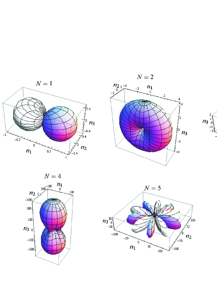
Figure 1: The Stokes moment profiles $\langle\hat{S}_{\mathbf{n}}^{N}\rangle_{N}$ for the $N$-photon NOON states with $1\leq N\leq 6$. Dark and light surfaces indicate the directions for which $\langle\hat{S}_{\mathbf{n}}^{N}\rangle_{N}$ takes positive and negative values, respectively.

5.5 NOON states

Finally, let us consider the NOON states $(|N,0\rangle+|0,N\rangle)/\sqrt{2}$, where $N>0$. These are in some sense optimal for interferometry [30]. Their Stokes moment profiles are found to be

$$\langle\hat{S}_{\mathbf{n}}^{r}\rangle_{N}^{\mathrm{NOON}}=\left\{\begin{array}[]{ll}0,&r\ \mathrm{odd,}\ N\ \mathrm{even,}\\ \displaystyle\frac{\cos(N\Phi)\sin^{N}\Theta}{4^{(N-1)/2}}\sum_{k=0}^{\frac{N-1}{2}}(N-2k)^{r}{N\choose k}(-1)^{k},&r\ \mathrm{and}\ N\ \mathrm{odd,}\\ \displaystyle\sum_{k=0}^{N}(N-2k)^{r}{N\choose k}\left[\cos^{2k}\left(\frac{\Theta}{2}\right)\sin^{2(N-k)}\left(\frac{\Theta}{2}\right)\right.&\\ \displaystyle\left.+(-1)^{k}\cos(N\Phi)\cos^{N}\left(\frac{\Theta}{2}\right)\sin^{N}\left(\frac{\Theta}{2}\right)\right],&r\ \mathrm{even.}\end{array}\right.$$ (5.51)

We note that when $r$ is even and $N$ is odd, the effect of the second term within square brackets vanishes. For each of the first six NOON states, we have plotted the Stokes moment profile $\langle\hat{S}_{\mathbf{n}}^{N}\rangle_{N}$ in figure 1. In the horizontal plane $n_{3}=0$, we have

$$\left.\langle\hat{S}_{\mathbf{n}}^{N}\rangle_{N}^{\mathrm{NOON}}\right|_{\Theta=\pi/2}=\left\{\begin{array}[]{ll}\displaystyle N!\cos(N\Phi)+2^{N/2}Q_{N/2}(N/2),&N\ \mathrm{even,}\\ &\\ \displaystyle N!\cos(N\Phi),&N\ \mathrm{odd,}\end{array}\right.$$ (5.52)

where the polynomial [31]

$$Q_{j}(n)=2^{j-2n}\sum_{k=0}^{2n}{2n\choose k}(n-k)^{2j}$$ (5.53)

satisfies $Q_{0}(n)=1$ and the recurrence relation $Q_{j+1}(n)=2n^{2}Q_{j}(n)-n(2n-1)Q_{j}(n-1)$. Hence, the de Broglie wavelength of the NOON states, which scales as $N^{-1}$ and is the reason for their superiority [32], can be seen in these measurements.

Let us now return to the pure two-photon states that satisfy $\mathbb{P}_{S}=0$. These are given in (2.7) and are found to be related to the two-photon NOON state by appropriate SU(2) transformations according to

$$|\Psi(a,\theta)\rangle=\hat{U}\left(\frac{\pi}{2}+\theta,\arccos(\sqrt{2}a),-\frac{\pi}{2}\right)\frac{|2,0\rangle+|0,2\rangle}{\sqrt{2}}.$$ (5.54)

Hence, any Stokes moment profile of the state $|\Psi(a,\theta)\rangle$ is related to the corresponding NOON profile by simple rotations. Since $\mathbf{R}_{3}(\pi/2+\theta)\cdot\mathbf{R}_{2}(\chi)\cdot\mathbf{R}_{3}(-\pi/2)=\mathbf{R}_{3}(\theta)\cdot\mathbf{R}_{1}(-\chi)$, $\langle\hat{S}_{\mathbf{n}}^{2}\rangle_{2}^{|\Psi(a,\theta)\rangle}$ is obtained from $\langle\hat{S}_{\mathbf{n}}^{2}\rangle_{2}^{\mathrm{NOON}}$ in figure 1 by applying a rotation of $-\arccos(\sqrt{2}a)$ around $\mathbf{e}_{1}$ followed by a rotation of $\theta$ around $\mathbf{e}_{3}$. Since $\langle\hat{S}_{\mathbf{n}}\rangle_{2}^{|\Psi(a,\theta)\rangle}=0$ is independent of $\mathbf{n}$, the states $|\Psi(a,\theta)\rangle$ lack first-order polarization structure. However, they do all have a second-order polarization structure.

6 Conclusions

Using expectation values of Stokes-operator products, we have developed a systematic scheme for characterizing higher-order polarization properties of two-mode quantized fields. Polarization tensors and Stokes moment profiles were introduced as two representations of the polarization information. The latter show how passive interferometry affects the moments of photon difference. This viewpoint was taken as polarization properties of different states were compared.

Other possible representations of the polarization information include central moments [4], quasi-probability distributions [33] and excitation-specific generalized coherence matrices. Complete polarization characterization requires the excitation manifolds to be addressed separately. For situations where this cannot be achieved, our characterization coincide with the one provided by Klyshko’s generalized coherence matrices [1].

Assuming ideal photon-number resolving detectors, we have shown that it is possible to efficiently collect the data through Stokes moment measurements in different directions. In an experiment, it may be more practical to use more measurement directions than the minimum required, but our method should serve as a guide. In particular, we expect the introduced moment components to be useful. Another advantage of the described method is that it treats the Stokes moments order by order. Hence, if only the first few polarization orders are of interest, it makes the measurements easier.

Since the different excitation manifolds are treated separately, losses have drastic consequences in that higher excitation manifolds then contribute to the lower ones. Furthermore, whereas linear losses often model imperfections of single-photon detectors well, photon-number resolving detectors, which are required for full polarization characterization, are more complex and may call for nonlinear modeling.

On the other hand, the separation of data into excitation manifolds and moment orders may be useful when developing methods for efficient determination of polarization characteristics. For example, one can take into account that all state projections $\hat{\varrho}_{N}$ in the different excitation manifolds must be physical states. In this way, it should be possible to develop efficient maximum likelihood methods similar to those regularly employed in common quantum tomography.

Appendix

This appendix gives a derivation of the recurrence relation (4.36), which involves central factorial numbers [27]. We let the sets of non-negative and positive integers be denoted as $\mathbb{N}_{0}$ and $\mathbb{N}_{+}$, respectively. For $x\in\mathbb{R}$, the central factorial of degree $n$ is defined by

$$x^{[n]}=\left\{\begin{array}[]{ll}1,&n=0,\\[3.61371pt] x\displaystyle\prod_{k=2-n}^{n-2}\left(x+\frac{k}{2}\right),&n\in\mathbb{N}_{+}.\end{array}\right.$$ (1.1)

The central factorial numbers of the first and second kind, $f(n,k)$ and $F(n,k)$ with $n,k\in\mathbb{N}_{0}$, respectively, are then defined through the expansions

$$x^{[n]}=\sum_{k=0}^{n}f(n,k)\,x^{k},\quad\quad\quad x^{n}=\sum_{k=0}^{n}F(n,k)\,x^{[k]}.$$ (1.2)

We note that

$$f(n,0)=F(n,0)=\delta_{n,0},$$ (1.3)

$$f(n,n)=F(n,n)=1,\quad\quad\quad n\in\mathbb{N}_{+},$$ (1.4)

where $\delta_{n,k}$ denotes the Kronecker delta. For $x\in\mathbb{R}$, we clearly have

$$x^{[2\nu]}=\prod_{j=0}^{\nu-1}(x^{2}-j^{2}),\quad\quad\quad\nu\in\mathbb{N}_{+},$$ (1.5)

$$x^{[2\nu+1]}=x\prod_{j=1}^{\nu}\left[x^{2}-\left(j-\frac{1}{2}\right)^{2}\right],\quad\quad\quad\nu\in\mathbb{N}_{0}.$$ (1.6)

Consequently, both $f(n,k)$ and $F(n,k)$ vanish if one argument is even and the other is odd. For $m\in\mathbb{N}_{0}$, $\nu\in\mathbb{N}_{+}$, and $m<\nu$, (1.2), (1.3) and (1.5) give

$$m^{[2\nu]}=\sum_{j=1}^{\nu}f(2\nu,2j)\,m^{2j}=0.$$ (1.7)

Factoring out an $m$ and making use of (1.4), we obtain

$$m^{2\nu-1}=-\sum_{j=1}^{\nu-1}f(2\nu,2j)\,m^{2j-1}.$$ (1.8)

Similarly, for $m,\nu\in\mathbb{N}_{+}$ and $m\leq\nu$, it follows from (1.6) that

$$(m-1/2)^{[2\nu+1]}=\sum_{j=0}^{\nu}f(2\nu+1,2j+1)(m-1/2)^{2j+1}=0$$ (1.9)

and

$$\sum_{j=0}^{\nu}f(2\nu+1,2j+1)(m-1/2)^{2j}=0.$$ (1.10)

Hence, for any integer $m$ satisfying $1-\nu\leq m\leq\nu$, we have

$$(m-1/2)^{2\nu}=-\sum_{j=0}^{\nu-1}f(2\nu+1,2j+1)(m-1/2)^{2j}.$$ (1.11)

Now, consider an observable $\hat{A}$ in $d$-dimensional Hilbert space with eigenvalues $\{\lambda_{j}\}_{j=1}^{d}$. In the eigenbasis, we then have $\hat{A}^{r}=\mathrm{Diag}(\lambda_{1}^{r},\lambda_{2}^{r},\ldots,\lambda_{d}^{r})$. If all eigenvalues are integers and satisfy $|\lambda_{k}|<\nu$, where $\nu\in\mathbb{N}_{+}$, (1.8) gives the recurrence relation

$$\hat{A}^{2\nu-1+\mu}=-\sum_{j=1}^{\nu-1}f(2\nu,2j)\,\hat{A}^{2j-1+\mu},$$ (1.12)

which is valid for any $\mu\in\mathbb{N}_{0}$. If all eigenvalues are half-integers and satisfy $|\lambda_{k}|\leq\nu-1/2$, where $\nu\in\mathbb{N}_{+}$, it follows from Eq (1.11) that

$$\hat{A}^{2\nu+\mu}=-\sum_{j=0}^{\nu-1}f(2\nu+1,2j+1)\,\hat{A}^{2j+\mu}.$$ (1.13)

Here, $\mu$ can take any integer value, since the inverse of $\hat{A}$ is guaranteed to exist. We note that we can apply arbitrary unitary transformations to both sides of (1.12) and (1.13), so they are valid in any basis.

Now, consider the angular momentum component $\hat{J}_{3}$ of a spin-$s$ particle. The dimension of the corresponding Hilbert space is $d=2s+1$ and the eigenvalues are $-s,-s+1,\ldots,s$. For $s\in\mathbb{N}_{+}$, the magnitudes of all eigenvalues are integers less than $s+1$ and (1.12) becomes

$$\hat{J}_{3}^{2s+1+\mu}=-\sum_{j=1}^{s}f(2s+2,2j)\,\hat{J}_{3}^{2j-1+\mu}.$$ (1.14)

If $s$ is not an integer, all eigenvalues are half-integers with magnitudes less than or equal to $s$ and (1.13) becomes

$$\hat{J}_{3}^{2s+1+\mu}=-\sum_{j=0}^{s-1/2}f(2s+2,2j+1)\,\hat{J}_{3}^{2j+\mu}.$$ (1.15)

Taking the expectation value of the corresponding recurrence relations for the Stokes operator $\hat{S}_{3}=2\hat{J}_{3}$ in excitation manifold $N=2s$, gives the desired result (4.36).

References

- [1] Klyshko D N 1997 Sov. Phys. JETP 84 1065
- [2] Müller Ch, Stoklasa B, Klimov A B, Peuntinger Ch, Gabriel Ch, Řeháček J, Hradil Z, Leuchs G, Marquardt Ch and Sánchez-Soto L L 2012 New J. Phys.14 085002
- [3] Jaeger G, Teodorescu-Frumosu M, Sergienko A, Saleh B E A and Teich M C 2003 Phys. Rev.A 67 032307
- [4] Björk G, Söderholm J, Kim Y-S, Ra Y-S, Lim H-T, Kothe C, Kim Y-H, Sánchez-Soto L L and Klimov A B 2012 Phys. Rev.A 85 053835
- [5] Raymer M G, Funk A C and McAlister D F 2000 Quantum Communication, Computing, and Measurement 2 ed Kumar P et al(New York: Plenum) p 147
- [6] Raymer M G and Funk A 2000 Phys. Rev.A 61 015801
- [7] Karassiov V P 2005 J. Russ. Laser Res. 26 484
- [8] Carozzi T, Karlsson R and Bergman J 2000 Phys. Rev.E 61 2024
- [9] Setälä T, Lindfors K, Kaivola M, Tervo J and Friberg A T 2004 Opt. Lett. 29 2587
- [10] Luis A 2005 Phys. Rev.A 71 063815
- [11] Stokes G G 1852 Trans. Cambridge Philos. Soc. 9 399
- [12] Collett E 1970 Am. J. Phys. 38 563
- [13] Schwinger J 1965 Quantum Theory of Angular Momentum ed Biedenharn L C and van Dam H (New York: Academic) p 229.
- [14] Yurke B, McCall S L and Klauder J R 1986 Phys. Rev.A 33 4033
- [15] Luis A and Sánchez-Soto L L 2000 Prog. Opt. 41 421
- [16] Björk G, Söderholm J, Sánchez-Soto L L, Klimov A B, Ghiu I, Marian P and Marian T A 2010 Opt. Commun. 283 4440
- [17] Glauber R J 1963 Phys. Rev.130 2529
- [18] Luis A and Korolkova N 2006 Phys. Rev.A 74 043817
- [19] Newton R G and Young B 1968 Ann. Phys., NY49 393
- [20] Leonhardt U 1996 Phys. Rev.A 53 2998
- [21] Weigert S 2006 Int. J. Mod. Phys. B 20 1942
- [22] Schilling U, von Zanthier J and Agarwal G S 2010 Phys. Rev.A 81 013826
- [23] Simon R and Mukunda N 1990 Phys. Lett.A 143 165
- [24] Fejes Tóth L 1965 Acta Math. Acad. Sci. Hungar. 16 437
- [25] Conway J H, Hardin R H and Sloane N J A 1996 Exp. Math. 5 139
- [26] Yu. I. Bogdanov, G. Brida, I. D. Bukeev, M. Genovese, K. S. Kravtsov, S. P. Kulik, E. V. Moreva, A. A. Soloviev, and A. P. Shurupov, Phys. Rev. A 84, 042108 (2011).
- [27] Butzer P L, Schmidt M, Stark E L and Vogt L 1989 Numer. Funct. Anal. Optimiz. 10 419
- [28] Holland M J and Burnett K 1993 Phys. Rev. Lett.71 1355
- [29] Holland M J and Burnett K 2004 Phys. Rev. Lett.92 209302
- [30] Söderholm J, Björk G, Tsegaye T and Trifonov A 1999 Phys. Rev.A 59 1788
- [31] Tuenter H J H 2002 Fibonacci Quarterly 40 175
- [32] Jacobson J, Björk G, Chuang I and Yamamoto Y 1995 Phys. Rev. Lett.74 4835
- [33] Marquardt C, Heersink J, Dong R, Chekhova M V, Klimov A B, Sánchez-Soto L L, Andersen U L and Leuchs G 2007 Phys. Rev. Lett.99 220401