On the secular behavior of dust particles in an eccentric protoplanetary disk with an embedded massive gas giant planet

Abstract

We investigate the dust velocity and spatial distribution in an eccentric protoplanetary disk under the secular gravitational perturbation of an embedded planet of about 5 Jupiter masses. We first employ the FARGO code to obtain the two-dimensional density and velocity profiles of the eccentric gas disk exterior to the gap opened up by the embedded planet in the quasi-steady state. We then apply the secular perturbation theory and incorporate the gas drag to estimate the dust velocity and density on the secular timescale. The dust-to-gas ratio of the unperturbed disk is simply assumed to be 0.01. In our fiducial disk model with the planet at 5 AU, we find that 0.01 cm- to 1 m-sized dust particles are well coupled to the gas. Consequently, the particles behave similarly to the gas and exhibit asymmetric dynamics as a result of eccentric orbits. The dust surface density is enhanced around the apocenter of the disk. However, for the case of a low-density gaseous disk (termed “transition disk” henceforth in this work) harboring the planet at 100 AU, the azimuthal distributions of dust of various sizes can deviate significantly. Overall, the asymmetric structure exhibits a phase correlation between the gas velocity fields and dust density distribution. Therefore, our study potentially provides a reality check as to whether an asymmetric disk gap detected at sub-millimeter and centimeter wavelengths is a signpost of a massive gas giant planet.

1 INTRODUCTION

Past theoretical models have demonstrated that the tidal interactions between a protoplanetary disk and an embedded giant planet clean out the region around the planet’s orbit and open up a gap (e.g. Lin & Papalouzou, 1993; Ward, 1997). Therefore, the presence of a cavity in a protoplanetary disk as revealed by dust continuum emissions has at times been postulated as a potential signpost of an embedded gas giant planet (e.g. Andrews et al., 2011, and references therein). Non-planetary explanations have also been proposed, e.g. grain growth, fast radial drift of dust, and photoevaporation (e.g. Williams & Cieza, 2011; Takeuchi et al., 2005). Evidently, a thorough understanding of the dust dynamics in a gaseous disk is essential for interpretation of such observational results.

The aerodynamic drag is a well-known interaction between gas and dust in protoplanetary disks. The presence of a radial pressure gradient causes the azimuthal gas velocity to deviate from the circular Keplerian motion, resulting in the super-Keplerian or sub-Keplerian motion. On the other hand, dust particles are unaffected by the pressure within the disk. The resulting discrepancy in the velocities gives rise to the drag force and hence a drift of the particles toward the pressure maxima (e.g. Haghighipour & Boss, 2003). This dust trapping mechanism has been previously applied to a circular disk with an embedded gas giant planet. For instance, the outer edge of the gap opened up by the planet can act as a filter to stall the radial drift of large particles in the outer disk (Rice et al., 2006). In addition, dust that is well-coupled to the gas can be temporarily trapped by the spiral density waves excited by the planet as the waves pass by (Paardekooper & Mellema, 2006).

If the planet is sufficiently massive, the disk exterior to the planet’s orbit can become moderately eccentric and start precessing on the secular timescale, depending on the disk mass and viscosity (Papaloizou et al., 2001; Kley & Dirksen, 2006). Eccentric protoplanetary disks in binary systems have also been observed in simulations as a result of the influence of a companion star (e.g. Müller & Kley, 2012). This phenomenon is reminiscent of eccentric disks in the SU Ursae Majoris systems, which have been long proposed to account for the superhump light curves (e.g. Whitehurst, 1988). The eccentricity is excited exponentially and secularly by the tidal forcing of the companion star via the 3:1 eccentric Lindblad resonance (Lubow, 1991). Goodchild & Ogilvie (2006) carried out a linear analysis for the secular perturbations with the azimuthal mode number $m=1$, and derived the so-called eccentricity equation for a gaseous disk. The equation describes the eccentric instability in terms of “eccentric modes”, with the growth and precession rates determined by given disk properties such as sound-speed and density profiles (also see Lubow, 2010). In the presence of dissipation that damps eccentricity, the slowly precessing disk finally settles into a steady state in which the eccentricity and longitude of pericenter are smooth functions of the disk radius.

In such an eccentric protoplanetary disk harboring a massive planet, the orbits of dust particles would be eccentric as well due to the gas drag. The standard gas-dust dynamics as analyzed for circular orbits (e.g. Weidenschilling, 1977; Takeuchi & Lin, 2002) is unable to yield the dust velocity and the corresponding spatial density distribution accurately. One straightforward approach for studying the dust behavior in eccentric disks is to utilize two-fluid (gas + dust) hydrodynamic simulations such as SPH codes and RODEO (Paardekooper & Mellema, 2006). In fact, because several giant planets have been discovered in close stellar binaries (binary separation $<$ 20 AU), a large body of the literature and considerable attention have been devoted to eccentric circumstellar disks in these binaries to examine the outcome of planetesimal collisions on the formation of giant planets (e.g. Paardekooper et al., 2008, and references therein). For dust particles, Fouchet et al. (2010) performed 3D SPH simulations to investigate the dynamics of dust with sizes from 0.1 mm to 1 cm in protoplanetary disks, including an eccentric disk driven by a planet of 5 Jupiter masses on a fixed circular orbit at 40 AU. After about 100 planetary orbits, they found that 1 cm-sized dust had accumulated in the strong spiral density waves just around the outer region of the gap in the disk in which the eccentricity is still evolving. At present, SPH simulations are still computationally expensive. For a small perturber like a planet, a tremendous length of time is required to reach quasi-steady states for the study of any features related to secular effects.

Therefore, for the sake of convenience, we run the FARGO code (Masset, 2000) to obtain the gas profile in a two-dimensional disk with a massive planet, and then employ the secular perturbation theory and incorporate aerodynamic drag (Paardekooper et al., 2008) to estimate the dust velocity and density that will in turn reveal the asymmetric structures inherent to an eccentric disk. The purpose of this study is to focus only on the secular behaviors of dust associated with an eccentric protoplanetary disk in the presence of a massive giant planet. Therefore, non-secular effects, such as dust-gas dynamics in the horseshoe orbit and whether dust particles can drift toward the peaks of spiral density waves in an eccentric disk (Fouchet et al., 2010), are not studied in this work.

The paper is organized as follows. In §2, we first describe the fiducial disk model for the study. We then briefly review the eccentricity equation for dust and explain our approach for solving the problem in §3. The results for the fiducial models of a protoplanetary disk and for a simple transition disk are presented in §4. We finally summarize the results and discuss the limitations of our work in §5.

2 DISK MODELS

A geometrically thin protoplanetary disk with an embedded gas giant planet is numerically simulated using the FARGO code, a two-dimensional hydrodynamic code employing an efficient modification of standard transport algorithm (Masset, 2000). Therefore, the disk pressure and density are vertically integrated quantities. The simulations are conducted in polar coordinates $(r,\phi)$ centered on the protostar. The quantities in FARGO are dimensionless. The semi-major axis of the planet $a_{p}$ is taken to be the length unit and the mass of the central protostar $M_{\star}$ is adopted as the mass unit. The time unit is obtained from $\Omega_{p}^{-1}=(a_{p}^{3}/GM_{\star})^{1/2}$ and the gravitational constant $G$ is set to 1 in FARGO.

In this study, we consider the following fiducial model with standard parameters for a locally isothermal and initially axi-symmetric gas disk (cf. Kley & Dirksen, 2006): $M_{\star}=1M_{\odot}$, $a_{p}=5$ AU, and a constant aspect ratio $H/r=0.05$, where $H$ is the vertical pressure scale height of the disk. We adopt $\nu=1\times 10^{-5}$ and $\Sigma(t=0)=1\times 10^{-4}$ to be the values of the dimensionless kinematic viscosity and initial uniform surface density, respectively. The surface density corresponds to about 35.6 g cm^-2, amounting to approximately a disk mass of $5.03\times 10^{-3}M_{\odot}$ inside $4a_{p}=20$ AU. Because all the quantities are dimensionless in FARGO, we also lower the surface density by using the larger length-scale $a_{p}=100$ AU to simulate a simplified model that resembles a “transition disk” with an embedded gas giant planet far away from its protostar. That is, with the same disk mass $5.03\times 10^{-3}M_{\odot}$ inside $4a_{p}=400$ AU, the surface density of the transition disk is about 0.09 g cm^-2. A number of gas giants have been directly imaged at $a_{p}>$ 50-100 AU around their main-sequence host stars (see The Extrasolar Planets Encyclopedia website at http://exoplanet.eu). How and when these planets lie on the current large orbits is still an open question. Some planet formation and migration models (e.g., Boss, 2011; Crida et al., 2009) suggest that these planets could have been situated on the large orbits back to their T Tauri epochs when their protoplanetary disks were still present, as is considered here for the transition disk.

To excite a noticeable disk eccentricity even for a planet on a circular orbit, we employ the initial mass ratio $q\equiv m_{p}/M_{\star}=5\times 10^{-3}$ (Kley & Dirksen, 2006). The planet mass $m_{p}$ is allowed to grow by setting the inverse of the accretion timescale to $2$ (Kley, 1999). The softening length is 0.4 times of the Hill radius of the planet. Disk self-gravity is neglected. We force the planet on a fixed circular/eccentric orbit with the apocenter located in the $\phi=0$ direction; namely, we omit the gravitational force exerted by the disk on the planet and the increments in momentum due to the mass accretion. Hence, planetary migration is not considered. Ignoring planetary migration is justified because we are interested in physical properties of an eccentric disk on secular timescales. These timescales are shorter than the typical Type II planetary migration timescale $\sim r^{2}/\nu$ (Ward, 1997), which is about a few $10^{5}$ dynamical time in our model. In the simulation, the planet initially orbits the central star counterclockwise from $\phi=0$. The computational domain in the $r$ and $\phi$ is $[0.4,4.0]\times[0,2\pi]$ with resolutions $(N_{r},N_{\phi})=(256,768)$. At both the inner and outer boundaries, we apply the non-reflecting boundary condition to avoid unphysical reflecting waves.

As for dust particles in the gaseous disk, we do not consider any dust size distributions. For the dust of a given size, we simply assume that the dust-to-gas ratio of the unperturbed disk (i.e., the disk in the absence of a planet) is 0.01. Modelling dust dynamics in the presence of a planet is described in the next session.

3 SECULAR EVOLUTION OF THE DUST

Since FARGO is a hydrodynamical code and not formulated to simulate dust particles, our approach for dust dynamics in an eccentric gaseous disk is to consider the secular evolution of the dust using the secular perturbation theory, which gives rise to the eccentricity equation. The equation describes the secular evolution of a massless particle perturbed by a companion. Given the drag force, the dust motion and surface density can then be deduced from the gas dynamics in the quasi-steady state of an eccentric disk in FARGO. However, to compute the secular evolution of dust particles, we need to filter out the short-term evolution on the orbital timescale of the planet in the gas simulation. As noted in the Introduction, the eccentric equation has been modified to include the gas drag and applied to planetesimals in a protoplanetary disk in binaries (Paardekooper et al., 2008). As per Paardekooper et al., we adopt the same eccentricity equation for solids, but with the perturbed potential in terms of the Lapalace coefficients (e.g. Tremaine, 1998; Murray & Dermott, 1999) and the gas drag appropriate for small particles (i.e. micron to meter instead of km size). The details are described as follows.

3.1 Eccentricity equation for the dust

In the subsection, we briefly review the eccentricity equation for dust particles in accordance with the the linear analysis for a gas disk by Goodchild & Ogilvie (2006), in which the variables such as velocities and density are expanded as power series in terms of $\epsilon\equiv H/r$.

Goodchild & Ogilvie (2006) considered a 2D gaseous disk with the axi-symmetric basic state allowing for a small deviation from the Keplerian circular angular velocity $\Omega_{K}$ to the accuracy of the order $\epsilon^{2}\equiv(H/r)^{2}$, due to the small background pressure gradient and orbit-averaged planet potential. After introducing the $m=1$ perturbations in the form of $\mathcal{R}[x^{\prime}(r,t)\exp(-i\phi)]$, where $\mathcal{R}$ denotes the real part, they showed that the complex eccentricity is related to the perturbed velocities at the zeroth order of $\epsilon$ (denoted by the subscript 0):

$$u_{g,0}^{\prime}=ir\Omega_{K}E_{g},\qquad v_{g,0}^{\prime}=\frac{1}{2}r\Omega_{K}E_{g},$$ (1)

where $u$ and $v$ are the radial and azimuthal velocities. $E_{g}$ is the complex eccentricity of the form $e_{g}\exp(i\varpi_{g})$ with the eccentricity, $e_{g}(r,t)$, as the amplitude, and the longitude of pericenter, $\varpi_{g}(r,t)$, as the phase angle. The subscript $g$ represents the gas to distinguish it from the subscript $d$ for dust to be used later in the paper. The above equation describes the Keplerian motion of the gas with a small eccentricity $e_{g}$, thus giving the following relation for the epicyclic motion

$$u_{g,0}^{\prime}=2iv_{g,0}^{\prime}.$$ (2)

In order to examine the secular evolution of an eccentric disk resulting from the weak companion potential and small radial pressure gradient, Goodchild & Ogilvie (2006) proceeded to the next order (i.e. at $O(\epsilon^{2})$, denoted by the subscript 2) and obtained the evolutionary equation for the complex eccentricity $E_{g}$.

Likewise, the eccentricity equation for dust particles can be obtained from the linearized equations with zero pressure. In the basic state, the dust particles in a disk are assumed to be steady, non-self-gravitating, and axi-symmetrically distributed. As such, the basic state of the dust motion reads

$$r\Omega_{d,0}=\frac{\partial\Phi_{0}}{\partial r}=r\Omega_{K},$$ (3)

$$2r\Omega_{d,0}\Omega_{d,2}=\frac{\partial\Phi_{2}}{\partial r}+{1\over t_{s}}(u_{d,2}-u_{g,2}),$$ (4)

$$u_{d,2}\Omega_{d,0}=-\frac{2r}{t_{s}}(\Omega_{d,2}-\Omega_{g,2}),$$ (5)

In the above equations, $\Phi_{0}$ is the primary potential from the central protostar, $\Omega_{d,2}$ is the dust angular velocity departure from $\Omega_{K}$ due to the orbit-averaged planet potential $\Phi_{2}$ and the radial gas drag, and $\Omega_{g,2}=(1/\Sigma_{g})(dp_{g}/dr)/(2r\Omega_{K})$ is the gas angular velocity departure from $\Omega_{K}$ due to the radial pressure gradient $dp_{g}/dr$ (Goodchild & Ogilvie, 2006). $u_{d,2}$ is the radial drift velocity arising from the gas drag characterized by the stopping time in the Epstein regime (Weidenschilling, 1977)

$$t_{s}=\frac{\rho_{d}a_{d}}{\rho_{g}\bar{v}_{th}}\qquad{\rm if}\quad a_{d}<\frac{9}{4}\lambda_{g},$$ (6)

where $a_{d}$ is the mean radius of the dust grains, $\rho_{g}$ is the gas mass density, $\rho_{d}$ is the density of a dust particle, $\bar{v}_{th}$ is the mean thermal velocity of the gas, and $\lambda_{g}$ is the mean free path of the gas. The stopping time $t_{s}$ measures the timescale for the coupling between the dust and gas in the disk. Note that in the other regimes where $\lambda_{g}$ is much smaller than $a_{d}$, the gas drag is fluid-like. Therefore both the dust and gas velocities need to be known in advance to determine the stopping time (Weidenschilling, 1977). Because the dust velocities in eccentric orbits are what we are solving for and thus not known beforehand, in this work, we therefore focus only on the dust in the Epstein regime, which can be verified in advance. As a matter of the fact, the Epstein drag is adequate for the dust sizes and disk parameters considered in this study.

Combining Equations (3)-(5), we obtain the radial drift velocity in the basic state (cf. Takeuchi & Lin, 2002)

$$u_{d,2}={\tau_{s}^{-1}u_{g,2}-\eta r\Omega_{K}-(1/\Omega_{K})(d\Phi_{2}/dr)\over\tau_{s}+\tau_{s}^{-1}},$$ (7)

where $\tau_{s}=t_{s}\Omega_{K}$ is the dimensionless stopping time and $\eta=-(c_{s}^{2}/r^{2}\Omega_{K}^{2})(d\ln p_{g}/d\ln r)$ with the isothermal sound speed $c_{s}^{2}=p_{g}/\Sigma_{g}$. For the rest of the work, we neglect $u_{g,2}$, which can be related to the slow accretion flow (Ogilvie, 2001).

For the $m=1$ secular perturbations, the dust perturbed velocity at the zeroth order can be expressed in terms of the dust eccentricity $E_{d}=e_{d}\exp(i\varpi_{d})$ as has been done for the gas component:

$$u_{d,0}^{\prime}=ir\Omega_{K}E_{d}\quad\quad v_{d,0}^{\prime}=\frac{1}{2}r\Omega_{K}E_{d},$$ (8)

which describe the epicyclic motion with the relation

$$u_{d,0}^{\prime}=2iv_{d,0}^{\prime}.$$ (9)

The eccentricity equation for dust particles can then be derived at $O(\epsilon^{2})$ (cf. Goodchild & Ogilvie, 2006), as can be found in Paardekooper et al. (2008):

$$2r\Omega_{K}\frac{\partial E_{d}}{\partial(\epsilon^{2}t)}=-i\frac{E_{d}}{r}\frac{\partial}{\partial r}\left(r^{2}\frac{\partial\Phi_{2}}{\partial r}\right)+{i\over r^{2}}{\partial\over\partial r}\left(r^{2}\Phi^{\prime}_{2}\right)-\frac{2r\Omega_{K}}{t_{s}}(E_{d}-E_{g}),$$ (10)

where the terms associated with resonant interactions and the radial drift velocity $u_{d,2}$ are ignored because we focus only on secular evolutions of eccentric orbits. The effect of the radial drift will be estimated separately by Equation (7). In the above equation, $\Phi^{\prime}_{2}$ is the $m=1$ component of the planet’s potential due to the planetary eccentricity $E_{p}$ ($=e_{p}\exp(i\varpi_{p})$). Equation (10) presents the complex form of the eccentricity equation in terms of $h\equiv e\sin\varpi$ and $k\equiv e\cos\varpi$ derived from the Lagrange’s planetary equation in the secular perturbation theory (e.g., Tremaine, 1998; Murray & Dermott, 1999; Marzari & Scholl, 2000). Hence, we can express $\Phi_{2}$ and $\Phi^{\prime}_{2}$ in terms of the Lapalace coefficients, and simplify Equation (10) to

$$\frac{\partial E_{d}}{\partial(\epsilon^{2}t)}=i\frac{E_{d}}{t_{prec,d}}+i\frac{E_{p}}{t_{f}}-\frac{E_{d}-E_{g}}{t_{s}},$$ (11)

where $t_{prec,d}$ and $t_{f}$ are given by (e.g. Tremaine, 1998; Murray & Dermott, 1999)

$$t_{prec,d} = \frac{4}{q}\left(\frac{r}{a_{p}}\right)\left(\frac{1}{b_{3/2}^{(1)}\left(\frac{a_{p}}{r}\right)}\right)\frac{1}{\Omega_{K}},$$ (12)

$$t_{f} = \frac{4}{q}\left(\frac{r}{a_{p}}\right)\left(\frac{1}{b_{3/2}^{(2)}\left(\frac{a_{p}}{r}\right)}\right)\frac{1}{\Omega_{K}},$$ (13)

and the Laplace coefficients $b_{3/2}^{(1)}$ and $b_{3/2}^{(2)}$ can be computed numerically by Carlson’s algorithm (Press et al., 1992). $t_{prec,d}$ is the precession timescale of a free particle on an eccentric orbit, whereas $t_{f}$ is related to the forced eccentricity in the secular perturbation theory (see below).

We consider the steady-state situation for dust particles. The eccentricity equation (11) is then reduced to (cf. Paardekooper et al., 2008)

$$E_{d}=E_{f}{1\over\sqrt{1+1/\tau_{s,sec}^{2}}}\exp[i\arctan(-(1/\tau_{s,sec})]+E_{g}{1\over\sqrt{1+\tau_{s,sec}^{2}}}\exp[i\arctan(\tau_{s,sec})].$$ (15)

where

$$\tau_{s,sec} \equiv \frac{t_{s}}{t_{prec,d}},$$ (16)

$$E_{f} \equiv \frac{t_{prec,d}}{t_{f}}E_{p}.$$ (17)

In the above equations, $E_{f}$ is the forced eccentricity from the secular perturbation theory, with the amplitude $e_{f}<e_{p}$. In addition, we define the dimensionless “secular” stopping time $\tau_{s,sec}$, the ratio of the stopping time to the precession timescale of a free particle. In analogy to the definition of $\tau_{s}$, $\tau_{s,sec}$ measures the degree of the coupling between a dust and the gas in the secular evolution.

In the case of the planet on a circular orbit, $E_{f}=0$ and Equation (15) implies that $\varpi_{d}$ lags $\varpi_{g}$ by the phase angle $=\arctan(\tau_{s,sec})$. When $\tau_{s,sec}\ll 1$, $E_{d}\approx E_{g}$ and therefore particles are well-coupled to the gas on the secular timescale. In this case, the dust orbit is almost identical to the gas eccentric orbit. When $\tau_{s,sec}>1$, the particles are weakly coupled to the gas, and the drag force wields no or little effects. Thus, the dust particles are in near-Keplerian circular motion, provided that the planetary eccentricity is zero. Nevertheless, all dust orbits with different eccentricities and pericenters precess with the gas at the same rate in a steady state.

On the other hand, for eccentric planet orbits ($e_{p}\neq 0$), $E_{f}$ in Equation (15) may affect $E_{d}$ significantly depending on $\tau_{s,sec}$. In the regime where $\tau_{s,sec}\ll 1$, the dust is strongly coupled to the gas and thus $E_{d}\approx E_{g}$. In the other regime where $\tau_{s,sec}>1$, the gas drag does not dominate the dust motion but plays a role secondary to the planet’s potential in providing the free eccentricity to dust particles in the steady state (Paardekooper et al., 2008). When $\tau_{s,sec}|E_{f}|>|E_{g}|$ for a given dust size, Equation (15) describes pericenter alignment of the dust with a libration rate equal to the precession rate of the gas disk $\dot{\varpi}_{g}$. If $\tau_{s,sec}$ is moderately larger than 1 as well, the alignment is close to the planet’s pericenter.

3.2 Calculations of dust velocity and density to the zeroth order

Once $E_{d}$ is known from Equation (15), the secular solution of the dust velocity as a function of $r$ and $\phi$ can be obtained as follows

$$u_{d} = \mathcal{R}(u^{\prime}_{d,0}e^{-i\phi})+O(\epsilon^{2})$$ (18)

$$= r\Omega_{K}[\mathcal{R}(E_{d})\sin\phi-\mathcal{I}(E_{d})\cos\phi]+O(\epsilon^{2}),$$

$$v_{d} = r\Omega_{K}+\mathcal{R}(v^{\prime}_{d,0}e^{-i\phi})+O(\epsilon^{2})$$ (19)

$$= r\Omega_{K}+\frac{1}{2}r\Omega_{K}[\mathcal{R}(E_{d})\cos\phi+\mathcal{I}(E_{d})\sin\phi]+O(\epsilon^{2}),$$

where $\mathcal{R}$ and $\mathcal{I}$ denote the real and imaginary parts, respectively.

To compute $E_{d}$ in Equation (15), we need the complex gas eccentricity $E_{g}=e_{g}\exp(i\varpi_{g})$. The values of $e_{g}$ and $\varpi_{g}$ can be derived from the velocity fields in the simulation. Time averaging is first performed to reveal the secular $m=1$ results associated with the eccentric disk. We then calculate the eccentricity from the eccentricity vector and compute the longitude of pericenter from $\phi=f+\varpi$, where $\phi$ is the true longitude and $f$ is the true anomaly. In the FARGO code, the direction of reference points to $\phi=0$ and for the case of $e_{p}\neq 0$, $\varpi_{p}=\pi$ (i.e. $E_{p}=-e_{p}$). To evaluate the stopping time, we employ the mean free path (Rice et al., 2006)

$$\lambda_{g}=\frac{4\times 10^{-9}}{\rho_{g}}\text{ cm},$$ (20)

where $\rho_{g}=\Sigma_{g}/(\sqrt{2}\pi H)$, $\Sigma_{g}$ is the gas surface density, and $\rho_{d}=1.25\text{ g cm${}^{-3}$}$ (Takeuchi & Lin, 2002).

The non-axisymmetric dust spatial distribution associated with the secular evolution in an eccentric disk is of great interest because it can be observed by mapping the dust continuum emissions from a disk. The perturbed dust surface density to the zeroth order is estimated from the $m=1$ linearized continuity equation (Ogilvie, 2001):

$$\Sigma_{d,0}^{\prime}=r\frac{\partial}{\partial r}(\Sigma_{d,0}E_{d}).$$ (21)

Consequently, the total dust surface density in the eccentric disk is given by

$$\Sigma_{d}=\Sigma_{d,0}+\mathcal{R}(\Sigma_{d,0}^{\prime}e^{-i\phi})+O(\epsilon^{2}).$$ (22)

To obtain the zeroth-order basic state of dust density $\Sigma_{d,0}$ in the above equation, we first take the azimuthal average of the gas density in the simulation as the zeroth-order basic state, and assume the dust-to-gas ratio to be $0.01$ everywhere. Since we omit the size distribution of the particles, the computed dust density does not represent the true magnitude.

4 RESULTS

We present the results for two different planetary eccentricities, $e_{p}=0$ and 0.1, for a disk of standard parameters (a protoplanetary disk) and for a low-density disk (a transition disk). The general gas dynamics in the dimensionless units for our fiducial model is shown and described first. The physical units are then considered to present the results for the dust velocities and the resulting dust surface densities in both the protoplanetary and transition disks.

4.1 General gas dynamics

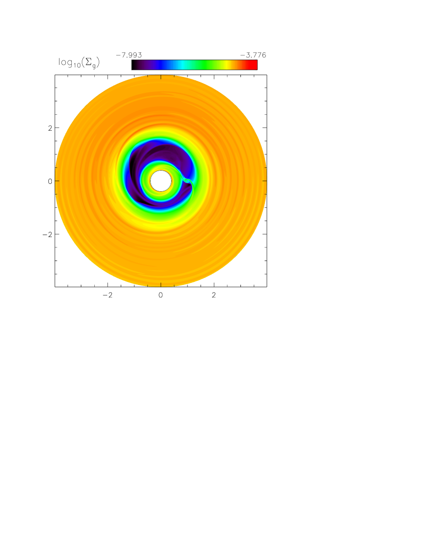
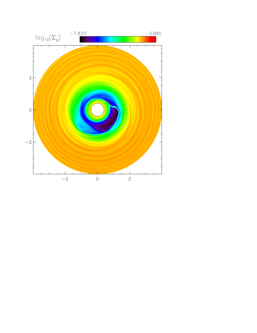
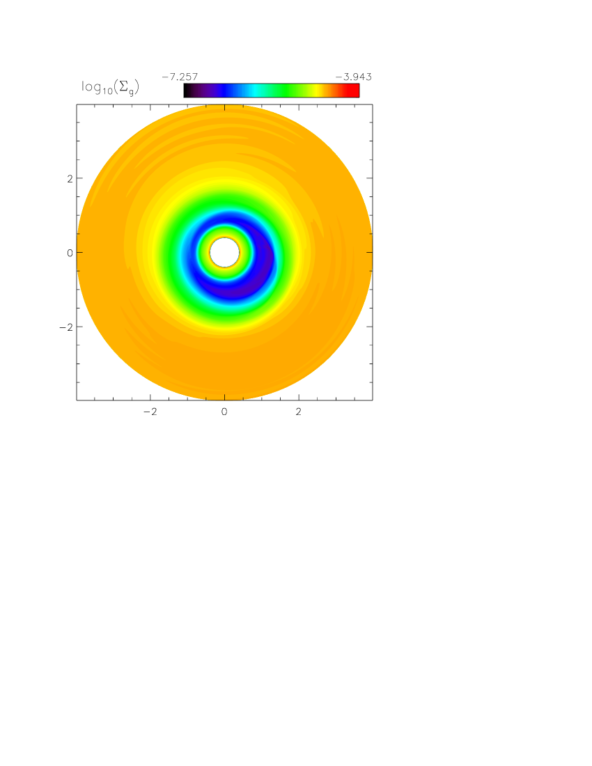
Figure 1: The quasi-steady maps of gas surface densities in the dimensionless units for $e_{p}=0$ (left panels) and $e_{p}=0.1$ (right panels). The top panels show the snap shots at $t=3000$ and the gas surface densities in the bottom panels are the time-averaged values of those shown in the top panels to erase most of the short-period spiral features.

We present the results for the cases of $e_{p}=0$ and $e_{p}=0.1$ at $t=3000$ orbits to illustrate the typical gas dynamics in a quasi-steady state. At this time, the planetary mass increases by about 6.8% in the $e_{p}=0$ case and by about 16% in the $e_{p}=0.1$ case. The gas surface density are shown in the top panels of Figure 1, where the planet lies at $(r,\phi)=(1,0)$ for $e_{p}=0$ and at (1.1,0) for $e_{p}=0.1$. We plot the densities color-coded on the logarithmic scale to clearly display the structure of the gap. The gas disk exterior to the planetary orbit apparently becomes eccentric, especially in the gap region. Furthermore, the exterior disk precesses slowly at the rate of $\dot{\varpi}_{g}\approx-(1/399)\Omega_{p}$ for $e_{p}=0$ and $-(1/152.8)\Omega_{p}$ for $e_{p}=0.1$. The absolute values of $\dot{\varpi}_{g}$ are much smaller than $\Omega_{p}$ indicative of the secular behavior of the eccentric mode with $m=1$. The negative value implies regression, i.e. retrograde precession. According to the linear theory by Goodchild & Ogilvie (2006) and the simulation by Kley et al. (2008), the disk regression in our simulation is probably due to the fact that the disk global pressure gradient plays a more important role than the planetary potential in contributing to $\dot{\varpi}_{g}$. In contrast, the disk interior to the planetary orbit remains almost circular.

Besides the eccentric mode, the planetary potential also induces the short-period features manifested by tightly wound spiral density waves in the top panels of Figure 1. The interior disk is dominated by the $m=2$ waves, as has been typically seen in the simulations for a circular disk (e.g. Kley, 1999), whereas the exterior disk is dominated by the $m=1$ waves that are distorted by the eccentric shape of the disk. These short-period features are associated with the predominant modes with pattern speeds equal to $\Omega_{p}$ and $\Omega_{p}/2$ (Lubow, 1991; Kley & Dirksen, 2006). As a result, the gas motions associated with the density waves are periodic and would be cancelled out when averaged over one orbital cycle of the planet to reveal secular features. Because of the disk regression, the time averaging is performed in the non-rotating frame for each grid point over the period of $0.9975\times 2\pi/\Omega_{p}$ for $e_{p}=0$ and $0.9935\times 2\pi/\Omega_{p}$ for $e_{p}=0.1$, instead of one planetary orbital period $2\pi/\Omega_{p}$.

The resulting time-averaged gas density is presented in the bottom panels of Figure 1. At this point, the short-period features due to the tightly wound spiral density waves are almost removed, albeit not completely. It is likely due to the quasi-steady results. The color-coded density maps suggest that the gap of the disk with the planet on an eccentric orbit appears wider but shallower than that with the planet on a circular orbit. We plot the azimuthal average of the gas densities in Figure 2, which confirms the gap shape in relation to the planetary eccentricity. Note that the disk starts to become tidally truncated roughly at the 3:1 eccentric outer and inner Lindblad resonances at $r\approx 2.08$ and at $r\approx 0.48$, respectively. Hereafter in the paper, the gap is referred to the region from $r\approx 0.5$ to 2.

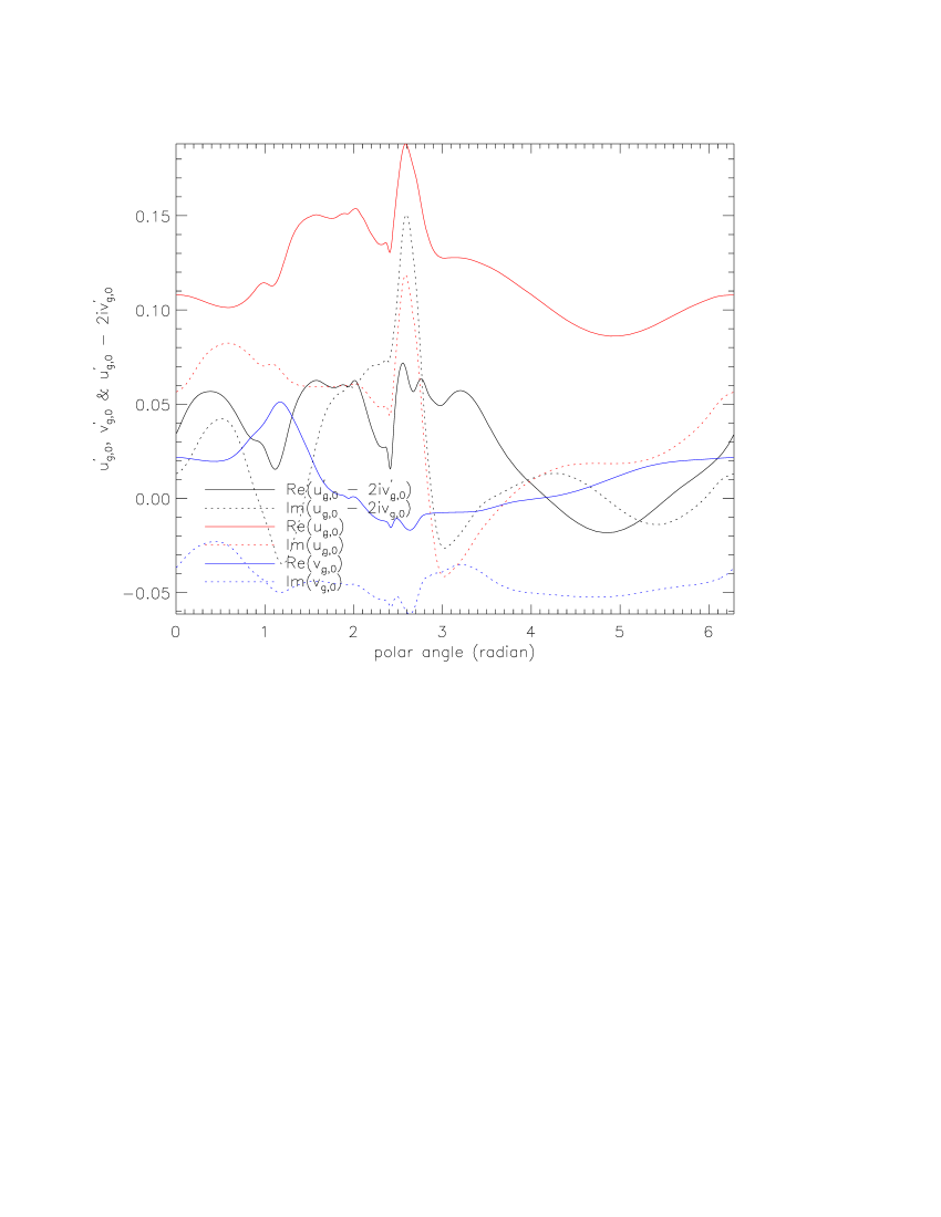
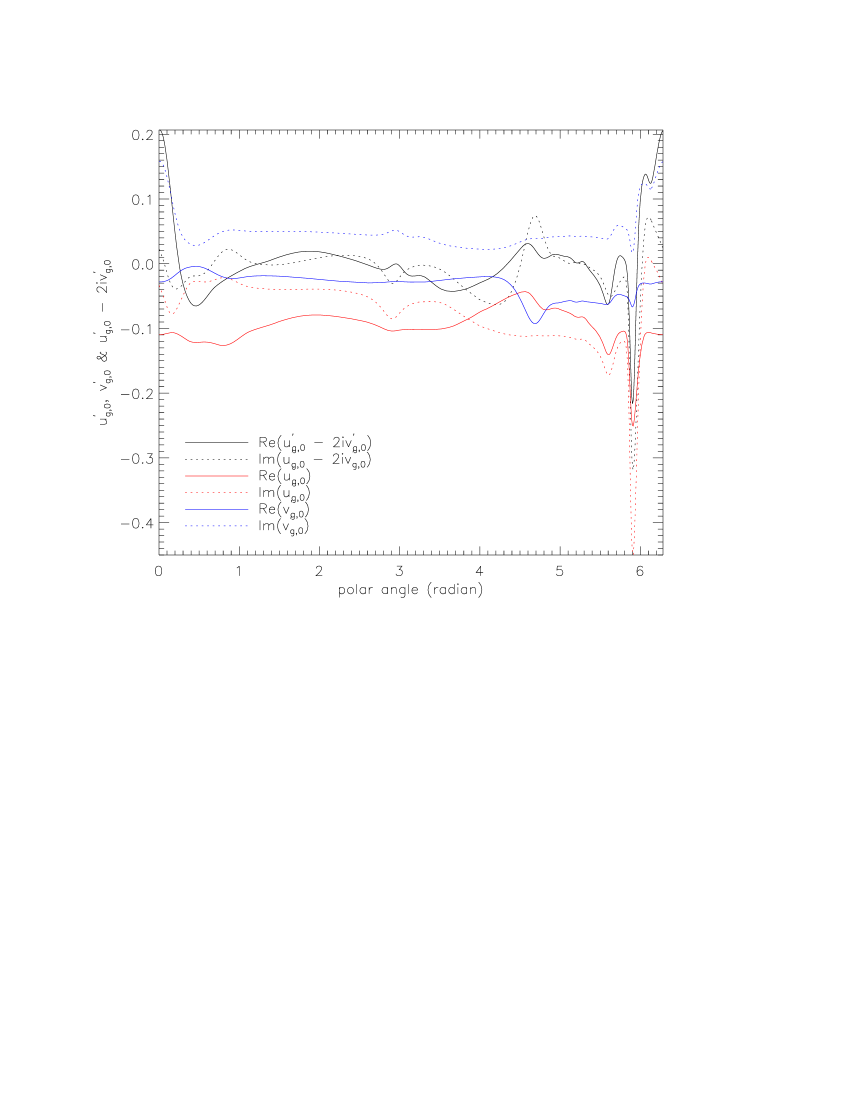
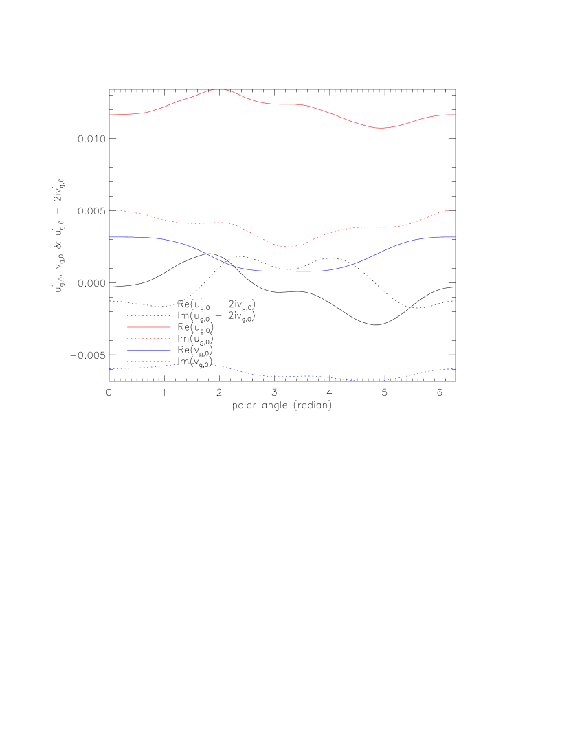
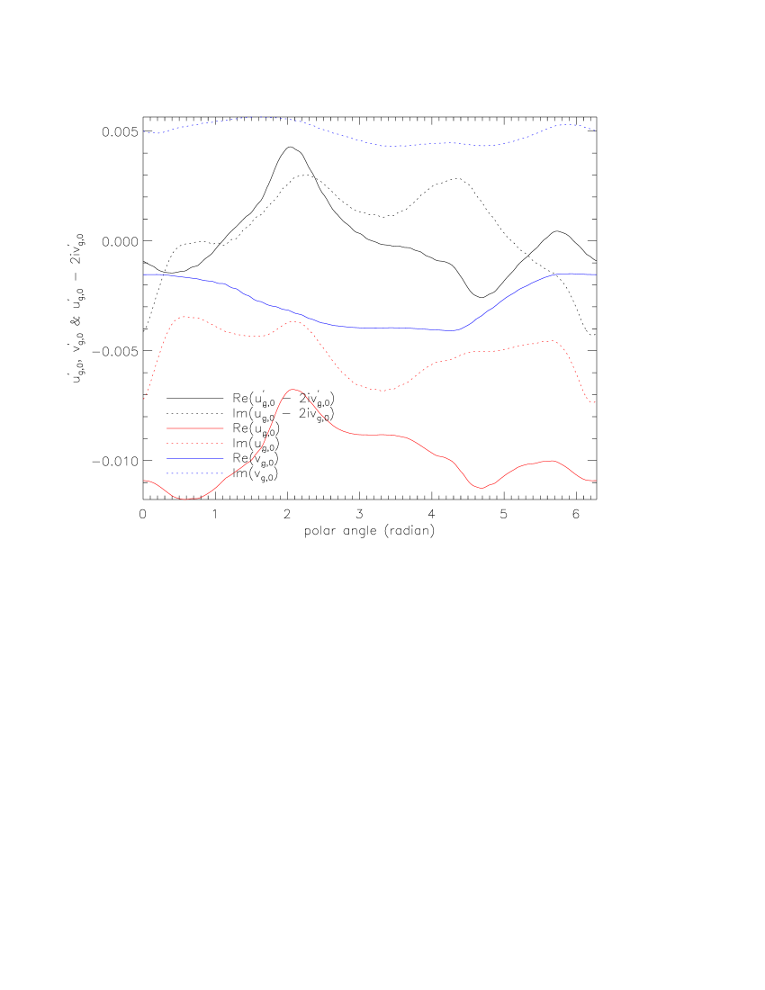
Figure 3: The results of verifying whether the relation $u_{g,0}^{\prime}=2iv_{g,0}^{\prime}$ is satisfied at $r=1.5$ (top), $r=2$ (middle) and $r=3$ (bottom) for the cases of $e_{p}=0$ (left) and 0.1 (right). The real and imaginary parts are denoted by solid and dotted lines. The red lines represent the values of $u_{g,0}^{\prime}$ and the blue lines are those of $v_{g,0}^{\prime}$. The values of the relation are shown in black.

The time-averaged density distribution of the exterior disk is predominated by the $m=1$ azimuthal distribution, a feature associated with the eccentric mode. However, the time-averaged gas flows inside the gap from $r\approx 0.5$ to 2 is more complicated than the eccentric motions. We examine whether Equation (2) is satisfied by an eccentric disk at 3 different disk radii ($r=$ 1.5, 2, and 3) for the time-averaged flow. This is illustrated in Figure 3 for the $e_{p}=0$ (left panels) and $e_{p}=0.1$ (right panels) cases. For $r=1.5$, the black curves show that Equation (2) is poorly satisfied, likely a result of the irregular horseshoe orbit associated with an eccentric disk and the non-linear effects due to the strong planetary potential. Secular effects should be predominant away from the co-orbital region within the gap. Indeed, farther away from the planet, all the curves become much smoother as shown for $r=2$ and 3, indicating that the eccentric mode has become predominant. In view of the complicated gas motion inside the gap, for the rest of study, we focus only on the secular results outside $r=2$ where the azimuthal average of gas density $\Sigma_{g,0}>9\times 10^{-5}$ for $e_{p}=0$ and $>5\times 10^{-5}$ for $e_{p}=0.1$ as indicated in Figure 2.

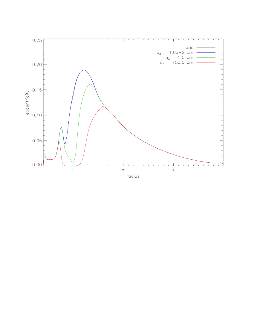
Figure 5: Azimuthally averaged eccentricities of gas and dust particles of various sizes in the cases of $e_{p}=0$ (left panel) and $e_{p}=0.1$ (right panel). The forced eccentricity $e_{f}=|E_{f}|$ is also plotted for the $e_{p}=0.1$ case.

The departures of the gas velocity from the Keplerian circular motion (i.e. the perturbed velocity) for the time-averaged disk are displayed in Figure 4. Both the perturbed radial velocity $u^{\prime}_{g}=u_{g}$ and the perturbed azimuthal velocity $v^{\prime}_{g}=v_{g}-r\Omega_{K}$ exhibit $m=1$ azimuthal profiles, as to be expected from the bottom panels of Figure 1. Moreover, Figure 4 shows that the phase difference between $u_{g}$ and $v_{g}-r\Omega_{K}$ is $90^{\circ}$, in agreement with the epicyclic motion for an eccentric disk described by Equation (2). Namely, $u_{g}\approx u^{\prime}_{g,0}$ and $v_{g}-r\Omega_{K}\approx v^{\prime}_{g,0}$ as has been verified in Figure 3. According to the color coding, the perturbed velocities are larger around the outskirts of the gap region (i.e. $r\gtrsim 2$) and become progressively smaller toward the edge of the simulated disk, implying that the disk eccentricity decreases with the radius. This is confirmed by the azimuthally averaged eccentricity profile of the gas disk as shown in the solid lines in Figure 5, which is similar to the eccentricity profile shown in Kley & Dirksen (2006). Note that the eccentricity profile is calculated and plotted all the way into the gap and inner disk region in order to facilitate comparison with the results from Kley & Dirksen (2006). The fast decay of the eccentricity profile with radius beyond the planet’s orbit seems to be in agreement with that of a confined eccentric mode in the linear secular theory by Goodchild & Ogilvie (2006), even though an eccentric disk is not a good description of a horseshoe flow within the gap (see Figure 3). In the exterior disk, the magnitudes of the epicyclic velocities and the corresponding disk eccentricities are similar between the $e_{p}=0$ and 0.1 cases.

4.2 Protoplanetary Disks

Now we turn to the specific case for the protoplanetary disk with $a_{p}=5$ AU. The values of the gas velocities in the eccentric disk can be obtained by multiplying the velocities in Figure 4 by $1.33\times 10^{6}$ cm s^-1.

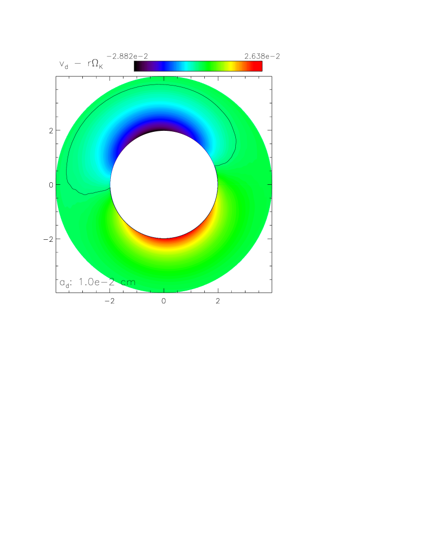
Figure 6: Radial (top panels) and azimuthal (bottom panels) dust velocities departure from the Keplerian circular velocity for the $e_{p}=0$ case. The left panels show the results for size of $1\times 10^{-2}$ cm and the right panels show the results for $1$ m. The black lines are the zero contours. The unit of the velocity is about $1.33\times 10^{6}$ cm s^-1.

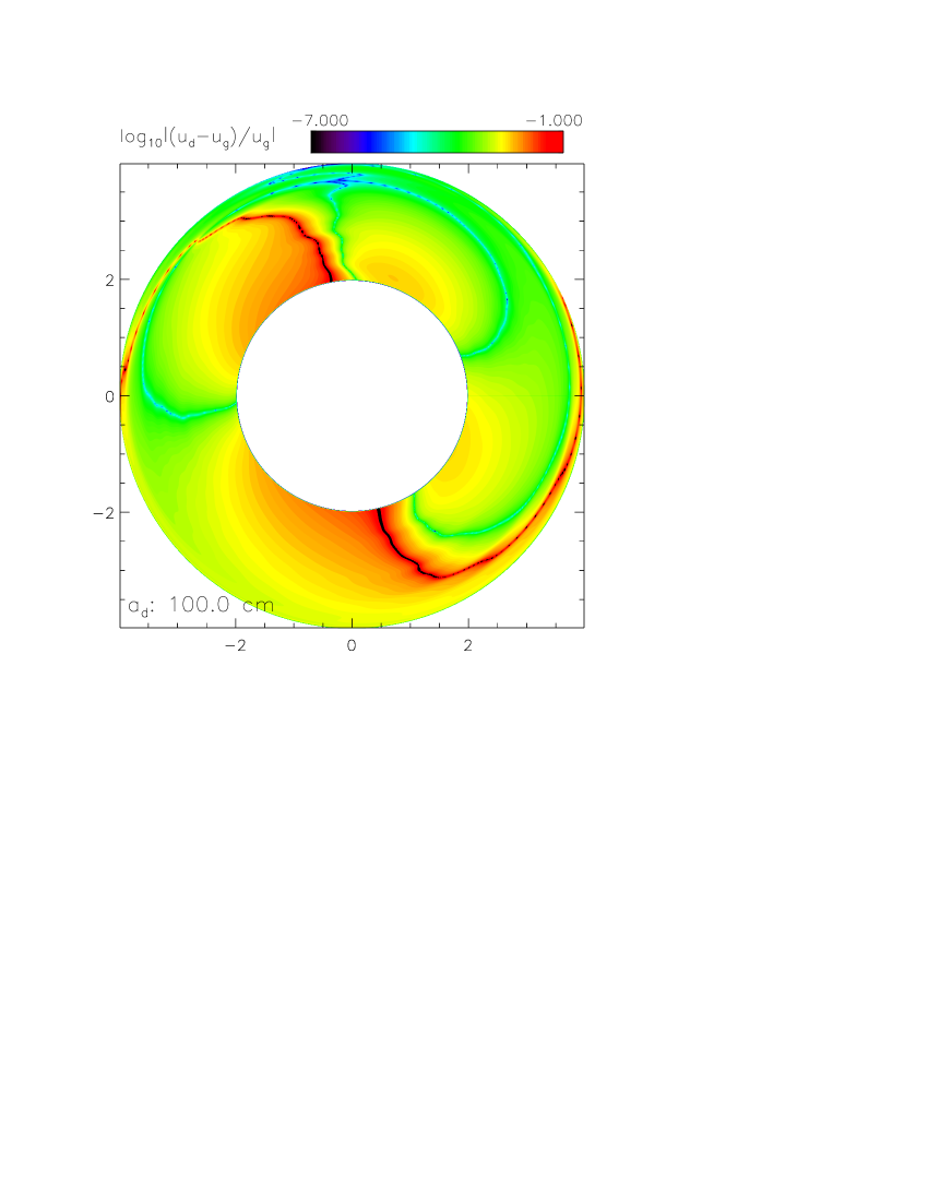
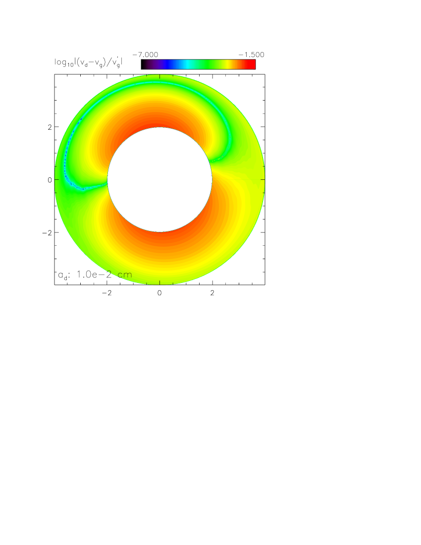
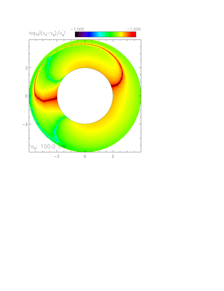
Figure 7: Absolute values of the fractional differences between the gas velocities shown in the left panels of Figure 4 and the dust velocities shown in Figure 6 for the $e_{p}=0$ case. The radial velocity difference is plotted in the top panels and azimuthal velocity difference is illustrated in the bottom panels. The left panels show the results for size of $1\times 10^{-2}$ cm and the right panels show the results for $1$ m. The fractional differences can become large ($\gtrsim 1$) in the regions where $u_{g}$ or $v^{\prime}_{g}$ is close to zero and thus we limit the top scale to show the value on the entire disk clearly. In the right panels for meter-sized particles, the narrow black curves indicate the regions where the fractional differences are too large and thus out of scale.

Figure 6 illustrates the perturbed velocities for the particles with the size of $1\times 10^{-2}$ cm and $100$ cm in the $e_{p}=0$ case. The figure shows the $m=1$ distribution due to the eccentric exterior disk. The results for the two particle sizes are indistinguishable because $\tau_{s,sec}\ll 1$ in Equation (15). More specifically, $\tau_{s,sec}$ is $1.67\times 10^{-(6-7)}$ for the 0.01 cm-sized dust particles and $1.67\times 10^{-(2-3)}$ for the 100 cm-sized dust particles. Hence the particles smaller than one meter are well coupled to the gas by the strong gas drag. It is further validated in Figure 7, which shows small fractional differences ($\ll 1$) between the dust velocities in Figure 6 and the gas velocities in the left panels of Figure 4. Similar results for strong dust-gas coupling are also found for the $e_{p}=0.1$ case; the perturbed dust velocities (not shown) are almost identical to those displayed in the right panels of Figures 4 and the values of $\tau_{s,sec}$ are on the same order as those for the $e_{p}=0$ case. Figure 5 shows that in both the $e_{p}=0$ and $e_{p}=0.1$ cases, the eccentricity profile of the gas disk and that of the well-coupled dust coincide and decrease outwards from $e=0.08$ at $r=2$. Consequently, as in the case for the gas disk, the $m=1$ velocity fields for dust particles are more prominent in the region around the outer edge of the gap where the radial velocity associated with the eccentric orbit is up to about 744.8 m/s. The forced eccentricity $e_{f}=|E_{f}|$ is also plotted in the right panel of Figure 5 for comparison with the case where $e_{p}$ is non-zero. It is apparent that in the region that our study focuses on (i.e. $r\geq 2$), the dust particles with size smaller than 1 m are so well-coupled to the gas that their eccentricity profiles are clearly distinct from $e_{f}$, i.e. $E_{d}\approx E_{g}$ for $\tau_{s,sec}\ll 1$ from Equation (15). Consequently, all particles smaller than 1 m regress with the gas disk at the same rate in the steady state.

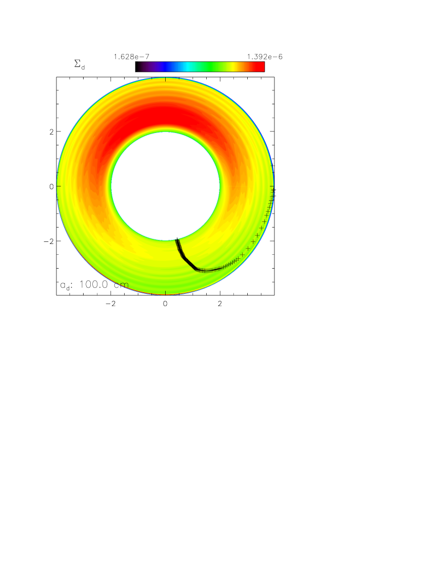
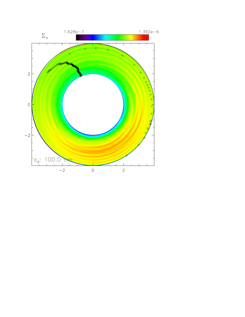
Figure 8: The spatial distribution of the dust surface density of various grain sizes for the $e_{p}=0$ (left panels) and $e_{p}=0.1$ cases (right panels). The length unit is $5$ AU and the mass unit is 1 $M_{\odot}$. Hence, the unit of the surface density is about $3.56\times 10^{-1}$ g cm^-2. The plus signs in the plots mark the azimuthally averaged longitude of pericenter for dust $\varpi_{d,ave}$.

The time-averaged surface densities for the 0.01 cm- and 100 cm-sized particles are shown in Figure 8. The $e_{p}=0$ case is plotted in the left panels and the $e_{p}=0.1$ case is presented in the right panels. By comparison with the bottom panels of Figure 1, we can see that the $m=1$ distributions of the dust and gas density look similar. In fact, a more careful comparison indicates that the dust density distributions for all the cases are almost identical to the gas density distribution, as one would expect for well-coupled dust particles. The dust distributions are asymmetric in the exterior eccentric disk. The location of the azimuthally averaged longitude of pericenter $\varpi_{d,ave}$ is illustrated on the disk by the plus signs, which are almost $180^{\circ}$ apart from the dust density peak as shown in the figure. It can be easily understood by inspecting Equations (21) & (22). The perturbed dust density $\Sigma^{\prime}_{d,0}$ is approximately equal to $\Sigma_{d,0}E_{d}(d\ln e_{d}/d\ln r$), where $d\varpi_{d}/dr$ has been neglected, as can be validated from Figure 8. Since $d\ln e_{d}/d\ln r<0$ from Figure 5, $\Sigma^{\prime}_{d,0}\propto-E_{d}.$ Hence the phase difference between $\Sigma^{\prime}_{d,0}$ and $E_{d}$ is $180^{\circ}$, implying that the density peak lies more or less at the location of the apocenter of the disk. The result can be found quite intuitive by inspecting the divergence of the dust velocity fields shown in Figure 6. As the dust particles move toward the apocenter (pericenter), the divergence of the velocity fields is negative (positive) and thus the streamlines are being compressed (rarefied), therefore finally reaching the maximum (minimum) surface density at the apocenter (pericenter).

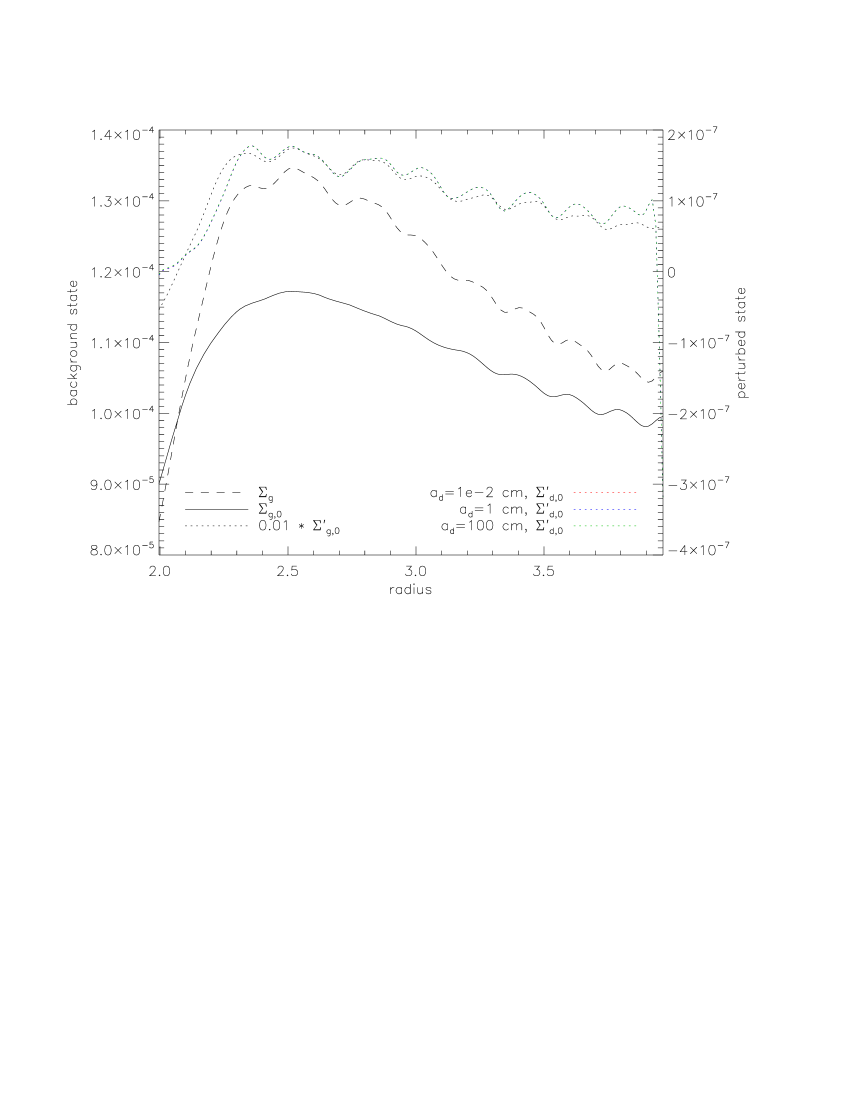
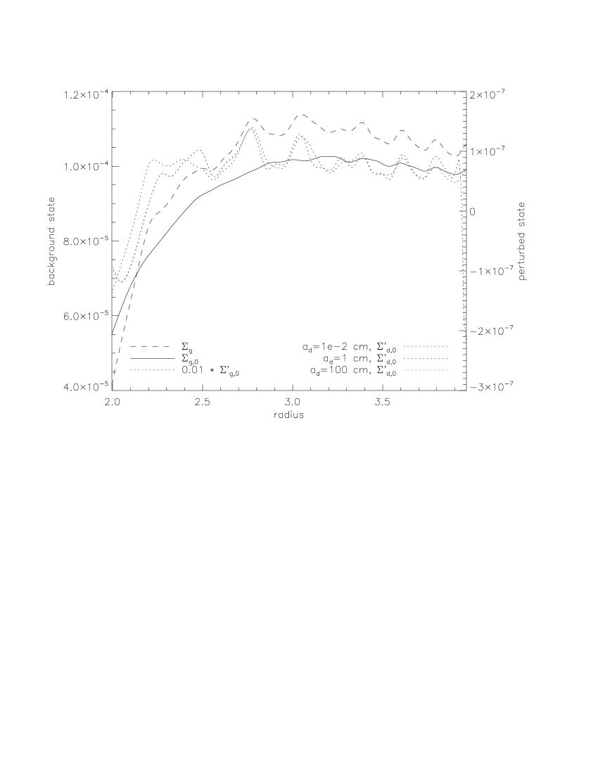
Figure 9: The density radial profiles at $\phi=110^{\circ}$ for the $e_{p}=0$ case (left panel) and at $\phi=300^{\circ}$ for the $e_{p}=0.1$ case (right panel). $\Sigma_{g}$ is the gas density after time averaging. $\Sigma_{g,0}$ is the azimuthal average of $\Sigma_{g}$ and therefore is the background gas density. $\Sigma_{g,0}^{\prime}$ and $\Sigma_{d,0}^{\prime}$ are the perturbed gas and dust densities, respectively. The scales for the background and perturbed values are shown on the left and right sides of each panel, respectively. Note that the wave-like features on the perturbed density profiles are the residuals of the short-period structures after time averaging. Nevertheless, they are small enough for estimating the order of magnitude of the secular density value $\Sigma_{d,0}^{\prime}$.

We see from Figure 8 that after time averaging, there still exist residual density fluctuations associated with short-period density waves, as has already been noted for Figure 1 in the paper. Nevertheless, the residual density is small enough to reveal the density profiles corresponding to the secular $m=1$ eccentric disk. It is illustrated in Figure 9, which shows the background and perturbed density profiles along the polar direction where the time-averaged dust density $\Sigma^{\prime}_{d,0}$ is at its maximum. Corresponding to $\phi=110^{\circ}$ and $300^{\circ}$ respectively for the $e_{p}=0$ and $0.1$ cases in Figure 8, Figure 9 shows that although the residual waves are present, they are small enough for the identification of the secular value of $\Sigma^{\prime}_{d,0}$ from order-of-magnitude estimates. In terms of the dimensionless units, the background dust surface density $\Sigma_{d,0}$ is about $10^{-6}$. Figure 9 indicates that the excess/deficit of the dust density $\Sigma^{\prime}_{d,0}$ associated with the $m=1$ eccentric disk is about $10^{-7}$ (i.e. $\sim 0.1\Sigma_{d,0}$). Other than the secular density perturbations of dust due to the eccentric disk, we also estimate the local density perturbations of dust due to the tightly wound gas density waves for comparison. The perturbed gas density of the spiral density waves $\Sigma^{\prime}_{g,wave}$ is about $0.1\Sigma_{g,0}$ from the hydrodynamical simulation. Given the dust-to-gas ratio 0.01, the perturbed dust density associated with the density waves is then given by $0.01\Sigma^{\prime}_{g,wave}\sim 0.001\Sigma_{g,0}=0.1\Sigma_{d,0}$, which is about the same order as the secular density perturbations of dust $\Sigma^{\prime}_{d,0}$.

The above 2D dust analysis does not take into account the background radial drift with the speed described by $u_{d,2}$ in Equation (7). The importance of the radial drift can be evaluated by comparing the radial drift timescale $t_{drift}\sim r/u_{d,2}$ to the precession time $t_{prec}=2\pi(399/\Omega_{p})$ for $e_{p}=0$ and $2\pi(152.8/\Omega_{p})$ for $e_{p}=0.1$. Using Equation (7) with $u_{g,2}=0$ and $d\ln p_{g}/d\ln r=-5/4$ in our isothermal model, we find that $t_{prec}/t_{drift}$ is about $5\times 10^{-(3-4)}$ for 0.01 cm-sized dust particles and about 0.3-0.5 for 100 cm-sized particles. Meter-sized particles drift inwards relatively fast at a rate almost comparable to the precession rate because the dimensionless stopping time $\tau_{s}\sim 1$ for meter-sized particles (Weidenschilling, 1977) in contrast to $\tau_{s}\ll 1$ for 0.01 cm-sized dust particles. The values of $t_{prec}/t_{drift}$ imply that the particles smaller than 1 m slowly drift inwards to the adjacent eccentric orbit after a number of orbital regressions in the protoplanetary disk.

4.3 Transition Disks

To study the dust behavior in a “transition” disk defined simply by a disk with a low gas density, we apply $a_{p}=100$ AU as the new length unit to the dimensionless simulation results presented in §4.1. The initial gas density is then reduced to about $8.89\times 10^{-2}$ g cm^-2. The resulting disk accretion rate $\sim\nu\Sigma$ is diminished by a factor of 90 or so. The drag force is weakened accordingly due to the low gas density. Hence, the spatial distribution of the dust particles with different sizes would be significantly different.

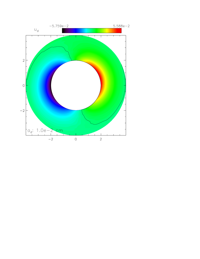
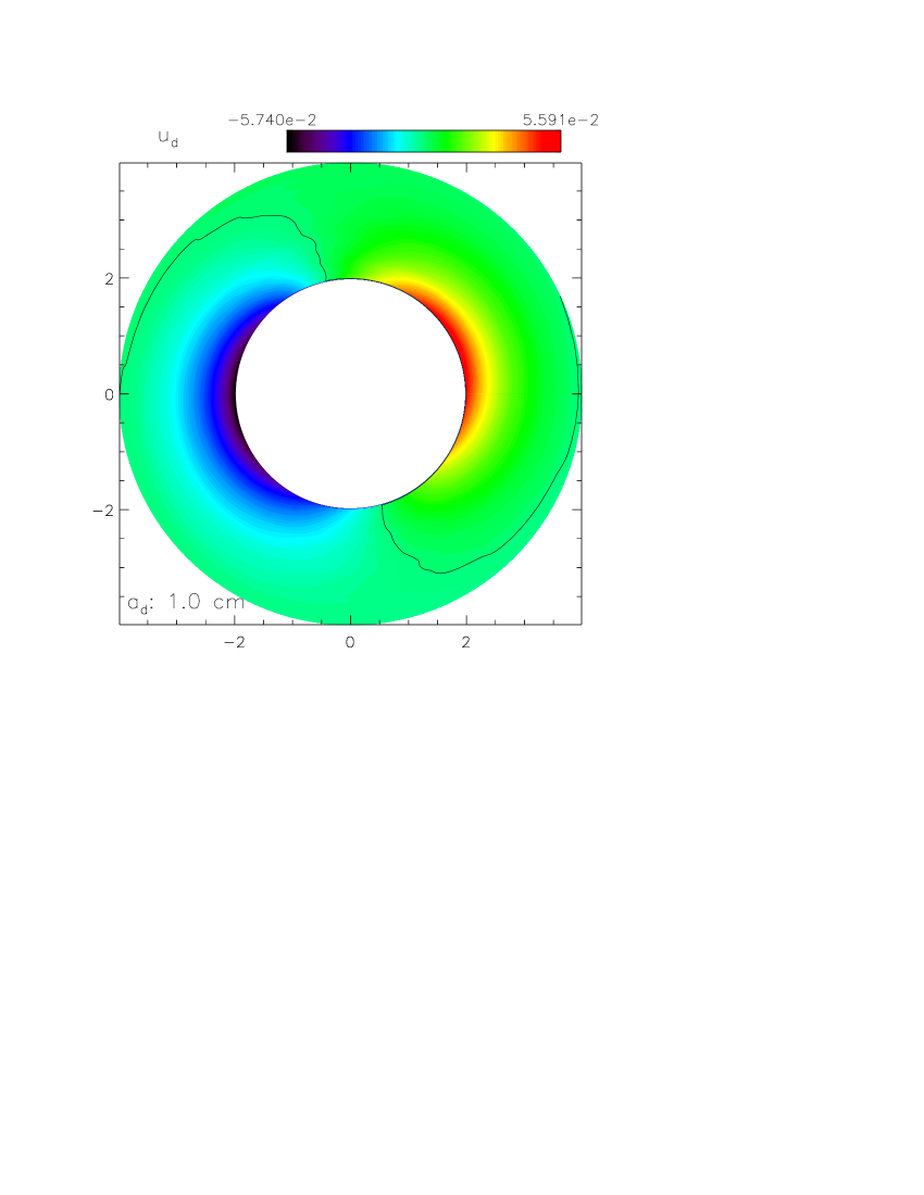
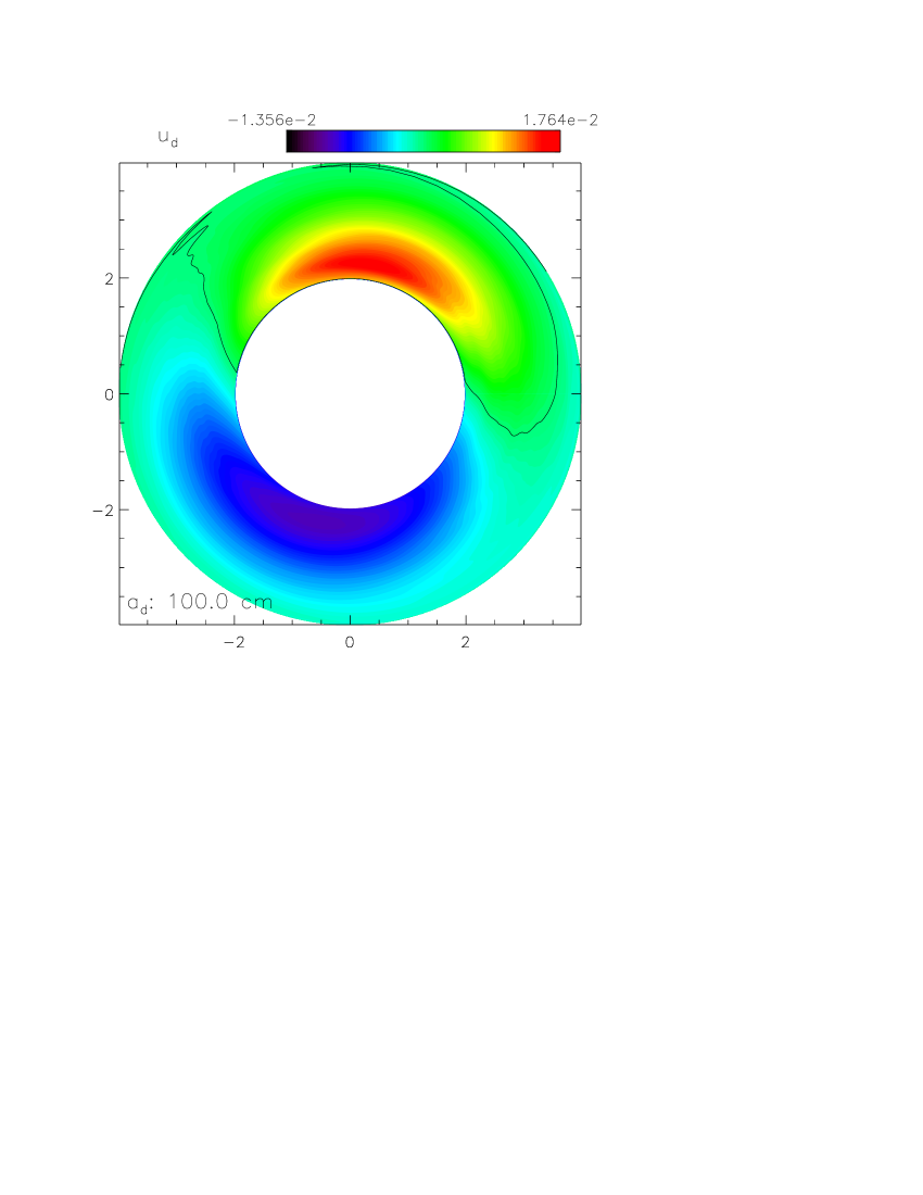
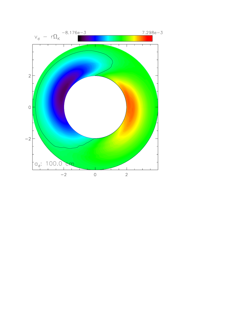
Figure 10: Dust velocity fields (left - radial; right - azimuthal) of the transition disk for the $e_{p}=0$ case for three particle sizes. The unit of the velocity is 2.98$\times 10^{5}$ cm/s.

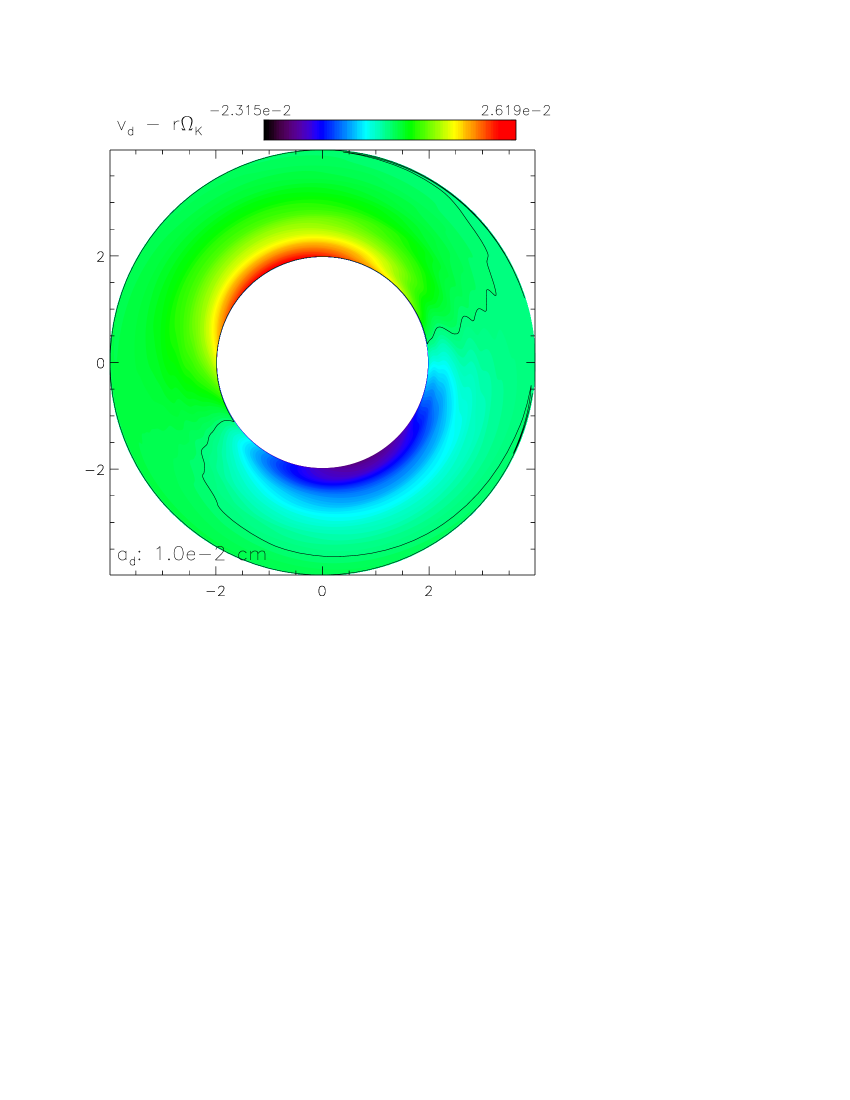
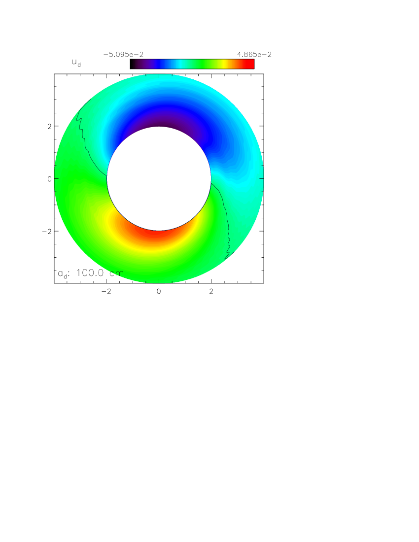
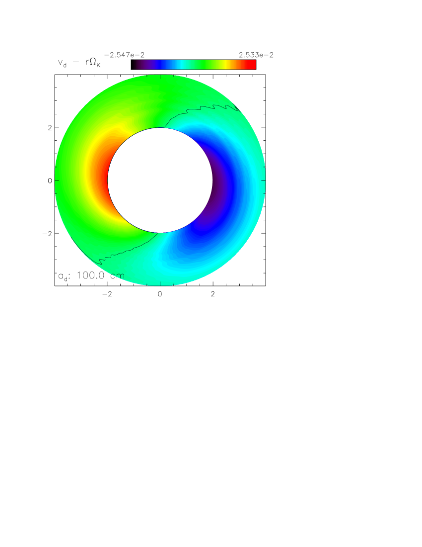
Figure 11: Same as Figure 10 but for the $e_{p}=0.1$ case.

The departures from the Keplerian circular velocity for particles of 3 different sizes (0.01, 1, and 100 cm) are shown in Figure 10 for $e_{p}=0$ and in Figure 11 for $e_{p}=0.1$. In comparison to the results from the gas velocity map in Figure 4, particles smaller than 1 cm are still tightly coupled to the gas but meter-sized particles become weakly coupled in the transition disk. As a result, the radial velocity of the gas and that of the well-coupled dust can reach about 167-171 m/s around the outer edge of the gap, while the radial velocity of meter-sized particles exhibit different magnitudes; namely, 40-53 m/s for $e_{p}=0$ and 145-152 m/s for $e_{p}=0.1$ at the outer edge of the gap. The larger velocity for the meter-sized particles in the $e_{p}=0.1$ case is due to excitation by the planet eccentricity. There exists a pronounced azimuthal phase difference in the velocities between the small and large particles.

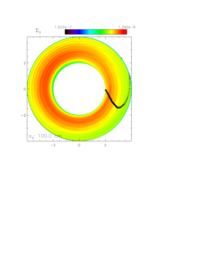
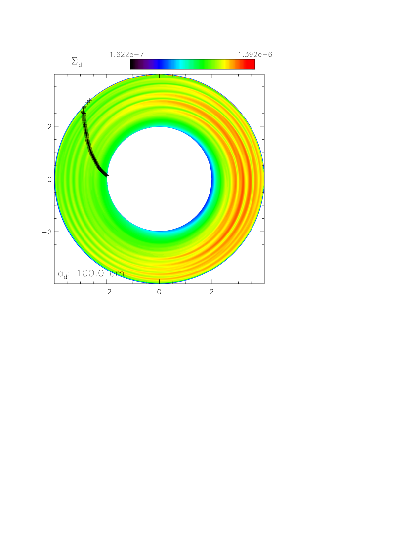
Figure 12: The dust surface density of various sizes in the transition disk for the $e_{p}=0$ (left panels) and $e_{p}=0.1$ (right panels) cases. The length unit is $a_{p}=100$ AU. The unit of the surface density is $8.89\times 10^{-4}$ g cm^-2.

Figure 12 shows the dust density distributions for the 3 different particle sizes in the transition disk. The dust density distribution is similar to that for the gas in the cases of the 0.01 cm-sized and 1 cm-sized dust particles. In both the $e_{p}=0$ and $e_{p}=0.1$ cases, the value of $\tau_{s,sec}$ in the exterior disk is about $10^{-(3-4)}$ for the 0.01 cm-sized particles, which is 100 times smaller than that for the 1 cm-sized particles and 4 orders of magnitude smaller than that for 100 cm-sized particles. Meter-sized particles are still in the Epstein regime but become weakly coupled to the gas due to the low gas density (i.e. $\tau_{s,sec}>1$). As a result, the spatial distribution appears to be distinctly different between small dust grains and meter-sized particles. The location of the pericenter at each annulus is denoted by the plus sign in Figure 12. As in the case for the standard disk discussed in §4.2, the apocenters of the transition disk are almost aligned. Further, the density excess (deficit) resides around the apocenter (pericenter) of the dust. In the $e_{p}=0$ case, the corresponding phase difference between the 1 cm- and 100 cm-sized particles is about 80^∘, as shown in the left panels of Figure 12, in agreement with $\arctan(\tau_{s,sec})\approx\arctan(10)$ as described in §3.1. Despite the phase difference, particles of different sizes regress with the gas disk at the same rate in the steady state. In the $e_{p}=0.1$ case, the pericenters of meter-sized particles are always close to the pericenter of the planet even though Figure 12 only shows a snap shot.

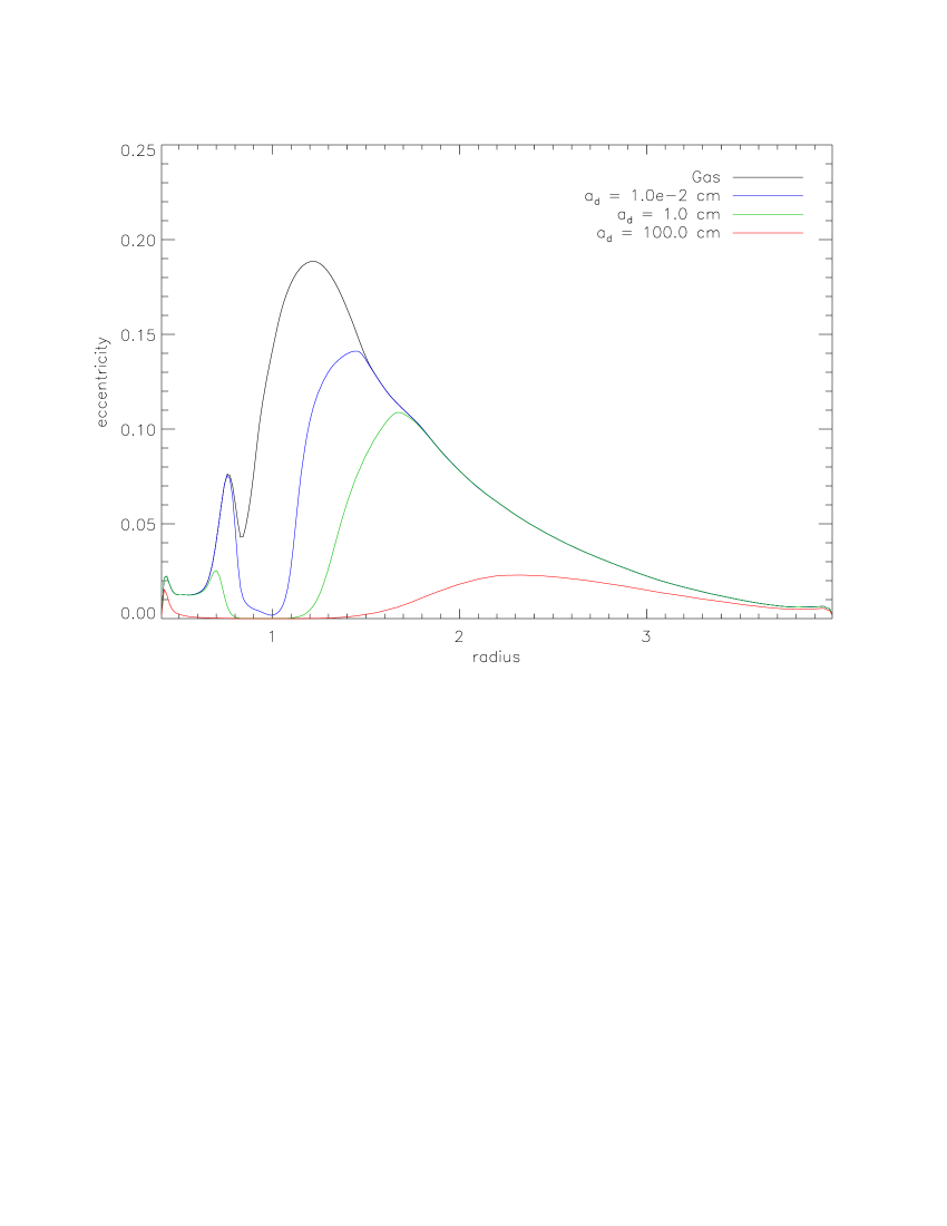
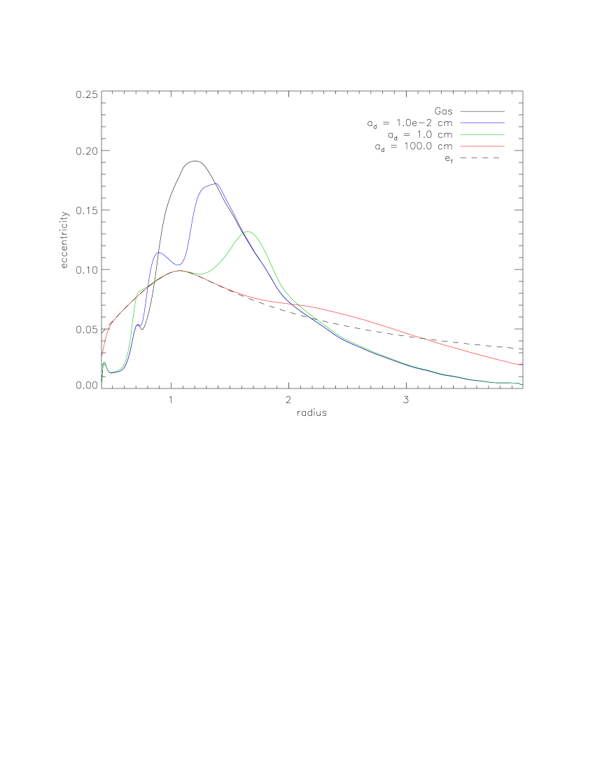
Figure 13: The azimuthal average of the dust and gas eccentricities for the transition disk. The left panel shows the case for $e_{p}=0$ and the right panel shows the cases for $e_{p}=0.1$. The forced eccentricity $e_{f}=|E_{f}|$ is also plotted for the $e_{p}=0.1$ case.

The azimuthal averages of dust and gas eccentricities are shown in Figure 13 for comparison. In the exterior disk for $e_{p}=0$ (left panel), the eccentricity of the weakly coupled particles marked in red (1 m) is smaller than that of well-coupled grains marked in blue (0.01 cm) and green (1 cm). In contrast, in the case of $e_{p}=0.1$ (right panel), the eccentricity of meter-sized particles become larger than that of the smaller dust in the region that our study focuses on (i.e. $r\geq 2$); the $e_{d}$ of the meter-sized particles is close to $e_{f}$, while the well-coupled dust (i.e. sizes smaller than 1 cm) still lies on the same eccentric orbits of the gas and thus regress with the gas disk. Because $\tau_{s,sec}\geq 1$ for meter-sized particles and Figure 13 shows that $e_{f}>e_{g}$, we have $\tau_{s,sec}e_{f}>e_{g}$. Thus, the orbits of the large particles librate instead of regressing with the gas. The libration rate equals the regression rate, as noted in §3.1. Additionally, at $r\gtrsim 2$, the value of $\tau_{s.sec}$ of meter-sized particles is the largest. It explains why the pericenters of meter-sized particles at such distances are close to the planetary pericenter.

As the dust particles become less coupled to the gas, the drag force wields less influence on the orbital motions of them. Therefore, the eccentric mode for dust excited by aerodynamic drag becomes less pronounced. It follows that in the absence of $e_{p}$, the weakly coupled particles are in near-Keplerian circular motions and thus their spatial distribution is close to axi-symmetric as manifested in the lower color contrast in the lower left panel of Figure 12. This leads to the lower density contrast for the meter-sized particles along the azimuthal direction of the disk. In the dimensionless unit, the density contrast for meter-sized particles is only about 5$\times 10^{-8}$ ($\sim 0.05\Sigma_{d,0}$), which is only a fraction of the density contrast $10^{-7}$ ($\sim 0.1\Sigma_{d,0}$) for smaller particles. In the case of $e_{p}=0.1$, the density contrast for the asymmetric distribution of meter-sized particles shown in the bottom right panel of Figure 12 is also about $5\times 10^{-8}$ ($\sim 0.05\Sigma_{d,0}$), despite the fact that their orbits are actually more eccentrically forced by the planetary eccentricity. This is because the eccentric gradient $de_{d}/dr$ is smaller, as shown in the right panel of Figure 13, leading to less compressive streamlines near the apocenter for meter-sized particles.

Finally we estimate the effect of the radial drift of the dust particles on their secular eccentric motion in the transition disk. We find that $t_{prec}/t_{drift}$ is on the order of $10^{-(0-2)}$ for the 0.01 cm-sized dust particles and $10^{-3}$ for the 100-cm particles. The ratio $t_{prec}/t_{drift}\sim 1$ for the 0.01 cm-sized dust only occurs near the location of $r=2$ where $\tau_{s}\sim 1$ and thus the radial drift is fast enough (Weidenschilling, 1977) to be comparable to the precession timescale. In contrast, the meter-sized dust drifts relatively slowly in the transition disk because their $\tau_{s}\gg 1$. Overall, in most of the region of the exterior disk, the ratio $t_{pres}/t_{drift}$ is small. This means that as in the case of the protoplanetary disk, particles smaller than 1 m drift slowly inwards to the adjacent eccentric orbit after a number of precessions in the transition disk.

5 SUMMARY AND DISCUSSIONS

We investigate the secular behavior of dust particles in a 2D eccentric protoplanetary disk harboring a massive planet. One fiducial model is considered with the following parameters: $M_{\star}=1\ M_{\odot}$, $M_{p}/M_{\star}\approx 5\times 10^{-3}$, $H/r=0.05$, $a_{p}=5$ AU, $\Sigma_{g}(t=0)=10^{-4}\times M_{*}/a_{p}^{2}=35.6$ g/cm², $\nu=10^{-5}\times a_{p}^{2}\Omega_{p}$, and the dust-to-gas ratio of the unperturbed disk is 0.01 everywhere.

The disk is assumed to be non-self-gravitating. We apply the fiducial model to the planet on a fixed circular and on a fixed eccentric orbit with $e_{p}=0.1$. We employ the FARGO code to extract the gas velocity and density from the 2-D hydrodynamical simulation, and then apply the eccentricity equation with the gas drag in the Epstein regime to study the dust dynamics. The simulations are performed for a sufficient length of time for the gas disk to attain quasi-steady states. To reveal the secular features of the disk, we average the gas properties over almost one planetary orbit in order to eliminate most of the short-period features associated with the spiral density waves driven by the orbital motion of the planet. Because the disk interior to the planet remains nearly circular in the model and the gas motions inside the gap deviate considerably from simple eccentric motions, we focus our study on the eccentric disk almost exterior to the gap, i.e. $2\leq r/a_{p}\leq 4$. The gap of the gas disk opened up by the planet on the eccentric orbit is slightly wider but a little shallower than that by the planet on the circular orbit. The gas disk regresses at the rate of about $(1/399)\Omega_{p}$ in the $e_{p}=0$ case and about $(1/152.8)\Omega_{p}$ in the $e_{p}=0.1$ case.

The most important parameter for determining the gas-dust coupling on the secular timescale in an eccentric disk is $\tau_{s,sec}$, the secular stopping time defined as the ratio of the stopping time to the precession timescale for a free particle. In our fiducial model for both the $e_{p}=0$ and $e_{p}=0.1$ cases, the spatial density distribution and velocity fields of dust particles of size smaller than 1 m are almost identical to those of the gas component due to the strong coupling through the gas drag (i.e. $\tau_{s,sec}\ll 1$). The perturbed velocities, defined as the velocity departures from the Keplerian circular orbit, are non-axisymmetric and exhibit the $m=1$ azimuthal profile with the phase difference of 90 degrees between the perturbed radial and azimuthal velocities as a consequence of the eccentric disk. The density also exhibits the $m=1$ distribution, with a $180^{\circ}$ phase difference relative to the perturbed azimuthal velocity. As a result, the density excess (deficit) lies around the apocenter (periceter) of the disk, with a magnitude of about 10% of the background dust density. Because the eccentricity decreases outwards from $e\approx 0.8$ at the outer edge of the gap, the $m=1$ structure is more prominent around the outer edge of the gap region. The perturbed velocity in this region is about 744.8 m/s.

We also apply the fiducial model to the transition disk defined in our work loosely by a protoplanetary disk with the overall low gas density equal to $8.89\times 10^{-2}$ g cm^-2. This is achieved by simply using the dimensionless results from the same simulation but with the planet placed at $a_{p}=100$ AU as the new length unit. In this low-density disk, meter-sized particles become weakly coupled to the gas (i.e. $\tau_{s,sec}>1$), while smaller particles still move closely with the gas on eccentric orbits (i.e. $\tau_{s,sec}\ll 1$). The velocity departures from the Keplerian circular motion for small dust particles can be as high as 167-171 m/s, and for meter-sized particles only reaches about 40-53 m/s in the $e_{p}=0$ case but can be excited to about 145-152 m/s in the $e_{p}=0.1$ case. Consequently in the $e_{p}=0$ case, meter-sized particles move in near-Keplerian circular orbits, which, in the steady state, regress at the same rate as the orbits of smaller dust particles but lag behind by about $80^{\circ}$. In the case of $e_{p}=0.1$, the orbits of the meter-sized particles are more eccentrically excited by the planetary eccentricity, with the pericenters roughly aligned with the pericenter of the planet’s orbit. The orbits of the meter-sized particles do not regress with the gas disk but librate around the location close to the pericenter of the planet. The $m=1$ density contrast resulting from the eccentric orbits is about 5% for meter-sized particles and about 10% for the smaller particles.

The presence of gas drag also causes radial drift of the dust. In our fiducial model for the protoplanetary and transition disks, the radial drift timescale is smaller than the precession timescale of dust particles smaller than 1 m in most regions of the eccentric disk. Therefore, the particles under consideration do not migrate inwards noticeably during the time for a few disk regressions. However, we anticipate that on the even longer timescale the dust eventually drifts to the outer edge of the gap, as in the case of a circular disk. Thus, the gap can act as a filter to stall the radial drift of large particles as proposed by Rice et al. (2006). We should also note that in our model for the transition disk, the slow radial drift of particles results from $\tau_{s}\gg 1$; namely, the gas becomes so tenuous that the particles are almost decoupled from the gas in one orbit. When taking into account any long-term disk evolution, it is conceivable that before the disk gradually loses mass and evolves to the transition disk, $\tau_{s}$ of dust particles of certain sizes is about 1. As a result, the eccentric disk almost loses dust particles of particular sizes before it becomes a transition disk. This happens to some extend in the simulation by Fouchet et al. (2010), where cm-sized particles are almost depleted in most part of the disk by radial drift as the disk evolves. By comparison, our model focuses on a particular stage with particles of all sizes present in the disk from $r=2$-4$a_{p}$, implying that we have assumed that dust particles are continuously replenished from the outer boundary. The evidence of gas replenishment to a protoplanetary disk at late stages has been suggested by the observation of the AB Aurigae disk (Tang et al., 2012).

Although the simulated gas disk in our model is not turbulent, the large kinematic viscosity $\nu$ is normally attributed to a turbulent flow. When the particles are well coupled to the gas such that $\tau_{s}\ll 1$, turbulent diffusion may be effective in smearing out the density inhomogeneity of dust. In a 2D disk, the rate for the turbulent diffusion is proportional to the divergence of $\Sigma_{g}(\nu/{\rm Sc})\nabla(\Sigma_{d}/\Sigma_{g})$ (e.g. Takeuchi & Lin, 2002), where Sc is the Schmidt number given approximately by $1+\tau_{s}^{2}$ (Youdin & Lithwick, 2007). In our model, where a constant and uniform dust-to-gas ratio in the basic state is assumed, $\nabla(\Sigma_{d}/\Sigma_{g})$ is almost zero for well coupled dust particles and thus the effect of turbulent diffusion is negligible. For meter-sized particles sufficiently decoupled from the gas in the transition disk, $\tau_{s}\gg 1$ and the timescale for the turbulent diffusion $\sim 10^{5}\tau_{s}^{2}(r/a_{p})^{2}/\Omega_{p}$, which is much larger than the regression/libration time $399/\Omega_{p}$ and $152.8/\Omega_{p}$. Therefore, turbulent diffusion is not important for the secular effects of our analysis.

In a circular disk, well-coupled dust particles can be temporarily trapped in the peaks of spiral density waves and more permanently in the Lindblad resonances (Paardekooper & Mellema, 2006). The eccentric disk harboring a planet of 5 Jupiter masses simulated by Fouchet et al. (2010) exhibited a great concentration of 1 cm-sized dust particles in the strong spiral wave just outside of the gap. In this work, we limit ourselves to the secular evolution of dust. Hence, whether these transient and resonant effects for dust trapping can also occur in an eccentric gaseous disk is not addressed.

Müller & Kley (2012) simulated eccentric circumstellar disks in binary star systems and investigated how different physical parameters affect disk evolutions. They showed that the gas eccentricity of a realistic radiative disk is smaller than that of a locally isothermal disk. As a result, the dust eccentricity is expected to be smaller than that in our results, and hence the asymmetric dust distribution in an eccentric disk would present more of a challenge for detection.

Other than the aforementioned effects that are ignored, several phenomena have also been left out in this work. In reality, dust particles can settle toward the mid-plane and influence the disk gas. The efficiency of the dust settling depends also on the stopping time, which evolves with the gas disk (Fouchet et al., 2010). The resulting thin, dense disk for dust with its relative motion to the gas leads to the streaming instability, which clumps the dust (Youdin & Goodman, 2005). We are unable to consider in our 2D model these effects involving vertical motions. In our model, dust of various sizes are assumed to be uniformly distributed after the planet-disk system settles into a quasi-steady state. We simply assume that the dust-to-gas ratio is so small that dust motions are passively influenced by the gas motions without any feedback to the gas dynamics. Another limitation of our model is that dust growth/fragmentation have not been taken into account. Collisions among large particles can produce smaller particles, which have the effect of smearing out the distinct phase differences of the asymmetric features between well and weakly coupled particles. Orbital crossing between strongly and weakly coupled dust particles surely enhances dust collisions and hence facilitates dust growth/fragmentation. Without considering these effects, the dust size distribution is thus not modelled in our study. Nevertheless, our work focussing only on secular dynamics of dust presents a framework for future studies to explore more complicated gas-dust dynamics in an eccentric disk.

Having described the limitations of our analysis, our results may render a basic picture for ALMA (Atacama Large Millimeter/submillimer Array) and EVLA (Karl G. Jansky Very Large Array) observations. The short-period features, such as the tightly wound density waves, probably present formidable challenges to be observationally resolved, but the secular features discussed in this study are more large-scale, comparable to the gap size, and thus more promising detection-wise. There exists a phase correlation for the $m=1$ structure between the gas velocity fields and dust density distribution in an eccentric disk with an embedded massive planet. The velocity departure from the Keplerian circular motion in our model can be larger than 150 m/s, which is probably high enough for ALMA detectability. In addition, the maximum dust emissions should be aligned with the apocenter of the eccentric gap in an eccentric disk. We show that particles with sizes of 1 m and 1 cm may be distributed differently in the azimuthal direction of an eccentric disk with a low gas density. Although large particles may be broken down into small dust particles, perhaps an attempt to measure the spectral energy distribution with EVLA in different azimuthal directions covering the wavelengths from 1 to tens of cm and to ascertain whether the dust sizes depend on the azimuthal angle of a transition disk with an eccentric gap is feasible.

The gap of the gaseous disk for $e_{p}=0.1$ is slightly shallower but wider than that for $e_{p}=0$ in our model for $q\approx 5\times 10^{-3}$. This outcome seems to be consistent with the parameter study by Hosseinbor et al. (2007) for smaller planetary masses $q\leq 10^{-3}$ on fixed orbits. Since we are concerned with dust dynamics exterior to the gap, the gap shape does not introduce significant differences in the results between the $e_{p}=0$ and $e_{p}=0.1$ cases. Nonetheless, it has been known from theories that in the presence of eccentricity, the planet-disk interaction does not depend only on the 3:1 eccentric Lindblad resonance but may rely on other resonances (Goldreich & Tremaine, 1980). Using the same code with the standard disk parameters, Hosseinbor et al. (2007) suggested that the planetary eccentricity enhances the torques on the gas via eccentric corotation resonances against the opposite torques from Lindblad resonances and thus results in more gas in the gap. The account does not explain why the gap opened up by an eccentric planet is wider, which occurs beyond the disk radius $r\approx 1.2$-1.3 as shown in their Figure 4 and in our Figure 2. Note that at $r\approx 1.587$, the 2:1 eccentric corotation resonance overlaps with the 4:2 eccentric Lindblad resonance as well as the 2:1 ordinary Lindblad resonance. Unfortunately, one is unable to deduce sufficient information from resonant torques (Goldreich & Tremaine, 1980) to determine the evolution of the system when both the disk and planet possess eccentricity (Ogilvie, 2007). Investigation following the method provided by Ogilvie (2007) is desirable for understanding the gap opening due to mean-motion resonances in an eccentric disk.

In addition, Hosseinbor et al. (2007) has cautioned that it is not self-consistent to assume a fixed planetary orbit in their study. Our work, based on the same assumption, is certainly plagued with the same problem. The eccentricity evolutions of the disk and the planet should be coupled (D’Angelo et al., 2006), especially when the disk-to-planet mass ratio is not negligibly small (Papaloizou et al., 2001; Rice et al., 2008). In the linear secular theory solving for eccentric modes of a coupled planet-disk system, the pericenter of the planet’s orbit should not stand still as is assumed in our model but rather precess as well. The precession rate is the eigenvalue of the coupled planet-disk problem (Goodchild & Ogilvie, 2006) and therefore should be the same as that of the disk. A self-consistent linear calculation as well as numerical works should be conducted in the context that we have presented here.

Needless to say, our fiducial model for protoplanetary and transition disks only presents suggestive results for azimuthal asymmetry of dust distributions in an eccentric disk. Parameter studies built on our fiducial model should be conducted to provide a more complete picture that encompasses a large variety of physical conditions for protoplanetary disks at different stages.

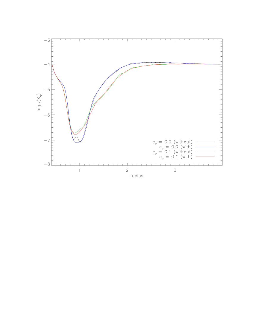
Figure 2: The azimuthal average of the gas densities shown in Figure 1. The gap in the $e_{p}=0.1$ case is wider but shallower than that in the $e_{p}=0$ case. The label “with (without)” denotes the azimuthal average with (without) time average.

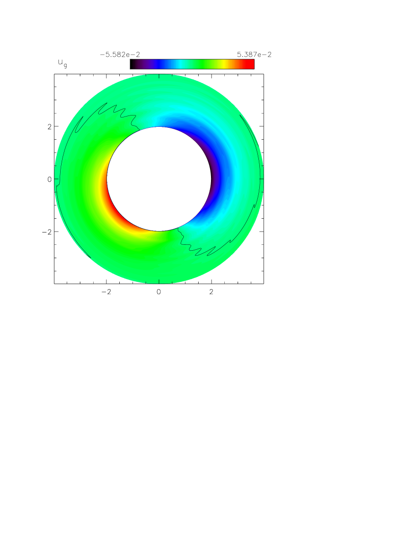
Figure 4: Gas velocity fields in the exterior disk associated with the density map shown in the time averaged bottom panels of Figure 1. The left panels show the radial gas velocity $u_{g}\approx u_{g,0}^{\prime}$ (top) and the azimuthal gas velocity departure from the Keplerian circular velocity $v_{g}^{\prime}=v_{g}-r\Omega_{K}\approx v_{g,0}^{\prime}$ (bottom) for the $e_{p}=0$ case. The right panels display $u_{g}$ and $v_{g}^{\prime}$ for the $e_{p}=0.1$ case. The zero values are denoted by the black curves.

References

- Andrews et al. (2011) Andrews, S. M. et al. 2011, ApJ, 732, 42
- Boss (2011) Boss, A. P. 2011, ApJ, 731, 74
- Crida et al. (2009) Crida, A., Masset, F., & Morbidelli, A. 2009, A&A, 502, 679
- D’Angelo et al. (2006) D’Angelo, G., Lubow, S. H., & Bate, M. R. 2006, ApJ, 652, 1698
- Fouchet et al. (2010) Fouchet, L, Gonzalez, J.-F., & Maddison, S. T. 2010, A&A, 518, 16
- Goldreich & Tremaine (1980) Goldreich & Tremaines 1980, ApJ, 241, 425