Symbolic Planning and Control Using Game Theory and Grammatical Inference

Abstract

This paper presents an approach that brings together game theory with grammatical inference and discrete abstractions in order to synthesize control strategies for hybrid dynamical systems performing tasks in partially unknown but rule-governed adversarial environments. The combined formulation guarantees that a system specification is met if (a) the true model of the environment is in the class of models inferable from a positive presentation, (b) a characteristic sample is observed, and (c) the task specification is satisfiable given the capabilities of the system (agent) and the environment.

I Introduction

I-A Overview

This paper demonstrates how a particular method of machine learning can be incorporated into hybrid system planning and control, to enable systems to accomplish complex tasks in unknown and adversarial environments. This is achieved by bringing together formal abstraction methods for hybrid systems, grammatical inference and (infinite) game theory.

Many, particularly commercially available, automation systems come with control user interfaces that involve continuous low-to-mid level controllers, which are either specialized for the particular application, or are designed with certain ease-of-use, safety, or performance specifications in mind. This paper proposes a control synthesis method that works with—rather than in lieu of—existing control loops. The focus here is on how to abstract the given low-level control loops [1] and the environment they operate in [2], and combine simple closed loop behaviors in an orchestrated temporal sequence. The goal is to do so in a way that guarantees the satisfaction of a task specification and is provably implementable at the level of these low-level control and actuation loops.

As a field of study, grammatical inference is primarily concerned with developing algorithms that are guaranteed to learn how to identify any member of a collection of formal objects (such as languages or graphs) from a presentation of examples and/or non-examples of that object, provided certain conditions are met [3]. The conditions are typical in learning research: the data presentation must be adequate, the objects in the class must be reachable by the generalizations the algorithms make, and there is often a trade-off between the two.

Here, grammatical inference is integrated into planning and control synthesis using game theory. Game theory is a natural framework for reactive planning of a system in a dynamic environment [4]. A task specification becomes a winning condition, and the controller takes the form of a strategy that indicates which actions the system (player 1) needs to take so that the specification is met regardless of what happens in its environment (player 2) [5, 6]. It turns out that interesting motion planning and control problems can be formulated at a discrete level as a variant of reachability games [7], in which a memoryless winning strategy can be computed for one of the players, given the initial setting of the game.

In the formulation we consider, the rules of the game are assumed to be initially unknown to the system; the latter is supposed to operate in a potentially adversarial environment with unknown dynamics. The application of grammatical inference algorithms to the observations collected by the system during the course of the game enables it to construct and incrementally update a model of this environment. Once the system has learned the true nature of the game, and if it is possible for it to win in this game, then it will indeed find a winning strategy, no matter how effectively the adversarial environment might try to prevent it from doing so. In other words, the proposed framework guarantees the satisfaction of the task specification in the face of uncertainty, provided certain conditions are met. If those conditions are not met, then the system is no worse off than when not using grammatical inference algorithms.

I-B Related work

So far, symbolic planning and control methods address problems where the environment is either static and presumably known, or satisfies given assumptions [8, 9, 10].

In cases where the environment is static and known, we see applications of formal methods like model checking [9, 11]. In other variants of this formulations, reactive control synthesis is used to tackle cases where system behavior needs to be re-planned based on information obtained from the environment in real time [8]. In [10] a control strategy is synthesized for maximizing the probability of completing the goal given actuation errors and noisy measurements from the environment. Methods for ensuring that the system exhibits correct behavior even when there is the mismatch between the actual environment and its assumed model are proposed in [12].

Linear Temporal Logic (LTL) plays an important role in existing approaches to symbolic planning and control. It is being used to capture safety, liveness and reachability specifications [13]. A formulation of LTL games on graphs is used in [14] to synthesize control strategies for non-deterministic transition systems. Assuming an uncertain system model, [12] combines temporal logic control synthesis with receding horizon control concepts. Centralized control designs for groups of robots tasked with satisfying a LTL-formula specification are found in [15], under the assumption that the environment in which the robots operate in adheres to certain conditions. These methods are extended [16] to enable the plan to be revised during execution.

Outside of the hybrid system’s area, adjusting unknown system parameters has traditionally been done by employing adaptive control or machine learning methods. Established adaptive control techniques operate in a purely continuous state regime, and most impose stringent conditions (e.g., linearity) on the system dynamics; for these reasons they are not covered in the context of this limited scope review—the interested reader is referred to [17, 18]. On the other hand, machine learning is arguably a broader field. A significant portion of existing work is based on reinforcement learning, which has been applied to a variety of problems such as multi-agent control [19], humanoid robots [20], varying-terrain wheeled robot navigation [21], and unmanned aerial vehicle control [22]. The use of grammatical inference as a sub-field of machine learning in the context of robotics and control is not entirely new; an example is the application of a grammatical inference machine (GIM) in robotic self-assembly [23].

In the aforementioned formulations there is no consideration for dynamic adversarial environments. A notable exception is the work of [24], which is developed in parallel to, and in part independently from, the one in this paper. The idea of combining learning with hybrid system control synthesis is a natural common theme since both methods originate from the same joint sponsored research project. Yet, the two approaches are distinct in how they highlight different aspects of the problem of synthesis in the presence of dynamic uncertainty. In [24], the learning module generates a model for a stochastic environment in the form of a Markov Decision Process and control synthesis is performed using model checking tools. In this paper, the environment is deterministic, but intelligently adversarial and with full knowledge of the system’s capabilities. In addition, the control synthesis here utilizes tools from the theory of games on infinite words.

I-C Approach and contributions

This paper introduces a symbolic control synthesis method based on the architecture of Fig. 1(a), where a GIM is incorporated into planning and control algorithms of a hybrid system (a robot, in Fig. 1(a)) to identify the dynamics of an evolving but rule-governed environment. The system—its boundaries outlined with a thick line—interacts with its environment through sensors and actuators. Both the system as well as its environment are dynamical systems (shown as ovals), assumed to admit discrete abstractions in the form of transition systems (dashed rectangles). The system is required to meet a certain specification. Given its specification ($\mathcal{A}_{s}$), an abstraction of itself ($A_{1}$), and its hypothesis of the dynamics of its environment ($A_{2}$), the system devises a plan and implements it utilizing a finite set of low-level concrete control loops involving sensory feedback. Using this sensory information, the system refines its discrete environment model based on a GIM, which is guaranteed to identify the environment dynamics asymptotically. Figure 1(b) gives a general description of the implementation of learning and symbolic planning at the high-level of the architecture in Fig. 1(a). The hypothesis on the environment dynamics is at the center of the system’s planning algorithm. Through interactions with the environment, the system observes the discrete evolution $\phi(i)$ of the environment dynamics, and uses the GIM to construct and update a hypothesized environment model $A_{2}^{(i)}$. Based on the environment model, the system constructs a hypothesis (model) $\mathcal{G}^{(i)}$ capturing how the “game” between itself and the environment is played, and uses this model to devise a winning strategy (control law) $\mathsf{WS}_{1}^{\ast}$. As the environment model converges asymptotically to the true dynamics $A_{2}$, the winning strategy becomes increasingly more effective. In the limit, the system is guaranteed to win the game.

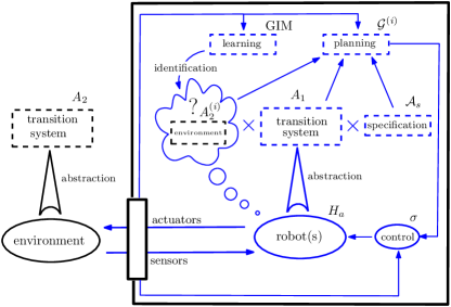
(a) An overview of the architecture

(b) Learning and planning with grammatical inference module at the higher level.

Figure 1: The architecture of hybrid agentic planning and control with a module for grammatical inference.

Definitions 7, 8 and Theorem 5 establish how a game can be constructed from the system abstractions of the (hybrid) system dynamics ($A_{1}$), the environmental dynamics ($A_{2}$), and the task specification ($\mathcal{A}_{s}$). Theorem 4 proves that the hybrid agent can determine whether a winning strategy exists, and if it does, what it is. Grammatical inference methods yield increasingly accurate models of environmental dynamics (assuming adequate data presentations and reachable targets), and permit the system to converge to an accurate model of its environment. Discrete backward reachability calculations can be executed in a straightforward manner and can allow the determination of winning strategies (symbolic control laws), whenever the latter exist.

The contribution of this paper is two-fold: (i) it integrates GIMs into hybrid systems for the purpose of identifying the discrete dynamics of the environment that evolve and possibly interact with the system, and (ii) it uses the theory of games on infinite words for symbolic control synthesis, and discrete abstractions which ensure implementation of the symbolic plans on the concrete hybrid system. In the paper, both elements are combined, but each element has merit even in isolation. A hybrid system equipped with GIM is still compatible with existing symbolic control synthesis methods (including model checking). On the other hand, the abstractions methods we utilize here—although requiring strong properties on the continuous components dynamics of the hybrid system—offer discrete abstract models which are weakly simulated by the concrete systems, irrespectively of whether the latter include a GIM or not.

I-D Organization

The rest of this paper is organized as follows. Section II introduces the technical background, the notation, and the models used. The type of hybrid systems considered and their discrete abstractions are presented there. In Section III, we show how the control problem can be formulated as a game and employ the concept of the attractor in games for control synthesis. Section IV describes first how a GIM can be used to identify asymptotically the dynamics of the system’s unknown and adversarial environment, and then how this knowledge can be utilized in planning and control synthesis. In Section V, we establish the properties of the relation between the hybrid system and its discrete abstraction, which ensure that the strategy devised based on the discrete model is implementable on the concrete system. Section VI illustrates the whole approach through an example robotic application. In Section VII we discuss possible extensions of the proposed methodology and compare our grammatical inference to other learning methods.

II Technical Preliminaries

II-A Languages and Grammatical Inference

Let $\Sigma$ denote a fixed, finite alphabet, and $\Sigma^{n}$, $\Sigma^{\leq n}$, $\Sigma^{*}$, $\Sigma^{\omega}$ be sequences over this alphabet of length $n$, of length less than or equal to $n$, of any finite length, and of infinite length, respectively. The empty string is denoted $\lambda$, and the length of string $w$ is denoted $|w|$. A language $L$ is a subset of $\Sigma^{*}$. A string $u$ is a prefix (suffix) of a string $w$ if and only if there exists a string $v$ such that $w=uv$ ($w=vu$). A prefix (suffix) of length $k$ of a string $w$ is denoted $\mathsf{Pr}^{=k}(w)$ (respectively, $\mathsf{Sf}^{=k}(w)$) and a set of prefixes (suffixes) of a string $w$ of length $\leq k$ is denoted as $\mathsf{Pr}^{\leq k}(w)$ (respectively, $\mathsf{Sf}^{\leq k}(w)$). For $w=\sigma_{1}\sigma_{2}\cdots\sigma_{n}\in\Sigma^{*}$, the shuffle ideal of $w$ is defined as $\mathsf{SI}(w):=\Sigma^{*}\sigma_{1}\Sigma^{*}\sigma_{2}\cdots\Sigma^{*}\sigma_{n}\Sigma^{*}$. A string $u$ is a factor of string $w$ iff $\exists x,y\in\Sigma^{*}$ such that $w=xuy$. If in addition $|u|=k$, then $u$ is a $k$-factor of $w$. If $E$ is a set, $2^{E}$ denotes the set of all subsets and $2_{\mathsf{fin}}^{E}$ the set of all finite subsets of $E$. A string extension function (SEF) is a total function, $\mathfrak{f}:\Sigma^{\ast}\rightarrow 2_{\mathsf{fin}}^{E}$. The k-factor function $\mathfrak{f}_{k}:\Sigma^{*}\rightarrow 2_{\mathsf{fin}}^{\Sigma^{\leq k}}$ maps a word to the set of $k$-factors within it. If $|w|\leq k$, $\mathfrak{f}_{k}(w):=\{w\}$, otherwise $\mathfrak{f}_{k}(w):=\{u\mid u\mbox{ is a }k\mbox{-factor of }w\}$. This function is extended to languages as $\mathfrak{f}_{k}(L):=\bigcup_{w\in L}\mathfrak{f}_{k}(w)$.

A semiautomaton (SA) is a tuple $A=\langle Q,\Sigma,T\rangle$ where $Q$ is the set of states, $\Sigma$ is the set of alphabet and the transition function is $T:Q\times\Sigma\rightarrow Q$. The elements of $\Sigma$ are referred to as actions and are thought to initiate transitions at a given state according to $T$. If $T(q_{1},\sigma)=q_{2}$ (also written as $q_{1}\stackrel{{\scriptstyle\sigma}}{{\rightarrow}}q_{2}$) with $\sigma\in\Sigma$, then we say that $A$ takes action $\sigma$ on $q_{1}$ and moves to $q_{2}$. The transition function is expanded recursively in the usual way. Note by definition, these SAs are deterministic in transition. For a (semi)automaton $A$, we define the set-valued function $\Gamma:Q\rightarrow 2^{\Sigma}$ as $\Gamma(q):=\{\sigma\in\Sigma\mid T(q,\sigma)\mbox{ is defined}\}$. A finite state automaton (FSA) is a tuple $\mathcal{A}=\langle A,I,F\rangle$ where $A=\langle Q,\Sigma,T\rangle$ is a semiautomaton and $I,F\subseteq Q$ are the initial and final states, respectively. The language of a FSA is $L(\mathcal{A}):=\{w\mid T(I,w)\cap F\neq\emptyset\}$. For a regular language $L$, deterministic FSAs recognizing $L$ with the fewest states are called canonical.

For concreteness, let grammars of languages be constructed as the set of possible Turing machines $\mathfrak{G}$. (Other kinds of grammars are used later, but they are translatable into Turing machines.) The language of a particular grammar $\mathfrak{G}$ is $L(\mathfrak{G})$. A positive presentation $\phi$ of a language $L$ is a total function $\phi:\mathbb{N}\rightarrow L\cup\{\#\}$ ($\#$ is a ‘pause’) such that for every $w\in L$, there exists $n\in\mathbb{N}$ such that $\phi(n)=w$. With a small abuse of notation, a presentation $\phi$ can also be understood as an infinite sequence $\phi(1)\phi(2)\cdots$ containing every element of $L$.

Let $\phi[i]$ denote the initial finite sequence $\phi(1)\phi(2)\ldots\phi(i)$. Let $\mathfrak{Seq}$ denote the set of all finitely long initial portions of all possible presentations of all possible languages (i.e., all $\phi[i]$ for all $i\in\mathbb{N}$ and for all $L$). The content of $\phi[i]$, written $\textsf{content}(\phi[i])$, is the set of the elements of the sequence, less the pauses. A learner (learning algorithm, or GIM) is a program that takes the first $i$ elements of a presentation and returns a grammar as output: $\mathfrak{Gim}:\mathfrak{Seq}\to\mathfrak{G}$. The grammar returned by $\mathfrak{Gim}$ is the learner’s hypothesis of the language. A learner $\mathfrak{Gim}$ identifies in the limit from positive presentations of a collection of languages $\mathcal{L}$ if and only if for all $L\in\mathcal{L}$, for all presentations $\phi$ of $L$, there exists a $n\in\mathbb{N}$ such that for all $m\geq n$, $\mathfrak{Gim}(\phi_{m})=\mathfrak{G}$ and $L(\mathfrak{G})=L$ [25]. A characteristic sample $S$ for a language $L$ and a learner $\mathfrak{Gim}$ is a finite set of strings belonging to $L$ such that for any $\phi[i]$ such that $\mathsf{content}(\phi[i])=S$, it is the case that for all $j\geq i$, $\mathfrak{Gim}(\phi[j])=\mathfrak{G}$ and $L(\mathfrak{G})=L$.

Definition 1 (String extension grammar and languages [26])

Let $\mathfrak{f}$ be a SEF, and $E$ be a set. A string extension grammar $\mathfrak{G}$ is a finite subset of $E$. The string extension language of grammar $\mathfrak{G}$ is $L_{\mathfrak{f}}(\mathfrak{G})=\{w\in\Sigma^{\ast}:\mathfrak{f}(w)\subseteq\mathfrak{G}\}.$ The class of string extension languages is $\mathcal{L}_{\mathfrak{f}}:=\{L_{\mathfrak{f}}(\mathfrak{G}):\mathfrak{G}\in 2_{\mathsf{fin}}^{E}\}.$

Definition 2 (String Extension Learner[26])

Let $\mathfrak{f}$ be a SEF. For all positive presentations $\phi$, define $\mathfrak{Gim}_{\mathfrak{f}}$ as: $\mathfrak{Gim}_{\mathfrak{f}}(\phi[i])=\emptyset$ if $i=0$, and

$$\mathfrak{Gim}_{\mathfrak{f}}(\phi[i]):=\begin{cases}\mathfrak{Gim}_{\mathfrak{f}}(\phi[i-1])&\text{ if }\phi(i)=\#\\ \mathfrak{Gim}_{\mathfrak{f}}(\phi[i-1])\cup\mathfrak{f}(\phi[i])&\text{ otherwise}\enspace.\end{cases}$$ (1)

According to [25], the class of regular languages is not identifiable in the limit from positive presentation, but string extension languages—which are subclasses of regular languages—are.

Theorem 1 (​​[26])

Learner $\mathfrak{Gim}_{\mathfrak{f}}$ identifies $\mathcal{L}_{\mathfrak{f}}$ in the limit.

Many attractive properties of string extension learners are established in [27]. A language $L$ is Strictly $k$-Local ($\text{ \acl{sl} (\acs{sl})}_{k}$) [28, 29] iff there exists a finite set $S\subseteq\mathfrak{f}_{k}(\rtimes\Sigma^{*}\ltimes)$, such that $L=\{w\in\Sigma^{*}:\mathfrak{f}_{k}(\rtimes w\ltimes)\subseteq S\}$, where $\rtimes,\ltimes$ are the symbols indicating the beginning and end of a string, respectively. Obviously, Strictly $k$-Local languages are string extension languages. The following theorem follows immediately.

Theorem 2 (​​[30])

For every $k$, Strictly $k$-Local languages are identifiable in the limit from positive presentations.

Theorem 3 (SL-Hierarchy ​​[31])

$\text{ \acs{sl}}_{1}\subset\text{\acs{sl}}_{2}\subset\ldots\subset\text{\acs{sl}}_{i}\subset\text{\acs{sl}}_{i+1}\subset\ldots\text{\acs{sl}}$.

The implication of Theorem 3 is that any Strictly $k$-Local language can be described using a SL_j grammar, where $j\geq k$. Section IV illustrates this argument with the help of an example.

II-B Hybrid Systems and Abstractions

A hybrid system $H$ is defined as a tuple of objects (for a precise definition, see [32]) that includes the domains of continuous and discrete variables, the subsets of initial states in those domains, the description of the family of continuous dynamics parametrized by the discrete states, and rules for resetting continuous and discrete states and switching between the members of the family of continuous dynamics.

In this paper, we restrict our attention to a specific class of hybrid systems where the continuous dynamics have specific (set) attractors [1]. The shape and location of these attractors are assumed dependent on a finite set of continuous parameters that are selected as part of closing the outer control loop. Judicious selection of the parameters activates a specific sequence of continuous and discrete transitions, which in turn steers the hybrid system $H$ from a given initial state to a final desired state. This class admits purely discrete (predicate-based) abstractions. We call these particular types of hybrid automata hybrid agents, to distinguish them from general cases.

Definition 3 (Hybrid Agent)

The hybrid agent is a tuple:

$H_{a}=\langle{\mathcal{Z},\Sigma_{a},\iota,\mathcal{P},\pi_{i},\mathcal{AP},f_{\sigma},\text{{Pre}},\text{{Post}},s,T_{a}}\rangle$.

• $\mathcal{Z}={\cal X}\times{\bm{L}}$ is a set of composite (continuous and Boolean) states, where ${\cal X}\subset\mathbb{R}^{n}$ is a compact set, and ${\bm{L}}\subseteq\left\{{\bm{0,1}}\right\}^{r}$ where $r$ is the number of Boolean states.

• $\Sigma_{a}$ is a set of finite discrete states (control modes).

• $\iota:\Sigma_{a}\to\{1,\ldots,k\}$ is a function, indexing the set of symbols in $\Sigma_{a}$.

• $\mathcal{P}\subseteq\mathbb{R}^{m}$ is a (column) vector of continuous parameters.

• $\pi_{i}:\mathbb{R}^{m}\to\mathbb{R}^{m_{i}}$, for $i=1,\ldots,k$ is a finite set of canonical projections, such that $p=(\pi_{1}(p)^{\mathsf{T}},\ldots,\pi_{k}(p)^{\mathsf{T}})^{\mathsf{T}}$.

• $\cal{AP}$ is a set of (logical) atomic propositions over $\mathcal{Z}\times\mathcal{P}$, denoted $\{\alpha_{h}(z,p)\}_{i=1}^{|\mathcal{AP}|}$. A set of well-formed formulae $\mathsf{WFF}$ [33] is defined inductively as follows: (a) if $\alpha\in\mathcal{AP}$, then $\alpha\in\mathsf{WFF}$; (b) if $\alpha_{1}$ and $\alpha_{2}$ are in $\mathsf{WFF}$, then so are $\neg\alpha_{1}$ and $\alpha_{1}\land\alpha_{2}$.

• $f_{\sigma}$: $\mathcal{Z}\times{\cal{P}}\to T{\cal{X}}$ is a finite set of families of vector fields parametrized by $p\in\mathcal{P}$, $\ell\in\bm{L}$ and $\sigma\in\Sigma$, with respect to which $\mathcal{X}$ is positively invariant. These vector fields have limit sets parametrized by $p$ and $\sigma$, denoted $L^{+}(p,\sigma)$.

• Pre: $\Sigma_{a}\to\mathsf{WFF}$ maps a discrete state to a formula that needs to be satisfied whenever $H_{a}$ switches to discrete state $\sigma$ from any other state. When composite state $z$ and parameter vector $p$ satisfy this formula we write $(z,p)\models\text{{Pre}}(\sigma)$.

• Post: $\Sigma_{a}\to\mathsf{WFF}$ maps a discrete location to a formula that is satisfied when the trajectories of $f_{\sigma}$ reach an $\epsilon$-neighborhood of their limit set. When composite state $z$ and parameter vector $p$ satisfy this formula we write $(z,p)\models\text{{Post}}(\sigma)$.

• $s$: ${\cal Z}\times{\cal P}\rightarrow 2^{\cal P}$ is the reset map for the parameters. It assigns to each pair of composite state and parameter a subset of $\cal P$ which contains all values to which the current value of $p\in\cal P$ can be reassigned to.

• $T_{a}$: ${\cal Z}\times{\cal P}\times{\Sigma_{a}}\rightarrow{\cal Z}\times{\cal P}\times{\Sigma_{a}}$ is the discrete state transition map, according to which $\left(z,p,\sigma\right)\to\left(z,p^{\prime},\sigma^{\prime}\right)$ iff $(z,p)\models\text{{Post}}(\sigma)$ and $(z,p^{\prime})\models\text{{Pre}}(\sigma^{\prime})$ with $p^{\prime}\in s(z,p)$.

The configuration of $H_{a}$ is denoted $h:=[z,p,\sigma]$, and for each discrete state, we define the following subsets of $\mathcal{Z}\times\mathcal{P}$: $\overleftarrow{\sigma}:=\{(z,p):(z,p)\models\text{{Pre}}(\sigma)\}$ and $\overrightarrow{\sigma}:=\{(z,p):(z,p)\models\text{{Post}}(\sigma)\}$. A transition from $\sigma_{i}$ to $\sigma_{i+1}$ (if any) is forced and occurs at the time instance when the trajectory of $f_{\sigma_{i}}\left(x,\ell,p\right)$ hits a nonempty intersection of a $\varepsilon$-neighborhood of its limit set and the region of attraction of $\sigma_{i+1}$ parametrized by $p^{\prime}$ ($p^{\prime}$ not necessarily equals $p$.) After a transition $\left(z,p,\sigma\right)\to\left(z,p^{\prime},\sigma^{\prime}\right)$ occurs, the composite state $z$ evolves into composite state $z^{\prime}$ for which $(z^{\prime},p^{\prime})\models\text{{Post}}(\sigma^{\prime})$. The (non-instantaneous) evolution is denoted $z\stackrel{{\scriptstyle\sigma^{\prime}[p^{\prime}]}}{{\hookrightarrow}}z^{\prime}$.

We will use a form of predicate abstraction to obtain a coarse, discrete representation of $H_{a}$. Our abstraction map is denoted $V_{M}:\mathcal{Z}\times\mathcal{P}\to\{\boldsymbol{0},\boldsymbol{1}\}^{|\mathcal{AP}|}$ and referred to as the valuation map:

Definition 4 (Valuation map)

The valuation map $V_{M}$: ${\mathcal{Z}\times\cal P}\to{\cal V}\subseteq\left\{\bm{1,0}\right\}^{|\cal{AP}|}$ is a function that maps pairs of composite states and parameters, to a binary vector $v\in\mathcal{V}$ of dimension $|\mathcal{AP}|$. The element at position $i$ in $v$, denoted $v[i]$, is $\bm{1}$ or $\bm{0}$ if $\alpha_{i}\in\mathcal{AP}$ is true or false, respectively, for a particular pair $(z,p)$. We write $\alpha_{i}(z,p)=v[i]$, for $v\in\cal V$.

The purely discrete model that we use as an abstraction of $H_{a}$, referred to as the induced transition system is defined in terms of the valuation map as follows.

Definition 5 (Induced transition system)

A hybrid agent $H_{a}$ induces a semiautomaton $A(H_{a})=\langle Q,\Sigma,T\rangle$ in which (i) $Q=V_{M}(\mathcal{Z}\times\mathcal{P})$is a finite set of states; (ii) $\Sigma=\Sigma_{a}\cup\{\tau_{1},\ldots,\tau_{m}\}$, $m\leq|Q\times Q|$ is a finite set of labels; (iii) $T\subseteq Q\times\Sigma\times Q$is a transition relation with the following semantics: $q\stackrel{{\scriptstyle\sigma}}{{\rightarrow}}q^{\prime}\in T$ iff either (1) $\sigma\in\Sigma_{a}$and $\left(\exists p\right)\left(\forall z\in\{z\mid V_{M}(z,p)=q\}\right)$ $\left(\forall z^{\prime}\in\{z^{\prime}\mid(z^{\prime},p)\models\text{{Post}}(\sigma)\}\right)$ $\left[(z,p)\models\text{{Pre}}(\sigma),V_{M}(z^{\prime},p)=q^{\prime}\right]$, or (2) $\sigma\in\Sigma\setminus\Sigma_{a}$and $\left(\exists p\right)$ $\left(\forall z\in\{z\mid V_{M}(z,p)=q\}\right)(\exists p^{\prime}\in s(z,p),\sigma^{\prime}\in\Sigma_{a})\left[V_{M}(z,p^{\prime})=q^{\prime},\,(z,p^{\prime})\models\text{{Pre}}(\sigma^{\prime})\right]$.

It will be shown in Section V that $H_{a}$ and $A(H_{a})$ are linked through an equivalence relation – observable (weakly) simulation relation. Broadly speaking, the sequences (strings in ${\Sigma_{a}}^{\ast}$) of discrete states which $H_{a}$ visits starting from $[z,p,\sigma]$ can be matched by a word $w$ such that $T\big{(}V_{M}(z,p),w\big{)}$ is defined in $A(H_{a})$, and vice versa, modulo symbols in $\Sigma\setminus\Sigma_{a}$ that are thought of as silent. When a SA moves from state $q$ to state $q^{\prime}$ through a series of consecutive transitions among which only one is labeled with $\sigma\in\Sigma_{a}$ and all others in $\Sigma\setminus\Sigma_{a}$, then we say that the SA takes a composite transition from $q$ to $q^{\prime}$, labeled with $\sigma$, and denoted $q\stackrel{{\scriptstyle\sigma}}{{\leadsto}}q^{\prime}$.

Definition 6 (Weak (observable) simulation [35])

Consider two (labeled) semiautomata over the same input alphabet $\Sigma$, $A_{1}=\langle Q_{1},\Sigma,\leadsto_{1}\rangle$ and $A_{2}=\langle Q_{2},\Sigma,\leadsto_{2}\rangle$, and let $\Sigma_{\epsilon}\subset\Sigma$ be a set of labels associated with silent transitions. An ordered binary relation $\mathfrak{R}$ on $Q_{1}\times Q_{2}$ is a weak (observable) simulation if: (i) $\mathfrak{R}$is total, i.e., for any $q_{1}\in Q_{1}$ there exists $q_{2}\in Q_{2}$ such that $(q_{1},q_{2})\in\mathfrak{R}$, and (ii) for every ordered pair $(q_{1},q_{2})\in{\mathfrak{R}}$ for which there exists $q_{1}^{\prime}$ such that $q_{1}\stackrel{{\scriptstyle\sigma}}{{\leadsto_{1}}}q_{1}^{\prime}$, then $\exists\;(q_{1}^{\prime},q_{2}^{\prime})\in\mathfrak{R}:q_{2}\stackrel{{\scriptstyle\sigma}}{{\leadsto_{2}}}q_{2}^{\prime}$. Then $A_{2}$ weakly simulates $A_{1}$ and we write $A_{2}\gtrsim A_{1}$.

Task specifications for hybrid systems (and transition systems, by extension) may be translated to a Kripke structure [36] (see [9] for examples), which is basically a SA with marked initial states, equipped with a labeling function that maps a state into a set of logic propositions that are true at that state. In this paper we also specify final states, and allow the labeling function to follow naturally from the semantics of the valuation map. We thus obtain a FSA $\mathcal{A}_{s}=\langle Q_{s},\Sigma_{s},T_{s},I_{s},F_{s}\rangle$, where $I_{s}$ and $F_{s}$ denote the subsets of initial and final states, respectively. Given the dynamic environment, a system ($H_{a}$ or $A(H_{a})$) satisfies the specification $\mathcal{A}_{s}$ if the interacting behavior of the system and the environment forms a word that is accepted in $\mathcal{A}_{s}$.

II-C Games on Semiautomata

Here, we follow for the most part the notation and terminology of [37, Chapter 4]. Let $A_{1}=\langle Q_{1},\Sigma_{1},T_{1}\rangle$ represents the dynamics of player 1, and $A_{2}=\langle Q_{2},\Sigma_{2},T_{2}\rangle$ those of player 2. We define the set $I_{i}\subseteq Q_{i}$ as the set of legitimate initial states of $A_{i}$, for $i=1,\,2$ respectively, but we do not specify final states in these two SA. The language admissible in $A_{i}$ is $\mathcal{L}(A_{i})=\bigcup_{q_{0}\in I_{i}}\bigcup_{q\in Q_{i}}\{w\mid T_{i}(q_{0},w)=q\}$, which essentially includes all possible sequences of actions that can be taken in $A_{i}$. Let $\Lambda=\Sigma_{1}\cup\Sigma_{2}$. Define an (infinite) game [37] $\mathcal{G}(\Phi)$ on $\Lambda$ as a set $\Phi\subset\Lambda^{\omega}$ of infinite strings consisted of symbols from the two alphabets $\Sigma_{1}$ and $\Sigma_{2}$ taken in turns. A play is an infinite string $w=\sigma_{1}\sigma_{2}\cdots\in\Lambda^{\omega}$. Players take turns with player 1 playing $\sigma_{1}$ first by default. In this paper we assume that players can give up their turn and “play” a generic (silent) symbol $\epsilon$, i.e. $\epsilon\in\Sigma_{i}$ and $T_{i}(q,\epsilon)=q$, $\forall\,q\in Q_{i}$. A pair of symbols $\sigma_{2i-1}\sigma_{2i}$ for $i=1,\ldots$ denotes a round, with any one of the two symbols being possibly equal to $\epsilon$. We say that player 1 wins the game if $w\in\Phi$; if not, then player 2 wins. A strategy for player $i$ in game $\mathcal{G}(\Phi)$ is a function $\mathsf{S}_{i}:\Lambda^{\ast}\to\Sigma_{i}$. Player 1 (2) follows strategy $\mathsf{S}_{1}$ (respectively, $\mathsf{S}_{2}$) in a play $w=\sigma_{1}\sigma_{2}\cdots$ if for all $n\geq 1$, $\sigma_{2n-1}=\mathsf{S}_{1}(\sigma_{1}\sigma_{2}\cdots\sigma_{2n-2})$ (respectively, $\sigma_{2n}=\mathsf{S}_{2}(\sigma_{1}\sigma_{2}\cdots\sigma_{2n-1})$). A strategy for player 1 is a winning strategy $\mathsf{WS}_{1}$ if all strings $w=\sigma_{1}\sigma_{2}\cdots$ that satisfy $\sigma_{2n-1}=\mathsf{WS}_{1}(\sigma_{1}\sigma_{2}\cdots\sigma_{2n-2}),\,\forall n\geq 1$, belong in $\Phi$. Winning strategies for player 2 are defined similarly. If one of the players has a winning strategy, then the game is determined.

III Game Theoretic Approach to Planning

III-A Constructing the game

Consider a hybrid agent having to satisfy a task specification, encoded in a FSA $\mathcal{A}_{s}$. Assume that this agent is operating in an unknown environment. In the worst case, this environment is controlled by an intelligent adversary who has full knowledge of the agent’s capabilities. The adversary is trying to prevent the agent from achieving its objective. The behavior of the environment is still rule-based, i.e. subject to some given dynamics, although this dynamics is initially unknown to the agent.

Assume that the agent has been abstracted to a SA $A_{1}$ (player 1) and the dynamics of the environment is similarly expressed in another SA $A_{2}$ (player 2). Without loss of generality, we assume the alphabets of $A_{1}$ and $A_{2}$ are disjoint, i.e. $\Sigma_{1}\neq\Sigma_{2}$. In this game, the agent is not allowed to give up turns ($\epsilon\notin\Sigma_{1}$) but the adversary that controls the environment can do so ($\epsilon\in\Sigma_{2}$). For two-player turn-based games, the actions of one player may influence the options of the other by forbidding the latter to initiate certain transitions. To capture this interaction mechanism we define the interaction functions $U_{i}:Q_{i}\times Q_{j}\rightarrow 2^{\Sigma_{j}},(i,j)\in\{(1,2),(2,1)\}$. An interaction function $U_{i}$ maps a given pair of states $(q_{i},q_{j})$ of players $i$ and $j$, to the set of actions player $j$ is not allowed to initiate at state $q_{j}$.

We now define a SA that abstractly captures the dynamics of interaction between the two players, by means of a new operation on SA which we call the turn-based product. An intersection of the turn-based product with the task specification yields the representation of the game and further allows us to compute the strategy for the agent.

Definition 7 (Turn-based product)

Given two SAs for players $A_{1}=\langle Q_{1},\Sigma_{1},T_{1}\rangle$ and $A_{2}=\langle Q_{2},\Sigma_{2},T_{2}\rangle$ with the sets of legitimate initial states $I_{1},\,I_{2}$ and interacting functions $U_{1},\,U_{2}$, their turn-based product $P=\langle Q_{p},\Sigma_{1}\cup\Sigma_{2},T_{p}\rangle$ is a SA denoted $A_{1}\circ A_{2}$, and is defined as follows:

• $Q_{p}=Q_{1}\times Q_{2}\times\left\{\bm{0},\bm{1}\right\}$, where the last component is a Boolean variable $c\in\left\{\bm{0},\bm{1}\right\}$ denoting who’s turn it is to play: $c=\bm{1}$ for player 1, $c=\bm{0}$ for player 2.

• $T_{p}\big{(}(q_{1},q_{2},c),\sigma\big{)}=(q_{1}^{\prime},q_{2},\bm{0})$ if $c=\bm{1},\;q_{1}^{\prime}=T_{1}(q_{1},\sigma)$, with $\sigma\notin U_{2}(q_{2},q_{1})$ and $T_{p}\big{(}(q_{1},q_{2},c),\sigma\big{)}$ $=(q_{1},q_{2}^{\prime},\bm{1})$ if $c=\bm{0},\;q_{2}^{\prime}=T_{2}(q_{2},\sigma)$, with $\sigma\notin U_{1}(q_{1},q_{2})$.

Assuming player 1 is the first one to make a move, the set of legitimate initial states in $P$ is $I_{1}\times I_{2}\times\{\bm{1}\}$ and the language admissible in $P$ is $\mathcal{L}(P)=\bigcup_{q_{0}\in I_{1}\times I_{2}\times\{\bm{1}\}}\;\bigcup_{q\in Q_{p}}\left\{w\mid T_{p}(q_{0},w)=q\right\},$ the set of all possible plays between two players. Note that if one includes the silent action $\epsilon$ in $\Sigma_{i}$ for $i=1,2$, the players may not necessarily play in turns—as in the specific case of agent-environment interaction considered here. The product operation is still applicable as defined.

The turn-based product $P$ gives snapshots of different stages in a game. It does not capture any of the game history that resulted in this stage. Often, task specifications encoded in $\mathcal{A}_{s}$ involve a history of actions, and thus the winning conditions for player 1 cannot be encoded in $P$ by simply marking some states as final. We overcome the lack of memory in $P$ by taking its product with $\mathcal{A}_{s}$. Taking the product is suggested by the fact that player 1 can win the game (i.e. agent can satisfy the specification) only if $L(\mathcal{A}_{s})\cap\mathcal{L}(P)\neq\emptyset$. The technical complication is that the two terms in this product are heterogeneous: one is a SA and the other is a FSA. We resolve this by transforming the SA into a FSA and applying the standard product operation; and the result is what we call the game automaton.

Definition 8 (Game automaton)

The game automaton is a FSA defined as $\mathcal{G}=\mathcal{P}\times\mathcal{A}_{s}=\langle Q,\Sigma,T,Q_{0},F\rangle$, where $\mathcal{A}_{s}=\langle Q_{s},\Sigma,T_{s},I_{s},F_{s}\rangle$ is a FSA encoding the winning conditions for player 1, and $\mathcal{P}$ is a FSA obtained from the turn-based product $P=A_{1}\circ A_{2}$ by defining the set of initial states of $\mathcal{P}$ as the legitimate initial states $I_{1}\times I_{2}\times\{\bm{1}\}$, and marking all other states as final. The set of initial states for $\mathcal{G}$ is defined as $Q_{0}=\{(q_{1},q_{2},\bm{1},q_{0s})\mid q_{1}\in I_{1},q_{2}\in I_{2},\;q_{0s}\in I_{s}\}$. The set of final states for $\mathcal{G}$ is given by $F=\{(q_{1},q_{2},\bm{0},q_{s})\mid q_{s}\in F_{s}\}$.

It follows (from the fact that the language of $\mathcal{G}$ is regular) that the game defined by $\mathcal{G}$ is a reachability game [38], and therefore it is determined. Note that the final states of $\mathcal{G}$ are exactly those in which player 1 wins the game. On FSA $\mathcal{G}$, we define the attractor of $F$, denoted $\mathsf{Attr}(F)$, which is the largest set of states $W\supseteq F$ in $\mathcal{G}$ from where player 1 can force the play into $F$. It is defined recursively as follows. Let $W_{0}=F$ and set

$$W_{i+1}:=W_{i}\cup\{q\in Q\mid q=(q_{1},q_{2},\bm{1},q_{s}),\text{ and }\exists\sigma\in\Gamma(q):T(q,\sigma)\in W_{i}\}\\ \cup\{q\in Q\mid q=(q_{1},q_{2},\bm{0},q_{s}),\text{ and }\forall\sigma\in\Gamma(q):T(q,\sigma)\in W_{i}\}\enspace.$$ (2)

The function $\rho:Q\to\mathbb{N};\;\rho(q)\mapsto\min\{i\geq 0\mid q\in W_{i}\}$ is called the rank function of the game.

Since $\mathcal{G}$ is finite, there exists the smallest $m\in\mathbb{N}$ such that $W_{m+1}=W_{m}$. Then $\mathsf{Attr}(F)=W_{m}$. Moreover, because $\mathcal{G}$ is determined, the complement of $\mathsf{Attr}(F)$ in $Q$ forms a trap for player 1; it contains all the states at which player 2 can prevent player 1 from winning the game. $\mathsf{Attr}(F)$ can be computed in time $\mathcal{O}(n_{1}+n_{2})$ where $n_{1}=|Q|$ and $n_{2}$ is the number of transitions in $\mathcal{G}$.

III-B Computing a winning strategy

The following statement is straightforward.

Theorem 4

Player 1 has a winning strategy iff $\mathsf{Attr}(F)\cap Q_{0}\neq\emptyset$.

Proof:

If $\mathsf{Attr}(F)\cap Q_{0}\neq\emptyset$, the winning strategy of player 1 can be defined as a map $\mathsf{WS}_{1}:Q\to 2^{\Sigma_{1}}$, so that for $q=(q_{1},q_{2},\bm{1},q_{s})$, the image of this map is $\mathsf{WS}_{1}(q)=\{\sigma\mid T(q,\sigma)\in\mathsf{Attr}(F)\}$. If the game starts at $q_{0}\in\mathsf{Attr}(F)\cap Q_{0}$, by exercising $\mathsf{WS}_{1}$, player 1 ensures that subsequent states are within its attractor. ∎

We refer to $\mathsf{Attr}(F)\cap Q_{0}$ as the set of winning initial states of $\mathcal{G}$. Notice that strategy $\mathsf{WS}_{1}$ keeps player 1 in its attractor, ensuring that it can win the game, but does not necessarily guide it into winning. To compute an optimal winning strategy—one that wins the game for player 1 in the least number of turns—we partition $W_{m}$ into a set of subsets $V_{i}$, $i=0,\ldots,m$ in the following way: let $V_{0}=W_{0}=F$ and set $V_{i}:=W_{i}\setminus W_{i-1}$, for all $i\in\{1,\ldots,m\}$. The sets $V_{i}$s partition the attractor into layers, according to the rank of the states that are included. That is, $\forall q\in V_{i}$, $\rho(q)=i$ and thus the $\{V_{i}\}_{i=1}^{m}$ partition is the one induced by the ranking function. We can then prove the following sequence of statements.

Once the game is in $\mathsf{Attr}(F)$, all the actions of player 2, and some of player 1 strictly decrease the rank function:

Lemma 1

For each $q\in V_{i+1}$, $i=0,\ldots,m-1$, if $c=\bm{1}$, then $\exists\;\sigma\in\Sigma_{1}\cap\Gamma(q)$ such that $T(q,\sigma)\in\mathsf{Attr}(F)$, it is $\rho\big{(}T(q,\sigma)\big{)}=i$. If $c=\bm{0}$, then $\forall\sigma\in\Sigma_{2}\cap\Gamma(q)$, such that $\rho\big{(}T(q,\sigma)\big{)}=i$.

Proof:

Let $q\in V_{i+1}$. According to (2), either (a) $c=\bm{1}$and so $T(q,\sigma)\in W_{i}$ for some $\sigma\in\Gamma(q)$, or (b) $c=\bm{0}$and $T(q,\sigma)\in W_{i}$, $\forall\,\sigma\in\Gamma(q)$ . We show the argument for case (a) when $c=\bm{1}$ by contradiction: suppose there exists $k<i$, so that $T(q,\sigma)\in V_{k}$—by construction (2) we already have $k\leq i$. Then according to (2), $q$ belongs to $V_{k+1}$. But since the sets $V_{i}$ partition $\mathsf{Attr}(F)$, $V_{k+1}$ and $V_{i+1}$ are disjoint. Therefore $q$ cannot be in $V_{i+1}$ as assumed in the statement of the Lemma. Thus, when $c=\bm{1}$, all actions that enable the player to remain in its attractor in fact move it only one (rank function value) step closer to the winning set. A similar contradiction argument applies to case (b) when $c=\bm{0}$: Assume that all $\sigma\in\Sigma_{2}\cap\Gamma(q)$ yield $T(q,\sigma)\in V_{j}$ for some $j<i$. Let $k=\max_{q^{\prime}\in T(q,\sigma)}\;\rho(q^{\prime})$. Then $i>k\geq j$, which means that $k+1<i+1$. In the same way we arrive at $q\notin V_{i+1}$ which is a contradiction. ∎

Informally, actions of player 1 from $V_{i+1}$ cannot take the game any closer to $F$ than $V_{i}$. This implies that the rank of a state expresses the total number of turns in which player 1 can win the game from that state.

Proposition 1

For each $q\in V_{i}$, there exists at least one word $w\in L(\mathcal{G})$, with $|w|=i$ such that $T(q,w)\in F$.

Proof:

We use induction, and we first prove the statement for $i=1$. For each $q=\left(q_{1},q_{2},\bm{1},q_{s}\right)\in V_{1}$, Lemma 1 suggests that at least one action of player 1 which keeps it in the attractor, actually sends it to $V_{0}=F$. So for $i=1$ the plays in which player 1 wins have length one. Now suppose the statement holds for $i=n$; we will show that also holds for $i=n+1$. According to Lemma 1, for each $q\in V_{n+1}$, $\forall\;\sigma\in\Sigma_{2}\cap\Gamma(q)$ (player 2 taking its best action) or for at least one $\sigma\in\Sigma_{1}\cap\Gamma(q)$ (player 1 taking its best action) we will have $T(q,\sigma)\in V_{n}$. In other words, if both players play their best, the rank of the subsequent state in the game automaton will be $n$. Inductively, we conclude the existence of a path of length $n$ in $\mathcal{G}$ starting at $q\in V_{n}$ and ending in $q^{\prime}\in V_{0}=F$. ∎

Proposition 2

Suppose $q_{0}=(q_{1},q_{2},\bm{1},q_{s0})$ and that $\rho(q_{0})=k\leq m$. Then player 1 can win the game in at most $k$ rounds following the strategy $\mathsf{WS}^{*}_{1}$, defined as

$$\mathsf{WS}_{1}^{*}(q)=\left\{\sigma\mid T(q,\sigma)\in V_{i-1},\;q\in V_{i},\;i\geq 1\right\}\enspace.$$ (3)

Proof:

Given a state $q=(q_{1},q_{2},\bm{1},q_{s})\in V_{i}$, $\mathsf{WS}^{*}_{1}$ allows player 1 to force the game automaton to reach a state in $V_{i-1}$ by picking action $\sigma^{\ast}$ such that $T(q,\sigma^{\ast})=q^{\prime}$ where $q^{\prime}\in V_{i-1}$ (Lemma 1). At $q^{\prime}$, $c=\bm{0}$. Any action of player 2 takes the game automaton to a state $q^{\prime\prime}\in V_{j}$ for $j\leq i-2$. In fact, the best player 2 can do is to delay its defeat by selecting an action $\sigma$ such that $j=i-2$ (Lemma 1). An inductive argument can now be used to complete the proof. ∎

IV Learning through Grammatical Inference

In Section III it was shown that the agent can accomplish its task iff (a) it has full knowledge of the environment, and (b) the game starts at the winning initial state in $\mathsf{Attr}(F)\cap Q_{0}$ . The problem to be answered in this section is if the environment is (partially) unknown but rule-governed, how the agent plans its actions to accomplish its task. By assuming the language of the environment is learnable by some GIM, we employ a module of grammatical inference to solve this problem.

IV-A Overview

The theory of mind of an agent refers to the ability of the agent to infer the behavior of its adversary and further its own perception of model of the game [39, 40]. In the context of this paper, the agent initially has no prior knowledge of the capabilities of its adversary and plans a strategy based on its own hypothesis for the adversary. Therefore, although the agent makes moves which keep it inside the hypothesized attractor, in reality these moves might take it outside the true attractor. Once the agent has departed its true attractor, then it is bound to fail since the adversary knows the true nature of the game and can always prevent the agent from fulfilling its task.

An agent equipped with a GIM is able to construct an increasingly more accurate model of the behavior of its adversary through consequent games (Fig. 1(b)). The expected result is that as the agent refines the model it has for its environment and updates its “theory of mind,” its planning efficacy increases. We expect that after a sufficient number of games, the agent should be able to devise strategies that enable it to fulfill its task irrespective of how the adversary proceeds. This section presents the algorithms for constructing and updating this model.

IV-B Assumptions and Scope

In the agent-environment game, the behavior of the unknown environment becomes a positive presentation for the learner. The hypothesis obtained by the learner is used for the agent to recompute the game automaton and the attractor as described in Section III. It is therefore guaranteed that the agent’s hypothesis of the unknown environment will eventually converge to the true abstract model of the environment, provided that (i) the true model lies within the class of models inferable by the learner from a positive presentation, and (ii) the unknown environment’s behavior suffices for a correct inference to be made (for example if a characteristic sample for the target language is observed).

We make the following assumption on the structure of the unknown discrete dynamics of the adversarial environment:

Assumption 1

The language admissible in the SA $A_{2}$ of the adversarial environment (player 2) is identifiable in the limit from positive presentation.

Although the results we present extend to general classes of systems generating string extension languages, for clarity of presentation we will focus the remaining discussion on a particular subclass of string extension languages, namely Strictly $k$-Local languages (SL_k) [29], which has been defined in Section II-A.

IV-C Identifying the Class of the Adversary’s Behavior

As suggested by Theorem 2, in order to identify the behavior of the adversary, which is expressed in form of a language, the agent must know whether this language is SL and if it is, for which $k$ in SL hierarchy. We assume the information is provided to the agent before the game starts. We employ the algorithm in [41] adapted for SA to check whether a given SA admits a SL language. In what follows we provide a method for determining the natural number $k$:

For some $k>0$, consider a (non)-canonical FSA that accepts $\Sigma^{\ast}$: $\mathcal{D}_{k}=\langle Q_{D},\Sigma,T_{D},\{\lambda\},F_{D}\rangle$, where (i) $Q_{D}=\mathsf{Pr}^{\leq k-1}(\Sigma^{\ast})$; (ii) $T_{D}(u,a)=\mathsf{Sf}^{=k-1}(ua)$iff $|ua|\geq k-1$ and $ua$ otherwise; (iii) $\lambda$is the initial state, and (iv) $F_{D}=Q_{D}$is the set of final states (all states are final). We refer to $\mathcal{D}_{k}$ as the $\text{\acs{sl}}_{k}$-FSA for $\Sigma^{\ast}$. It is shown [42] that for a given a SL_k language with grammar $\mathfrak{G}$, a (non)-canonical FSA accepting $L(\mathfrak{G})$ can be obtained by removing some transitions and the finality of some of the states in $\mathcal{D}_{k}$. We call the FSA of a SL_k language $L(\mathfrak{G})$ obtained in this way, the SL_k-FSA of $L(\mathfrak{G})$. Figure 2(a) shows a SL₃-FSA for $\Sigma^{\ast}$, with $\Sigma=\{a,b\}$. Figure 2(b) shows another SL₃ grammar that generates the language given by the string extension grammar $\mathfrak{G}=\{\rtimes aa,\rtimes ab,aab,aaa,aba,ba\ltimes\}$. For example, $aaba\in L(\mathfrak{G})$ because $\mathfrak{f}_{3}(\rtimes aaba\ltimes)=\{\rtimes aa,aab,aba,ba\ltimes\}\subset\mathfrak{G}$. Yet $aababa\notin L(\mathfrak{G})$ as $\mathfrak{f}_{3}(\rtimes aababa\ltimes)=\{\rtimes aa,aab,aba,bab,ba\ltimes\}\nsubseteq\mathfrak{G}$, in fact the $3$-factor $bab\notin\mathfrak{G}$.

(a) The (non)-canonical $\mathcal{D}_{3}$

(b) SL₃-FSA for $L(\mathfrak{G})$

Figure 2: The (non)-canonical FSA $\mathcal{D}_{3}$ accepting $\Sigma^{\ast}$ for $\Sigma=\{a,b\}$ (left) and the SL₃-FSA obtained for $L(\mathfrak{G})$, where $\mathfrak{G}=\{\rtimes aa,\rtimes ab,aab,aaa,aba,ba\ltimes\}$, after removing transitions and the finality of some states (right).

In a FSA, we say $q\in Q$ is at level $i$ iff $i=\min\{|w|\mid w\in\Sigma^{\ast},T(q_{0},w)=q\}$, where $q_{0}$ is an initial state. The function $\gamma:Q\rightarrow\mathbb{N}$ maps a state $q$ to its level. Now we can state the following.

Lemma 2

If a canonical FSA $\mathcal{C}=\langle Q_{c},\Sigma,T_{c},q_{0c},F_{c}\rangle$ accepts a SL language $L$ for some $k$ where $k$ is the smallest number such that $L(\mathcal{C})\in\text{\acs{sl}}_{k}$, then $k\leq\max_{q\in F_{c}}\gamma(q)+1$.

Proof:

Let $\mathfrak{G}$ be a SL_k grammar that generates $L$. Then we can generate a (non)-canonical FSA $\mathcal{B}=\langle Q_{b},\Sigma,T_{b},\{\lambda\},F_{b}\rangle$ by removing transitions and finality of nodes from $\mathcal{D}_{k}$. Let $q^{\ast}=\arg\max_{q\in F_{c}}\gamma(q)$ be a state in $\mathcal{C}$ furthest from the initial state, let $n=\gamma(q^{\ast})$ be its level, and $w=w_{1}w_{2}\cdots w_{n}$ be a word that brings $\mathcal{C}$ to state $q^{\ast}=T(q_{0c},w)$. FSAs $\mathcal{B}$ and $\mathcal{C}$ accept the same languages, so $w\in L(\mathcal{C})$ iff $w\in L(\mathcal{B})$. In $\mathcal{B}$, however, we can compute a $k$, because $T_{b}(\lambda,w)=\mathsf{Sf}^{=k-1}(w)\in F_{b}$ with $k-1\leq n$, i.e. $k\leq n+1$. ∎

Though we can only obtain an upper bound $k_{\max}=\max_{q\in F_{c}}\gamma(q)+1$ on the smallest $k$ (in the worst case this bound is $|Q_{c}|$), the hierarchy of SL language class given by Theorem 3 guarantees that this upper bound $k_{\max}$ is sufficient for us to obtain a correct SL${}_{k_{\max}}$ grammar that generates the exact language presented to the learner, irrespectively if this language can also be generated by a SL_k grammar for some $k\leq k_{\max}$. For example, for the language accepted by the FSA in Fig. 2(b), we can also obtain a SL₄ grammar $\mathfrak{G}^{\prime}=\left\{\rtimes aaa,\rtimes aba,\rtimes aab,aaba,aaab,aba\ltimes\right\}$ and it can be verified that $L(\mathfrak{G}^{\prime})=L(\mathfrak{G})$.

IV-D Learning the Adversary’s Dynamics

Before the game starts, player 1 is informed that the behavior of its adversary is a SL_k language for some known $k$ and the adversary can always give up a turn, i.e. $\epsilon\in\Sigma_{2}$. With this knowledge, player 1 builds a SL_k-FSA for $\left\{\Sigma_{2}\setminus\{\epsilon\}\right\}^{\ast}$. Then, by unmarking initial and final states and adding a self-loop labeled $\epsilon$ at each state, it obtains an initial model of its adversary $A_{2}^{(0)}=\langle Q_{2},\Sigma_{2},T_{2}\rangle$.

In the course of game, player 1 (agent) records the continuous sequence of actions of player 2 (the environment). This amounts to a presentation $\phi$ of the form: $\phi(0)=\lambda,\,\phi(i+1)=\phi(i)\sigma,\,i\geq 1,i\in\mathbb{N},$ for some $\sigma\in\Gamma\big{(}T(q_{0},w)\big{)}\cap\Sigma_{2}\neq\emptyset$ where $q_{0}\in Q_{0}$ and $w\!\downharpoonright_{\Sigma_{2}}\;=\phi(i)$. The learning algorithm is applied by player 1 to generate and refine the hypothesized model of its adversary from the presentation $\phi$.

Since a FSA for any SL_k grammar can be generated by removing edges and finality of nodes in the SL_k-FSA for $\Sigma^{\ast}$, then the SA for player 2 can be obtained by just removing edges in $A_{2}^{(0)}$. Due to this special property, we can use an instrument with which the agent encodes new knowledge into the hypothesized model for the adversary, namely, a switching function $\mathrm{sw}$, which operates on a SA (or FSA) and either blocks or allows certain transitions to take place: $\mathrm{sw}:Q_{2}\times\Sigma_{2}\to\{0,1\}$, so that for $q\in Q_{2}$, $\sigma\in\Gamma(q)$ only if $\mathrm{sw}(q,\sigma)=1$. Consequently, at round $i+1$, the incorporation of new knowledge for $A_{2}$ obtained at round $i$ redefines $\mathrm{sw}$. We assume a naive agent that starts its interaction with the environment believing that the latter is static (has no dynamics). That hypothesis corresponds to having $\mathrm{sw}^{(0)}(q,\sigma)=0$, $\forall\sigma\in\Sigma_{2}\setminus\{\epsilon\}$ and $\mathrm{sw}^{(0)}(q,\epsilon)=1,\forall q\in Q_{2}$.

Note that $\phi(i)$ denotes the presentation up to round $i$. The initialization of the game can be considered as a single round played blindly by both players (without any strategy). Hence, if the game starts with $\big{(}(q_{1},q_{2},\bm{1}),q_{0s}\big{)}$, it is equivalent to have $\phi(1)=\sigma$, for which $T_{2}(\lambda,\sigma)=q_{2}$. Let $\mathrm{sw}^{(i)}$ denote the refinement of $\mathrm{sw}$ made at round $i$, suppose that at round $i+1$, the adversary plays $\sigma^{\prime}$. This suggests $\phi(i+1)=\phi(i)\sigma^{\prime}$. Suppose $q_{2}=T_{2}(\lambda,\phi(i))$, then for all $q\in Q_{2}$ and $\sigma\in\Sigma_{2}$, $\mathrm{sw}^{(i+1)}$ is defined by

$$\mathrm{sw}^{(i+1)}(q,\sigma)=\begin{cases}\mathrm{sw}^{(i)}(q,\sigma)&\text{if }(q,\sigma)\neq(q_{2},\sigma^{\prime})\\ 1&\text{if }(q,\sigma)=(q_{2},\sigma^{\prime})\end{cases}$$ (4)

meaning that the transition from $q_{2}$ on input $\sigma^{\prime}$ in $A_{2}$ is now enabled. With a small abuse of notation, we denote the pair $\left(A_{2}^{(0)},\mathrm{sw}^{(i)}\right)=A_{2}^{(i)}$, read as the SA $A_{2}^{(0)}$ with switching function $\mathrm{sw}^{(i)}$. Pictorially, $A_{2}^{(i)}$ is the SA obtained from $A_{2}^{(0)}$ by trimming the set of transitions which are switched off ($\mathrm{sw}(\cdot)=0$).

Correspondingly, the game automaton in the initial theory of mind of the agent is constructed as $\mathcal{G}^{(0)}=\langle\mathcal{P}^{(0)}\times\mathcal{A}_{s}\rangle$ where $\mathcal{P}^{(0)}$ is the FSA obtained by $P^{(0)}=A_{1}\circ A_{2}^{(0)}$ after setting $I_{1}\times I_{2}\times\{\bm{1}\}$ as the set of legitimate initial states, where $I_{2}=\{q\mid T_{2}(\lambda,\sigma)=q,\sigma\in\Sigma_{2}\setminus\{\epsilon\}\}$, and all other states in $P^{(0)}$ as final. By the construction of game, the switching function associated with $A_{2}^{(i)}$ can be extended naturally to $\mathcal{G}^{(i)}=\left(\mathcal{G}^{(0)},\mathrm{sw}^{(i)}\right)$ by:

$$\enspace\forall q=(q_{1},q_{2},\bm{0},q_{s}),\sigma\in\Sigma_{2},\mbox{sw}^{(i)}(q,\sigma)=1\text{ (or }0)\text{ in $\mathcal{G}^{(i)}$ iff }\mbox{sw}^{(i)}(q_{2},\sigma)=1\text{ (or }0)\text{ in }A_{2}^{(i)}.$$ (5)

With the extension of switching function, one is able to update the game automaton without computing any product during runtime. This is because the structure of the game has essentially been pre-compiled. This results in significant computational savings during runtime, depending on the size of $A_{2}^{(0)}$.

This switching mechanism along with the extension from $A_{2}^{(i)}$ to $\mathcal{G}^{(i)}$ can be applied to other classes of string extension languages, in particular any class of languages describable with FSAs obtainable by removing edges and finality of states from some deterministic FSA accepting $\Sigma^{\ast}$.

IV-E Symbolic Planning and Control

With the theory of mind as developed in round $i$, and with the game automaton at state $q$, the agent computes an optimal winning strategy $\mathsf{WS}_{1}^{\ast}$ based on (3), by setting $W_{0}=V_{0}=F$ and iteratively evaluating (2), where $\mathrm{sw}^{(i)}$ defined in $\mathcal{G}^{(i)}$ has to be taken account of: for all $(q,\sigma)\in Q\times\Sigma$, if $\mathrm{sw}^{(i)}(q,\sigma)=0$, then $\sigma\notin\Gamma(q)$. The computation terminates when the following condition is satisfied:

$$\exists\,m\in\mathbb{N}: q\in W_{m} \lor q\notin W_{m}=W_{m+1}\enspace.$$ (6)

When $q\in W_{m}$, $\mathsf{WS}_{1}^{\ast}$ can be computed at $q$. Then based on Proposition 2, the strategy ensures victory in at most $m$ turns. The agent implements this strategy as long as its theory of mind for the adversary remains valid, in other words, no new transition has been switched on. In the absence of new information, the plan computed is optimal and there is no need for adjustment. If in the course of the game an action of the adversary, which the current model cannot predict, is observed, then that model is refined as described in Section IV-D. Once the new game automaton is available, (2)-(3) are recomputed, and (6) is satisfied.

If instead $q\notin W_{m}=W_{m+1}$, then the agent thinks that $q\in\mathsf{Attr}(F)^{c}$: the agent is in the trap of its adversary. If the adversary plays its best, the game is lost. It should be noted that this attractor is computed on the hypothesized game and may not be the true attractor. Assuming that the adversary will indeed play optimally, the agent loses its confidence in winning and resigns. In our implementation, when the agent resigns the game is restarted at a random initial state $q_{0}\in Q_{0}$, but with the agent retaining the knowledge it has previously obtained about its adversary. The guaranteed asymptotic convergence of a string extension learner ensures that in each subsequent game, the agent increases its chances of winning when initialized at configurations from which winning strategies exist. The adversary can always choose to prevent the agent from learning by not providing new information, but by doing so it compromises its own strategy.

The following section illustrates how the methodology outlined can be implemented on a simple case study, and demonstrates the effectiveness of the combination of planning with string extension learning. As it turns out, the identification of the adversary’s dynamics is quite efficient in relation to the size of $A_{2}$.

V Refinement on Hybrid Dynamics

Section IV established a methodology based on which the agent can concurrently learn and (re)plan an optimal strategy for achieving its objective, in a partially known and adversarial environment. This section addresses the problem of implementing the optimal strategy on the concrete dynamics of the hybrid agent $H_{a}$ as given in Definition 3.

Proposition 3

Every transition labeled with $\tau\in\Sigma\setminus\Sigma_{a}$ must be followed by a transition labeled with some $\sigma\in\Sigma_{a}$, i.e., every silent transition in $A(H_{a})$ must be followed by an observable one.

Proof:

Assume, without loss of generality that the $\tau$ transition appears somewhere between two observable transitions $\sigma_{1}$, $\sigma_{2}$ $\in\Sigma_{a}$. We will show that $\tau$ is the only silent transition that can “fit” between $\sigma_{1}$ and $\sigma_{2}$, in other words we can only have $q\stackrel{{\scriptstyle\sigma_{1}}}{{\to}}q_{1}\stackrel{{\scriptstyle\tau}}{{\to}}q_{2}\stackrel{{\scriptstyle\sigma_{2}}}{{\to}}q^{\prime}$ for some $q$, $q_{1}$, $q_{2}$, and $q^{\prime}$ $\in Q$. For that, note that by definition, $q$ must be such that for all $(z,p)$ giving $V_{M}(z,p)=q$, $(z,p)\models\text{{Pre}}(\sigma_{1})$; similarly $q_{1}$ must be such that for all $(z^{\prime},p)$ giving $V_{M}(z^{\prime},p)=q_{1}$ we should have $(z^{\prime},p)\models\text{{Post}}(\sigma_{1})$. Now suppose that there is another silent transition $\tau^{\prime}$, in addition to $\tau$ between $\sigma_{1}$ and $\sigma_{2}$ and for the sake of argument assume that it comes right after $\tau$: $q\stackrel{{\scriptstyle\sigma_{1}}}{{\to}}q_{1}\stackrel{{\scriptstyle\tau}}{{\to}}q^{\prime\prime}\stackrel{{\scriptstyle\tau^{\prime}}}{{\to}}q^{\prime\prime\prime}\cdots q_{2}\stackrel{{\scriptstyle\sigma_{2}}}{{\to}}q^{\prime}$. With the $\tau$ transition following $\sigma_{1}$ we have by definition that there exists a $p^{\prime}$ such that once the $\tau$ transition is completed it is $(z^{\prime},p^{\prime})\models\text{{Pre}}(\sigma^{\prime})$ for some $\sigma^{\prime}$ $\in\Sigma_{a}$. Since $(z^{\prime},p)\models\text{{Post}}(\sigma_{1})$ and $(z^{\prime},p^{\prime})\models\text{{Pre}}(\sigma^{\prime})$, we have by Definition 3 that $H_{a}$ makes a transition from $(z^{\prime},p^{\prime},\sigma_{1})$ to $(z^{\prime},p^{\prime},\sigma^{\prime})$, and then the continuous component dynamics $f_{\sigma^{\prime}}$ is activated yielding $z^{\prime}\stackrel{{\scriptstyle\sigma^{\prime}[p^{\prime}]}}{{\hookrightarrow}}z^{\prime\prime}$ for some $(z^{\prime\prime},p^{\prime})\models\text{{Post}}(\sigma^{\prime})$. This time, with $(z^{\prime},p^{\prime})\models\text{{Pre}}(\sigma^{\prime})$ and $(z^{\prime\prime},p^{\prime})\models\text{{Post}}(\sigma^{\prime})$, it follows that there is a $\sigma^{\prime}$ transition in $A(H_{a})$ taking $q^{\prime\prime}\stackrel{{\scriptstyle\sigma^{\prime}}}{{\to}}q^{\prime}$, and $\sigma^{\prime}=\sigma_{2}$ because there cannot be more than two observable transitions between $q$ and $q^{\prime}$ by assumption. Therefore, $\tau$ is the only silent transition that must have occurred while $A(H_{a})$ moved from $q$ to $q^{\prime}$. ∎

Due to Proposition 3, without loss of generality we will assume that a composite transition consists of a silent transition followed by an observable transition, $q\stackrel{{\scriptstyle\sigma}}{{\leadsto}}q^{\prime}$ $\Longleftrightarrow$ $q\stackrel{{\scriptstyle\tau}}{{\to}}q^{\prime\prime}\stackrel{{\scriptstyle\sigma}}{{\to}}q^{\prime}$.

Theorem 5

Let $\Sigma_{\epsilon}=\Sigma\setminus\Sigma_{a}$, the hybrid agent $H_{a}$ weakly simulates its induced semiautomaton $A(H_{a})$ ($H_{a}\gtrsim A(H_{a})$) in the sense that there exists an ordered total binary relation $\mathfrak{R}$ such that whenever $(q,z)\in\mathfrak{R}$ and $q\stackrel{{\scriptstyle\sigma}}{{\leadsto}}q^{\prime}$ for some $q^{\prime}\in Q$, then $\exists z^{\prime}\in\mathcal{Z}:z\stackrel{{\scriptstyle\sigma[p]}}{{\hookrightarrow}}z^{\prime}$ such that $(q^{\prime},z^{\prime})\in\mathfrak{R}$.

Proof:

If $(q,z)\in\mathfrak{R}$, then there exists $p^{0}\in\mathcal{P}$ such that $V_{M}(z,p^{0})=q$. In general, $p^{0}\neq p$. Using the convention adopted above for the composite transition, we write $q\stackrel{{\scriptstyle\sigma}}{{\leadsto}}q^{\prime}$ $\Longleftrightarrow$ $q\stackrel{{\scriptstyle\tau}}{{\to}}q^{\prime\prime}\stackrel{{\scriptstyle\sigma}}{{\to}}q^{\prime}$ with $\sigma\in\Sigma_{a}$ and $\tau\in\Sigma\setminus\Sigma_{a}$. The transition $q\stackrel{{\scriptstyle\tau}}{{\to}}q^{\prime\prime}$, by definition, implies that for all $z$ such that $V_{M}(z,p^{0})=q$, there exists $p\in s(z,p^{0})$ and $\sigma^{\prime}\in\Sigma_{a}$ such that $V_{M}(z,p)=q^{\prime\prime}$ with $(z,p)\models\text{{Pre}}(\sigma^{\prime})$. With $q^{\prime\prime}\stackrel{{\scriptstyle\sigma}}{{\to}}q^{\prime}$ assumed, we have by definition that for all $z$ such that $V_{M}(z,p)=q^{\prime\prime}$ it should be $V_{M}(z^{\prime},p)=q^{\prime}$ for all $z^{\prime}$ satisfying $(z^{\prime},p)\models\text{{Post}}(\sigma)$. (Note that this is the same $p\in s(z,p^{0})$ that appeared before, because there can only be one silent transition before an observable one and only silent transitions change the parameters.) From Definition 3 we then have that $z\stackrel{{\scriptstyle\sigma[p]}}{{\hookrightarrow}}z^{\prime}$, and $(z^{\prime},q^{\prime})\in\mathfrak{R}$ because $V_{M}(z^{\prime},p)=q^{\prime}$. ∎

We have thus shown that whatever sequence of labels is observed in a run of $A(H_{a})$, a succession of continuous component dynamics with this same sequence of subscript indices can be activated in $H_{a}$. Thus, whatever strategy is devised in $A(H_{a})$, has a guaranteed implementation in the concrete dynamics of the hybrid agent. The issue of selecting the parameters so that the implementation is realized is not treated here. This subject is addressed, using slightly different discrete models, in [43].

VI Case Study

VI-A Experimental Setup

To demonstrate the efficacy of our methodology, we consider a game, played between a robot and an intelligent adversary. The purpose of the robot (hybrid agent) is to visit all four rooms in the triangular “apartment” configuration of Fig. 3. The four rooms in this triangular apartment are connected through six doors, which an intelligent adversary can close almost at will, trying to prevent the robot from achieving its goal. Table I shows three possible rule regimes that the adversary could use. Initially the robot is capable of distinguishing closed from open doors, but it does not know which doors can be closed simultaneously. In fact, it assumes that only the initially closed doors are ones that can be closed.

Rules	Description
Opposite	Only one pair of doors opposite to each other can be closed at any time:
	$\{a,d\},\,\{a,e\},\,\{a,f\},\,\{b,f\},\,\{c,e\},\,\{e,f\}$
Adjacent	Only one pair of doors adjacent to each other can be closed at any time:
	$\{a,b\},\,\{a,c\},\,\{b,c\},\,\{b,d\},\,\{b,e\},\,\{c,d\},\,\{c,f\},\,\{d,e\},\,\{d,f\}$
General	Any pair of doors can be closed at any time.

TABLE I: Some possible rules for the adversary (controlling the doors): at each round, the environment either keeps static or opens exactly one door in the closed pair of doors and closes exactly one, which results in another pair of closed doors.

(a) The triangle room game representation.

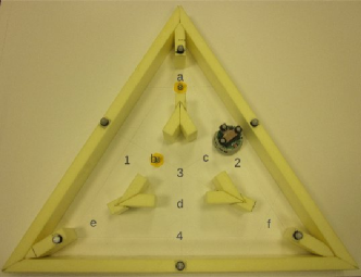
(b) A physical implementation of the game.

Figure 3: The non-cooperative game used in this case study. Figure 3(a) is a graphical depiction of the triangular apartment game, while Fig. 3(b) shows a physical realization of the scenario, with a Khepera II miniature mobile robot in the role of the hybrid agent. The robot localizes itself and observes which doors are closed (door closure implemented manually using the yellow caution cones) through a vicon™ motion capture system. The grammatical inference module and the strategy computation algorithm have been implemented in python, which communicates with the control for the robot (through Matlab™) over a serial link.

The Khepera II, manufactured by K-Team Inc., is a differential-drive mobile robot, with two actuated wheels and kinematics that are accurately represented by the equations of a unicycle. Motion control is achieved through pid loops that independently control either angular displacement or speed of the two wheels. These pid loops can support the development of mid-level motion planning controllers. For example, input-output feedback linearization of the unicycle dynamics [44] leads to a fully actuated reduced system of the form $\dot{q}=u$, where the sequential composition flow-through approach of [45] can be applied to produce controllers that steer the robot from room $i$ to a neighboring room $j$. This same approach has been used in [46] to generate discrete abstractions for the purpose of finding Waldo; details on how the sequential composition approach can give rise to finite state automata abstractions are found in [47].

For the case at hand, we can use the flow-through strategies to generate potential field-based velocity controllers to realize transitions from room $i$ to room $j$ in a way compatible to the requirements on the continuous dynamics of the hybrid agent of Definition 3, that is, ensure that $\text{{Pre}}(\sigma)$ is positively invariant for $f_{\sigma}$, and that trajectories converge to $L^{+}(p,\sigma)\oplus\mathcal{B}_{\varepsilon}$ in finite time (see [47]). The latter set is in fact the formula for $\text{{Post}}(\sigma)$: $x\in L^{+}(p,\sigma)\oplus\mathcal{B}_{\varepsilon}$.

In the context of the flow-through navigation strategy of [45], a transition from, say, room 1 to room 2 (see Fig. 3) would involve a flow-through vector field [45] by which the robot exits the polygon outlining room 1 from the edge corresponding to door $a$ (slightly more sophisticated behavior can be produced by concatenating the flow-through policy with a convergent [45] one that “centers” the robot in room 2.)

The hybrid agent that is obtained by equipping the robot with these flow-through policies can be defined as a tuple $H_{a}=\langle{\mathcal{Z},\Sigma_{a},\iota,\mathcal{P},\pi_{i},\mathcal{AP},f_{\sigma},\text{{Pre}},\text{{Post}},s,T_{a}}\rangle$ where

• $\mathcal{Z}$ is the triangular sector of $\mathbb{R}^{2}$ consisted of the union of the areas of the four rooms.

• $\Sigma_{a}=\{(1,2),\,(1,3),\,(1,4),\,(2,1),\,(2,3),\,(2,4),\,(3,1),\,(3,2),\,(3,4),\,(4,1),\,(4,2),\,(4,3)\}$, with each element associated with a single flow-through policy: $(i,j)$ denotes a flow-through policy from room $i$ to room $j$.

• $\iota:\Sigma_{a}\to\{1,\,2,\,3,\,4\}$ where we slightly abuse notation and define $\iota$ not as a bijection but rather a surjection, where we abstract away the room of origin and we maintain the destination, for simplicity.

• $\pi_{i}=\pi=I$ (the identity), $\mathcal{P}=\mathcal{Z}$, and $s(z,p)=\mathcal{P}$, $\forall(z,p)\in\mathcal{Z}\times\mathcal{P}$; in this case we do not have to use parameters explicitly—they are hard-wired in the flow-through policies.

• $\mathcal{AP}=$ $\{\alpha_{i}:\text{ robot in room }i\}$, $i=1,2,3,4$.

• $f_{\sigma}=K(X_{\sigma}-\dot{q})$, $K>0$, a simple proportional controller on velocity intended to align the system’s vector field with the flow-through field $X_{\sigma}$.

• $\text{{Pre}}\big{(}(i,\cdot)\big{)}=\alpha_{i}$, $i\in\{1,\ldots,4\}$ and $\text{{Post}}\big{(}(\cdot,j)\big{)}=\alpha_{j}$, $j\in\{1,\ldots,4\}$.

• $T_{a}$ following Definition 3, once all other components are defined.

One can verify by inspection when constructing $A(H_{a})$, that the first element of $\sigma=(i,j)$ is encoded in the label for the discrete state, $\alpha_{i}$, from which the transition $\alpha_{i}\stackrel{{\scriptstyle(i,j)}}{{\to}}\alpha_{j}$. Thus, to simplify notation, we change the label of a state from $\alpha_{i}$ to $i$, and the label of the transition from $(i,j)$ to just $j$—the destination state. We write $i\stackrel{{\scriptstyle j}}{{\to}}j$ instead. Figure 4 (left) gives a graphical representation of $A(H_{a})$ after the state/transition relabeling, basically expressing the fact that with all doors open, the robot can move from any room to any other room by initiating the appropriate flow-through policy.

VI-B Results

Suppose the adversarial environment adheres to the Opposite rule in Table I. The SA $A_{1}$ for the agent (player 1) and a fragment of SA $A_{2}$ modeling the environment (player 2) are shown in Fig. 4. By assigning $I_{1}=Q_{1}$ and $I_{2}=Q_{2}$, the game can start with any state in $Q_{1}\times Q_{2}\times\{\bm{1}\}$.

Figure 4: Semiautomata for the agent (left) and for a fragment of the environment (right). In $A_{1}$, the states are the rooms and the transitions are labeled with the rooms that the agent is to enter. For $A_{2}$, the states represent the pairs of doors that are currently closed and a transition $xy$ indicates the pair of doors $x,y$ are to be closed.

The goal of the agent in this example is to visit all four rooms (in any order). Therefore, the specification can be described by the union of shuffle ideals of the permutations of $1234$. In this special case, since the robot occupies one room when game starts, $\mathcal{A}_{s}=\langle Q_{s},\Sigma_{s}=\Sigma_{1}\cup\Sigma_{2},T_{s},I_{s}=\{1,2,3,4\},F_{s}=\{1234\}\rangle$. A fragment of $\mathcal{A}_{s}$ is shown in Fig. 5.

Figure 5: Fragment of $\mathcal{A}_{s}=\langle Q_{s},\Sigma_{s}=\Sigma_{1}\cup\Sigma_{2},T_{s},I_{s}=\{1,2,3,4\},F_{s}=\{1234\}\rangle$, where $x=\Sigma_{2}$.

The interaction functions follow from obvious physical constraints: when the environment adversary closes a door, the agent cannot then move through it. The interaction function $U_{2}(d_{1}d_{2},r)$ gives the set of rooms the agent cannot access from room $r$ because doors $d_{1}$ and $d_{2}$ are closed. In Fig. 3(b), for instance, $U_{2}(ab,1)=\{2,3\}$. In this example, the agent cannot enforce any constraints on the adversary’s behavior, so $U_{1}(q)=\emptyset,\forall q\in Q_{1}\times Q_{2}$. Figure 6 shows a fragment of $A_{1}\circ A_{2}$, while a fragment of the game automaton $\mathcal{G}$ is shown in Fig. 7.

Figure 6: Fragment of turn-based product $P=A_{1}\circ A_{2}=\langle Q_{p},\Sigma_{1}\cup\Sigma_{2},T_{p}\rangle$. State $(r,d_{1}d_{2},c)$ means the agent is in room $r$, doors $\{d_{1},d_{2}\}$ are closed and the Boolean variable keeping track of whose turn it is set to $c$.

Figure 7: Fragment of the game automaton $\mathcal{G}=\langle Q,\Sigma_{1}\cup\Sigma_{2},T,Q_{0},F\rangle$ for the door-robot game, where $Q_{0}=\left\{(q_{1},q_{2},\bm{1},q_{s})\mid q_{1}\in I_{1},q_{2}\in I_{2},q_{s}=q_{1}\in\{1,2,3,4\}\right\}$ and $F=\left\{(q_{1},q_{2},\bm{0},1234)\mid(q_{1},q_{2},\bm{0})\in Q_{p}\right\}$, note that upon initialization of a game, the state of $A_{1}$ (the room occupied by the robot) determines the choice of initial state in $\mathcal{A}_{s}$ (the room visited by the robot.)

Let us show how Proposition 2 applies to this case study. The winning set of states is $F=\{\big{(}(q_{1},q_{2},\bm{0}),1234\big{)}\in Q\mid(q_{1},q_{2},\bm{0})\in Q_{p}\}$; $\mathsf{Attr}(F)$ is obtained by computing the fixed-point of (2). Due to space limitations, we only give a winning path for the robot according to the winning strategy $\mathsf{WS}^{*}_{1}$ with the initial setting of the game in $Q_{0}$.

If the agent were to have complete knowledge of the game automaton, it could compute the set of initial states from which it has a winning strategy:

$$Q_{0}\cap\mathsf{Attr}(F)=\big{\{}(1,ad,\bm{1},1),(1,ce,\bm{1},1),(2,ad,\bm{1},2),(2,bf,\bm{1},2),(4,ce,\bm{1},4),(4,bf,\bm{1},4)\big{\}}.$$

Hence, with complete game information, the robot can win the game starting from initial conditions in $Q_{0}\cap\mathsf{Attr}(F)$; note that $\frac{|Q_{0}\cap\mathsf{Attr}(F)|}{|Q_{0}|}$ makes up a mere $25\%$ of all possible initial configurations. For instance, the agent has no winning strategy if it starts in room $3$.

For the sake of argument, take $q_{0}=(1,ad,\bm{1},1)\in\mathsf{Attr}(F)\cap Q_{0}$. Since the rank of $q_{0}$ is $\rho(q_{0})=7$, following $\mathsf{WS}^{*}_{1}$ of (3) the robot’s fastest winning play is

$$(1,ad,\bm{1},1)\stackrel{{\scriptstyle 4}}{{\rightarrow}}(4,ad,\bm{0},14)\stackrel{{\scriptstyle ae}}{{\rightarrow}}(4,ae,\bm{1},14)\stackrel{{\scriptstyle 2}}{{\rightarrow}}(2,ae,\bm{0},124)\stackrel{{\scriptstyle ce}}{{\rightarrow}}\\ (2,ce,\bm{1},124)\stackrel{{\scriptstyle 1}}{{\rightarrow}}(1,ce,\bm{0},124)\stackrel{{\scriptstyle ef}}{{\rightarrow}}(1,ef,\bm{1},124)\stackrel{{\scriptstyle 3}}{{\rightarrow}}(3,ef,\bm{0},1234)\enspace.$$

The adversary’s moves, $ae$, $ce$ and $ef$, are selected such that it can slow down the process of winning of the robot as much as possible; there is no move the environment can make to prevent the agent from winning since the initial state is in the agent’s attractor and the agent has full knowledge of the game. Note that in the cases where the game rules are described by Adjacent and General regimes (see Table I), the robot cannot win no matter which initial state is in because in both cases $\mathsf{Attr}(F)\cap Q_{0}=\emptyset$. In these game automata, the agent, even with perfect knowledge of the behavior of the environment, can never win.

Let us show how a robot, which has no prior knowledge of the game rules but is equipped with a GIM, can start winning the game after a point when it has observed enough to construct a correct model of its environment. As the first game starts, the agent realizes that the environment is not static, but is rather expressed by some (discrete) dynamical system, a SA $A_{2}$. It assumes (rightfully so in this case) that the language admissible in $A_{2}$ is strictly 2-local. With these knowledge, the robot’s initial hypothesis of the environment $A_{2}^{(0)}=\left(\langle Q_{2},\Sigma_{2},T_{2}\rangle,\mbox{sw}^{(0)}\right)$ is formulated in two steps: (i) obtain the $\text{\acs{sl}}_{2}$-FSA for $\left\{\Sigma_{2}\setminus\{\epsilon\}\right\}^{\ast}$ and assign $\mbox{sw}^{(0)}(q,\sigma)=1,\forall\sigma\in\Sigma_{2}\setminus\{\epsilon\}$; (ii) add self-loops $T_{2}(q,\epsilon)=q$ and let $\mathrm{sw}^{(0)}(q,\epsilon)=1$ , $\forall q\in Q_{2}$.

In every round, the agent does the best it can: it takes the action suggested by the strategy $\mathsf{WS}_{1}^{\ast}$ constructed based on its its current theory of mind. Each time it observes a new action on the part of its adversary, it updates its theory of mind using (4), recomputes $\mathsf{WS}_{1}^{\ast}$ using (3), and applies the new strategy in the following round. The agent may realize that it has lost the game if it finds its current state out of the attractor computed based on its most recent theory of mind. In this case, the agent resigns and starts a new game from a random initial condition, keeping the model for the environment it has built so far and improving it as it goes. We set an upper limit to the number of games by restricting the total number of turns played to be less than $n$.

The following simplified algorithm illustrates the procedure.

1. Let $i=0$, the game hypothesis is $\mathcal{G}^{(0)}$. The game starts with a random $q_{0}\in Q_{0}$.

2. At the current state $q=(q_{1},q_{2},\bm{1},q_{s})$, if the number of turns exceeds the upper limit $n$, the sequence of repeated games is terminated. Otherwise, the robot computes $\mathsf{Attr}(F)$ based on $\mathcal{G}^{(i)}$ (note that it is not necessary to compute $\mathsf{Attr}(F)$ and $\mathsf{WS}_{1}^{\ast}(q)$ as long as there is no update in $\mathcal{G}^{(i)}$ from the previous round.) Then, according to $\mathsf{Attr}(F)$ and (6), the robot either makes a move $\sigma\in\mathsf{WS}_{1}^{\ast}(q)$ or resigns. If a move is made and $T(q,\sigma)\in F$, the robot wins. In the case of either winning or resigning the game, the robot restarts the game at some $q_{0}\in Q_{0}$ with a theory of mind $A_{2}^{(i)}$ and a hypothesized game automaton $\mathcal{G}^{(i)}$; then its control goes to Step 2. Otherwise, it goes to Step 3.

3. The adversary takes some action. The robot observes this action and determines whether to switch on a blocked transition. If a new transition in $A_{2}^{(i)}$ is observed, it updates $A_{2}^{(i)}$ to $A_{2}^{(i+1)}$. Then $\mathcal{G}^{(i)}$ is updated to $\mathcal{G}^{(i+1)}$ according to (5). Otherwise, $A_{2}^{(i+1)}=A_{2}^{(i)}$ and $\mathcal{G}^{(i+1)}=\mathcal{G}^{(i)}$. The robot sets $i=i+1$ and goes to Step 2.

We can measure the efficiency of the learning algorithm by computing the ratio between transitions that are switched on during the game sequence versus the total number of enabled transitions in the true game automaton. The convergence of learning is shown in Fig. 8(a) and the results show that after 125 turns including both robot’s and environment’s turns (approximately 42 games), the robot’s model of the environment converges to the actual one.

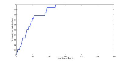
(a) The convergence of learning algorithm. The figure shows the ratio of adversary transitions that have been identified by the agent versus the number of turns the two players have played. In just 125 turns the hybrid agent has full knowledge of its adversary’s dynamics.

	Num of games	Num of wins
No learning	300	0
With learning	300	79
Full knowledge	300	82

(b) Comparison results with three types of the robot. For the case of “no learning,” the robot eventually moves out of its attractor and gets trapped.

Table 8(b) gives outcomes of repeated games in three different scenarios for the robot: (a) Full-Knowledge: the robot knows exactly the model of the environment; (b) No Learning: the robot has no knowledge of, and no way of identifying the environment dynamics, and (c) Learning: the robot starts without prior knowledge of environment dynamics but utilizes a GIM. The initial conditions for the game are chosen randomly. In the absence of prior information about the environment dynamics, and without any process for identifying it, the robot cannot win: in 300 games, it scores no victories. If it had full knowledge of this dynamics, it would have been able to win 82 out of the 300 times it played the game, a percentage of $27\%$, which is close to the theoretical value of $25\%$. A robot starting with no prior knowledge but uses its GIM performs just as well (reaching a win ratio of $26\%$) as one with full knowledge. In fact, as Fig. 8(a) suggests, the robot has recovered the performance of an “all-knowing” agent in less than 15% ($\frac{42}{300}$) of the number of games played repetitively used in Table 8(b). We demonstrate the planning and control of the robot using KiKS simulation environment in Matlab™.

VII Discussion and Conclusions

This paper shows how the use of grammatical inference in robotic planning and control allows an agent to perform a task in an unknown and adversarial environment. Within a game-theoretic framework, it is shown that an agent can start from an incomplete model of its environment and iteratively update that model via a string extension learner applied to the language of its adversary’s turns in the game, to ultimately converge on the correct model. Its success is guaranteed provided that the language being learned is in the class of languages that can be inferred from a positive presentation and the characteristic sample can be observed. This method leads to more effective planning, since the agent will win the game if it is possible for it to do so. Our primary contribution is thus a demonstration of how grammatical inference and game theory can be incorporated in symbolic planning and control of a class of hybrid systems with convergent closed loop continuous dynamics.

The architecture (framework) we propose is universal and can be seen as being composed of two distinct blocks: Control synthesis and Learning. The contents of these blocks can vary according to the task in consideration and the target model to be learned. The current task is a reachability problem, and hence we utilize algorithms for computing a winning strategy in reachability games to synthesize symbolic controllers. However, there is nothing inherent in the architecture that prevents synthesis of the control using winning strategies of other types of games, such as Büchi games[48, 49]. Similarly, as in this paper the rules of the environment are encoded in strictly $k$-local grammar, the learning module operates on string extension languages. However, any language that is identifiable from positive presentation can be considered. The main difference compared to our learning module and other machine learning methods—such as reinforcement learning and Bayesian inference—is that we take advantage of prior knowledge about the structure of the hypothesis space. This assumption enables the development of faster and more efficient learning algorithms.

References

- [1] H. Tanner, J. Fu, C. Rawal, J. Piovesan, and C. Abdallah, “Finite abstractions for hybrid systems with stable continuous dynamics,” Discrete Event Dynamic Systems, vol. 22, pp. 83–99, 2012.
- [2] G. E. Fainekos, A. Girard, H. Kress-Gazit, and G. J. Pappas, “Temporal logic motion planning for dynamic robots,” Automatica, vol. 45, no. 2, pp. 343–352, Feb. 2009.
- [3] C. de la Higuera, Grammatical Inference: Learning Automata and Grammars. Cambridge University Press, 2010.
- [4] W. Zielonka, “Infinite games on finitely coloured graphs with applications to automata on infinite trees,” Theoretical Computer Science, vol. 200, no. 1–2, pp. 135–183, 1998.
- [5] P. J. Ramadge and W. M. Wonham, “Supervisory Control of a Class of Discrete Event Processes,” SIAM Journal on Control and Optimization, vol. 25, no. 1, pp. 206–230, 1987.
- [6] J. Knight and B. Luense, “Control theory, modal logic, and games,” in Hybrid Systems: Computation and Control, ser. Lecture Notes in Computer Science, P. Antsaklis, W. Kohn, A. Nerode, and S. Sastry, Eds. Springer Berlin / Heidelberg, 1997, vol. 1273, pp. 160–173.
- [7] E. Grädel, W. Thomas, and T. Wilke, Eds., Automata logics, and infinite games: a guide to current research. New York, NY, USA: Springer-Verlag New York, Inc., 2002.
- [8] N. Piterman and A. Pnueli, “Synthesis of reactive(1) designs,” in In Proceedings of Verification, Model Checking, and Abstract Interpretation. Springer, 2006, pp. 364–380.
- [9] C. Belta, A. Bicchi, M. Egerstedt, E. Frazzoli, E. Klavins, and G. Pappas, “Symbolic planning and control of robot motion,” IEEE Robotics Automation Magazine, vol. 14, no. 1, pp. 61–70, 2007.
- [10] M. Lahijanian, J. Wasniewski, S. Andersson, and C. Belta, “Motion planning and control from temporal logic specifications with probabilistic satisfaction guarantees,” in IEEE International Conference on Robotics and Automation, 2010, pp. 3227–3232.
- [11] A. LaViers, M. Egerstedt, Y. Chen, and C. Belta, “Automatic generation of balletic motions,” in Proceedings of the 2011 IEEE/ACM Second International Conference on Cyber-Physical Systems, Washington, DC, USA, 2011, pp. 13–21.
- [12] T. Wongpiromsarn, U. Topcu, and R. M. Murray, “Receding horizon control for temporal logic specifications,” in Hybrid Systems: Computation and Control, K. H. Johansson and W. Yi, Eds. New York, NY, USA: ACM, 2010, pp. 101–110.
- [13] C. J. Tomlin, I. Mitchell, A. M. Bayen, and M. Oishi, “Computational techniques for the verification of hybrid systems,” Proceedings of the IEEE, vol. 91, no. 7, pp. 986–1001, july 2003.
- [14] M. Kloetzer and C. Belta, “Dealing with nondeterminism in symbolic control,” in Hybrid Systems: Computation and Control, ser. Lecture Notes in Computer Science, M. Egerstedt and B. Mishra, Eds. Springer, 2008, pp. 287–300.
- [15] H. Kress-Gazit, G. E. Fainekos, and G. J. Pappas, “Temporal-logic-based reactive mission and motion planning,” IEEE Transactions on Robotics, vol. 25, no. 6, pp. 1370–1381, dec. 2009.
- [16] H. Kress-Gazit, T. Wongpiromsarn, and U. Topcu, “Correct, reactive, high-level robot control,” Robotics Automation Magazine, IEEE, vol. 18, no. 3, pp. 65 –74, sept. 2011.
- [17] K. J. Astrom and B. Wittenmark, Adaptive Control. Addison-Wesley, 1995.
- [18] S. Sastry and M. Bodson, Adaptive Control. Prentice Hall, 1989.
- [19] M. J. Matarić, “Reinforcement learning in the multi-robot domain,” Autonomous Robots, vol. 4, no. 1, pp. 73–83, 1997.
- [20] J. Peters, S. Vijayakumar, and S. Schaal, “Reinforcement learning for humanoid robotics,” in Proceedings of the IEEE-RAS International Conference on Humanoid Robots, 2003.
- [21] E. Brunskill, B. R. Leffler, L. Li, M. L. Littman, and N. Roy, “Provably efficient learning with typed parametric models,” Journal of Machine Learning Research, vol. 10, pp. 1955–1988, 2009.
- [22] P. Abbeel, A. Coates, and A. Y. Ng, “Autonomous helicopter aerobatics through apprenticeship learning,” International Journal of Robotics Research, vol. 29, no. 13, pp. 1608–1639, 2010.
- [23] A. Hamdi-Cherif and C. Kara-Mohammed, “Grammatical inference methodology for control systems,” WSEAS Transaction on Computers, vol. 8, no. 4, pp. 610–619, Apr. 2009.
- [24] C. B. Yushan Chen, Jana Tumova, “LTL robot motion control based on automata learning of environmental dynamics,” in IEEE International Conference on Robotics and Automation, Saint Paul, MN, USA, 2012.
- [25] E. M. Gold, “Language identification in the limit,” Information and Control, vol. 10, no. 5, pp. 447–474, 1967.
- [26] J. Heinz, “String extension learning,” in Proceedings of the 48th Annual Meeting of the Association for Computational Linguistics, Uppsala, Sweden, July 2010, pp. 897–906.
- [27] A. Kasprzik and T. Kötzing, “String extension learning using lattices,” in Language and Automata Theory and Applications: 4th International Conference, LATA 2010, ser. Lecture Notes in Computer Science, C. Martin-Vide, H. Fernau, and A. H. Dediu, Eds., vol. 6031. Trier, Germany: Springer, 2010, pp. 380–391.
- [28] R. McNaughton and S. Papert, Counter-Free Automata. MIT Press, 1971.
- [29] A. De Luca and A. Restivo, “A characterization of strictly locally testable languages and its application to subsemigroups of a free semigroup,” Information and Control, vol. 44, no. 3, pp. 300–319, Mar. 1980.
- [30] P. Garcia, E. Vidal, and J. Oncina, “Learning locally testable languages in the strict sense,” in Proceedings of the Workshop on Algorithmic Learning Theory, 1990, pp. 325–338.
- [31] J. Rogers, “Cognitive complexity in the sub-regular realm,” UCLA Colloquium, Oct. 2010.
- [32] J. Lygeros, K. Johansson, S. Simić, and S. Sastry, “Dynamical properties of hybrid automata,” IEEE Transactions on Automatic Control, vol. 48, no. 1, pp. 2–17, 2003.
- [33] H. Enderton, A Mathematical Introduction to Logic. Academic Press, 1972.
- [34] H. Khalil, Nonlinear Systems, 3rd ed. Prentice Hall, 2002.
- [35] C. Stirling, “Modal and temporal logics for processes,” in Logics for concurency: structure vs automata, F. Moller and G. Birtwistle, Eds. Springer, 1996.
- [36] E. M. Clarke Jr., O. Grumberg, and D. A. Peled, Model checking. MIT Press, 1999.
- [37] D. Perrin and J. Éric Pin, Infinite words:automata, semigroups, logic and games. Elsevier, 2004.
- [38] W. Thomas, “Infinite games and verification (extended abstract of a tutorial),” in Proceedings of the 14th International Conference on Computer Aided Verification, ser. CAV ’02. London, UK, UK: Springer-Verlag, 2002, pp. 58–64.
- [39] U. Frith and C. Frith, “Development and neurophysiology of mentalizing,” Philosophical Transactions of the Royal Society B Biological Sciences, no. 358, pp. 459–473, 2003.
- [40] D. Premack and G. Woodruff, “Does the chimpanzee have a theory of mind?” Behavioral and Brain Sciences, vol. 1, no. 04, pp. 515–526, 1978.
- [41] P. Caron, “LANGAGE: a maple package for automaton characterization of regular languages,” in Automata Implementation, ser. Lecture Notes in Computer Science, D. Wood and S. Yu, Eds. Springer, 1998, vol. 1436, pp. 46–55.
- [42] J. Heinz, “Inductive learning of phonotactic patterns,” Ph.D. dissertation, University of California, Los Angeles, 2007.
- [43] J. Fu and H. G. Tanner, “Optimal planning on register automata,” in American Control Conference, Jun 2012 (to appear).
- [44] A. K. Das, R. Fierro, V. Kumar, B. Southall, J. Spletzer, and C. J. Taylor, “Real-time vision-based control of a nonholonomic mobile robot,” in Proceedings of the IEEE International Conference on Robotics and Automation, 2001, pp. 1714–1719.
- [45] D. C. Conner, H. Choset, and A. A. Rizzi, “Flow-through policies for hybrid controller synthesis applied to fully actuated systems,” IEEE Transactions on Robotics, vol. 25, no. 1, pp. 136–146, 2009.
- [46] H. Kress-Gazit, G. E. Fainekos, and G. J. Pappas, “Where’s Waldo? sensor-based temporal logic motion planning,” in Proceedings of the IEEE International Conference on Robotics and Automation, 2007, pp. 3116–3121.
- [47] D. C. Conner, “Integrating planning and control for constrained dynamical systems,” Ph.D. dissertation, Carnegie Mellon University, December 2007.
- [48] R. Mazala, “Infinite games,” in Automata, Logics, and Infinite Games, 2001, pp. 23–42.
- [49] K. Chatterjee, T. Henzinger, and N. Piterman, “Algorithms for Büchi games,” in Games in Design and Verification, 2006.