Studying Superfluid Transition of a Dilute Bose Gas
by Conserving Approximations

Abstract

We consider the Bose-Einstein transition of homogeneous weakly interacting spin-0 particles based on the normal-state $\Phi$-derivable approximation. Self-consistent calculations of Green’s function and the chemical potential with several approximate $\Phi$’s are performed numerically as a function of temperature near $T_{\rm c}$, which exhibit qualitatively different results. The ladder approximation apparently shows a continuous transition with the prefactor $c=2.94$ for the transition-temperature shift $\Delta T_{\rm c}/T_{\rm c}^{0}=can^{1/3}$ given in terms of the scattering length $a$ and density $n$. In contrast, the second-order, particle-hole, and fluctuation-exchange approximations yield a first-order transition. The fact that some standard $\Phi$’s predict a first-order transition challenges us to clarify whether or not the transition is really continuous.

I Introduction

The Bose-Einstein condensation (BEC) of homogeneous weakly interacting Bose gases has attracted much attention over a decade.GCL97 ; HGL99 ; Baym99 ; Baym99-2 ; Holzmann99 ; Baym00 ; Arnold00 ; AM01 ; KPS01 ; CPRS02 ; Kleinert03 ; Kastening03 ; Andersen04 ; LHK04 ; NL04 ; BGW06 ; PGP08 As shown by Baym et al.,Baym99 ; Baym99-2 this topic is profound enough to require treatments beyond the simple perturbation expansion. To be specific, they confirmed that the transition temperature $T_{\rm c}$ starts to increase linearly with the $s$-wave scattering length $a$ as

$$\Delta T_{\rm c}/T_{\rm c}^{0}=can^{1/3},$$ (1)

where $n$ is the density, and presented analytic estimates for the prefactor $c$ using various approximations for Green’s function. Subsequently, a couple of Monte Carlo simulations on finite lattices obtained a widely accepted value $c\approx 1.3$.AM01 ; KPS01

However, these studies as well as othersGCL97 ; HGL99 ; Baym99 ; Baym99-2 ; Holzmann99 ; Baym00 ; Arnold00 ; AM01 ; KPS01 ; CPRS02 ; Kleinert03 ; Kastening03 ; Andersen04 ; LHK04 ; NL04 ; BGW06 ; PGP08 focused mostly on the critical density by implicitly assuming a continuous transition, thereby leaving behind an important question of how the system approaches the critical point as a function of temperature.

We will consider the issue based on the conserving $\Phi$-derivable approximation.LW60 ; Baym62 ; BS89 ; Kita10b This systematic approximation scheme has several remarkable advantages,Kita10b as may be realized by the fact that the Bardeen-Cooper-Scheriffer theory of superconductivity belongs to it as a lowest-order approximation,Kita11b and has been used extensively to clarify anomalous properties of high-$T_{\rm c}$ cuprate superconductors.BS89 Thus, the method will help us to see the critical region of BEC more closely. Indeed, the contents here may be regarded as an extension of those with self-consistent approximations by Baym et al.  Baym99 ; Baym99-2 just on $T=T_{\rm c}$ to (i) incorporate temperature dependences of $T\gtrsim T_{\rm c}$ and (ii) consider more approximations systematically. We will thereby find that the self-consistent one bubble approximation they considered yields a first-order transition contrary to their assumption. The main results are summarized in §3.2 below.

II Formulation

II.1 Hamiltonian and Green’s function

We will consider identical homogeneous bosons with spin $0$, mass $m$, and density $n$ interacting via a weak contact potential $U\delta({\bf r}_{1}-{\bf r}_{2})$. To study this system near $T_{\rm c}$, we adopt the units

$$m=\frac{1}{2},\hskip 14.22636ptn=\frac{\zeta(3/2)}{(4\pi)^{3/2}},\hskip 14.22636ptk_{\rm B}=\hbar=1,$$ (2)

where $\zeta(3/2)\!=\!2.612\cdots$ is the Riemann zeta function and $k_{\rm B}$ denotes the Boltzmann constant. Thus, the critical temperature of the ideal Bose gas,AL03 ; PS08 $T_{\rm c}^{0}=(2\pi\hbar^{2}/k_{\rm B}m)[n/\zeta(3/2)]^{2/3}$, is set equal to $1$, and the kinetic energy is expressed in terms of the momentum ${\bm{p}}$ simply as $\epsilon_{\bm{p}}=p^{2}$.

The Hamiltonian is given by

$$H=\sum_{\bm{p}}(\epsilon_{\bm{p}}-\mu)c_{\bm{p}}^{\dagger}c_{\bm{p}}+\frac{U}{2}\sum_{{\bm{p}}_{1}{\bm{p}}_{2}{\bm{q}}}c_{{\bm{p}}_{1}+{\bm{q}}}^{\dagger}c_{{\bm{p}}_{2}-{\bm{q}}}^{\dagger}c_{{\bm{p}}_{2}}c_{{\bm{p}}_{1}},$$ (3)

where $\mu$ is the chemical potential and $c_{\bm{p}}^{\dagger}$ and $c_{\bm{p}}$ are the creation and annihilation operators, respectively. Ultraviolet divergences inherent in the continuum model are cured here by introducing a momentum cutoff $p_{\rm c}\gg 1$. However, our final results will be free from $p_{\rm c}$, as seen below. It is standard in the low-density limit to remove $U$ in favor of the $s$-wave scattering length $a$. They are connected in the conventional units byPS08

$$\frac{m}{4\pi\hbar^{2}a}=\frac{1}{U}+\int\frac{{\rm d}^{3}p}{(2\pi\hbar)^{3}}\frac{\theta(p_{\rm c}-p)}{2\epsilon_{\bm{p}}}$$

with $\theta(x)$ the step function, which in the present units reads $1/8\pi a=1/U+p_{\rm c}/4\pi^{2}$. We will focus on the limit $a\rightarrow 0$ and choose $p_{\rm c}$ so that $1\ll p_{\rm c}\ll\pi/2a$ is satisfied. Thus, we can set

$$U=8\pi a$$ (4)

to an excellent approximation.

Let us introduce Green’s function in the normal state by

$$G(\vec{p}\,)=\frac{1}{i\varepsilon_{n}-\epsilon_{\bm{p}}-\Sigma(\vec{p}\,)+\mu},$$ (5a)

where $$\vec{p}\equiv({\bm{p}},i\varepsilon_{n}) \varepsilon_{n}\!=\!2n\pi T n\!=\!0,\pm 1,\pm 2,\cdots \Sigma(\vec{p}\,)$$ with () a boson Matsubara frequency. The self-energy is given exactly by

$$\Sigma(\vec{p}\,)=-\frac{1}{T}\frac{\delta\Phi}{\delta G(\vec{p}\,)},$$ (5b)

where the functional $\Phi=\Phi[G]$ is defined as the infinite sum of closed skeleton diagrams in the simple perturbation expansion for the thermodynamic potential with the replacement $G_{0}\rightarrow G$.LW60 ; Baym62 ; Kita10b The chemical potential $\mu$ is connected with the particle density $n$ by

$$n=-\frac{T}{{\cal V}}\sum_{\vec{p}}G(\vec{p}\,)\,{\rm e}^{i\varepsilon_{n}0_{+}},$$ (6)

with ${\cal V}$ the volume and $0_{+}$ an infinitesimal positive constant.

If BEC is realized as a continuous transition, the transition temperature $T_{\rm c}$ will be determined by the condition:

$$\mu=\Sigma(\vec{0}).$$ (7)

This relation, which is derived from the Hugenholtz-Pines relation in the condensed phase Kita09 ; HP59 by setting the off-diagonal self-energy zero, naturally extends the condition $\mu_{0}(1)\!=\!0$ for the transition temperature of the ideal gasPS08 to interacting cases. Indeed, it was used by Baym et al. Baym99 ; Baym99-2 to estimate the critical density $n_{\rm c}$.

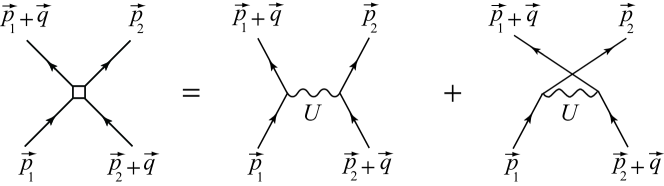
Figure 1: Diagrammatic representation of symmetrized vertex $\Gamma^{(0)}(\vec{p}_{1},\vec{p}_{2},\vec{q})$, which is equal to $2U$ for the contact interaction $U\delta({\bm{r}}_{1}-{\bm{r}}_{2})$ used here.

II.2 FLEX and related approximations

The $\Phi$-derivable approximation consists of (i) retaining some finite terms or partial series in $\Phi[G]$ and calculating $G$ and $\Sigma$ self-consistently by eqs. (5a) and (5b). We will consider the fluctuation-exchange (FLEX) approximationBS89 and those derivable from it by reducing terms. All of them are concisely expressible in terms of the symmetrized vertex $\Gamma^{(0)}(\vec{p}_{1},\vec{p}_{2},\vec{q})$ of Fig. 1, which is equal to $2U$ with no momentum and frequency dependence for the present contact interaction $U\delta({\bm{r}}_{1}-{\bm{r}}_{2})$.AGD63

To begin with, $\Phi_{\rm FLEX}$ is given as a sum of four kinds of diagrams in Fig. 2 as

$$\Phi_{\rm FLEX}=\Phi_{1}+\Phi_{2}+\Phi_{\rm ph}+\Phi_{\rm pp},$$ (8)

where $\Phi_{1}\equiv{\cal V}Un^{2}$ is the Hartree-Fock term. To express the other contributions analytically, let us introduce the functions

$$\chi_{\rm ph}(\vec{q}\,)\equiv\frac{T}{{\cal V}}\sum_{\vec{p}}G(\vec{p}\,)G(\vec{p}+\vec{q}\,),$$ (9a)

$$\chi_{\rm pp}(\vec{q}\,)\equiv\frac{T}{{\cal V}}\sum_{\vec{p}}G(\vec{p}\,)G(-\vec{p}+\vec{q}\,),$$ (9b)

each of which corresponds to a pair of lines connecting adjacent vertices in Fig. 2(c) and (d), respectively. By following the Feynman rules for the perturbation expansion in terms of $\Gamma^{(0)}\!=\!2U$,Kita11b the numerical factor of Fig. 2(b) and those of the $n$th-order diagrams ($n=3,4,\cdots$) in Fig. 2(c) and (d) are easily found as $c_{2}=-(-2U)^{2}2^{2}T/4^{2}2!=-U^{2}T/2$, $c^{(n)}_{\rm ph}=-(-2U)^{n}2^{2n-1}(n-1)!T/4^{n}n!=(-2)^{n-1}U^{n}T/n$, and $c^{(n)}_{\rm pp}=-(-2U)^{n}2^{n}(n-1)!T/4^{n}n!=(-1)^{n-1}U^{n}T/n$. We thereby obtain analytic expressions for Fig. 2(b)-(d) as

$$\Phi_{2}=-\frac{T}{2}\sum_{\vec{q}}[U\chi_{\rm ph}(\vec{q}\,)]^{2}=-\frac{T}{2}\sum_{\vec{q}}[U\chi_{\rm pp}(\vec{q}\,)]^{2},$$ (10a)

$$\Phi_{\rm ph}=\frac{T}{2}\sum_{\vec{q}}\biggl{\{}\ln[1+2U\chi_{\rm ph}(\vec{q}\,)]-2U\chi_{\rm ph}(\vec{q}\,)$$

$$\hskip 1.42262pt+\frac{[2U\chi_{\rm ph}(\vec{q}\,)]^{2}}{2}\biggr{\}},$$ (10b)

$$\Phi_{\rm pp}=T\sum_{\vec{q}}\biggl{\{}\ln[1+U\chi_{\rm pp}(\vec{q}\,)]-U\chi_{\rm pp}(\vec{q}\,)$$

$$\hskip 1.42262pt+\frac{[U\chi_{\rm pp}(\vec{q}\,)]^{2}}{2}\biggr{\}},$$ (10c)

respectively.

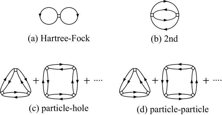
Figure 2: Feynman diagrams for $\Phi_{\rm FLEX}$

Let us substitute eq. (8) into $\Phi$ of eq. (5b). We then obtain the self-energy as

$$\Sigma(\vec{p})=2Un-\frac{T}{{\cal V}}\sum_{\vec{q}}[V_{2}(\vec{q})+V_{\rm ph}(\vec{q})]G(\vec{p}+\vec{q})$$

$$\hskip 5.69054pt-\frac{T}{{\cal V}}\sum_{\vec{q}}V_{\rm pp}(\vec{q})G(-\vec{p}+\vec{q}),$$ (11)

with

$$V_{2}(\vec{q})\equiv-2U^{2}\chi_{\rm ph}(\vec{q}),$$ (12a)

$$V_{\rm ph}(\vec{q})\equiv 2U\frac{[2U\chi_{\rm ph}(\vec{q})]^{2}}{1+2U\chi_{\rm ph}(\vec{q})},$$ (12b)

$$V_{\rm pp}(\vec{q})\equiv 2U\frac{[U\chi_{\rm pp}(\vec{q})]^{2}}{1+U\chi_{\rm pp}(\vec{q})}.$$ (12c)

Equation (5a) with eq. (11) forms a closed nonlinear equation for $G(\vec{p})$ that may be solved numerically to clarify normal-state properties of $T\geq T_{\rm c}$.

Besides eq. (11), we will also consider the following self-energies:

$$\Sigma_{2}(\vec{p})\equiv 2Un-\frac{T}{{\cal V}}\sum_{\vec{q}}V_{2}(\vec{q})G(\vec{p}+\vec{q}),$$ (13a)

$$\Sigma_{\rm ph}(\vec{p})\equiv 2Un-\frac{T}{{\cal V}}\sum_{\vec{q}}[V_{2}(\vec{q})+V_{\rm ph}(\vec{q})]G(\vec{p}+\vec{q}),$$ (13b)

$$\Sigma_{\rm pp}(\vec{p})\equiv 2Un-\frac{T}{{\cal V}}\sum_{\vec{q}}[V_{2}(\vec{q})G(\vec{p}+\vec{q})$$

$$\hskip 14.22636pt+V_{\rm pp}(\vec{q})G(-\vec{p}+\vec{q})],$$ (13c)

which are all derivable from eq. (11) by reducing terms. Using these different approximations, we may check how well the present approach describes the BEC transition.

Equations (13a) and (13c) were used by Baym et al. Baym99 ; Baym99-2 as “self-consistent one bubble approximation” and “self-consistent ladder sum” for estimating $T_{\rm c}$. They also considered the “self-consistent bubble sum” of setting $V_{\rm ph}(\vec{q})\rightarrow\frac{1}{2}V_{\rm ph}(\vec{q})$ in eq. (13b), which amounts to neglecting the exchange processes altogether in the particle-hole series of Fig. 2(c). Since the exchange processes are definitely present, we will consider eq. (13b) instead of the self-consistent bubble sum.

II.3 Dilute gas near $T_{\rm c}$

We now focus on the critical region of the weak-coupling limit $a\rightarrow 0$, i.e., $T\gtrsim 1$. Noting that this system is quantitatively close to the ideal gas, we first express the chemical potential as

$$\mu=\mu_{0}+\Sigma(\vec{0})+\Delta\mu,$$ (14)

where $\mu_{0}$ is the chemical potential of the ideal gas vanishing quadratically for $T\rightarrow 1$ asAL03

$$\mu_{0}(T)=-c_{0}^{2}(T-1)^{2},\hskip 14.22636ptc_{0}\equiv\frac{3\zeta(3/2)}{4\sqrt{\pi}}.$$ (15)

We also adopt the classical-field approximation by Baym et al. Baym99 ; Baym99-2 of retaining only the $\varepsilon_{n}=0$ component in eq. (5a); its validity will be confirmed shortly. We subsequently perform a change of variables, $T\rightarrow\tau$, $p\rightarrow\tilde{p}$, $\Delta\mu\rightarrow\Gamma$, and $\Sigma({\bm{p}},i\varepsilon_{n}=0)\rightarrow\sigma(\tilde{p})$, given explicitly by

$$T=1+\frac{U}{c_{0}}\tau,$$ (16a)

$$p=U\tau\tilde{p},$$ (16b)

$$\mu_{0}(T)+\Delta\mu(T)=-(U\tau)^{2}\Gamma(\tau),$$ (16c)

$$\Sigma({\bm{p}},i\varepsilon_{n}=0)=\Sigma(\vec{0})+(U\tau)^{2}\sigma(\tilde{p}).$$ (16d)

Note that $\Gamma\rightarrow 1$ and $\sigma(p)\rightarrow 0$ for $U\rightarrow 0$ as seen from eqs. (15) and (16). The change of variables also removes the remaining source of the ultraviolet divergence, i.e., $\Sigma(\vec{0})$, completely from the theory. Substituting eq. (14) into eq. (5a) for $\varepsilon_{n}=0$ and using eq. (16), we can write $G({\bm{p}},i\varepsilon_{n}=0)$ as

$$G({\bm{p}},0)=-\frac{g(\tilde{p})}{(U\tau)^{2}},\hskip 14.22636ptg(p)\equiv\frac{1}{p^{2}+\sigma(p)+\Gamma}.$$ (17)

We also adopt the classical-field approximation for eq. (9) and substitute eqs. (16a), (16b), and (17) into it. It then turns out that $\chi_{\rm ph}({\bm{q}},0)=\chi_{\rm pp}({\bm{q}},0)=\chi(\tilde{q})/U\tau$ with

$$\chi(q)\equiv\int\frac{{\rm d}^{3}p}{(2\pi)^{3}}g(p)g(|{\bm{p}}+{\bm{q}}|).$$ (18)

Subsequently using eqs. (11) and (16d) with eqs. (16a), (16b), and (17), we obtain an equation for the reduced self-energy $\sigma(p)$ as

$$\sigma(p)=\int\frac{{\rm d}^{3}q}{(2\pi)^{3}}v(q)[g(|{\bm{p}}+{\bm{q}}|)-g(q)],$$ (19)

with

$$v(q)\equiv\frac{2}{\tau}\left\{-\frac{\chi(q)}{\tau}+\frac{[2\chi(q)/\tau]^{2}}{1+2\chi(q)/\tau}+\frac{[\chi(q)/\tau]^{2}}{1+\chi(q)/\tau}\right\}.$$ (20)

As for eq. (6) for the chemical potential, we subtract its non-interacting correspondent from it, adopt the classical-field approximation, and use eq. (17). It is thereby transformed into an equation for $\Gamma=\Gamma(\tau)$ as

$$\int_{0}^{\infty}\!\left[\frac{1}{p^{2}+\sigma(p)+\Gamma}-\frac{1}{p^{2}+1}\right]p^{2}{\rm d}p=0.$$ (21)

Equations (19) and (21) form closed equations for $\sigma(p)$ and $\Gamma$ for a given $\tau$. Note that the transformation (16) has removed $U$ completely from the self-consistent equations. Besides, they are free from ultraviolet divergences.

The self-energies of eq. (13) can be transformed similarly, which turn out to have the kernels

$$v_{2}(q)\equiv-\frac{2\chi(q)}{\tau^{2}},$$ (22a)

$$v_{\rm ph}(q)\equiv-\frac{2\chi(q)}{\tau^{2}}\,\frac{1-2\chi(q)/\tau}{1+2\chi(q)/\tau},$$ (22b)

$$v_{\rm pp}(q)\equiv-\frac{2\chi(q)}{\tau^{2}}\,\frac{1}{1+\chi(q)/\tau},$$ (22c)

in place of $v(q)$ in eq. (19). Note that $v_{2}(q)$ and $v_{\rm pp}(q)$ are negative, as seen from eq. (18), whereas $v(q)$ and $v_{\rm ph}(q)$ change sign from negative to positive as $\tau$ is decreased towards zero. These distinct behaviors of the kernels from different approximations will lead to contradictory predictions on the BEC transition, as seen below.

Finally, eq. (7) for the continuous transition point is transformed with eqs. (14) and (16c) into

$$\Gamma(\tau_{\rm c})=0.$$ (23)

The corresponding critical temperature is easily obtained by eq. (16a) with $\tau=\tau_{\rm c}$. Using eqs. (2), (4), and (15) as well as $T_{\rm c}^{0}\!=\!1$ in the present units, we confirm that the transition-temperature shift starts linearly in $a$ as eq. (1) with the prefactor

$$c=\frac{(8\pi)^{2}}{3[\zeta(3/2)]^{4/3}}\tau_{\rm c}=58.52\tau_{\rm c}.$$ (24)

A couple of comments are in order before closing the subsection. First, eq. (19) tells us that diagrams from second through infinite orders in $U$ contribute equivalently to $\sigma(p)$. The validity of this statement is clearly not restricted to the FLEX approximation alone; it can be confirmed easily by applying eqs. (16) and (17) for general $n$th order terms in the classical-field approximation. Thus, we need to include infinite diagrams of $\Phi$ to obtain an exact value of $\tau_{\rm c}$ in the self-consistent perturbation approach, which is practically impossible. We may expect, however, that some approximations for $\Phi$ enable us to obtain qualitatively correct results for the BEC transition. Second, $\varepsilon_{n}\neq 0$ components in eq. (5a) are smaller than the $\varepsilon_{n}=0$ one by $(U\tau)^{2}$ in the critical region so that they are negligible, as seen easily by using the transformation of eq. (16). Thus, the classical-field approximation by Baym et al. Baym99 ; Baym99-2 has also been justified by the present consideration.

III Results

III.1 Numerical procedure

We explain how to solve eqs. (19) and (21) numerically to obtain the reduced self-energy $\sigma(p)$ and reduced chemical potential $\Gamma$ as a function of the reduced temperature $\tau$. Let us introduce the non-interacting correspondent of eq. (18) as

$$\chi^{(0)}(q)\equiv\int\frac{{\rm d}^{3}p}{(2\pi)^{3}}\frac{1}{(|{\bm{p}}+{\bm{q}}/2|^{2}+1)(|{\bm{p}}-{\bm{q}}/2|^{2}+1)}$$

$$\hskip 4.2679pt=\frac{\arctan(q/2)}{4\pi q}.$$ (25)

The second expression has been obtained by (i) performing angular integrations, (ii) subsequently expanding $\ln[(p\pm q/2)^{2}+1]$ in terms of $pq/(p^{2}+q^{2}/4+1)$, (iii) making a change of variables as $p=(q^{2}/4+1)^{1/2}\tan\theta$ and carrying out the $\theta$ integration, and (iv) comparing the resulting series with the Taylor expansion of $\arcsin x$. Noting that $\chi(q)\rightarrow\chi^{(0)}(q)$ for $q\rightarrow\infty$, we realize that $\chi(q)\rightarrow 1/8q$ for $q\gg 1$. Hence, it follows that eq. (19) for $p\gg 1$ is well described by

$$\sigma^{(0)}(p)\equiv\int\frac{{\rm d}^{3}q}{(2\pi)^{3}}\frac{1}{4\tau^{2}q}\left(\frac{1}{q^{2}+1}-\frac{1}{|{\bm{p}}+{\bm{q}}|^{2}+1}\right)$$

$$\hskip 4.2679pt=\frac{\ln(p^{2}+1)-2+(2/p)\arctan p}{(4\pi\tau)^{2}},$$ (26)

where the second expression has been obtained in the same manner as eq. (25).

Equations (19) and (21) have been solved iteratively, starting from the non-interacting Green’s function and chemical potential in the integrands. Functions $\chi(q)$ and $\sigma(p)$ are calculated by using the integral expressions of $\chi(q)-\chi^{(0)}(q)$ and $\sigma(p)-\sigma^{(0)}(p)$ whose integrands decrease more quickly in the high-momentum region than those of eqs. (18) and (19). Further, we make a change of variables $p=\sinh u^{2}$ and $q=\sinh v^{2}$ for the integrations to cover a wide momentum range up to a cutoff momentum $p_{\rm cut}=10^{5}\sim 10^{7}$. We have also stored $\chi(q)$ and $\sigma(p)$ at equal intervals in terms of $v$ and $u$. These values are used in the next step of iteration with interpolation. The region ${\bm{p}}+{\bm{q}}\sim{\bf 0}$ of eqs. (18) and (19) are handled separately to incorporate more integration points in both the polar and radial integrations. The convergence has been checked by changing the number of integration points as well as $p_{\rm cut}$.

The above procedure has been repeated for four different approximations with kernels (20) and (22) to check how reliable the predictions on the BEC transition by the present approach are.

III.2 Results

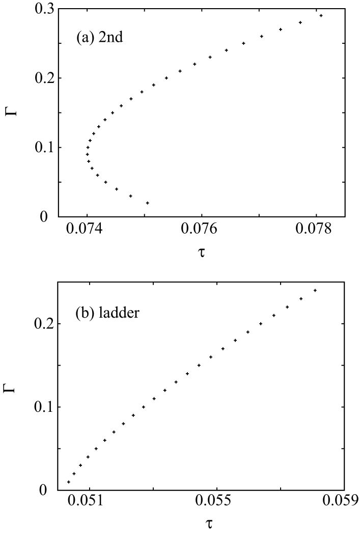
Figure 3: Reduced chemical potential $\Gamma$ as a function of reduced temperature $\tau$ in (a) the self-consistent second-order approximation and (b) self-consistent ladder approximation.

Figure 3 plots reduced chemical potential $\Gamma\propto\Sigma(\vec{0})-\mu$ as a function of reduced temperature $\tau\propto T-1$ in the (a) self-consistent second-order approximation with kernel (22a) and (b) self-consistent ladder approximation with kernel (22c). A continuous BEC transition corresponds to a monotonic decrease of $\Gamma(\tau)$ towards $0$ where BEC is realized. Thus, Fig. 3(b) from the ladder approximation apparently exhibits a continuous BEC transition around $\tau_{\rm c}\!=\!0.0503$, which translates to $\Delta T_{\rm c}/T_{\rm c}^{0}\!=\!2.94an^{1/3}$ by eqs. (1) and (24). On the other hand, Fig. 3(a) from the second-order approximation shows a clear sign of a first-order transition somewhere between $0.074\!\lesssim\!\tau\!\lesssim\!0.076$ where $\Gamma(\tau)$ is multivalued. As for the FLEX approximation, we have not even found a solution that approaches $\Gamma\!=\!0$ continuously; here $\Gamma(\tau)$ has a minimum $\Gamma_{\rm min}\approx 0.95$ around $\tau=0.14$. This strange behavior is brought about by kernel (20) that changes sign from negative to positive as $\tau$ is reduced. The same statement holds for the particle-hole approximation of eq. (22b). Since the present model is quite close to the ideal Bose gas, we may conclude that the BEC transition is a first-order transition in both the FLEX and particle-hole approximations.

With the diversity of predictions in the present approach, we can hardly say anything definite about the nature of the BEC transition with a weak two-body interaction. However, the fact that some standard $\Phi$’s (i.e., $\Phi_{2}$, $\Phi_{\rm 2}+\Phi_{\rm ph}$, and $\Phi_{\rm FLEX}$) exhibit a first-order transition challenges us to clarify unambiguously whether or not the BEC transition is really continuous.

As for the transition temperature shift, the value $\Delta T_{\rm c}/T_{\rm c}^{0}\!=\!2.94an^{1/3}$ in the present ladder approximation departs from the value $\Delta T_{\rm c}/T_{\rm c}^{0}\!\simeq\!2.5an^{1/3}$ obtained by Baym et al.  Baym99-2 with an ultraviolet cutoff $\Lambda$. However, they also reported that their bubble-sum result $\Delta T_{\rm c}/T_{\rm c}^{0}\!\simeq\!1.6an^{1/3}$ for the finite $\Lambda$ is increased up to $2.0an^{1/3}$ by the extrapolation $\Lambda\rightarrow\infty$. Incorporating the same difference $0.4an^{1/3}$ into their ladder-summation result yields $\Delta T_{\rm c}/T_{\rm c}^{0}\!\simeq\!(2.5+0.4)an^{1/3}$, which is in good agreement with $2.94an^{1/3}$ in the present approach. If we use $\tau_{\rm c}\!\simeq\!0.076$ from Fig. 3(a) determined by eq. (23), we obtain $\Delta T_{\rm c}/T_{\rm c}^{0}=4.4an^{1/3}$ for the second-order approximation, which is also in good agreement with $\Delta T_{\rm c}/T_{\rm c}^{0}\!\simeq\!(3.8+0.4)an^{1/3}$ by Baym et al. Baym99-2 However, it should be noted once again that our second-order result clearly indicates a first-order transition contrary to their assumption. In their early study, Baym et al. Baym99 also reported $\Delta T_{\rm c}/T_{\rm c}^{0}\!=\!2.9an^{1/3}$ as eq. (29), which apparently agrees with our ladder result mentioned above. However, their estimate starts from the second-order approximation corresponding to our eq. (13a) and subsequently adopts a trial form $U(k)\approx k^{3/2}k_{\rm c}^{1/2}/[1+(k/k_{\rm c})^{3/2}]$ for $U(k)\equiv 2m[\Sigma_{2}({\bm{k}},i\varepsilon_{n}=0)-\mu]$ at $T=T_{\rm c}$ to interpolate between the low- and high-momentum behaviors of $\epsilon_{\bm{k}}+\Sigma({\bm{k}},i\varepsilon_{n}=0)-\mu$ with an intermediate parameter $k_{\rm c}$. Thus, the agreement is accidental and their prefactor $2.9$ should be replaced by $3.8$($+0.4$) in their later numerical study for the second-order approximation.Baym99-2

- (1) P. Grüter, D. Ceperley and F. Laloë: Phys. Rev. Lett. 79 (1997) 3549.
- (2) M. Holzmann, P. Grüter, and F. Laloë: Eur. Phys. J. B 10 (1999) 739.
- (3) G. Baym, J.-P. Blaizot, M. Holzmann, F. Laloë, and D. Vautherin: Phys. Rev. Lett. 83 (1999) 1703.
- (4) G. Baym, J.-P. Blaizot, M. Holzmann, F. Laloë, and D. Vautherin: Eur. Phys. J. B 24 (2001) 107.
- (5) M. Holzmann and W. Krauth: Phys. Rev. Lett. 83 (1999) 2687.
- (6) G. Baym, J. -P. Blaizot and J. Zinn-Justin: Europhys. Lett. 49 (2000) 150.
- (7) P. Arnold and B. Tomášik: Phys. Rev. A 62 (2000) 063604.
- (8) P. Arnold and G. Moore: Phys. Rev. Lett. 87 (2001) 120401.
- (9) V. A. Kashurnikov, N.V. Prokof fev, and B.V. Svistunov: Phys. Rev. Lett. 87 (2001) 120402.
- (10) F. F. de Souza Cruz, M. B. Pinto, R. O. Ramos, and P. Sena: Phys. Rev. A 65 (2002) 053613.
- (11) H. Kleinert: Mod. Phys. Lett. B 17 (2003) 1011.
- (12) B. Kastening: Phys. Rev. A 68 (2003) 061601(R); Phys. Rev. A 69 (2004) 043613.
- (13) J. O. Andersen: Rev. Mod. Phys. 76 (2004) 599.
- (14) S. Ledowski, N. Hasselmann and P. Kopietz: Phys. Rev. A 69 (2004) 061601(R); N. Hasselmann, S. Ledowski and P. Kopietz: Phys. Rev. A 70 (2004) 063621.
- (15) K. Nho and D. P. Landau: Phys. Rev. A 70 (2004) 053614.
- (16) J.-P. Blaizot, R. Méndez-Galain, and N. Wschebor: Phys. Rev. E 74 (2006) 051116.
- (17) S. Pilati, S. Giorgini, and N. Prokof’ev: Phys. Rev. Lett. 100 (2008) 140405.
- (18) J. M. Luttinger and J. C. Ward: Phys. Rev. 118 (1960) 1417.
- (19) G. Baym: Phys. Rev. 127 (1962) 1391.
- (20) N. E. Bickers and D. J. Scalapino: Ann. Phys. 193 (1989) 206.
- (21) T. Kita: Prog. Theor. Phys. 123 (2010) 581.
- (22) T. Kita: J. Phys. Soc. Jpn. 80 (2011) 124704. See Appendix A for Feynman rules in terms of .
- (23) A. L. Fetter and J. D. Walecka: Quantum Theory of Many-Particle Systems (Dover Publications, Mineola, N.Y., 2003).
- (24) C. J. Pethick and H. Smith: Bose-Einstein Condensation in Dilute Gases (Cambridge University Press, Cambridge, 2008).
- (25) N. M. Hugenholtz and D. Pines: Phys. Rev. 116 (1959) 489.
- (26) T. Kita: Phys. Rev. B 80 (2009) 214502.
- (27) A. A. Abrikosov, L. P. Gorkov, and I. E. Dzyaloshinski: Methods of Quantum Field Theory in Statistical Physics (Prentice-Hall, Englewood Cliffs, N.J., 1963).